Remote Sensing of Environment 144 (2014) 98–108

Contents lists available at ScienceDirect

Remote Sensing of Environment

j ourna l homepage: www.e lsev ie r .com/ locate / rse

Spatial and temporal variability of SST and ocean color in the Gulf ofMaine based on cloud-free SST and chlorophyll reconstructionsin 2003–2012

Yizhen Li ⁎, Ruoying HeDepartment of Marine, Earth, and Atmospheric Sciences, North Carolina State University, Raleigh, NC 27695, United States

⁎ Corresponding author. Tel.: +1 919 513 0943.E-mail address: yli15@ncsu.edu (Y. Li).

0034-4257/$ – see front matter. Published by Elsevier Inchttp://dx.doi.org/10.1016/j.rse.2014.01.019

a b s t r a c t

a r t i c l e i n f o

Article history:Received 23 September 2013Received in revised form 14 January 2014Accepted 19 January 2014Available online xxxx

Keywords:Gulf of MaineChlorophyll bloomSea surface temperatureNorth Atlantic OscillationEOF analysis

The spatial and temporal variability of sea surface temperature (SST) and Chlorophyll-a (Chl-a) in the Gulf ofMaine (GOM) is examined using daily, cloud-free Data INterpolating Empirical Orthogonal Function (DINEOF)reconstructions during 2003–2012. The utility of the DINEOF SST and Chl-a is demonstrated through direct com-parisons with buoy- and ship-based observations. EOF analyses of cloud-free products are further used to quan-tify the SST and Chl-a variability on seasonal to inter-annual timescales. The first mode of SST is dominated by anannual cycle in response to net surface heat flux, with SST lagging surface flux by ~57 days. The second mode ofSST underscores interactions between GOM, the Scotian Shelf, and the slope sea in response to the basin scale at-mospheric forcing represented by the North Atlantic Oscillation. The third mode correlates well with the evolu-tion of Scotian Shelf-slope frontal displacement. The first EOF mode of Chl-a is dominated by a winter–springbloom and a fall bloom, with a spatial distribution modified by the tidal mixing that facilitates nutrient deliveryfrom the deep ocean. The second EOFmode is likely associatedwith awinter bloom in thewarm slope sea, wherethe low-frequency variations of second modes of SST and Chl-a are in phase, suggesting a possible coupling be-tween physical and biological responses to atmospheric forcing. The third mode of the Chl-a is likely associatedwith freshening events associatedwith advection of the Scotian ShelfWater, which enhance stratifications in theeastern GOM.

Published by Elsevier Inc.

1. Introduction

The Gulf of Maine (GOM) is a semi-closed marginal sea off the U.S.northeast coast (Fig. 1). Extensive research in the past on regional circu-lation and hydrography have studied processes on synoptic (e.g.,Churchill, Pettigrew, & Signell, 2005; He et al., 2005), seasonal (e.g.,Lynch, Ip, Naimie, & Werner, 1996; Xue, Chai, & Pettigrew, 2000),and inter-annual time scales (e.g., Li, He, & McGillicuddy, in press;Pettigrew et al., 2005, 1998). The mean gulf circulation is cyclonic(Bigelow, 1927), and modulated by both local and remote forcing. Localforcing includes strong tidal mixing and rectifications (e.g., Garrett,1972; Limeburner & Beardsley, 1996; Lynch, Holboke, & Maimie,1997), surface heat flux (e.g., Xue et al., 2000) and wind (e.g., He &McGillicuddy, 2008). Remote influence stems from surface inflowof relatively cold, fresh Scotian Shelf (SS) water through Cape Sable(Smith, 1983), intrusions of Labrador subarctic Slope Water (LSW)and the Atlantic Warm Slope Water (WSW) through the NortheastChannel (NEC). From time to time, Gulf Stream eddies can also play arole in shaping the slope sea circulation,which in turn affects circulation

.

and transport in the GOM (e.g., Bisagni & Smith, 1998; Chaudhuri,Gangopadhyay, & Bisagni, 2009).

TheGOM is known for high biological productivity. Significant season-al phytoplankton blooms occur every fall and spring, although the exacttimings vary region by region in the gulf due to differences in hydrody-namics, bathymetry, stratification, mixing processes, and nutrient uptake(e.g., O'Reilly & Busch, 1984; O'Reilly, Evans-Zetlin, & Busch, 1987; Yoder,Schollaert, & O'Reilly, 2002; Thomas, Townsend, & Weatherbee, 2003).Research to date on plankton bloom and Chl-a variations have reliedlargely on episodic ship survey data or time series observationsmeasuredby buoys. An inherent practical limitation of this approach is data gapsspatially (Herman et al., 1991; Holligan, Balch, & Yentsch, 1984; O'Reillyet al., 1987; Townsend, Cammen, Holligan,Campbell, & Pettigrew, 1994;Townsend & Thomas, 2001; Townsend & Thomas, 2002). Satellite remotesensing provides a useful means to routinely sample the surface oceanover a larger spatial context. Early studies using remote sensing have ad-dressed the relationship between SST front and shelfbreak bloom (e.g.,Ryan, Yoder, & Cornillon, 1999), ocean environmental variability and itslinkage with shellfish toxicity (e.g., Luerssen, Thomas, & Hurst, 2005;Thomas, Weatherbee, Xue, & Liu, 2010), coastal circulation in easternandwestern GOM (e.g., Pettigrew et al., 2005), andmesoscale eddy activ-ities (e.g., Churchill et al., 2005). Various forms of remote sensing data in-cluding instantaneous snapshots (Yoder, O'Reilly, Barnard, Moore, &

Fig. 1. (a) Spatial distribution of the percent of cloud coverage inMODIS SST during 2003–2012. Major geographic locations and 100- and 200-m isobaths in the Gulf of Maine are shown.Also shown are the locations for NERACOOS buoys A, B, E, F, I, M, and N. Surface temperature data measured by these buoys are used to compare with satellite measured SST. Chl-a con-centrationsmeasured by buoy Station 2 (S2) on the Scotian Shelf are used to comparewith their satellite counterparts. (b) Number of retained daily images used for the reconstruction ofSST in each month during 2003–2012. Only images with less than 98% cloud coverage are retained for the reconstruction.

99Y. Li, R. He / Remote Sensing of Environment 144 (2014) 98–108

Ruhsam, 2001), monthly composite (e.g., Thomas et al., 2003), and long-term climatology (Ji et al., 2007; Yoder et al., 2002) were used/derived tostudy temporal and spatial variation of phytoplankton and Chl-a in theGOM, as well as frontal displacement (Ullman & Cornillon, 1999). Whilesatellites provide more routine and consistent temporal sampling, theirdata can be quite gappy due to cloud cover problem (e.g., Miles & He,2010). As a result, compromises have to be made by computing compos-ite averages over different timeperiods (e.g., weekly ormonthly), limitingthe ability of remote sensing observation in resolving synoptic processes.In addition, previous SST and Chl-a studies for the GOM covered a shortspanof time in the 1990s and early 2000s (Thomas et al., 2003) or focusedon seasonal climatology (Yoder et al., 2002). As such, a study of seasonaland interannual variability based on cloud-free SST and ocean color datafor the GOM based on novel reconstruction techniques in recent decadeis therefore highly needed.

To do this, we used concurrent sea surface temperature (SST) andocean color observations obtained byMODIS (Moderate Resolution Im-aging Spectroradiometer) to investigate simultaneous variations in SSTand surface Chl-a. TheMODIS sensor was launched inMay, 2002 aboardthe synchronous polar orbiting satellite Aqua, thus can provide usefulinformation for surface thermal and productivity structures during thepast decade.MODIS is only capable of viewing in the visible and infrared

wave bands, thus almost all images have cloud cover to various extents.Taking GOM for instance, we see that the average percent of cloud cov-erage is over 60% of the total spatial coverage,with over 80% cloud coverover the Georges Bank and Scotian Shelf (Fig. 1a). To overcome t cloud-cover problem in the satellite data, we utilized a new daily, high-resolution, cloud-free SST and Chl-a analysis for the GOM using theData INterpolating Empirical Orthogonal Function (DINEOF) (Alvera-Azcárate, Barth, Beckers, & Weisberg, 2007; Alvera-Azcárate, Barth,Sirjacobs, & Beckers, 2009). Similar approach has been successfully ap-plied to study ocean color and SST variability in the South AtlanticBight (Miles, He, & Li, 2009), the North Sea (Sirjacobs et al., 2011) andMediterranean Sea (Volpe, Buongiorno Nardelli, Cipollini, Santoleri, &Robinson, 2012). This new analysis technique provides an accuratespace and time reconstruction of otherwise cloud-covered SST andChl-a fields, allowing us to study SST and Chl-a co-variability in theGOM and its adjacent seas, and furthermore, explore their relationswith surface forcing and basin-scale deep ocean forcing.

We start in Section 2 with an introduction of satellite data, in-situobservations, atmospheric forcing, and climate indices used in thestudy, followed by a brief description of DINEOF method we used forcloud-free SST and Chl-a reconstructions. Section 3 presents the com-parison of our analysis against buoy- and ship-based observations, and

100 Y. Li, R. He / Remote Sensing of Environment 144 (2014) 98–108

mean distributions of SST and Chl-a. Further statistical analyses of theirvariability and possible driving mechanisms are discussed in Section 4,followed by summary and conclusion in Section 5.

2. Data and methods

The concurrent, daily 4-micon daytimeMODIS SST and Chl-a data inJanuary 2003–December 2012 were used in this study. Both SST andChl-a data used in this study were level 3 fields provided by NASAGoddard Space Flight Center (GSFC, http://modis.gsfc.nasa.gov/). Thelevel 3 product were collected in a 4-km spatial resolution from 37°N–46°N in latitude and 72°W–62°W in longitude. The snapshots withover 98% cloud coverage for both SST and Chl-awere removed to ensureaccurate reconstruction (Alvera-Azcárate et al., 2009). Fig. 1b shows thenumber of images retained for each month during 2003–2012. Theavailable images range from 12 to 20 days in winter months to over20 days in summer months. Of the initial 3653 days, 2872 daily snap-shots were retained for reconstruction.

In addition to satellite images, ancillary data used including oceantemperature (1-m below the surface) measured by buoys of NortheastRegional Association of Coastal and Ocean Observing Systems(NERACOOS). Buoys A, B, and E are in the western GOM, buoys F and Iare near the Penobscot Bay rivermouth, and in the easternGOMrespec-tively, buoysMandN are in the JordanBasin, and in theNortheast Chan-nel, respectively (Fig. 1a). In addition, in-situ surface Chl-a observationsfrom the Atlantic ZoneMonitoring program (AZMP) and GOMChl-a cli-matology (Rebuck, 2011) were used to compare with our reconstructedChl-a. Daily and winter-only (DJFM) North Atlantic Oscillation (NAO)index and Scotian Shelf-slope front climatological indices derived byAZMP program were also utilized to quantify the variability of SST andits possible linkage with large scale forcing. We also computed the netheat flux from the NOAA NCEP to quantify the impact of surface forcingon SST variability.

Daily, cloud-free SST and Chl-a reconstructions were performedusing the Data INterpolation Empirical Orthogonal Function (DINEOF)method. This approach identifies dominant spatial and temporal pat-terns and fills in missing points accordingly (Alvera-Azcárate, Barth,Rixen, & Beckers, 2005; Alvera-Azcárate et al., 2007; Miles & He, 2010;Miles et al., 2009). While obtaining similar or better reconstruction ofsurface satellite data, it is found to be about 30 times faster than tradi-tion OI method (e.g., He, Weisberg, Zhang, Muller-Karger, & Helber,2003; Miles et al., 2009; Beckers, Barth, & Alvera-Azcarate, 2006).No a priori information (such as decorrelation scale) is required andcan use different types of observations (e.g., SST and Chl-a) to performmultivariate reconstruction. To decrease the spurious temporal varia-tions in the temporal EOFs, a filtering of the temporal covariancematrixwas applied to obtain more realistic reconstructions (Alvera-Azcárateet al., 2009).

We present here a concise description of the DINEOF procedure anddetails of parameters as follows. First, the initial data input (X) is obtain-ed by subtracting the temporal mean and setting the missing data tozero. Second, a Singular Value Decomposition (SVD) of X is performed,which fills in missing data with the best guess by the equation: Xi; j ¼∑k

p¼1ρp up

� �i vTp� �

j, where i and j in X are the temporal and spatial indices

respectively. K is the number of the EOFmodes, up and vp are the Pth col-umn of the spatial and temporal functions of EOF, and ρp (where p=1,2,…,k) represents the corresponding singular values. The value of k isset as 50 in this study. In step 2, repeat iteratively k times or until con-vergence, using the previous best guess as the initial value for the sub-sequent iteration, where convergence is defined by a present Laczosconvergence threshold (10−8 in this study) of the absolute value ofthe difference between the SVD of the current and the previous itera-tions. Third, a cross-validation technique is applied to decide the opti-mal number of EOF retains for the final reconstruction. In the finalstep, the first and second steps are repeated using only the optimal

number of EOF modes and the temporal mean is subsequently addedback to the reconstructed matrix to obtain the interpolated dataset.

Similar as Alvera-Azcárate et al. (2007) and Miles et al. (2009), weutilized a multivariate adaptation of DINEOF for the reconstruction.The concurrent SST, Chl-a and one-day lagged SST to reconstruct SSTfields, and use concurrent Chl-a, SST and one-day lagged Chl-a to recon-struct Chl-a fields. A natural logarithmic scale transformation was ap-plied to Chl-a field before the reconstruction, the same approach usedin Miles et al. (2009). We chose 1-day as the lag time because wefound that it produced the best reconstruction results.We chose to con-struct fields at every spatial point in the domain to avoid cold spikes atcloud edges and other sources of noise in the initial matrix (Alvera-Azcárate et al., 2007). The resulting 10-year reconstructed SST andChl-a are available online at: http://omgrhe.meas.ncsu.edu/Group/.

In Section 4, to better discern the spatial heterogeneity, the degree ofcoherence and temporal evolution of SST and Chl-a fields, a traditionalempirical orthogonal function (EOF) analysis was further applied tothe daily, cloud-free DINEOF SST and Chl-a datasets. Each data is orga-nized in anM×Nmatrix, whereM andN represent the spatial and tem-poral elements respectively. Taking SST for instance, the matrix T(x,t)

can be represented by T x; tð Þ ¼ ∑N

n¼1an tð ÞFn xð Þ,where an(t) are the tem-

poral evolution functions and Fn(x,y) the spatial eigen-functions foreach EOF mode respectively. Prior to EOF analysis, the temporalmeans are removed from the original data using: T′ x; tð Þ ¼ T x; tð Þ−1N∑

N

j¼1T x; t j� �

, where T′(x,t) are the resulting residuals (anomalies). The

first three modes are decomposed to analyze the major variability inSST and Chl-a and linkage to local and basin-scale forcing.

3. Results

3.1. Validations of the reconstructed DINEOF SST and Chl-a

The ability of theDINEOF to reconstruct cloud-covered SST and Chl-ais demonstrated in Fig. 2 as an example. The raw SST only covered a partof Bay of Fundy, Georges Bank and a portion of slope region on February07, 2011, and conditions in the western GOM, Scotian Shelf, and part ofslope area was invisible due to cloud cover (Fig. 2a). The cloud-freeDINEOF SST (Fig. 2b) presented a complete structure of SST. There wasrelatively smoother transition between warm slope water to colderGOM. The colder SST in the Scotian Shelf is also clearly visible. The con-current gappy Chl-a (Fig. 2c) presented limited information except forGeorges Bank, Scotian Shelf and a small patchiness in Nantucket Island.The cloud-free Chl-a (Fig. 2d) construction indicated lowest Chl-aconcentration in the continental slope south of Georges Bank,where warm slope water was present. Higher Chl-a concentration(2mg/m−3) was present in the northern flank of George Bank. A strongbloom permeated the Bay of Fundy and Cape Cod and adjacent area.Consistent with earlier finding identified for mesoscale variability inthe Middle Atlantic Bight shelfbreak (He, Chen, Moore, & Li, 2010) andin the Gulf of Mexico (Zhao and He (2012), the Chl-a concentration inthe warm slope sea and shelfbreak area was spatially negatively corre-lated with SST.

The DINEOF cloud-free, daily SST was validated against daily-mean1-m ocean temperature measured by seven NERACOOS buoys(Table 1). With seasonal cycle retained, the correlation coefficients arehigher than 0.96 at all seven buoys. Both raw SST and DINEOF recon-structed SST well align with observations (not shown), suggesting thatDINEOF reconstruction is a good representation of reality.With seasonalremoved, the coefficients are also statistically significant with correla-tion ranging from 0.53 to 0.73. Root mean square difference betweenDINEOF SST and observations are less than 2 °C at all buoys. Given theuncertainty of MODIS data retrievals, the spatial aliasing between the4-km DINEOF footprint and actual buoy locations, and the mismatchbetween surface skin temperature measured by satellite and 1-m bulk

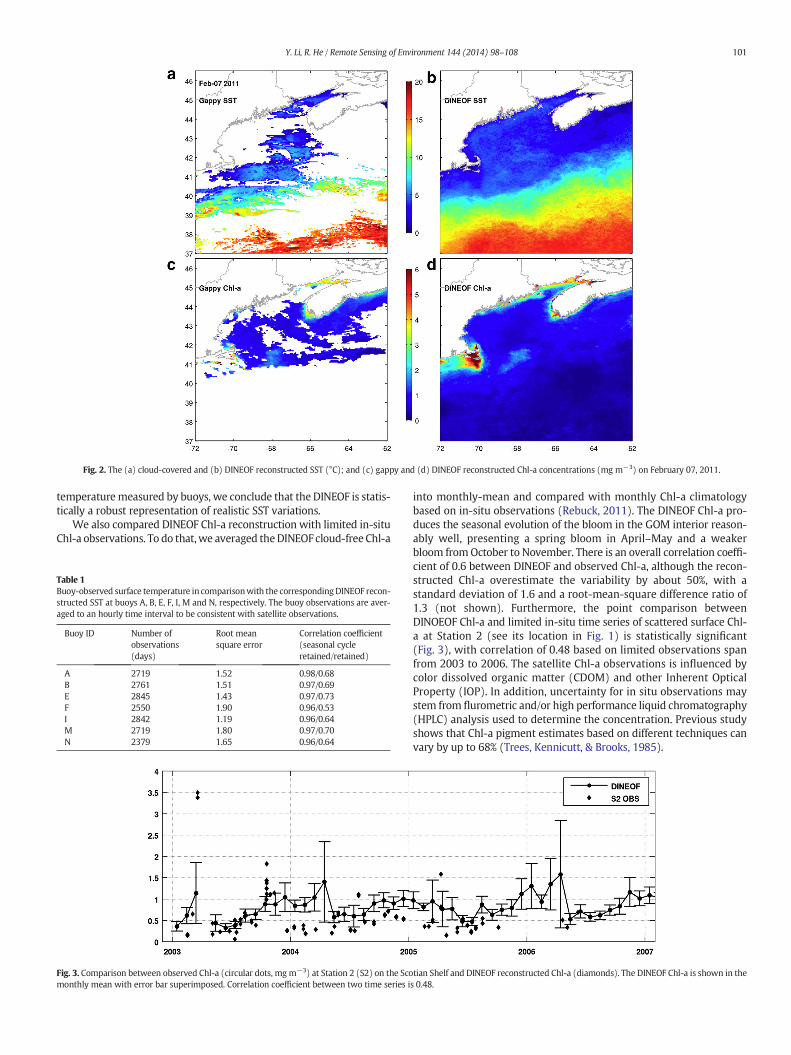
Fig. 2. The (a) cloud-covered and (b) DINEOF reconstructed SST (°C); and (c) gappy and (d) DINEOF reconstructed Chl-a concentrations (mg m−3) on February 07, 2011.

101Y. Li, R. He / Remote Sensing of Environment 144 (2014) 98–108

temperaturemeasured by buoys, we conclude that the DINEOF is statis-tically a robust representation of realistic SST variations.

We also compared DINEOF Chl-a reconstruction with limited in-situChl-a observations. To do that,we averaged theDINEOF cloud-free Chl-a

Table 1Buoy-observed surface temperature in comparisonwith the correspondingDINEOF recon-structed SST at buoys A, B, E, F, I, M and N, respectively. The buoy observations are aver-aged to an hourly time interval to be consistent with satellite observations.

Buoy ID Number ofobservations(days)

Root meansquare error

Correlation coefficient(seasonal cycleretained/retained)

A 2719 1.52 0.98/0.68B 2761 1.51 0.97/0.69E 2845 1.43 0.97/0.73F 2550 1.90 0.96/0.53I 2842 1.19 0.96/0.64M 2719 1.80 0.97/0.70N 2379 1.65 0.96/0.64

Fig. 3. Comparison between observed Chl-a (circular dots, mgm−3) at Station 2 (S2) on the Scomonthly mean with error bar superimposed. Correlation coefficient between two time series i

into monthly-mean and compared with monthly Chl-a climatologybased on in-situ observations (Rebuck, 2011). The DINEOF Chl-a pro-duces the seasonal evolution of the bloom in the GOM interior reason-ably well, presenting a spring bloom in April–May and a weakerbloom fromOctober to November. There is an overall correlation coeffi-cient of 0.6 between DINEOF and observed Chl-a, although the recon-structed Chl-a overestimate the variability by about 50%, with astandard deviation of 1.6 and a root-mean-square difference ratio of1.3 (not shown). Furthermore, the point comparison betweenDINOEOF Chl-a and limited in-situ time series of scattered surface Chl-a at Station 2 (see its location in Fig. 1) is statistically significant(Fig. 3), with correlation of 0.48 based on limited observations spanfrom 2003 to 2006. The satellite Chl-a observations is influenced bycolor dissolved organic matter (CDOM) and other Inherent OpticalProperty (IOP). In addition, uncertainty for in situ observations maystem from flurometric and/or high performance liquid chromatography(HPLC) analysis used to determine the concentration. Previous studyshows that Chl-a pigment estimates based on different techniques canvary by up to 68% (Trees, Kennicutt, & Brooks, 1985).

tian Shelf and DINEOF reconstructed Chl-a (diamonds). The DINEOF Chl-a is shown in thes 0.48.

102 Y. Li, R. He / Remote Sensing of Environment 144 (2014) 98–108

3.2. Monthly Climatology of SST and Chl-a

The reconstructed decade-long daily SST and Chl-a were temporallyaveraged to produce their respective monthly climatology for the region(Figs. 4 and 5). The SST shows a sinusoidal seasonal cycle, with persistentseasonalwarming trend fromwinter (March) to summer (August). Thereis a clear temperature contrast between the gulf water and the openocean water in spring and fall. The thermal difference reaches as highas ~4 °C between GOM and Slope Sea in August. The thermal front nearthe shelfbreak is however more visible in winter and spring months.Spatially, the Georges Bank, SS and eastern GOMhave lower temperaturecompared to the western GOM, which is in part a result of stronger tidalmixing and coast water advection from Scotian Shelf (Fig. 4).

Fig. 4. Long-term SST (°C) monthly mean climatology computed

Using a four-year SeaWiFs Chl-a data, Thomas et al. (2003) derived aseasonal cycle. Here we intend to quantify the annual cycle of Chl-a aswell but using a decadal-long time series. The climatological seasonalcycle of Chl-a (Fig. 5) shows larger spatial heterogeneity compared toSST. Overall, the Chl-a concentration is larger either in the coastal west-ern GOM or in the regions with stronger tidal signals, such as northernflank of Georges Bank and Bay of Fundy. Our results show similar sea-sonal features identified by Thomas et al. (2003). For example, 1)there are elevated Chl-a concentrations in nearshore waters andGeorges Bank in spring and fall bloom seasons. 2) The bloom in thedeep basin of GOM generally follows a canonical North Atlantic bloomseasonal cycle. There is low Ch-abloom in winter, an annual maximumin March–April, decreased concentration in summer, followed by a fall

from daily DINEOF SST reconstruction during 2003–2012.

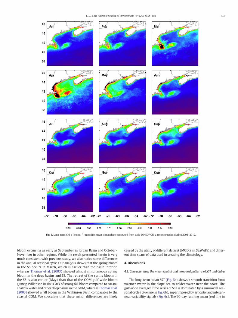
Fig. 5. Long-term Chl-a (mg m−3) monthly mean climatology computed from daily DINEOF Chl-a reconstruction during 2003–2012.

103Y. Li, R. He / Remote Sensing of Environment 144 (2014) 98–108

bloom occurring as early as September in Jordan Basin and October–November in other regions. While the result presented herein is verymuch consistent with previous study, we also notice some differencesin the annual seasonal cycle. Our analysis shows that the spring bloomin the SS occurs in March, which is earlier than the basin interior,whereas Thomas et al. (2003) showed almost simultaneous springbloom in the deep basins and SS. The retreat of the spring bloom inthe SS is also earlier (May) than that of the GOM gulf-wide bloom(June);Wilkinson Basin is lack of strong fall bloom compared to coastalshallowwater and other deep basins in the GOM,whereas Thomas et al.(2003) showed a fall bloom in the Wilkinson Basin comparable to thecoastal GOM. We speculate that these minor differences are likely

caused by theutility of different dataset (MODIS vs. SeaWiFs) and differ-ent time spans of data used in creating the climatology.

4. Discussions

4.1. Characterizing themean spatial and temporal patterns of SST and Chl-a

The long-term mean SST (Fig. 6a) shows a smooth transition fromwarmer water in the slope sea to colder water near the coast. Thegulf-wide averaged time series of SST is dominated by a sinusoidal sea-sonal cycle (blue line in Fig. 6b), superimposed by synoptic and interan-nual variability signals (Fig. 6c). The 60-day running mean (red line in

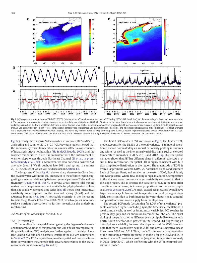
Fig. 6. (a) Long-term temporalmean of DINEOF SST (°C). (b) time series of domain-wide spatialmean SST during 2003–2012 (black line) and the seasonal cycle (blue line) associatedwithit. The seasonal cycle was derived by long-term averaging the daily snapshots during 2003–2012 that are on the same day of year, a similar approach as harmonic fitting but reserves sec-ondary peaks such as the Chl-a fall bloom. (c) Time series of domain-wide spatial mean SST anomalies (in gray) and its 60-day running mean (in red); (d) long-term temporal-mean ofDINEOF Chl-a concentration (mgm−3); (e) time series of domain-wide spatial mean Chl-a concentration (black line) and its corresponding seasonal cycle (blue line). (f) Spatial-averagedChl-a anomalies with seasonal cycle subtracted (in gray) and its 60-day running mean (in red); for both panels e and f, a natural logarithmic scale is applied to time series of Chl-a con-centration to offer better visualizations. (For interpretation of the references to color in this figure legend, the reader is referred to the web version of this article.)

104 Y. Li, R. He / Remote Sensing of Environment 144 (2014) 98–108

Fig. 6c) clearly shows warm SST anomalies in summer 2005 (~0.5 °C)and spring and summer 2010 (~0.7 °C). Previous studies showed thatthe anomalously warm temperature in summer 2005 is a consequenceof increased surface net heat flux (He & McGillicuddy, 2008), and thewarmer temperature in 2010 is coincident with the entrainment ofwarmer slope water through Northeast Channel (Li et al., in press;McGillicuddy et al., 2011). Moreover, we also noticed a positive SSTanomaly (over 1 °C) throughout late 2011 and spring to summer2012. The causes of which will be discussed in Section 4.2.

The long-term Chl-a (Fig. 6d) shows sharp decrease in Chl-a fromthe coastal water within the 100-m isobath to the offshore region, sug-gesting an inverse relationship between general pattern of Chl-a andba-thymetry (O'Reilly et al., 1987). In several areas, strong tidal mixingmakes more deep-ocean nutrient available for phytoplankton utiliza-tion. The spatially-averaged time series (Fig. 6f) shows clear interannualvariability superimposed on the seasonal spring (April) and fall(August) blooms (Fig. 6e). A noticeable scenario is the increasingtrend in the gulf-wide Chl-a from2003–2011, which requiresmore sub-surface nutrient observations to further investigate the underlyingmechanisms.

4.2. Modes of the variability in SST and Chl-a

4.2.1. SST variabilityTo better discern the spatial heterogeneity, the degree of coherence

and temporal evolution of temperature and Chl-afields, an empirical or-thogonal function (EOF) analysis was further applied to the daily, cloud-free DINEOF SST and Chl-a datasets. Details of the EOF are summarizedin Section 2. The EOF analysis then provides spatial and temporal func-tions derived from the anomaly field covariances relative to the spatialmean fields (as shown in Fig. 6a and d).

The first 3 EOF modes of SST are shown in Fig. 7. The first SST EOFmode accounts for the 92.43% of the total variance. Its temporal evolu-tion is overall dominated by an annual periodicity peaking in summerandwinter, as well as the interannual variability signal such as elevatedtemperature anomalies in 2005, 2010, and 2012 (Fig. 7b). The spatialvariation shows that SST has different phase in different region. As a re-sult of tidal rectification, the spatial EOF is highly coincident with M-2tidal amplitude distribution in the region. The magnitude of EOF1 isoverall larger in the western GOM, SS, Nantucket Islands and southernflank of Georges Bank, and smaller in the eastern GOM, Bay of Fundyand Georges Bank where tidal mixing is high. In addition, temperaturein the shallow water presents a larger variability compared to that inthe slope region. This is because the variation of SST, in the first orderone-dimensional sense, is inverse proportional to the water depth(e.g., He & Weisberg, 2003). As such, coastal ocean waters overall havelarger seasonal cycle. In contrast, temperature in the slope region staysfairly consistent due to both increase in water depth (heat content)and persistent warm water supply from the slope sea.

The second EOF mode (accounting for 1.24% of total variance) pre-sents combined signals including synoptic time-scale oscillations, aweak annual cycle, as well as interannual variability. PC2 reaches itspeak in May–July and its minimum December to February. The exacttiming of the peak varies in different years. A dipole-like feature withnorth–south orientation is present in the second EOF suggesting anout-of-phase variability between the slope sea and the GOM. We alsonote that there is a positive peak in 2008 and obvious negative peaksin summer 2010 and 2012. Thus, mode 2 is indeed an augmentationof the interannual variability signal in mode 1 for the GOM and SS. Incontrast, mode 2 provides a positive (negative) temperature anomalyin 2008 (2010/2012), which is offsetting with the SST interannual vari-ations in mode 1.

Fig. 7. Eigenfunctions (EOFs, °C, upper panels) and temporal evolution functions (PCs, lower panels) for thefirst three SSTmodes.White lines for EOF2 and EOF3 stand for the zero contourline. For each temporal evolution function, 60-day runningmean (pink) is plotted on top of daily analysis (gray). The percentage of SST variance accounted for by eachmode is also labeled.

105Y. Li, R. He / Remote Sensing of Environment 144 (2014) 98–108

The third EOFmode (accounting for 1.16% of total variance) presentsa feature with a more east–west orientation. It shows an inverse vari-ability between waters in continental slope where Labrador SlopeWater converges, forming a front between the slope area and watersin the SS and Georges Bank. The cores of positive and negative anoma-lies are centered in the coastal western GOM and continental slopesouth of SS respectively. The time evolution function (PC3) showsmore interannual variations instead of seasonal cycles. There also ap-pears to be a decrease in SST in the continental slope in 2008 and2011, when PC2 shows an increase in SST near the slope sea furthersouth. This suggests that the variations in the Scotian-shelf/slope and

Fig. 8. Same as Fig. 7, but for Chl-a. A natural logarithmic sca

warm slope open ocean further south may be decoupled during theseyears. The interaction between WSW and LSW has previously been ar-gued to perplex the hydrodynamics near Georges Bank and NortheastChannel (Smith, Houghton, Fairbanks, & Mountain, 2001).

4.2.2. Chl-a variabilityWe applied a natural logarithmic scale to the Chl-a field prior to the

EOF decomposition. Therefore the values shown in the EOFs are in logscale relative to the mean field (Fig. 8d).

The first EOFmode (accounting for 42.74% of total variance) is dom-inated by the seasonal bloom peaking in spring and fall over the GOM

le was applied to the Chl-a field before the EOF analysis.

106 Y. Li, R. He / Remote Sensing of Environment 144 (2014) 98–108

and the broader upstream region near the Scotian Shelf. The seasonalcycle associated with this EOF mode is larger in the eastern GOM andGeorges Bank. There stronger tidal mixing stirs up the water columnand bring the deeper nutrient upward, which in turn favors the phyto-plankton bloom. The spatial EOF separates the tidal-dominated shallowwater regimewith deep ocean basins in theGOM. In addition, the bloomsouth of the Great South Channel is out of phase with the seasonal cycleinside the GOM, a feature already demonstrated in Section 3.2. As such,mode 1 is a good representation of difference in the timing of the bloom.The out-of-phase seasonality betweenwaters in the GOM and the SlopeSea is consistent with previous studies. For example, Eslinger, O'Brien,and Iverson (1989) showed out-of-phase variability of bloom south ofGeorges Bank with GOM interior in 1979. Yoder et al. (2001) alsofound poor correlation in temporal evolution of Chl-a between GB andshelf region further south.

The second EOF mode (accounting for 10.48% of total variance)shows a seasonal cycle different from the first mode. It shows inverserelationship between shallow water over the entire Continental Shelfand slope sea further south. The time evolution function peaks in eachwinter and summer, maximizing in November–January andminimizingin June–August for the Continental Slope. There is also a secondarybloom in fall. Thus, mode 2 highlights evolutions of the deep-oceanbloomwhich is out-of-phase with the bloom in the GOM and upstreamregion, consistent with findings of Thomas et al. (2003) and Yoder et al.(2002). In addition,we postulate that thismode is likely associatedwithnutrient supply from the deep andwarm slope sea. The subsurface slopewater is nutrient rich, and thus offers important supplies from the sub-surface (e.g., Townsend, Rebuck, Thomas, Karp-Boss, & Gettings, 2010).The winter bloom in the warm slope of MAB consumes nutrient in thesouth, and hence restrict the bloom in the gulf interior.

Mode 3 (accounting for 5.04% of total variance) indicates a possibleinfluence of boundary inflow from the Scotian Shelf. The temporalevolution is highly oscillatory. The spatial EOF suggests an out-of-phase relationship between blooms in the western GOM and easternGOM and MAB. The advection of SSW delivers nutrient-poor surfacewater to the eastern GOMand Jordan Basin. In addition, the progressionof fresh surface SSW brings nutrient-poor water condition further

Fig. 9. (a) SST PC1 (black solid line) overlaid with normalized NCEP net heat flux time series (gline) and Chl-a PC2 (black dashed line) overlaid with daily NAO index (gray dashed line) and aShelf-slope frontal locations between 60 and63°W(gray shaded lines). In order to better represeto remove synoptic and intra-seasonal variations, following Venegas et al. (2008).

downstream, but has limited effect for the western GOM. As a result,the SSW inflow may have dampened the Chl-a bloom in the westernGOM, whereas water conditions continue to favor the bloom in thewestern GOM and New England shelf. Thus, the third mode is likely tobe related to the stability induced by ocean advection of low-salinitywater from the SS. Our finding is consistentwith Ji et al. (2007) showingthe significance of salinity in the SS in modulating the phytoplanktonbloom, and that the freshening in the eastern GOM has limited effecton the bloom condition in the western GOM. Overall, the first threemodes explain 59% of the total Chl-a variance. To analyze the remaining41% of the variability would require the analysis of high order modes.

4.2.3. Response of low-frequency SST/Chl-a variability to basin scale forcingThe low-frequency segments of SST and Chl-a signals have complex

variability in response to various atmospheric forcing at different time-scales. Here we focus on the SST variability in response to changes ofbasin-scale atmospheric forcing.

As discussed above, the first EOFmode of SST is dominated by a sea-sonal cycle. To compare with the surface forcing, we computed the sur-face net heat flux using NCEP reanalysis averaged over the researchdomain (Fig. 9a). The normalized net heat flux shows a similar peak asPC1, but leading the SST phase by 1–2 months. Lag correlation analysisconfirms that SST signal lags the surface heat flux by 1.9 months (57-days). The lag of SST cycle over the air–sea heat flux cycle, usually calledthe “oceanic heat storage phase lag” (g), has been documented in thepast. Li, Bye, Gallagher, and Cowan (2012) showed that with oceanadvection neglected, the lag time can be estimated based on aone-dimensional model. For 40°N, the lag time is estimated to be1.7 months, which is overall consistent with our result here. In additionto mode 1, the out-of-phase spatial relationship in both mode 2 andmode 3 suggested the interaction between coastal waters in the GOMand the Slope Sea, which is consistent earlier in the finding of Yoderet al.(2002) based on CZCS SST climatology. It has been found in previ-ous studies (Drinkwater, Mountain, & Herman, 1999; Pershing et al.,2001; Thomas et al., 2003) that the water properties near the NortheastChannel associatedwith slopewater oscillationsmay be related to largescale forcing signals such as the North Atlantic Oscillations (NAO). For

ray solid line) and its 57-day lagged rendition (gray dashed line). (b) SST PC2 (black solidnnual winter NAO index (gray dots). (c) SST PC3 (black) overlaid with normalized Scotiannt interannual variability, time series in (b) and (c) all underwent a 150-day runningmean

107Y. Li, R. He / Remote Sensing of Environment 144 (2014) 98–108

example, Thomas et al. (2003) analyzed the satellite SST during1997–2001 and relate the colder SST in 1998 to a positive NAO index.They argued that during positive NAO phase, less WSW from thesouth are entrained into the GOM, and subsequently led a regional SSTdrop in 1998.

Based on our longer time series in this study, we compared the PC2time series with both low-frequency NAO index andwinter NAO index.To retain only the low-frequency variability, both SST and Chl-a PC2 anddaily NAO indices are 150-day running-averaged, following the ap-proach used in Venegas et al. (2008). We found that the SST and Chl-aPC2 are overall in phase. There is also a good correlation between thePC2s and NAO index (Fig. 9b). Over the 10-year study period, the SSTPC2s is largely in-phase with NAO variability. The only exception is in2008, when a low NAO index seems to coincide with high SST/Chl-aPC indices. However, the winter NAO index is largely negative in 2008and 2009, suggesting that winter NAO index may provide more impacton the SST/Chl-a variability during this period.

To analyze the possible mechanism accounting for the SST mode 3,we compared the time series (shown in blue line) with the ScotianShelf-slope front location index produced by Bedford Institute ofOceanography, Canada (Fig. 9c). The strong coherence between thetwo signals suggests that mode 3 is likely dominated by the cross-shelf (east–west) displacement of the Shelf-Slope front near 60–63°W.We also noticed that the spatial variations in SST mode 3 are out ofphase between GOM and slope sea. A possible candidate mechanismis that when there is a subsurface intrusion of slope water into thegulf, SST in the continental slope decreases due to the overall heat lossfrom advection. In themeantime, there can be an increase in the SST in-side the gulf as a result of heat supply from the subsurface warm waterintrusion. It also shows that EOF can be used as an alternative tool toidentify the overall location of the SSW front.

In addition to SST,we also investigated the relationship between SSTand Chl-a and the linkage between the variability of Chl-a and large-scale forcing. No clear relationship was found between SST and Chl-aon interannual timescale for other major EOF modes except for mode2. The coincidence between SST and Ch-a variability in mode 2 suggeststhat the two variables are coupled during most years. Thomas et al.(2003) postulated that the coupling between SST and Chl-a as shownin PC2 is likely due to decreased inflow of nutrient-rich warm slopewaters from subsurface, which favors a weaker Chl-a bloom, as well asdecreased SST through vertical mixing. This was further evidenced bythe regime-shift of nutrient condition suggested by Townsend et al.(2010). Despite the coherence of PC2 in SST and Chl-a in 2009, 2010,and 2012, the two variables seem decoupled in other years such as2003, when negative SST anomaly in the GOM is coincident with posi-tive Chl-a concentration. The direct relationship between Chl-a andNAO is not as clear as that for SST PC2, suggesting that other mecha-nisms are responsible for the Chl-a interannual variability. The offshorenutrient flux, wind forcing, coastal riverine nutrient discharge, waterstratification, and upper trophic biomass are all possible factorsaccounting for Chl-a variations.

5. Summary and conclusion

The spatial and temporal variability of the SST and Chl-a was exam-ined using a decade long cloud-free DINEOF SST and Chl-a analysis. TheSST showed a sinusoidal seasonal cycle. Positive SST anomalies werepresent in 2005, 2010 and 2012 in response to the variations in surfaceheat flux. The first SST EOFmodewas dominated by an annual periodic-ity peaking in summer and winter, and the signal lags the surface netheat flux by ~50 days. Further analysis showed that the magnitude ofthe seasonal cycle at different locations in the GOM is a result of waterdepth, tidal rectification and heat flux redistribution. The second EOFmode started to include some synoptic time-scale oscillations, an annu-al cycle, as well as interannual variability. The PC2 reached its peak inMay–July and its minimum in December to February. A dipole-like

feature with north–south orientation was present in the second spatialEOF, which suggests an out-of-phase variability between waters inSlope Sea and in the GOM. It underscored the interactions betweenbroad GOM and the slope sea region in response to large scale forcingvariability (such as the North Atlantic Oscillation). The third modeshowed more interannual variations instead of seasonal cycles, whichis likely responding to the Scotian Shelf-Slope frontal dynamics.

Chl-a variability was generally dominated by a spring bloom with asecondary fall bloom in the GOM. The different timing in the springand fall blooms was identified. There is an overall increasing trend insurface Chl-a bloom during 2003–2011, and decreasing thereafter. Thefirst EOF mode showed stronger seasonal variability in the area withstronger tidal forcing. The second mode presented an out-of-phasedrelationship in the waters between GOM and the open ocean slopesea, and is highly in phase with the second mode of SST. Therefore,mode 1 and mode 2 represented responses of Chl-a bloom to bothlocal and atmospheric forcing, both of which may have significant im-pact on higher trophic cascade such as shrimp hatching processes(Koeller et al., 2009). Moreover, the highly in-phase variation betweenSST and Chl-a PC2s and NAO index suggests a possible linkage betweenatmospheric forcing and coupled ocean physical–biological interaction.Mode 3 was likely associated with the effect of fresh water advectedfrom the upstream on the bloom in the coastal GOM. In addition tothe delivery of nutrient-poor ocean condition to the eastern GOM, thefresh SSW helps to establish stratification that impedes the nutrient up-take in the easternGOM. The salinity impact, however, has limited effecton the western GOM and phytoplankton bloom further downstream(Ji et al., 2007) in the western GOM.

The DINEOF analysis herein provides a useful dataset for investigat-ing the spatial and temporal variability of the coastal SST and Chl-a. Wenote however that satellite remote sensing observes only the near sur-face layer of the ocean. Their data are short by climate standards(Antoine, Morel, Gordon, Banzon, & Evans, 2005) because they cannotaddress physical and biological properties over the entire water column(Platt & Herman, 1983). The chlorophyll can have a peak at subsurface,representing a phytoplankton biomassmaximum that occurs at a depthwhere both light and nitrate availability allow net growth of the popu-lation (Holligan et al., 1984). High concentration of surface pigmentcould come from either 1) biomass enhancement stimulated by the in-troduction of nutrient into surface euphotic layer, or 2) vertical advec-tion of colored materials from their subsurface maxima (He et al.,2010; McGillicuddy, Kosnyrev, Ryan, & Yoder, 2001). The trend of Chl-a variation in the recent year is likely associated with the nutrient re-gime shift in the GOM (Townsend et al., 2010). Finally, the satellite-derived coastal ocean color is subject to contamination by CDOM andsuspended sediment, the composite of which is largely unknown. Assuch, more subsurface Chl-a and nutrient information are needed tobetter understand the dynamic of phytoplankton blooms and their link-age with climate signals.

Acknowledgment

We thank NASA GSFC for servingMODIS SST and Chl-a data. We arealso grateful to NERACOOS and AZMP program for providing in-situbuoy temperature and chlorophyll data online. Research support pro-vided by NOAA grants: NA06NOS4780245 and NA11NOS0120033,NASA grants: NNX10AU06G, NNX12AP84G, and NNX13AD80G aremuch appreciated.

References

Alvera-Azcárate, A., Barth, A., Beckers, J. -M., & Weisberg, R. H. (2007). Multivariatereconstruction of missing data in sea surface temperature, chlorophyll and windsatellite fields. Journal of Geophysical Research, 112, C03008. http://dx.doi.org/10.1029/2006JC003660.

108 Y. Li, R. He / Remote Sensing of Environment 144 (2014) 98–108

Alvera-Azcárate, A., Barth, A., Rixen, M., & Beckers, J. -M. (2005). Reconstruction of incom-plete oceanographic data sets using Empirical Orthogonal Functions. Application tothe Adriatic Sea. Ocean Modelling, 9, 325–346.

Alvera-Azcárate, A., Barth, A., Sirjacobs, D., & Beckers, J. -M. (2009). Enhancing temporalcorrelations in EOF expansions for the reconstruction of missing data using DINEOF.Ocean Science, 5, 475–485.

Antoine, D., Morel, A., Gordon, H. R., Banzon, V. F., & Evans, E. H. (2005). Bridging oceancolor observations of the 1980s and 2000s in search of long-term trends. Journal ofGeophysical Research, 110. http://dx.doi.org/10.1029/2004JC002620.

Beckers, J. -M., Barth, A., & Alvera-Azcarate, A. (2006). DINEOF reconstruction of cloudedimages including error maps. Application to the Sea Surface Temperature aroundCorsican Island. Ocean Science, 2(2), 183–199.

Bigelow, H. B. (1927). Physical oceanography of the Gulf of Maine. Fisheries Bulletin, 40,511–1027.

Bisagni, J. J., & Smith, P. C. (1998). Eddy-induced flow of Scotian Shelf water across North-east Channel, Gulf of Maine. Continental Shelf Research, 18, 515–539.

Chaudhuri, A., Gangopadhyay, A., & Bisagni, J. J. (2009). Interannual variability of GulfStream warm-core rings in response to the North Atlantic Oscillation. ContinentalShelf Research, 29(7), 856–869 (15 April 2009).

Churchill, J. H., Pettigrew, N. R., & Signell, R. P. (2005). Structure and variability of theWestern Maine Coastal Current. Deep Sea Research, Part II, 52(19–21), 2392–2410.

Drinkwater, K. F., Mountain, D. B., & Herman, A. (1999). Variability in the slope waterproperties off eastern North America and their effects on the adjacent shelves. ICESCM, 8, 26.

Eslinger, D. L., O'Brien, J. J., & Iverson, R. L. (1989). EOF analysis of cloud contaminatedcoastal zone color scanner images of northeastern North American coastal waters.Journal of Geophysical Research, 94, 10884–10890.

Garrett, C. (1972). Tidal resonance in the Bay of Fundy and Gulf of Maine. Nature, 238,441–443.

He, R., Chen, K., Moore, T., & Li, M. (2010). Mesoscale variations of sea surface temperatureand ocean color patterns at the Mid-Atlantic Bight shelfbreak. Geophysical ResearchLetters. http://dx.doi.org/10.1029/2010GL043067.

He, R., & McGillicuddy, D. J. (2008). Gulf of Maine circulation and harmful algal bloom inSummer 2005 — Part 1: In-situ observation. Journal of Geophysical Research, 113,C07039. http://dx.doi.org/10.1029/2007JC004691.

He, R., McGillicuddy, D. J., Smith, K. W., Lynch, D. R., Stock, C. A., & Manning, J. P. (2005).Data assimilative hindcast of the Gulf of Maine coastal circulation. Journal ofGeophysical Research, 110. http://dx.doi.org/10.1029/2004JC002807 (C10, C10011).

He, R., & Weisberg, R. H. (2003). West Florida shelf circulation and temperature budgetfor 1998 fall transition. Continental Shelf Research, 23(8), 777–800.

He, R., Weisberg, R. H., Zhang, H., Muller-Karger, F. E., & Helber, R. W. (2003). A cloud freesatellite-derived, sea surface temperature analysis for the West Florida Shelf.Geophysical Research Letters, 30(15), 1811. http://dx.doi.org/10.1029/2003GL017673.

Herman, A. W., Sameoto, D.D., Shunnian, C., Mitchell, M. R., Petrie, B., & Cochrane, N.(1991). Sources of zooplankton on the Nova Scotia shelf and their aggregations with-in deep shelf basins. Continental Shelf Research, 11, 211–238.

Holligan, P.M., Balch, W. M., & Yentsch, C. M. (1984). The significance of subsurface chloro-phyll, nitrite and ammoniummaxima in relation to nitrogen for phytoplankton growthin stratified waters of the Gulf of Maine. Journal of Marine Research, 42, 1051–1073.

Ji, R., Davis, C., Chen, C., Townsend, D., Mountain, D., & Beardsley, R. (2007). Influence ofocean freshening on shelf phytoplankton dynamics. Geophysical Research Letters, 34,L24607. http://dx.doi.org/10.1029/2007GL032010.

Koeller, P., et al. (2009). Basin-scale coherence in phenology of shrimps and phytoplank-ton in the North Atlantic Ocean. Science, 324(5928), 791–793.

Li, C. -L., Bye, J. A. T., Gallagher, S. J., & Cowan, T. (2012). Annual sea surface temperaturelag as an indicator of regional climate variability. International Journal of Climatology.http://dx.doi.org/10.1002/joc.3587.

Li, Y., He, R., & McGillicuddy, D. J. (2013). Seasonal and interannual variability in Gulf ofMaine hydrodynamics: 2002–2011. Deep-Sea Research II, in press (http://dx.doi.org/10.1016/j.dsr2.2013.03.001).

Limeburner, R., & Beardsley, R. C. (1996). Near-surface recirculation over Georges Bank.Deep Sea Research II, 43, 1547–1574.

Luerssen, R. M., Thomas, A.C., & Hurst, J. (2005). Relationships between satellite-measured thermal features and Alexandrium-imposed toxicity in the Gulf of Maine.Deep Sea Research, Part II, 52, 2656–2673.

Lynch, D. R., Holboke, M. J., & Maimie, C. E. (1997). The Maine coastal current: Springclimatological circulation. Continental Shelf Research, 17, 605–639.

Lynch, D. R., Ip, J. T. C., Naimie, C. E., &Werner, F. E. (1996). Comprehensive coastal circulationmodel with application to the Gulf of Maine. Continental Shelf Research, 16(7), 875–906.

McGillicuddy, D. J., Kosnyrev, V. K., Ryan, J. P., & Yoder, J. A. (2001). Covariation ofmesoscale ocean color and sea surface temperature patterns in the Sargasso Sea.Deep-Sea Research II, 48, 1823–1836.

McGillicuddy, D. J., Townsend, D.W., He, R., Keafer, B.A., Kleindinst, J. L., Li, Y., et al. (2011).Suppression of the 2010 Alexandriumfundyense bloom by changes in physical, bio-logical, and chemical properties of the Gulf of Maine. Limnology and Oceanography,56(6), 2411–2426.

Miles, T., & He, R. (2010). Seasonal surface ocean temporal and spatial variability of theSouth Atlantic Bight: Revisiting with MODIS SST and Chl-a imagery. ContinentalShelf Research. http://dx.doi.org/10.1016/j.csr.2010.08.016.

Miles, T. N., He, R., & Li, M. (2009). Characterizing the South Atlantic Bight seasonal variabil-ity and cold water event in 2003 using a daily cloud-free SST and chlorophyll analysis.Geophysical Research Letters, 36, L02604. http://dx.doi.org/10.1029/2008GL036393.

O'Reilly, J. E., Evans-Zetlin, C., & Busch, D. A. (1987). Primary production. In R. H. Backus(Ed.), Georges Bank (pp. 221–233). Cambridge, MA: MIT Press.

O'Reilly, J. E., & Busch, D. A. (1984). Phytoplankton primary production on the northwest-ern Atlantic shelf. Rapports et procès-verbaux desréunions, 183, 255.

Pershing, A. J., Greene, C. H., Hannah, C., Sameoto, D., Head, E., Mountain, D., et al. (2001).Oceanographic responses to climate in the Northwest Atlantic.Oceanography, 14, 76–82.

Pettigrew, N. R., Churchill, J. H., Janzen, C. D., Mangum, L. J., Signell, R. P., Thomas, A.C., et al.(2005). The kinematic and hydrographic structure of the Gulf of Maine coastal cur-rent. Deep Sea Research, Part II, 52(19–21), 2369–2391.

Pettigrew, N. R., Townsend, D. W., Xue, H., Wallinga, J. P., Brickey, P. J., & Hetland, R. D.(1998). Observations of the Eastern Maine Coastal Current and its offshore exten-sions. Journal of Geophysical Research, 103(30), 623–640.

Platt, T., & Herman, A. W. (1983). Remote sensing of phytoplankton in the sea:Surface-layer chlorophyll as an estimate of water column chlorophyll and primaryproduction. International Journal of Remote Sensing, 4(2), 343–351.

Rebuck, N. D. (2011). Nutrient distributions in the Gulf of Maine: An analysis of spatial andtemporal patterns of dissolved inorganic nitrate and silicate. PhD Dissertation. Orono:University of Maine.

Ryan, J. P., Yoder, J. A., & Cornillon, P. C. (1999). Enhanced chlorophyll at the shelfbreak ofthe mid-Atlantic Bight and Georges Bank during the spring transition. Limnology andOceanography, 44, 1–11.

Sirjacobs, D., Alvera-Azcárate, A., Barth, A., Lacroix, G., Park, Y., Nechad, B., et al. (2011).Cloud filling of ocean colour and sea surface temperature remote sensing productsover the Southern North Sea by the Data Interpolating Empirical Orthogonal Func-tions methodology. Journal of Sea Research, 65(1), 114–130. http://dx.doi.org/10.1016/j.seares.2010.08.002.

Smith, P. C. (1983). The mean and seasonal circulation off southeast Nova Scotia. Journalof Physical Oceanography, 13, 1034–1054.

Smith, P. C., Houghton, R. W., Fairbanks, R. G., & Mountain, D.G. (2001). Interannual var-iability of boundary fluxes and water mass properties in the Gulf of Maine and onGeorges Bank: 1993–1997. Deep-Sea Research II, 48, 37–70.

Thomas, A.C., Townsend, D.W., &Weatherbee, R. (2003). Satellite-measured phytoplank-ton variability in the Gulf of Maine. Continental Shelf Research, 23, 971–989. http://dx.doi.org/10.1016/S0278-4343(03)00086-4.

Thomas, A.C., Weatherbee, R., Xue, H., & Liu, G. (2010). Interannual variability of shellfishtoxicity in the Gulf of Maine: Time and space patterns and links to environmentalvariability. Harmful Algae, 9, 458–480. http://dx.doi.org/10.1016/j.hal.2010.03.002.

Townsend, D.W., Cammen, L. M., Holligan, P.M., Campbell, D. E., & Pettigrew, N. R. (1994).Causes and consequences of variability in the timing of spring phytoplankton blooms.Deep-Sea Research I, 41, 747–765.

Townsend, D. W., Rebuck, N. D., Thomas, M.A., Karp-Boss, L., & Gettings, R. M. (2010).A changing nutrient regime in the Gulf of Maine. Continental Shelf Research, 30, 820–832.

Townsend, D. W., & Thomas, A.C. (2001). Winter–Spring Transition of phytoplankton chlo-rophyll and inorganic nutrients on Georges Bank. Deep-Sea Research II, 48, 199–214.

Townsend, D. W., & Thomas, M. (2002). Springtime nutrient and phytoplankton dynam-ics on Georges Bank. Marine Ecology — Progress Series, 228, 57–74.

Trees, Charles C., Kennicutt, Mahlon C., II, & Brooks, James M. (1985). Errors associatedwith the standard fluorimetric determination of chlorophylls and phaeopigments.Marine Chemistry, 17(1), 1–12.

Ullman, D. S., & Cornillon, P. C. (1999). Satellite‐derived sea surface temperature fronts onthe continental shelf off the northeast US coast. Journal of Geophysical Research:Oceans (1978–2012), 104(C10), 23459–23478.

Venegas, R. M., Strub, P. T., Beier, E., Letelier, R., Thomas, A.C., Cowles, T., et al. (2008).Satellite-derived variability in chlorophyll, wind stress, sea surface height, and tem-perature in the northern California Current System. Journal of Geophysical Research,113, C03015. http://dx.doi.org/10.1029/2007JC004481.

Volpe, G., Buongiorno Nardelli, B., Cipollini, P., Santoleri, R., & Robinson, I. S. (2012). Sea-sonal to interannual phytoplankton response to physical processes in the Mediterra-nean Sea from satellite observations. Remote Sensing of Environment, 117, 223–235.http://dx.doi.org/10.1016/j.rse.2011.09.020.

Xue, H., Chai, F., & Pettigrew, N. R. (2000). A model study of the seasonal circulation in theGulf of Maine. Journal of Physical Oceanography, 30(5), 1111–1135.

Yoder, J. A., O'Reilly, J. E., Barnard, A. H., Moore, T. S., & Ruhsam, C. M. (2001). Variability incoastal zone color scanner (CZCS) chlorophyll imagery of oceanmarginwaters off theUS East Coast. Continental Shelf Research, 21, 1191–1218.

Yoder, J. A., Schollaert, S., & O'Reilly, J. E. (2002). Climatological phytoplankton chlorophylland sea surface temperature patterns in continental shelf and slope waters off thenortheast US Coast. Limnology and Oceanography, 47, 672–682.

Zhao, Y., & He, R. (2012). Characterizing the Gulf of Mexico SST and ocean color variabilityusing a cloud-free satellite data analysis. Remote Sensing Letters, 3(8), 697–706.