Remote Interactive Direct Volume Rendering of AMR Data

Oliver Kreylos∗ Gunther H. Weber† E. Wes Bethel‡ John M. Shalf‡ Bernd Hamann∗

Kenneth I. Joy∗

Abstract

We describe a framework for direct volume rendering (DVR)of adaptive mesh refinement (AMR) data that operates di-rectly on the hierarchical AMR grid structure, without theneed to resample data onto a single uniform rectilinear grid.The framework can be used for a range of renderers op-timized for particular hardware architectures: a hardware-assisted renderer for single-processor graphics workstations,a parallel hardware-assisted renderer for clusters of graph-ics workstations or multi-CPU graphics workstations, and amassively parallel software-only renderer for supercomput-ers. It is also possible to use the framework for distributedrendering to visualize data sets only accessible by remoterendering servers. By exploiting the multiresolution struc-ture of AMR data, the hardware-assisted renderers can ren-der large data sets at interactive rates, even if data is storedremotely.

CR Categories: K.6.1 [Management of Computing andInformation Systems]: Project and People Management—Life Cycle

Keywords: Interactive, Direct Volume Rendering, Mul-tiresolution, Adaptive Mesh Refinement Data

1 Introduction

Adaptive Mesh Refinement (AMR) [1, 2, 3] is a grid gen-eration approach used to discretize the physical domain fornumerical simulation. The discretization is adapted to thevarying complexity of geometry or dependent physical vari-ables. AMR is a highly efficient technique supporting the useof higher-resolution meshes in regions of greater complex-ity. AMR technology is used, for example, in ComputationalFluid Dynamics (CFD) simulations, where small regions ofturbulence have to be resolved finely, and in astrophysicalsimulations, where scales can span several orders of magni-tude.

AMR methods represent a computational domain as a hi-erarchy of grids of different cell sizes and possibly differentstructures [4]. While there exist several different types ofAMR data for different application areas, our rendering al-gorithm focuses on the Berger–Colella flavor of AMR andrequires data sets to satisfy the following properties:

• All grids are Cartesian.

• Grids in the same hierarchy level, i.e., grids having thesame cell size, do not overlap.

∗Center for Image Processing and Integrated Comput-ing (CIPIC), University of California, Davis†Fachbereich Informatik, Universitat Kaiserslautern‡Visualization Group, Ernest Orlando Lawrence Berkeley Na-

tional Laboratory

• All refinement ratios, i.e., all ratios of cell sizes betweenadjacent hierarchy levels, are integers (typically two orfour).

• Grid cells are never partially refined.

An example of a 2D AMR hierarchy with three levels and auniform refinement ratio of two is shown in Figure 1. Fig-ure 2 shows the 3D grid structure of a real AMR data set.

(a) (b)

Figure 1: Three-level AMR hierarchy with a uniform refine-ment ratio of two. Grid boundaries are denoted by bold lines.All hierarchy levels consist of two grids. Note that finer gridscan cross boundaries between coarser grids. (a) View offinest-resolution cells only. (b) “Exploded” view of AMR hi-erarchy. Shaded cells are “hidden” by finer-resolution grids.

Though AMR methods are advantageous for the simu-lation of certain physical phenomena, they pose problemswhen one wants to visualize simulation results. Most ex-isting visualization algorithms cannot handle AMR data di-rectly, and the strategy used in the past was to resampleAMR data onto a uniform grid (typically at the finest res-olution present in a given AMR hierarchy). This approachdoes not work well, because the AMR grid structure – ofteninteresting itself – is lost, and, due to the AMR data’s multi-ple resolution levels, resampled data tends to be too large tosupport efficient visualization. Considering a 3D AMR dataset containing 16 levels of resolution (common in astrophys-ical simulations) with a uniform refinement ratio of two, a

resampled grid would consist of at least(215)3

cells.

Figure 2: Argon Bubble data set. AMR hierarchy consistingof three levels, with refinement ratios of two and four, and528 grids in total. Image shows AMR grid structure blendedinto volume rendering.

It is therefore necessary to develop visualization algo-rithms that can handle AMR data directly and exploit the

structure of AMR data for visualization. AMR hierarchiesare a collection of Cartesian grids, and efficient visualiza-tion techniques exist for those; and AMR hierarchies are in-herently multiresolutional. Even though coarser grids maypartially be overlaid by finer ones, the “hidden” cells stillcontain meaningful data, albeit at a lower resolution. Thus,it is possible to visualize low-resolution approximations ofthe complete AMR hierarchy by ignoring some of the finerlevels.

Due to the size of typical AMR data sets (gigabytes toterabytes) it is often not practical to move a data set to auser’s machine for interactive visualization. Therefore, anAMR visualization system should support remote render-ing. In such a distributed system, the rendering takes placeon the machine that generated and/or stores the data, anduser interaction and display take place on the user’s ma-chine. Remote rendering saves the cost of transmitting largeamounts of data to a user’s machine, and enables the use ofhigh-performance hardware located at a remote site. It ishighly desirable that remote rendering is interactive, even ifa user’s machine is connected to the rendering server via theInternet.

We present an interactive volume visualization algorithmthat reads an AMR data set in its native file format, splitsthe AMR hierarchy into a set of Cartesian grid patcheson-the-fly, renders those patches using standard DVR al-gorithms, and composites the results into a final image. Thealgorithm can easily be adapted to several machine architec-tures by replacing the core rendering module, and it can beparallelized by scattering grid patches across several CPUsfor independent rendering and gathering partial images dur-ing compositing. We have implemented (i) a single-CPU,hardware-assisted renderer for smaller data sets stored ona user’s desktop computer; (ii) remote, parallel, hardware-assisted renderers for clusters of PC-based graphics work-stations or high-end multi-pipe graphics workstations; and(iii) a remote, massively parallel, software-only renderer forsupercomputers. The “thin client” for remote renderingcould be implemented as a web browser applet.

2 Related Work

DVR algorithms have been an active area of research for atleast the last decade [5]. Many DVR algorithms are designedfor Cartesian grids, and most can be used for the core render-ing module in our visualization systems, e. g., ray casting [6],cell projection [7], shear-warp transform [8], and hardware-assisted texture-based volume rendering [10, 11, 12]. SomeDVR algorithms suitable for unstructured grids, e. g., cellprojection [7], its polygonal approximation [13], and incre-mental slicing [14], can also be applied to AMR hierar-chies [15].

3 Volume Rendering AMR Data

We decided not to develop DVR techniques specific for AMRdata, but instead to homogenize a given AMR data set suchthat it can be rendered with existing DVR algorithms forCartesian grids. This strategy allows us to adapt our ren-derer to different machine architectures by merely replacingthe core rendering module. We split the process of renderingAMR data into the following four steps:

(1) Grid homogenization. Most DVR algorithms are op-timized for Cartesian grids. Considering this fact, in

the first step, we split an AMR hierarchy into a set ofnon-overlapping Cartesian grid patches. This step isperformed only once, on-the-fly, while loading an AMRdata set’s grid structure, and does not involve resam-pling. This step typically requires only a fraction of asecond.

(2) Domain decomposition. For parallel rendering, thegrid patches have to be distributed across processingnodes for rendering. Nodes have to load only thoseparts of an AMR data set that they are assigned to,allowing us to render large AMR data sets that do notfit into memory on a single processing node. We haveinvestigated two different methods to perform load bal-ancing during domain decomposition that do not re-quire communication between processing nodes.

(3) Back-to-front grid patch rendering. The grid pat-ches assigned to a processing node are rendered us-ing standard DVR algorithms. Our current software-only renderer uses a simple cell projection algorithm,whereas the hardware-assisted renderers employ the3D texture mapping capabilites of high-end graph-ics workstations or current consumer-level graphicsboards [10, 11, 12].

(4) Image compositing. For parallel rendering, the par-tial images generated independently by the processingnodes have to be composited into a single final image.Currently, we use a simple binary-tree based composit-ing algorithm. More advanced parallel compositing al-gorithms, e. g., binary swap [19], will be investigated inthe future.

The following sections describe these steps in more detail.Since Steps 2 and 4 only apply to the parallel renderingalgorithm, and since they are closely related to each other,they are treated together in Section 3.3.

3.1 Grid Homogenization

For rendering, our algorithm splits an AMR data set into aset of non-overlapping grid patches. A grid patch is definedas a rectangular subgrid of a single grid in an AMR hierarchy.This definition implies that all cells in a grid patch are ofidentical size, and the grid patch’s data belongs to a singlegrid and is therefore stored in a single contiguous region ofmemory. These properties ensure that any grid patch canbe rendered by standard DVR algorithms. The set of gridpatches is constructed in such a way that it covers the entiredomain of the AMR data set, and that it represents the finestresolution existing at any point. We call the process of tilinga data set’s domain with grid patches grid homogenization.

Figure 3: Three overlapping grids from two different hierar-chy levels split into grid patches. Boundaries between gridsare denoted by bold lines; individual grid patches are de-noted by different textures.

Grid homogenization is performed by overlaying a kd-tree [17] onto the domain of an AMR data set, such that

each grid patch in the homogenized AMR data set is rep-resented by one kd-tree leaf. Initially, the tree consists of asingle leaf representing the entire domain. Grids from theAMR hierarchy are subsequently inserted one-by-one, in or-der of increasing resolution1. Each grid to be inserted isimplicitly split into a set of grid patches by existing interiorkd-tree nodes while traversing the tree downwards, see Fig-ure 4(a–b). When an interior node is completely containedinside one of those patches, it and its subtree are replacedby a leaf representing that patch. If, on the other hand, anexisting kd-tree leaf is partially overlaid by a grid patch, thatleaf is recursively split into a set of non-overlapped patchesand a single overlaid patch. The latter is then replaced bythe new higher-resolution grid patch, see Figure 4 (c). Thecomplete kd-tree generated by homogenizing the AMR dataset from Figure 1 is shown in Figure 5.

(a) (b)

(c)

Figure 4: Inserting grid into kd-tree generated during gridhomogenization. (a) Kd-tree structure before insertion ofdashed grid. (b) Inserted grid split into patches after travers-ing existing tree. (c) New kd-tree generated by splittingpartially overlaid leaves.

(a) (b)

(c)

Figure 5: Homogenizing AMR data set from Figure 1.(a) Kd-tree after insertion of both level–0 grids. (b) Treeafter insertion of both level–1 grids. (c) Final tree after inser-tion of both level–2 grids. Newly inserted grids are shaded.

3.2 Back-to-front Grid Patch Rendering

The idea behind our approach is to render each of the gridpatches generated during homogenization independently, us-ing a standard DVR algorithm, and then to composite theindividual results. The compositing step is especially simpleif grid patches are rendered in back-to-front order [16]. If

1Grids inside the same hierarchy level do not need to be in-serted in any particular order.

one grid patch has been rendered as an RGB image withα-channel, it can be composited into the image representingall patches behind it by performing an “over” operation [16],either performed in software or in hardware as an α-blendingoperation. In the special case of a texture-mapping basedhardware-assisted DVR algorithm [10, 11, 12], compositingcan be performed implicitly by rendering all grid patchesinto the same frame buffer.

The view-independent kd-tree generated during grid ho-mogenization is also used to efficiently enumerate all gridpatches in correct rendering order. An interior kd-tree nodecan be interpreted as a plane dividing the node’s domaininto two regions, with one child node representing each re-gion and no node in either subtree intersecting the dividingplane. This interpretation leads to a directed depth-firsttraversal scheme for the homogenizing kd-tree: At each in-ternal node, the viewpoint is compared with the node’s di-viding plane, and the subtree corresponding to the region“behind” the plane (as seen from the viewpoint) is traversedfirst; the other region is traversed second. Since the tworegions are separated by the dividing plane, no grid patchrendered during the first traversal can occlude any grid patchrendered during the second traversal. By applying this steprecursively we obtain a unique back-to-front ordering of allgrid patches in the kd-tree. This approach leads to correctcompositing, even if the viewpoint is inside the AMR dataset’s domain. Note that the ordering algorithm is basedsolely on the viewpoint and is independent of viewing direc-tion. The grid patch order imposed by traversing the kd-treefrom Figure 5 is shown in Figure 6.

2

3

45

6

9

1011

7

13

1417 16

15

18

12

8 1

Figure 6: Grid patch order imposed by traversing the homog-enizing kd-tree from Figure 5 in back-to-front order (view-point indicated by “×”).

Once the grid patches are ordered correctly, they arepassed to the core rendering module individually. Ourcurrent implementation contains two different renderers:one is a standard cell-projection renderer [7] intended tobe used on massively parallel supercomputers, the otherone is a texture-mapping based, hardware-assisted ren-derer [10, 11, 12] for single or clustered PC-based, desktopgraphics workstations using commodity graphics hardware(NVidia GeForce3) or high-end graphics workstations (SGIOnyx2 with multiple Infinite Reality2 pipes).

3.2.1 Hardware-assisted Rendering

A typical 3D texture-mapping based volume renderer definesa 3D array of scalar data as a single intensity-only 3D textureand the accompanying transfer function as a color table map-ping from intensity to (RGB, α) tuples. The renderer sub-sequently visualizes the volume by generating and renderingtextured slices inside the data’s domain. Typically, slices arepolygonal intersections between equidistant view-orthogonalplanes and the data’s domain, see Figure 7. Slices are pro-cessed in back-to-front order, texture-mapped by generat-ing appropriate texture coordinates for their vertices, and

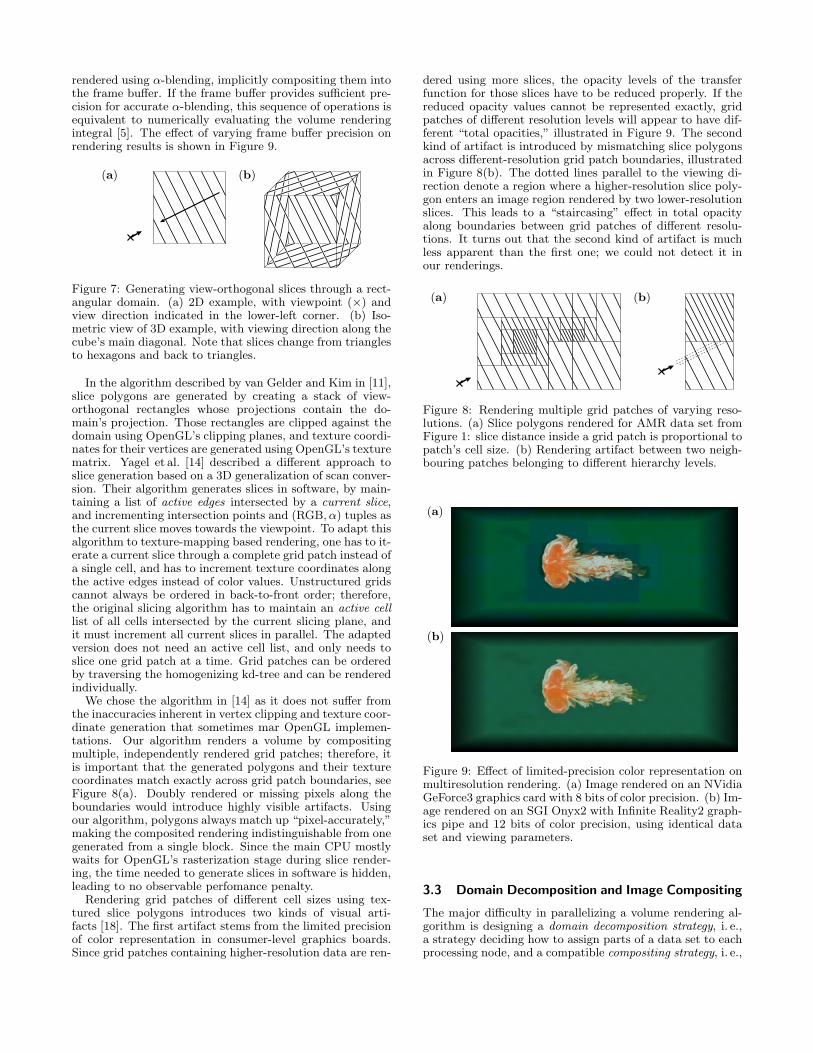
rendered using α-blending, implicitly compositing them intothe frame buffer. If the frame buffer provides sufficient pre-cision for accurate α-blending, this sequence of operations isequivalent to numerically evaluating the volume renderingintegral [5]. The effect of varying frame buffer precision onrendering results is shown in Figure 9.

(a) (b)

Figure 7: Generating view-orthogonal slices through a rect-angular domain. (a) 2D example, with viewpoint (×) andview direction indicated in the lower-left corner. (b) Iso-metric view of 3D example, with viewing direction along thecube’s main diagonal. Note that slices change from trianglesto hexagons and back to triangles.

In the algorithm described by van Gelder and Kim in [11],slice polygons are generated by creating a stack of view-orthogonal rectangles whose projections contain the do-main’s projection. Those rectangles are clipped against thedomain using OpenGL’s clipping planes, and texture coordi-nates for their vertices are generated using OpenGL’s texturematrix. Yagel et al. [14] described a different approach toslice generation based on a 3D generalization of scan conver-sion. Their algorithm generates slices in software, by main-taining a list of active edges intersected by a current slice,and incrementing intersection points and (RGB, α) tuples asthe current slice moves towards the viewpoint. To adapt thisalgorithm to texture-mapping based rendering, one has to it-erate a current slice through a complete grid patch instead ofa single cell, and has to increment texture coordinates alongthe active edges instead of color values. Unstructured gridscannot always be ordered in back-to-front order; therefore,the original slicing algorithm has to maintain an active celllist of all cells intersected by the current slicing plane, andit must increment all current slices in parallel. The adaptedversion does not need an active cell list, and only needs toslice one grid patch at a time. Grid patches can be orderedby traversing the homogenizing kd-tree and can be renderedindividually.

We chose the algorithm in [14] as it does not suffer fromthe inaccuracies inherent in vertex clipping and texture coor-dinate generation that sometimes mar OpenGL implemen-tations. Our algorithm renders a volume by compositingmultiple, independently rendered grid patches; therefore, itis important that the generated polygons and their texturecoordinates match exactly across grid patch boundaries, seeFigure 8(a). Doubly rendered or missing pixels along theboundaries would introduce highly visible artifacts. Usingour algorithm, polygons always match up “pixel-accurately,”making the composited rendering indistinguishable from onegenerated from a single block. Since the main CPU mostlywaits for OpenGL’s rasterization stage during slice render-ing, the time needed to generate slices in software is hidden,leading to no observable perfomance penalty.

Rendering grid patches of different cell sizes using tex-tured slice polygons introduces two kinds of visual arti-facts [18]. The first artifact stems from the limited precisionof color representation in consumer-level graphics boards.Since grid patches containing higher-resolution data are ren-

dered using more slices, the opacity levels of the transferfunction for those slices have to be reduced properly. If thereduced opacity values cannot be represented exactly, gridpatches of different resolution levels will appear to have dif-ferent “total opacities,” illustrated in Figure 9. The secondkind of artifact is introduced by mismatching slice polygonsacross different-resolution grid patch boundaries, illustratedin Figure 8(b). The dotted lines parallel to the viewing di-rection denote a region where a higher-resolution slice poly-gon enters an image region rendered by two lower-resolutionslices. This leads to a “staircasing” effect in total opacityalong boundaries between grid patches of different resolu-tions. It turns out that the second kind of artifact is muchless apparent than the first one; we could not detect it inour renderings.

(a) (b)

Figure 8: Rendering multiple grid patches of varying reso-lutions. (a) Slice polygons rendered for AMR data set fromFigure 1: slice distance inside a grid patch is proportional topatch’s cell size. (b) Rendering artifact between two neigh-bouring patches belonging to different hierarchy levels.

(a)

(b)

Figure 9: Effect of limited-precision color representation onmultiresolution rendering. (a) Image rendered on an NVidiaGeForce3 graphics card with 8 bits of color precision. (b) Im-age rendered on an SGI Onyx2 with Infinite Reality2 graph-ics pipe and 12 bits of color precision, using identical dataset and viewing parameters.

3.3 Domain Decomposition and Image Compositing

The major difficulty in parallelizing a volume rendering al-gorithm is designing a domain decomposition strategy, i. e.,a strategy deciding how to assign parts of a data set to eachprocessing node, and a compatible compositing strategy, i. e.,

a strategy deciding how to composite partial images. Avail-able strategies have to be evaluated in terms of memory effi-ciency, load balancing and compositing complexity. “Perfectmemory efficiency” is achieved when no data is stored bymore than one node; “perfect load balancing” is achievedwhen all nodes require the same amount of time to rendertheir assigned parts of the data. Compositing complexityis the time required to gather partial images from all nodesand composite them into a final image.

Due to the irregular structure of AMR data, it is diffi-cult to design a domain decomposition strategy that per-forms optimally in all three regards. We have investigatedtwo different methods: cost range decomposition and domainblock decomposition. Both methods are based on the view-independent kd-tree generated during grid homogenizationand are comparable in terms of compositing time, while theformer favors load balancing and the latter favors memoryefficiency. Both methods rely on the existance of an efficientmeans to estimate a grid patch’s rendering cost. Consider-ing the two rendering algorithms we have implemented, andignoring perspective foreshortening, the cost of rendering agrid patch is roughly proportional to the number of cells itcontains, and to the projected size of each cell. The cell pro-jection renderer has to process each cell individually and hasto generate ray segments for each pixel in each cell’s projec-tion. The texture-mapping based renderer has to upload allcell values into graphics card memory and has to compos-ite all generated slice polygons into the frame buffer usingα-blending.

During grid homogenization, we store the rendering costfor each kd-tree node. The cost of a leaf is the estimatedcost of rendering the grid patch it represents, and the costof an interior node is the sum of costs of its two children.We describe our two decomposition strategies in detail inthe following sections.

3.3.1 Cost-range Decomposition

This decomposition strategy is based on the observation thata back-to-front traversal of the homogenizing kd-tree im-poses a unique view-dependent order on the kd-tree leaves.When representing each kd-tree leaf as an interval as wideas its estimated cost, and stacking those intervals next toeach other in rendering order, one effectively splits the to-tal cost interval into many different-sized pieces. To assignleaves to n rendering nodes for rendering, we split the to-tal cost interval into n equal-sized sub-intervals, and assignthose leaves that are at least half inside sub-interval i torendering node i, see Figure 10(a). If the cost estimatesare accurate, this strategy leads to perfect load balancingduring rendering. The cost intervals are never really con-structed; all decisions about traversing or skipping parts ofthe kd-tree are made during back-to-front traversal, withoutrequiring additional communication between nodes.

Image compositing is especially simple when using thisstrategy. Even though the domain regions assigned to eachnode are typically irregular in shape, no grid patch G ren-dered by node i can be occluded by any grid patch renderedby node i− 1, and G can never occlude any grid patch ren-dered by node i+ 1, see Figure 10(b–c). This fact is due toordering the grid patches in rendering order before assign-ing regions. In order to create a final image, it is sufficientto composite all partial images in order of (increasing) nodeindex. We have implemented a binary tree compositing algo-rithm that requires dlogne compositing rounds for n nodes.In each compositing round, a node either sends its image to

another node, receives an image and composites it into itsown image (using either software or hardware), or is idle.

(a)

node 1 node 2 node 3 node 4

(b)

2

3

45

6

9

1011

7

13

1417 16

15

18

12

8 1

(c)

1

2

34

5

8

910

7

13

1416 15

17

12

18

11 6

Figure 10: Cost-range decomposition for the example AMRdata set from Figure 1. (a) Cost interval determined byback-to-front order from Figure 6; split into four equal-sizeregions. (b) Grid patch assignment for viewpoint (×) tothe left of domain. (c) Different grid patch assignment forviewpoint (×) below domain (cost interval not shown).

Cost-range decomposition achieves good load balancing inpractice, see Section 6. Its main drawback is poor memoryefficiency. Even when an AMR data set is rendered for thefirst time, the view-dependent region assignment might as-sign grid patches belonging to the same grid to multiple ren-dering nodes, forcing each of those nodes to load all data as-sociated with the grid. When changing the viewpoint duringinteractive rendering, grid patches change assignment due tochanges in rendering order, see Figure 10(b–c), forcing thealgorithm to replicate data between more nodes. Thoughreloading happens incrementally, and does typically not im-pact interactive rendering, after several viewpoint changesthe entire data set might be replicated at every node.

3.3.2 Domain Block Decomposition

This decomposition strategy is based on the observation thatany intermediate stage in a breadth-first traversal of a ho-mogenizing kd-tree can be rendered in back-to-front order.If the entire kd-tree is split into n subtrees, and each sub-tree is assigned to one of the n rendering nodes, there existsa node ordering such that the same compositing strategyused in cost-range decomposition can be used to compositethe partial images associated with each subtree. We split ahomogenizing kd-tree into roughly equal-cost subtrees usingthe following heuristic: Initially, we create a priority queuecontaining only the root node. While the number of nodesin the queue is smaller than the number of rendering nodes,the most expensive node is removed from the queue, and itstwo children are inserted.

This domain decomposition is view-independent andtherefore does not require loading of data during interac-tive rendering. There can still be data replication due togrid patches belonging to the same grid being assigned tomultiple subtrees, but in practice memory efficiency is good.Compositing time is almost as good as in cost-range de-

composition: After dlogne compositing rounds, the nodeassigned to the “farthest” subtree will have created the fi-nal image. In cost-range decomposition, this node is alwaysnode 0, the master node. In domain block decomposition,however, the final image might have to be sent to the masternode in an additional step.

The major drawback of domain block decomposition isthat good load balancing can only be achieved if the ho-mogenizing kd-tree is well-balanced. As mentioned in Sec-tion 3.1, grids inside the same hierarchy level can be insertedinto the kd-tree in any order; this freedom can be exploitedto construct better-balanced trees.

4 Remote Rendering

We have implemented distributed AMR volume renderersbased on the algorithms described above, to support render-ing of AMR data sets that are too large to fit into desktopcomputer memory, and to support using high-end graph-ics hardware available at supercomputing centers. Unlikethe Visapult distributed rendering system [20], which usesclient-side compositing to guarantee limited interactivity inthe presence of network problems, our system follows a “thinclient” approach, i. e., data is only stored at a remote ren-dering server, and all rendering and compositing occurs re-motely. The client only receives final, composited RGB im-ages from the server, and the client supports a user inter-face to select rendering parameters and interactively changeviewpoints.

The absence of any 3D rendering requirements allows oneto implement a version of the client in a completely platform-independent way, e. g., as a Java applet. The drawback of thethin client approach, requiring a full round-trip and trans-mission of a final image between client and server for eachupdate during interactive rendering, is offset by allowing on-the-fly JPEG compression of transient images. Experimentshave demonstrated that the thin client approach supportsinteractive visualization of large AMR data sets at severalframes per second, even under the latency and bandwidthconstraints of a consumer-level DSL Internet connection.

5 Ensuring Interactivity

To ensure interactive frame rates while rendering arbitrar-ily large data sets, our system exploits the multiresolutionstructure of AMR data. The simplest way to render lower-resolution approximations is to ignore some of the morerefined levels during grid homogenization. Since coarser-resolution cells that are overlaid by finer-resolution cellscontain valid data, ignoring increasing numbers of finer-resolution levels will gracefully decrease image quality andrendering time, see Figure 11.

More advanced strategies that take viewing parametersinto account to determine if, and at which resolution level,to render parts of a data set could be developed as well. Inour current implementation, a user can adjust two settings:the resolution level for rendering still images and the resolu-tion level for rendering transient images during interactiveviewpoint changes. Another option is to reduce image reso-lution during interaction, and to enlarge the resulting imageusing OpenGL’s pixel zoom feature. Combining both tech-niques, we have been able to achieve interactive renderingrates of at least five frames per second for all data sets wehave used to date.

(a)

(b)

(c)

Figure 11: Rendering AMR data set at multiple levels ofresolution. (a) Base level only, consisting of three grids and81,920 cells. (b) Levels zero and one, consisting of 26 gridsand 291,206 cells. (c) All three levels, consisting of 541 gridsand 6,788,900 cells.

Data # of Configurations

Set Levels Single PC SGI Onyx2 PC Cluster

Argon 1 0.00 0.00 0.00 0.1 0.1 0.1 0.1 0.1 0.1

Bubble 2 0.03 0.02 0.02 0.1 0.1 0.1 0.1 0.1 0.1

3 0.66 0.12 0.10 0.1 0.1 0.1 0.1 0.1 0.1

1 2.90 0.30 0.30 0.1 0.1 0.1 0.1 0.1 0.1

X-Ray 2 0.1 0.1 0.1 0.1 0.1 0.1 0.1 0.1 0.1

Cluster 5 0.1 0.1 0.1 0.1 0.1 0.1 0.1 0.1 0.1

10 0.1 0.1 0.1 0.1 0.1 0.1 0.1 0.1 0.1

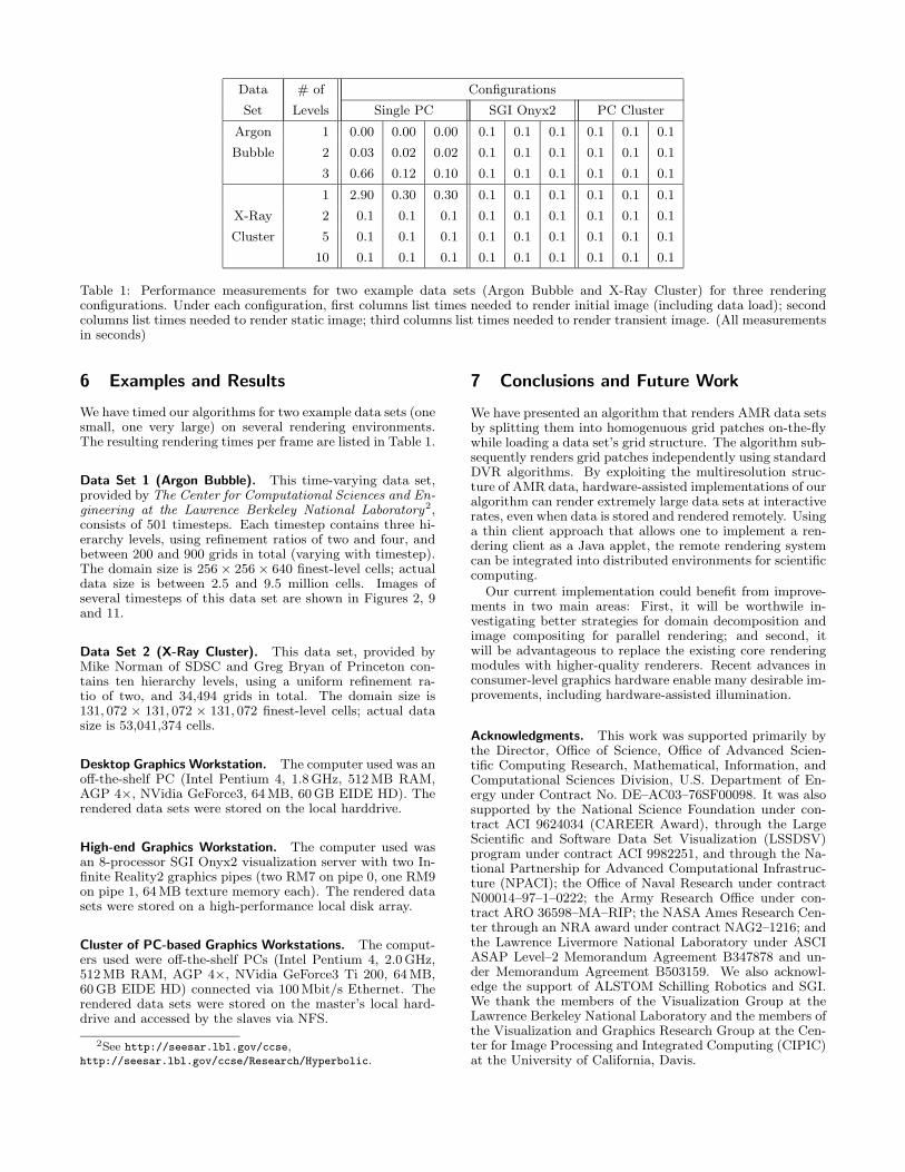
Table 1: Performance measurements for two example data sets (Argon Bubble and X-Ray Cluster) for three renderingconfigurations. Under each configuration, first columns list times needed to render initial image (including data load); secondcolumns list times needed to render static image; third columns list times needed to render transient image. (All measurementsin seconds)

6 Examples and Results

We have timed our algorithms for two example data sets (onesmall, one very large) on several rendering environments.The resulting rendering times per frame are listed in Table 1.

Data Set 1 (Argon Bubble). This time-varying data set,provided by The Center for Computational Sciences and En-gineering at the Lawrence Berkeley National Laboratory2,consists of 501 timesteps. Each timestep contains three hi-erarchy levels, using refinement ratios of two and four, andbetween 200 and 900 grids in total (varying with timestep).The domain size is 256 × 256 × 640 finest-level cells; actualdata size is between 2.5 and 9.5 million cells. Images ofseveral timesteps of this data set are shown in Figures 2, 9and 11.

Data Set 2 (X-Ray Cluster). This data set, provided byMike Norman of SDSC and Greg Bryan of Princeton con-tains ten hierarchy levels, using a uniform refinement ra-tio of two, and 34,494 grids in total. The domain size is131, 072 × 131, 072 × 131, 072 finest-level cells; actual datasize is 53,041,374 cells.

Desktop Graphics Workstation. The computer used was anoff-the-shelf PC (Intel Pentium 4, 1.8 GHz, 512 MB RAM,AGP 4×, NVidia GeForce3, 64 MB, 60 GB EIDE HD). Therendered data sets were stored on the local harddrive.

High-end Graphics Workstation. The computer used wasan 8-processor SGI Onyx2 visualization server with two In-finite Reality2 graphics pipes (two RM7 on pipe 0, one RM9on pipe 1, 64 MB texture memory each). The rendered datasets were stored on a high-performance local disk array.

Cluster of PC-based Graphics Workstations. The comput-ers used were off-the-shelf PCs (Intel Pentium 4, 2.0 GHz,512 MB RAM, AGP 4×, NVidia GeForce3 Ti 200, 64 MB,60 GB EIDE HD) connected via 100 Mbit/s Ethernet. Therendered data sets were stored on the master’s local hard-drive and accessed by the slaves via NFS.

2See http://seesar.lbl.gov/ccse,http://seesar.lbl.gov/ccse/Research/Hyperbolic.

7 Conclusions and Future Work

We have presented an algorithm that renders AMR data setsby splitting them into homogenuous grid patches on-the-flywhile loading a data set’s grid structure. The algorithm sub-sequently renders grid patches independently using standardDVR algorithms. By exploiting the multiresolution struc-ture of AMR data, hardware-assisted implementations of ouralgorithm can render extremely large data sets at interactiverates, even when data is stored and rendered remotely. Usinga thin client approach that allows one to implement a ren-dering client as a Java applet, the remote rendering systemcan be integrated into distributed environments for scientificcomputing.

Our current implementation could benefit from improve-ments in two main areas: First, it will be worthwile in-vestigating better strategies for domain decomposition andimage compositing for parallel rendering; and second, itwill be advantageous to replace the existing core renderingmodules with higher-quality renderers. Recent advances inconsumer-level graphics hardware enable many desirable im-provements, including hardware-assisted illumination.

Acknowledgments. This work was supported primarily bythe Director, Office of Science, Office of Advanced Scien-tific Computing Research, Mathematical, Information, andComputational Sciences Division, U.S. Department of En-ergy under Contract No. DE–AC03–76SF00098. It was alsosupported by the National Science Foundation under con-tract ACI 9624034 (CAREER Award), through the LargeScientific and Software Data Set Visualization (LSSDSV)program under contract ACI 9982251, and through the Na-tional Partnership for Advanced Computational Infrastruc-ture (NPACI); the Office of Naval Research under contractN00014–97–1–0222; the Army Research Office under con-tract ARO 36598–MA–RIP; the NASA Ames Research Cen-ter through an NRA award under contract NAG2–1216; andthe Lawrence Livermore National Laboratory under ASCIASAP Level–2 Memorandum Agreement B347878 and un-der Memorandum Agreement B503159. We also acknowl-edge the support of ALSTOM Schilling Robotics and SGI.We thank the members of the Visualization Group at theLawrence Berkeley National Laboratory and the members ofthe Visualization and Graphics Research Group at the Cen-ter for Image Processing and Integrated Computing (CIPIC)at the University of California, Davis.

References

[1] Berger, M. J., and Oliger, J., Adaptive Mesh Refinementfor Hyperbolic Partial Differential Equations, Journal ofComputational Physics 53 (1984), pp. 482–512

[2] Berger, M. J., and Colella, P., Local Adaptive Mesh Re-finement for Shock Hydrodynamics, Journal of Compu-tational Physics 82 (1989), pp. 64–84

[3] Pember, R. B., Bell, J. B., Colella, P., Crutchfield,W. Y., and Welcome, M. L., An Adaptive CartesianGrid Method for Unsteady Compressible Flow in Ir-regular Regions, Journal of Computational Physics 120(1995), pp. 278–304

[4] Aftosmis, M. J., Berger, M. J., and Melton, J. E., Adap-tive Cartesian Mesh Generation, in: Thompson, J. F.,Soni, B. K., and Weatherill, N. P., eds., Handbook ofGrid Generation (1999), CRC Press, Boca Raton,Florida, pp. 22-1–22-26

[5] Drebin, R. A., Carpenter, L. and Hanrahan, P., Vol-ume Rendering, Computer Graphics 22(4) (Proc. SIG-GRAPH ’88) (1988), pp. 65–74

[6] Levoy, M., Display of Surfaces from Volume Data, IEEEComputer Graphics and Applications 8(3) (1988),pp. 29–37

[7] Max, N. L., Hanrahan, P. and Crawfis, R., Area andVolume Coherence for Efficient Visualization of 3DScalar Functions, Computer Graphics 24(5) (Proc. SIG-GRAPH ’90) (1990), pp. 27–33

[8] Lacroute, P., and Levoy, M., Fast Volume Render-ing Using a Shear-Warp Factorization of the ViewingTransformation, Computer Graphics 28(4) (Proc. SIG-GRAPH ‘94) (1994), pp. 451–458

[9] Westover, L., Footprint Evaluation for Volume Render-ing, Computer Graphics 24(4) (Proc. SIGGRAPH ’90)(1990), pp. 367–376

[10] Cabral, B., Cam, N. and Foran, J., Accelerated Vol-ume Rendering and Tomographic Reconstruction UsingTexture Mapping Hardware, Proc. 1994 ACM Sympo-sium on Volume Visualization (1994), ACM Press, NewYork, New York, pp. 91–98

[11] Van Gelder, A. and Kim, K., Direct Volume Ren-dering with Shading via Three-Dimensional Textures,Proc. 1996 Symposium on Volume Visualization (1996),IEEE Computer Society Press, Los Alamitos, Califor-nia, pp. 23–ff.

[12] Rezk-Salama, C., Engel, K., Bauer, M., Greiner,G. and Ertl, T., Interactive Volume Renderingon Standard PC Graphics Hardware Using Multi-Textures and Multi-Stage Rasterization, Proc. 2000SIGGRAPH/EUROGRAPHICS Workshop on Graph-ics Hardware (2000), held in Interlaken, Switzerland,ACM Press, New York, New York, pp. 109–118

[13] Shirley, P. and Tuchman, A., A Polygonal Approxi-mation to Direct Scalar Volume Rendering, ComputerGraphics 24(5) (San Diego Workshop on Volume Visu-alization) (1990), pp. 63–70

[14] Yagel, R., Reed, D. M., Law, A., Shih, P.-W. andShareef, N., Hardware Assisted Volume Rendering ofUnstructured Grids by Incremental Slicing, Proc. 1996Symposium on Volume Visualization (1996), IEEEComputer Society Press, Los Alamitos, California,pp. 55–ff.

[15] Weber, G. H., Kreylos, O., Ligocki, T. J., Shalf, J. M.,Hagen, H., Hamann, B., Joy, K. I. and Ma, K.-L., High-Quality Volume Rendering of Adaptive Mesh Refine-ment Data, in: Ertl. T., Girod, B., Greiner, G., Nie-mann, H. and Seidel, H.-P., eds., Vision, Modeling andVisualization 2001 (2001), IOS Press, Amsterdam, TheNetherlands, pp. 121–128

[16] Porter, T. and Duff, T., Compositing Digital Im-ages, Computer Graphics 18(3) (Proc. SIGGRAPH ‘84)(1984), pp. 253–259

[17] Samet, H., The Design and Analysis of Spatial DataStructures (1999), Addison-Wesley Publishing Com-pany, Inc., Reading, Massachusetts

[18] LaMar, E. C., Hamann, B. and Joy, K. I., Multiresolu-tion Techniques for Interactive Texture-Based VolumeVisualization, in: Ebert, D., Gross, M. H. and Hamann,B., eds., Proc. Visualization ’99 (1999), IEEE SocietyPress, Los Alamitos, California, pp. 355–361, 543

[19] Ma, K.-L., Painter, J. S., Hansen, C. D. and Krogh,M. F., A Data Distributed, Parallel Algorithm for Ray-Traced Volume Rendering, Proc. 1993 Symposium onParallel Rendering (1993), ACM Press, New York, NewYork, pp. 15–22

[20] Bethel, E. W., et. al., Using High-Speed WANs and Net-work Data Caches to Enable Remote and DistributedVisualization, in: Proc. IEEE SC2000, The SCxy Con-ference Series, Dallas, Texas, November 2000