Copyright 2004 Society of Photo-Optical Instrumentation Engineers. This paper will be published in Remote Sensing of Clouds and the Atmosphere, Proceedings of SPIE Vol. 5235 and is made available as an electronic preprint with permission of SPIE. One print or electronic copy may be made for personal use only. Systematic or multiple reproduction, distribution to multiple locations via electronic or other means, duplication of any material in this paper for a fee or for commercial purposes, or modification of the content of the paper are prohibited.

Remote Detection of Methane by Infrared Spectrometry for Airborne Pipeline Surveillance: First Results of Ground-Based Measurements

Roland Harig*a, Gerhard Matza, Peter Ruscha, Jörn-Hinnrich Gerharda, Klaus Schäferb, Carsten Jahnb, Peter Schwenglerc, Andreas Beild

aTechnische Universität Hamburg-Harburg, D-21079 Hamburg bIMK-IFU, Forschungszentrum Karlsruhe, Kreuzeckbahnstr. 19, D-82467 Garmisch-Partenkirchen

cRuhrgas Aktiengesellschaft, Huttropstraße 60, D-45138 Essen dBruker Daltonik GmbH, Permoserstr. 15, D-04318 Leipzig

ABSTRACT The total length of natural gas pipelines in Germany exceeds 350,000 km. Currently, inspections are performed using hand-held sensors such as flame ionization detectors. Moreover, transmission pipelines are inspected visually from helicopters. In this work, remote detection of methane by passive Fourier-transform infrared (FTIR) spectrometry for pipeline surveillance is investigated. The study focuses on fast measurements in order to enable methane detection from a helicopter during regular inspection flights. Two remote sensing systems are used for the detection of methane: a scanning infrared gas imaging system (SIGIS), which was originally developed for the visualization of pollutant clouds, and a new compact passive scanning remote sensing system. In order to achieve a high spectral rate, which is required due to the movement of the helicopter, measurements are performed at low spectral resolutions. This results in overlapping signatures of methane and other constituents of the atmosphere in the measured spectrum. The spectra are analyzed by a detection algorithm, which includes simultaneous least squares fitting of reference spectra of methane and other atmospheric species. The results of field measurements show that passive remote sensing by FTIR spectrometry is a feasible method for the remote detection of methane. Keywords: methane; remote sensing; FTIR; passive; imaging spectrometry; scanning imaging FTIR spectrometer; pipeline surveillance; passive infrared spectrometry 1. INTRODUCTION Transmission pipelines for natural gas have to be monitored regularly. Due to the length of the pipeline system and the inaccessibility of some areas under which pipelines are buried, inspections are performed using helicopters. Currently, these inspections are performed visually. However, for the detection of small leaks, ground-based systems such as flame ionization detectors are used. The goal of various current research activities are remote sensing systems for the detection of leaks from a helicopter. In this work, remote detection of methane by Fourier transform infrared spectrometry for pipeline surveillance is investigated. The study focuses on fast measurements in order to enable methane detection during regular inspection flights. The minimum time required for the measurement of a spectrum (i.e. the time for the measurement of one interferogram) is inversely proportional to the spectral resolution, i.e. the width of the instrument line shape ∆σ. Thus, the possibility of performing measurements with low spectral resolutions is investigated. 2. PASSIVE REMOTE SENSING OF METHANE BY INFRARED SPECTROMETRY 2.1 Radiative Transfer Model Passive remote sensing of gas clouds in the lower atmosphere is based on the analysis of radiation absorbed and emitted by the molecules of the clouds. Figure 1 illustrates the measurement setup for airborne pipeline surveillance. In order to

* harig@tuhh.de; http://www.et1.tu-harburg.de/ftir ; Technische Universität Hamburg-Harburg, Arbeitsbereich Messtechnik, Harburger Schlossstr. 20, D-21079 Hamburg, Germany

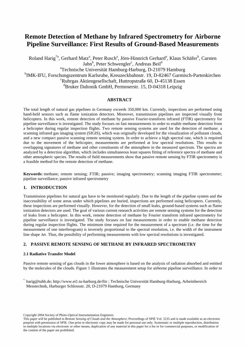
describe the characteristics of spectra measured by a passive infrared spectrometer a model in which the atmosphere is divided into plane-parallel homogeneous layers along the optical path may be used1,2. In most cases a model with three layers is sufficient to describe the basic characteristics of the spectra (Figure 1). Radiation from the background (layer 3) propagates through the vapor cloud (layer 2) and the atmosphere between the cloud and the spectrometer (layer 1). The cloud and atmospheric layers are considered homogeneous with regard to all physical and chemical properties. The radiation containing the signatures of all layers is measured by the spectrometer.

1

2

3

T1,τ1

Spectrometer

T3, ε Ground surface

T2τ2

Lamb

Methane

Lsky

Atmosphere(approx. 100 m)

Figure 1: Radiative transfer model.

In this model the spectral radiance at the entrance aperture of the spectrometer L1 is

[ ]32221111 )1()1( LBBL ττττ +−+−= , (1) where τi is the transmittance of layer i, Bi is the spectral radiance of a blackbody at the temperature of layer i, Ti. L3 is the radiance that enters the layer of the cloud from the background. The quantities in Equation (1) are frequency-dependent. The radiation entering the cloud L3 contains radiation emitted by the surface and reflected radiation1:

)()()(),(2

3 bgsdowns TBdLFaL Ω+Ω′Ω′−Ω′−Ω= ∫ επ

. (2)

Here, a is the surface albedo, Ωs is the solid angle subtended by the aperture of the spectrometer. F(Ωs,-Ω) is the surface biconical reflectance function for incident solid angle -Ω and emergent solid angle Ωs. ε(Ωs) is the directional surface emittance, and B(Tbg) is the radiance emitted by a blackbody at temperature Tbg. The radiation incident on the background Ldown contains ambient radiation (Lam) and radiation from the sky (Lsky). The dependence on frequency is left implicit again. If the temperatures of the layers 1 and 2 are equal, Equation (1) can be simplified: ( )132111 BLBL −+= ττ (3) 2.2 Brightness Temperature The brightness temperature Tbr is defined by the Planck function: ( ) )()(, σσσ LTB br = , (4)

where L(σ) is the spectral radiance and σ is the frequency (wavenumber, expressed in cm-1). It is calculated by solving Eq. (4) for Tbr

kLhc

hcTbr

⎥⎥⎦

⎤

⎢⎢⎣

⎡+

=

1)(

2ln

)(32

σσ

σσ (5)

[h: Planck’s constant, c: speed of light, k: Boltzmann’s constant]. The emittance ε(σ) of many surfaces is high and almost constant in the range 650 – 1500 cm-1. Thus, the emission spectrum of these materials has a high degree of similarity to the spectrum of a blackbody and the spectrum of the brightness temperature Tbr(σ) of these surfaces is almost constant. This makes the brightness temperature spectrum well suited for direct analysis without measurement of a background spectrum3. 2.3 Spectral Resolution and Detection Limit The choice of the spectral resolution is a compromise between higher signal-to-noise ratios and higher maximum spectral rates for low resolution spectra and more spectral information if high-resolution spectra are measured4,5,6. Since measurements will be performed from a helicopter, high spectral rates are required. Moreover, low limits of detection are essential. On the other hand, the absorption bands of methane and other trace gases of the atmosphere (in particular water) overlap. In order to detect methane lines in the presence of these signatures, high spectral resolution is advantageous.

1280 1290 1300 1310 1320 1330288

289

290

1280 1290 1300 1310 1320 1330288

289

290

1280 1290 1300 1310 1320 1330288

289

290

1280 1290 1300 1310 1320 1330288

289

290

clMethane= 500 ppm m (layer 2) clMethane= 0 ppm m (layer 2)

∆σ = 1 cm-1

∆σ = 9 cm-1

Wavenumber (cm-1)

Wavenumber (cm-1)

Brig

htne

ss T

empe

ratu

re (K

)B

right

ness

Tem

pera

ture

(K)

∆σ = 0.6 cm-1

∆σ = 4 cm-1

Wavenumber (cm-1)

Wavenumber (cm-1)

Brig

htne

ss T

empe

ratu

re (K

)B

right

ness

Tem

pera

ture

(K)

Figure 2: Simulated spectra of 500 ppm m methane (layer 2, solid line) and spectra without methane in layer 2 (dashed line)with different spectral resolutions.

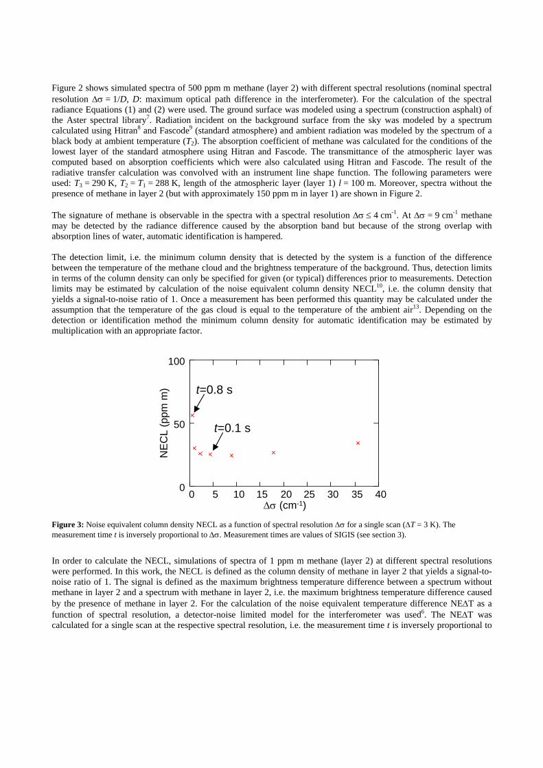
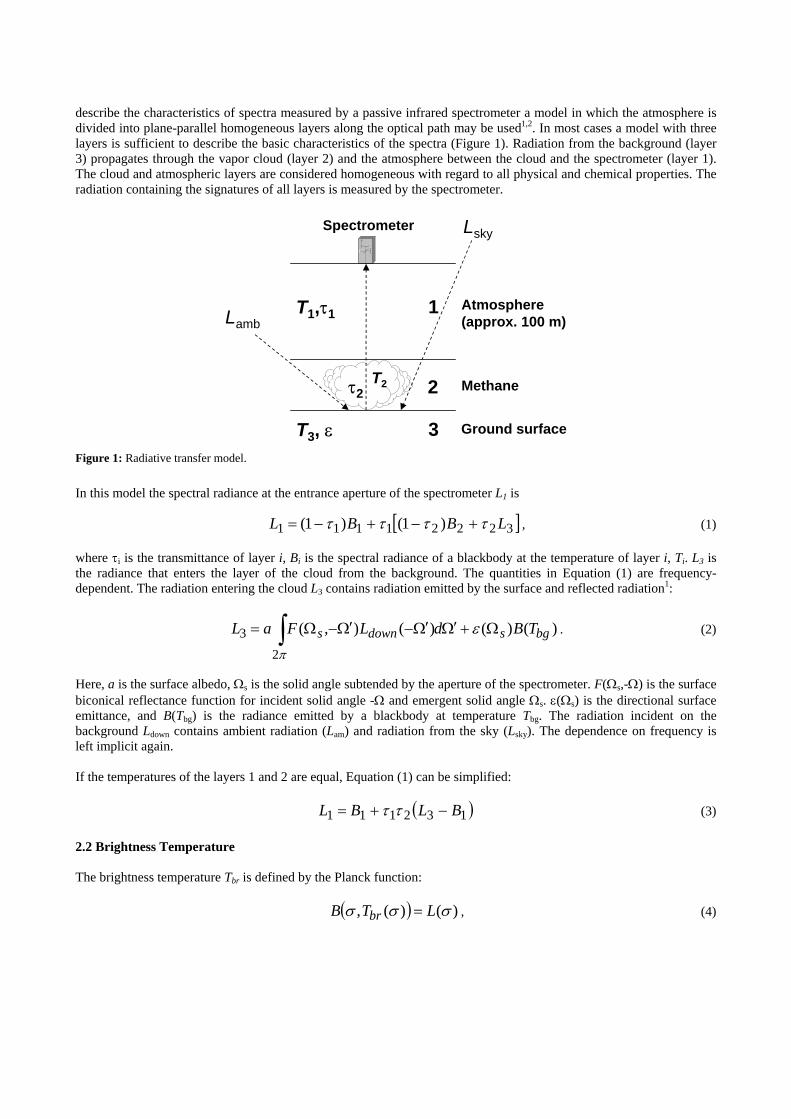
Figure 2 shows simulated spectra of 500 ppm m methane (layer 2) with different spectral resolutions (nominal spectral resolution ∆σ = 1/D, D: maximum optical path difference in the interferometer). For the calculation of the spectral radiance Equations (1) and (2) were used. The ground surface was modeled using a spectrum (construction asphalt) of the Aster spectral library7. Radiation incident on the background surface from the sky was modeled by a spectrum calculated using Hitran8 and Fascode9 (standard atmosphere) and ambient radiation was modeled by the spectrum of a black body at ambient temperature (T2). The absorption coefficient of methane was calculated for the conditions of the lowest layer of the standard atmosphere using Hitran and Fascode. The transmittance of the atmospheric layer was computed based on absorption coefficients which were also calculated using Hitran and Fascode. The result of the radiative transfer calculation was convolved with an instrument line shape function. The following parameters were used: T3 = 290 K, T2 = T1 = 288 K, length of the atmospheric layer (layer 1) l = 100 m. Moreover, spectra without the presence of methane in layer 2 (but with approximately 150 ppm m in layer 1) are shown in Figure 2. The signature of methane is observable in the spectra with a spectral resolution ∆σ ≤ 4 cm-1. At ∆σ = 9 cm-1 methane may be detected by the radiance difference caused by the absorption band but because of the strong overlap with absorption lines of water, automatic identification is hampered. The detection limit, i.e. the minimum column density that is detected by the system is a function of the difference between the temperature of the methane cloud and the brightness temperature of the background. Thus, detection limits in terms of the column density can only be specified for given (or typical) differences prior to measurements. Detection limits may be estimated by calculation of the noise equivalent column density NECL10, i.e. the column density that yields a signal-to-noise ratio of 1. Once a measurement has been performed this quantity may be calculated under the assumption that the temperature of the gas cloud is equal to the temperature of the ambient air13. Depending on the detection or identification method the minimum column density for automatic identification may be estimated by multiplication with an appropriate factor.

∆σ (cm-1)

NE

CL

(ppm

m)

0 5 10 15 20 25 30 35 400

50

100

t=0.8 s

t=0.1 s

Figure 3: Noise equivalent column density NECL as a function of spectral resolution ∆σ for a single scan (∆T = 3 K). The measurement time t is inversely proportional to ∆σ. Measurement times are values of SIGIS (see section 3).

In order to calculate the NECL, simulations of spectra of 1 ppm m methane (layer 2) at different spectral resolutions were performed. In this work, the NECL is defined as the column density of methane in layer 2 that yields a signal-to-noise ratio of 1. The signal is defined as the maximum brightness temperature difference between a spectrum without methane in layer 2 and a spectrum with methane in layer 2, i.e. the maximum brightness temperature difference caused by the presence of methane in layer 2. For the calculation of the noise equivalent temperature difference NE∆T as a function of spectral resolution, a detector-noise limited model for the interferometer was used6. The NE∆T was calculated for a single scan at the respective spectral resolution, i.e. the measurement time t is inversely proportional to

∆σ and the NE∆T is proportional to ∆σ-1/2. For the calculation a value of NE∆T = 30 mK at ∆σ = 4 cm-1 was used. The NECL was estimated by division of the column density of methane in layer 2 by the signal-to-noise ratio at this column density (valid approximation for high transmittance, i.e. e-x≈1-x). For the simulation of the spectra, the following parameters were used: background material: construction asphalt (Aster spectral library), T3 = 288 K, T2 = T1 = 285 K (Difference ∆T = 3 K), length of the atmospheric layer (layer 1) l = 100 m. Figure 3 shows the results for the NECL for a single scan of the interferometer as a function of spectral resolution. The lowest noise equivalent column densities are obtained at spectral resolutions in the range 2 - 9 cm-1. Due to the requirements of a high spectral rate and low NECL, low spectral resolutions (2 - 4 cm-1) were chosen for this work. 2.4 Detection and Visualization of Methane The detection method is based on the approximation of a measured spectrum with a linear combination of reference spectra. First, the spectrum of the brightness temperature Tbr(σ) is calculated. The spectrum is analyzed sequentially for a variable number of target compounds - which are contained in a spectral library - with different reference matrices. Each matrix contains spectral data of one target compound (here: methane), atmospheric gases (e.g. H2O), and it may contain the signatures of potential interferents. Moreover, it contains functions for the approximation of the baseline. The frequency dependence of the brightness temperature of the background and thermal effects inside the spectrometer11,12 may cause baseline shifts that exceed the signal of the target compound. The identification is performed in three steps. In the first step, the mean brightness temperature is subtracted and the signatures contained in the matrix are fitted to the resulting spectrum (Figure 4). In the next step, the contributions of all fitted signatures (i.e. interferents, atmospheric species, and baseline) except the signature of the target compound are subtracted from the measured spectrum (Figure 4).

1280 1290 1300 1310 13204

2

0

2

Wavenumber (cm-1)

∆T (K

)

Measurement Fit

1280 1290 1300 1310 13202

1.5

1

0.5

0

Wavenumber (cm-1)

∆T (K

)

Measurement(after subtraction) Reference

Figure 4: Analysis of a spectrum. Left: Measured brightness temperature spectrum and result of the least squares fitting procedure. Right: Measured spectrum after subtraction of the baseline and atmospheric signatures except methane and reference spectrum of methane.

In order to decide if the target compound is present, the coefficient of correlation between the corrected spectrum, i.e. the result of the subtraction, and a reference spectrum is calculated in a compound specific number of spectral windows. Moreover, the coefficient of correlation between the fitted spectrum and the measured spectrum is calculated. The signal-to-noise ratio is calculated by division of the maximum brightness temperature difference caused by the target compound (determined by the least squares fitting procedure) by the noise equivalent temperature difference of the spectrum. If all coefficients of correlation and the signal-to-noise ratio are greater than compound specific threshold values, the target compound is identified. This calculation is performed for three different column densities of the target compound. The reference spectra with different column densities are calculated by convolution of high-resolution transmittance spectra (e.g. calculated with absorption coefficients computed using Hitran/Fascode) with an instrument line shape function. The instrument line shape function is calculated by convolution of an ideal instrument line shape function (Fourier transform of the apodization function) and an inherent line shape function describing the effects of the finite étendue, aberrations etc. on the instrument line shape. Optionally, the difference between two spectra, a background spectrum and the last measured spectrum, can be analyzed in addition to the direct analysis of brightness

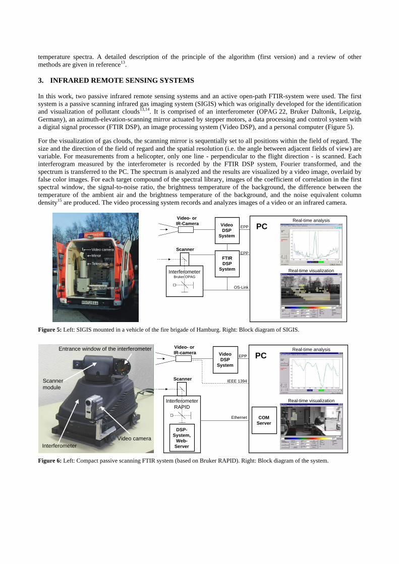
temperature spectra. A detailed description of the principle of the algorithm (first version) and a review of other methods are given in reference13. 3. INFRARED REMOTE SENSING SYSTEMS In this work, two passive infrared remote sensing systems and an active open-path FTIR-system were used. The first system is a passive scanning infrared gas imaging system (SIGIS) which was originally developed for the identification and visualization of pollutant clouds13,14. It is comprised of an interferometer (OPAG 22, Bruker Daltonik, Leipzig, Germany), an azimuth-elevation-scanning mirror actuated by stepper motors, a data processing and control system with a digital signal processor (FTIR DSP), an image processing system (Video DSP), and a personal computer (Figure 5). For the visualization of gas clouds, the scanning mirror is sequentially set to all positions within the field of regard. The size and the direction of the field of regard and the spatial resolution (i.e. the angle between adjacent fields of view) are variable. For measurements from a helicopter, only one line - perpendicular to the flight direction - is scanned. Each interferogram measured by the interferometer is recorded by the FTIR DSP system, Fourier transformed, and the spectrum is transferred to the PC. The spectrum is analyzed and the results are visualized by a video image, overlaid by false color images. For each target compound of the spectral library, images of the coefficient of correlation in the first spectral window, the signal-to-noise ratio, the brightness temperature of the background, the difference between the temperature of the ambient air and the brightness temperature of the background, and the noise equivalent column density15 are produced. The video processing system records and analyzes images of a video or an infrared camera.

Interferometer

Telescope

Mirror

Video camera

InterferometerBruker OPAG

Scanner

FTIRDSP

System

VideoDSP

System

Video- or IR-Camera

EPP

EPP

OS-Link

Real-time analysis

Real-time visualization

PC

Figure 5: Left: SIGIS mounted in a vehicle of the fire brigade of Hamburg. Right: Block diagram of SIGIS.

Video camera

Entrance window of the interferometer

Scannermodule

Interferometer

PC

InterferometerRAPID

Scanner

DSP-System,

Web-Server

VideoDSP

System

Video- or IR-camera

Ethernet COMServer

IEEE 1394

Real-time analysis

Real-time visualization

EPP

Figure 6: Left: Compact passive scanning FTIR system (based on Bruker RAPID). Right: Block diagram of the system.

The second passive scanning FTIR system is based on an interferometer with an azimuth-elevation-scanning system (Bruker RAPID). It has been equipped with an additional video system. The detection and visualization software described previously has been extended in order to record and analyze interferograms measured by this interferometer. At a spectral resolution of 3 cm-1 up to 32 spectra per second are recorded, analyzed and visualized in a video image (Figure 6). Design and performance parameters of the passive remote sensing systems are given in Table 1. Active open-path FTIR measurements were performed with a Kayser-Threde K 300 (Kayser-Threde, Munich, Germany) spectrometer16.

Table 1: Specifications of the passive scanning FTIR systems.

SIGIS RAPID-based system

Interferometer Bruker OPAG Bruker RAPID

Spectral range 680 – 1500 cm-1 (600 - 6000 cm-1 max.)

680 – 1500 cm-1 (600 - 6000 cm-1 max.)

Maximum spectral resolution (nominal, ∆σ = 1/D)

0.6 cm-1 (D = 1.8 cm)

1.1 cm-1 (D = 0.9 cm)

Spectral resolution (this work) 4 cm-1 2 cm-1 and 3 cm-1

Field of view 7.5 mrad 30 mrad

Field of regard 285°×80° 360°×60°

Maximum spectral rate 7 spectra/s (∆σ = 4 cm-1) 32 spectra/s (∆σ = 3 cm-1, single sided interferograms)

NE∆T (triangular apodization, 1000 cm-1)

20 mK (∆σ = 4 cm-1, t = 0.1 s) 40 mK (∆σ = 3 cm-1, t = 0.05 s, 16 spectra/s)

4. FIELD EXPERIMENTS In order to simulate a leak in a pipeline, methane was released approximately 1 m below the ground. Measurements were performed from the roof of a building at a distance of approximately 100 m. During the measurements weak winds prevailed. Figure 7 shows the location of the release of methane from the position of the remote sensing system. For each measurement, a field of regard consisting of 30 × 20 directions was scanned. The results are visualized in false color images as described above. In each direction of the scanning mirror, one interferogram was measured. For the detection of methane, the spectra were analyzed in the spectral range 1280 - 1320 cm-1. The radiation source, which is used for the active open-path measurements (not for the passive measurements) is also shown in Figure 7.

Globar for activeopen-path measurements

Release of Methane

Active open-path FTIR-system (not shown, 92 m from Globar)

Figure 7: Photograph of the location of the release of methane taken from the position of the remote sensing system.

Figure 8 shows results of measurements at a release rate of 0.5 m3/h. The analysis yields a high coefficient of correlation (1290 - 1315 cm-1) in many directions within the field of regard. However, in combination with the signal-to-noise ratio, the position of the release of methane is identifiable and methane is identified automatically by the identification algorithm.

0 1Coefficient of correlation R

0 8.5Signal-to-noise ratio

Figure 8: Left: Video image overlaid by a false color image of the coefficient of correlation. Right: Video image overlaid by a false color image of the signal-to-noise ratio. The release rate of methane was 0.14 L/s (0.5 m3/h).

-0.2 1Coefficient of correlation R

0 7.3Signal-to-noise ratio

Figure 9: Left: Video image overlaid by a false color image of the coefficient of correlation. Right: Video image overlaid by a false color image of the signal-to-noise ratio. The release rate of methane was 0.014 L/s (0.05 m3/h).

Figure 9 shows results of measurements at a release rate of 0.05 m3/h. Around the position of the release of methane, the coefficient of correlation and the signal to noise ratio increase slightly. Figure 10 shows results of active open-path measurements. The length of the absorption path was 92 m. During both releases the path-averaged concentration of methane was higher than the concentration of methane in the ambient air.

X Path-averaged concentration of MethaneMean concentration of MethaneMean concentration of Methane in ambient air

0.00

0.50

1.00

1.50

2.00

2.50

3.00

14:45 15:15 15:45 16:15 16:45 17:15 17:45Time (hh:mm)

c CH

4 (pp

m)

15:00 h - 15:30 hRelease of 0.14 L/s

16:52 h - 17:20 hRelease of 0.014 L/s

Figure 10: Results of active open-path measurements.

In another experiment, methane was released above the ground. Measurements were performed from a building at a distance of approximately 100 m. Figure 11 shows results of measurements at a release rate of 0.14 L/s (0.5 m3/h). The analysis yields a high coefficient of correlation around the position of the release of methane. In the image of the signal-to-noise ratio the location of the release of methane is also identifiable.

0 1Coefficient of correlation R

0 30Signal-to-noise ratio

Figure 11: Left: False color image of the coefficient of correlation. Right: False color image of the signal-to-noise ratio. The release rate of methane was 0.14 L/s (0.5 m3/h).

Figure 12 shows results of measurements at a release rate 0.4 L/s (1.3 m3/h, released 1 m below the ground). The methane cloud is clearly observable in the image of the coefficient of correlation and in the image of the signal-to-noise ratio.

0.8 1Coefficient of correlation R

0 86Signal-to-noise ratio

Figure 12: Left: False color image of the coefficient of correlation. Right: False color image of the signal-to-noise ratio. The release rate of methane was 0.4 L/s (1.3 m3/h).

Figure 13 shows results of measurements with the new scanning remote sensing system (∆σ = 2 cm-1). The release rate of methane was 0.4 L/s. The lower spatial resolution in comparison with the images obtained with the system with telescope is due to the larger field of view of this system. The methane cloud is observable in the image of the coefficient of correlation and in the image of the signal-to-noise ratio.

0 1Coefficient of correlation R

0 29Signal-to-noise ratio

Figure 13: Results of measurements with the new scanning remote sensing system. Left: False color image of the coefficient of correlation. Right: False color image of the signal-to-noise ratio. The release rate of methane was 0.4 L/s (1.3 m3/h).

5. CONCLUSIONS Methane was detected at release rates in the range 0.05 - 1.3 m3/h. The superposition of a video image by false color images of the results of the identification algorithm allows the localization of the source of methane. The compact scanning remote sensing system based on the system RAPID allows the measurement, analysis, and visualization of up to 32 spectra per second at a spectral resolution of 3 cm-1. The results of the field measurements show that passive remote sensing by FTIR spectrometry is a feasible method for the remote detection of methane. However, although not shown in this work, the probability of detection is strongly dependent on the weather conditions, in particular the wind and the difference between the temperature of the methane cloud and the brightness temperature of the background. Thus, additional experiments under various weather conditions have to be performed in order to evaluate detection capabilities under the respective conditions. 6. ACKNOWLEDGEMENTS The authors thank the Zentralstelle für Zivilschutz des Bundesverwaltungsamtes for providing the interferometer Bruker OPAG 22. 7. REFERENCES 1. Beer, R.: “Remote Sensing by Fourier Transform Spectrometry,” (Wiley, New York 1992). 2. Flanigan, D. F.: “Prediction of the limits of detection of hazardous vapors by passive infrared with the use of

Modtran,“ Applied Optics 35, 6090-6098 (1996). 3. Beil, A., Daum, R., Matz, G., Harig, R.: “Remote sensing of atmospheric pollution by passive FTIR spectrometry“

in Spectroscopic Atmospheric Environmental Monitoring Techniques, Klaus Schäfer, Editor, Proceedings of SPIE Vol. 3493, 32-43 (1998).

4. Flanigan, D. F.: “Vapor-detection sensitivity as a function of spectral resolution for a single lorentzian band,“ Applied Optics 34, 2636-2639 (1995).

5. Griffiths, P. R.: “Fourier Transform Infrared Spectrometry at Low Resolution: How Low Can You Go?,” Proc. SPIE 2089, 2-8 (1993).

6. Harig, R.: “Passive remote sensing of pollutant clouds by FTIR spectrometry: Signal-to-noise ratio as a function of spectral resolution,” in preparation.

7. http://speclib.jpl.nasa.gov 8. Rothman, L., Rinsland, C., Goldman, A., Massie, S., Edwards, D., Flaud, J., Perrin, A., Camy-Peyret, C., Dana,

V., Mandin, J., Schroeder, J., McCann, A., Gamache, R., Wattson, R., Yoshino, K., Chance, K., Jucks, K., Brown, L., Nemtchinov, V., Varanasi, P.: “The HITRAN Molecular Spectroscopic Database and HAWKS (HITRAN Atmospheric Workstation): 1996 Edition,” Journal of Quantitative Spectroscopy and Radiative Transfer 60, 665-710 (1998).

9. Smith, H.J.P., Dube, D.J, Gardner, M.E., Clough, S.A., Kneizys, F.X., Rothman, L.S.: “FASCODE- Fast Atmospheric Signature Code (Spectral Transmittance and Radiance),“ Air Force Geophysics Laboratory Technical Report AFGL-TR-78-0081, Hanscom AFB, MA (1978).

10. Flanigan, D. F.: “Detection of organic vapors with active and passive sensors: a comparison,“ Applied Optics 25, 4253-4260 (1986).

11. Combs, R. J.: “Thermal Stability Evaluation for Passive FTIR Spectrometry,“ Field Analytical Chemistry and Technology 3, 81–94 (1999).

12. Thériault, J.-M.: “Modeling the responsivity and self-emission of a double-beam Fourier-transform infrared interferometer”, Applied Optics 38, 505-515 (1999).

13. Harig, R., Matz, G.: “Toxic Cloud Imaging by Infrared Spectrometry: A Scanning FTIR System for Identification and Visualization,“ Field Analytical Chemistry and Technology 5 (1-2), 75-90 (2001).

14. Harig, R., Matz, G., Rusch, P.: “Scanning Infrared Remote Sensing System for Identification, Visualization, and Quantification of Airborne Pollutants“ in Instrumentation for Air Pollution and Global Atmospheric Monitoring, James O. Jensen, Robert L. Spellicy, Editors, Proc. SPIE 4574, 83-94 (2002).

15. Flanigan, D. F.: “Detection of organic vapors with active and passive sensors: a comparison,“ Applied Optics 25, 4253-4260 (1986).

16. Haus, R., Schäfer, K., Bautzer, W., Heland, J., Mosebach, H., Bittner, H., Eisenmann, T.: “Mobile FTIS-Monitoring of Air Pollution”, Applied Optics 33, 5682-5689 (1994).