remote ae monitoring of fatigue crack growth in … · remote ae monitoring of fatigue crack growth...
TRANSCRIPT

Remote AE Monitoring of Fatigue Crack Growth
in Complex Aircraft Structures
Milan CHLADA 1, Zdenek PREVOROVSKY
2
NDT Laboratory, Institute of Thermomechanics AS CR, v.v.i.,
Phone: +420 266 053 144, Fax: +420 286 584 695;
E-mail: 1 [email protected],
Abstract
Recently proposed AE source location method using so-called signal arrival time profiles and artificial neural
networks (ANN) was applied to growing defect monitoring during long-term fatigue test of aircraft structures.
The main goal of AE monitoring was to detect the growth of small cracks and to test the new AE source location
methodology as a part of Structural Health Monitoring system. The remote long distance on-line monitoring of
dangerous crack growth in critical aircraft structure parts was tested. The paper illustrates localization of large
amount of AE events, mostly of unknown or unconfirmed source origin. All finally revealed cracks were
predicted by AE before they became visible.
Keywords: Acoustic emission, source location, neural networks, arrival time profiles.
1. Introduction
Failures due to fracture of stressed mechanical structures, e.g., aircrafts, building units or
pressure vessels, can have major negative consequences, including serious injury or loss of
life, environmental damage, and substantial economic loss. Fatigue is one of the primary
reasons for the failure of structural components. The prediction of fatigue properties of
structures and avoiding material defect were recognized as engineering problems in the early
decades of the 20th century. The fatigue crack growth prediction models are fracture
mechanics based models that have been developed to support the damage tolerance concepts
in metallic structures. During the last decades, numerous methods have been published on
fatigue life and fatigue crack growth prediction under constant and variable amplitude
loading. Nevertheless, such approaches are usually applied off-line, i.e., during technical
inspections, which may not be able to disclose some critical defects hidden in
non-dismountable structure parts.
In principle, the acoustic emission (AE) represents one of NDT methods for the detection and
identification of growing material defects [1], so that this method is suitable for on-line
monitoring of potentially dangerous fatigue cracks in critical parts of technical structures.
Computational power of contemporary digital signal processors and the possibilities of
remote data transfer like the Internet and local Wi-Fi nets allow to design simple and
sufficiently fast on-line pre-warning systems. The practical part of this paper shows the
selected pictures illustrating the typical results of remotely controlled measurement of AE
during fatigue loading of riveted aircraft wing flange.
AE monitoring is widely applied in non-destructive testing of relatively simple structures up
to now, since the standard AE signal processing algorithms as AE localization or recognition
are not suitable for complex structure shapes and anisotropic materials. Hence, new
approaches to AE source location and classification are needed. As elements of artificial
intelligence systems, artificial neural networks (ANN) represent such suitable means and have
broad practical applications.
30th European Conference on Acoustic Emission Testing & 7th International Conference on Acoustic Emission University of Granada, 12-15 September 2012
www.ndt.net/EWGAE-ICAE2012/

Good knowledge of AE source location is the basic requirement for further damage
mechanism characterization. AE source coordinates are mostly determined by common
triangulation algorithm based on arrival time differences of AE signals recorded by several
transducers [2]. Analytical formulas are known for isotropic plates. However, there are many
practical situations in which the triangulation algorithm fails, especially if the more complex
structure is tested. Procedures based on ANN are used in such cases as an alternative
approach to triangulation algorithm. Unlike the classical methods, the ANN-based location
procedures have two important advantages: they are suitable for AE source location in highly
anisotropic media, and elastic wave velocity is not a necessary input parameter of the
algorithms [3, 4, 5].
2. Arrival time profile (ATP)
Contrary to the computational power of ANN's, their application possibility is strongly
restricted due to several reasons. The first problem is collection of sufficiently extensive
training and testing data sets, which may be too much time consuming, expensive or even
impossible in many cases. The most important reason is the non-portability of particular
trained network to any other configuration. ANN should be learned and applied on exactly the
same problem, i.e., on the same input-output parameter space. To solve both aspects for AE
source localization, new approach was recently introduced [6]. This innovative ANN-based
AE signal source location method uses new way of signal arrival time evaluation called signal
arrival time profiles, independently on the material and scale changes. Under some non-
restrictive conditions, such approach provides the ANN training on numerical models (i.e.,
without experimental errors) and allows the application of learned ANN on real structures of
various scales and materials.
The new way of signal arrival time treatment is inspired by the preliminary expert analysis of
AE source location. The whole monitored structure is separated into several zones according
to first arrival signal to each sensor. In this way, the AE source can be roughly localized using
the information which sensor is the nearest one. To describe the signal detection chronology
more precisely, so-called arrival time profiles were proposed. Let us suppose hypothetical
configuration of several AE sensors S1,...,SN placed on given material, detecting elastic waves
emitted by AE sources in various locations. Signal propagation time from the source to sensor
i is denoted Ti (arrival time period). Then, the arrival time profile (ATP) is a vector
of numbers pi defined as follows:
(1)
As no AE analyzer can measure arrival time periods Ti before the precise AE source location
is performed, the basic definition (1) is not usable. Only the AE signal arrival times ti are
available. Nevertheless, if we assume ts as the time of AE source initiation, it is easy to revise
the original formula, while Ti = ti - ts :
(2)
Computation of arrival time profiles is very similar to general data standardization. In a first
step, the mean value of arrival times is subtracted from each ti. Such data is then normalized
by the mean of its absolute values. If we assume the fastest elastic wave mode is propagating
in the structure by geometrically shortest ways, it is possible to compute ATP followed by
shortest distances from source to sensors. In case of simple homogeneous isotropic material
structures, where the direct linear connection between the two selected internal points is going
through the body, not outside of material, Euclidean source-sensor distance can be used. The
third dimension could be neglected for small material thickness as well. For more complex
structures represented for example by a digital photograph, the length of the real elastic wave
path through the material can be approximated by the shortest polygonal line, while the
connecting line segments between the nodes must come through the pixels representing the
body. Another algorithm for finding the shortest ways in parametrically described bodies is
the mathematical solution of geodetic curves.
2.1 Independence of ATP on wave velocity and scale changes
Let us denote di the distance between AE source and sensor i, and v the elastic wave velocity.
By substitution of relation Ti = di /v to (1) we obtain:
(3)
Arrival time profiles can be also calculated using the distances di, which enables the learning
of neural networks with numerically computed data from the distances measured on
proportional model of considered structure (i.e. without experimental errors) and, afterwards,
testing by processed real arrival times. The elastic wave velocity is cancelled out in eq. 3, so
the arrival time profiles are independent on elastic wave velocity. Analogical cancellation of
any common multiple of distances di proves the independence to structure scale changes.
3. Experiment - remotely controlled measurement
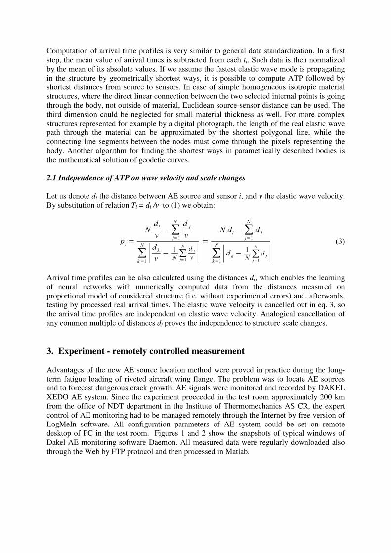
Advantages of the new AE source location method were proved in practice during the long-
term fatigue loading of riveted aircraft wing flange. The problem was to locate AE sources
and to forecast dangerous crack growth. AE signals were monitored and recorded by DAKEL
XEDO AE system. Since the experiment proceeded in the test room approximately 200 km
from the office of NDT department in the Institute of Thermomechanics AS CR, the expert
control of AE monitoring had to be managed remotely through the Internet by free version of
LogMeIn software. All configuration parameters of AE system could be set on remote
desktop of PC in the test room. Figures 1 and 2 show the snapshots of typical windows of
Dakel AE monitoring software Daemon. All measured data were regularly downloaded also
through the Web by FTP protocol and then processed in Matlab.
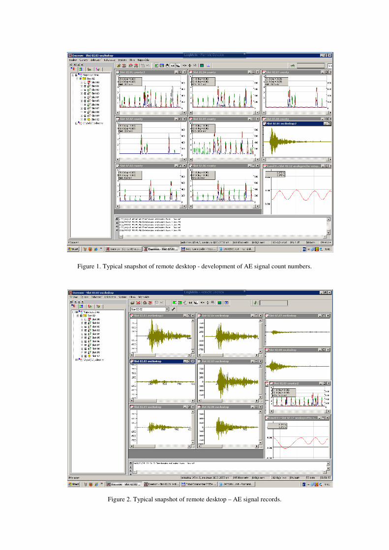
Figure 1. Typical snapshot of remote desktop - development of AE signal count numbers.
Figure 2. Typical snapshot of remote desktop – AE signal records.
For signal onset assessment, an "expert signal edge detection" algorithm of the elastic wave
arrival was applied [7]. Although the method is relatively precise, its accuracy is much lower
than the approximation error of neural networks, especially for longer distances from AE
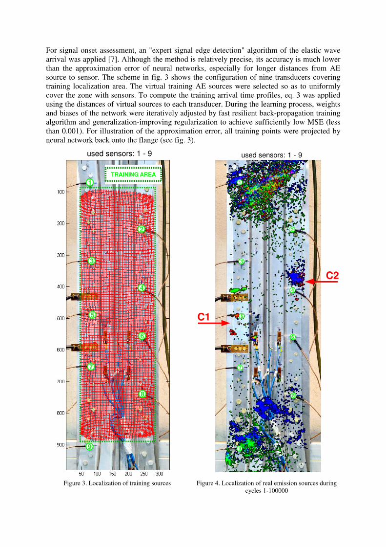
source to sensor. The scheme in fig. 3 shows the configuration of nine transducers covering
training localization area. The virtual training AE sources were selected so as to uniformly
cover the zone with sensors. To compute the training arrival time profiles, eq. 3 was applied
using the distances of virtual sources to each transducer. During the learning process, weights
and biases of the network were iteratively adjusted by fast resilient back-propagation training
algorithm and generalization-improving regularization to achieve sufficiently low MSE (less
than 0.001). For illustration of the approximation error, all training points were projected by
neural network back onto the flange (see fig. 3).
Figure 3. Localization of training sources Figure 4. Localization of real emission sources during
cycles 1-100000
C1
C2
1
2
3
4
5
6
7
8
9
used sensors: 1 - 9used sensors: 1 - 9
1
2
3
4
5
6
7
8
9
TRAINING AREA

Figure 5. Loading force (LF) envelope and its derivative during one typical "flight" period.
Trained neural networks were finally tested with real experimental data. The arrival times of
each signal were determined by the expert edge detection algorithm and eq. 2 was used to
compute the arrival time profiles as ANN inputs. The network outputs were coordinates of
estimated AE source locations illustrated as color clusters (figs. 4, 6, 7). Potential seriousness
of AE source is related with the loading force phase. Hence, the sources are distinguished by
different colors: AE signals recorded while derivative of loading force is negative or positive
(see fig. 5) have blue or green colors respectively, while the red color corresponds to
maximum loading peaks higher than 3.6V - see fig. 5. The brightness of colors is proportional
to the number of localized AE hits in respective pixels. In a case of different sources
overlapping, the additive color synthesis is applied.
4. Discussion of results
The main goal of AE monitoring was to detect the growth of small artificial crack (marked as
C1 in figs. 4, 6, 7) initiated at the rim of the rivet hole in central left part of the flange. Fig. 4
shows the localization of AE activity within the loading during the first part of experiment,
while data from all sensors were used. Precise observation by a microscope proved the growth
of crack C1, however the detected emission activity from corresponding coordinates was very
weak. One probable cause is overloading of measuring system by too frequent emission from
other parts of the flange. Localization inaccuracies are mostly related with experimental
errors, mostly caused by the improper signal onset determination. Due to the wave dispersion
and reflections, the signal waveform envelope undergoes substantial changes with distance
between the source and sensor. As to eliminate the highest errors, only the AE sources within
the zone around the sensor detecting first AE signal arrival were taken into account.
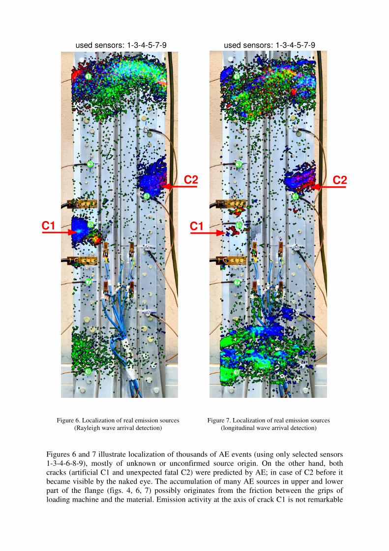
Figure 6. Localization of real emission sources
(Rayleigh wave arrival detection) Figure 7. Localization of real emission sources
(longitudinal wave arrival detection)
Figures 6 and 7 illustrate localization of thousands of AE events (using only selected sensors
1-3-4-6-8-9), mostly of unknown or unconfirmed source origin. On the other hand, both
cracks (artificial C1 and unexpected fatal C2) were predicted by AE; in case of C2 before it
became visible by the naked eye. The accumulation of many AE sources in upper and lower
part of the flange (figs. 4, 6, 7) possibly originates from the friction between the grips of
loading machine and the material. Emission activity at the axis of crack C1 is not remarkable
C1
C2
1
3
4
5
7
9
used sensors: 1-3-4-5-7-9
C1
C2
1
3
4
5
7
9
used sensors: 1-3-4-5-7-9

in fig.7. Probably due to small amplitude of signals that caused the arrival time detection error
for sensors at longer distances from the AE source. Conversely, the activity at the axis of the
future crack C2 is evident. The searching of origin of other AE sources did not succeed. There
was no visible damage that could clarify the inception of sources especially between the
sensors 7 and 9 (see the expressive green clusters in fig. 7).
The two pictures (figs. 6 and 7) differ by the version of applied arrival detection algorithm.
We can see remarkably different results using the method for longitudinal or Rayleigh wave.
The emission activity at the place of expected break resulting from artificially initiated crack
C1 was detected more likely by Rayleigh waves, while both methods predicted the
unexpected final brakeage at the axes of crack C2.
Acknowledgements The work was supported by the Grant Agency of the Czech Republic under project
no. 104/10/1430 and by the Czech Ministry of Trade and Industry under project no. FR-
TI1/274.
References
1. 1.Ronnie K. Miller, P McIntire, 'Nondestructive testing handbook; v.5', American
Society for Nondestructive Testing, INC., USA, ISBN 0-931403-02-2, 1987
2. M Blahacek, 'Acoustic Emission Source Location Using Artificial Neural Networks',
PhD. Thesis, Institute of Thermomechanics AS CR, Prague 2000 (in Czech).
3. M Blahacek, 'Acoustic Emission Source Location Using Artificial Neural Networks',
PhD. Thesis, Institute of Thermomechanics AS CR, Prague 2000 (in Czech).
4. M Blahacek and Z Prevorovsky, 'Probabilistic Definition of AE Events', 25th European
conference on Acoustic Emission Testing, (1):63-68, Prague 2002.
5. I Grabec and W Sachse, 'Synergetics of Measurements, Prediction and Control',
Springer-Verlag, Berlin, 1995.
6. M Chlada, Z Prevorovsky, M Blahacek, 'Neural Network AE Source Location Apart
from Structure Size and Material', Journal of Acoustic Emission, vol. 28, 99-108, 2010.
7. M Chlada, 'Expert AE Signal Arrival Detection', Proc. of the 4th
Workshop NDT
in Progress, Prague, 2007, pp. 81-88.