reml estimation and linear mixed models 4. geostatistics ... · geostatistics is concerned with the...

1

REML Estimation and Linear Mixed Models

4. Geostatistics and linear mixed models for spatial data

Sue Welham

Rothamsted ResearchHarpenden UK AL5 2JQ

December 1, 2008

Introduction

Introduction

Geostatistics review

Spatial mixed models

Field experiments

Observational data

References

Exercise

2

We will start by reviewing the principles of geo-statistics, and then show how thesecan be implemented within a linear mixed model framework with REML estimation.

We will then look at two types of spatial analysis

■ spatial analysis of designed field experiments

◆ usually on a regular grid

◆ aim of spatial analysis is to get better SEDs for treatments

■ analysis of observational spatial data i.e. data observed at several spatiallocations

◆ may be regular or irregular grid

◆ one aim of analysis is to identify patterns of spatial covariationbetween sample points

Geostatistics

Introduction


Introduction

Definitions

Isotropy

Covariance functions

The variogram

Empirical variogram

Estimation

Nugget effect

Kriging


Field experiments

Observational data

References

Exercise

3

Geostatistics is concerned with the analysis of data observed at several spatiallocations, particularly with respect to prediction at unobserved locations (kriging)

■ historical motivation for development comes from mining

◆ seek to predict the most profitable areas to mine based on data fromsoil surveys

◆ better predictions obtained if we recognise and use spatial correlation

◆ terminology reflects origins

Main aim may be to successfully account for spatial correlation rather thanprediction: in either case, good estimation of the spatial correlation function is key.

Traditionally, geostatistical data considered as observations of a spatial randomprocess with constant mean, but no other covariates

■ initially, we work within this simple structure, then extend to the moregeneral case.

Acknowledgements: much of the material in this review comes from Haskard (2007)(http://digital.library.adelaide.edu.au/dspace/handle/2440/47972 online address),

and Cressie (1993).

Definitions

Introduction


Introduction

Definitions

Isotropy


The variogram

Empirical variogram

Estimation

Nugget effect

Kriging


Field experiments

Observational data

References

Exercise

4

We define y(s) to be the observation of a random variable at location s, where

■ s may be multi-dimensional - usually denotes location in one or two,occasionally three dimensions

A spatial sample of n points is written as y = (y1 . . . yn)′ = (y(s1) . . . y(sn))′

where si is the location of sample i.

Cressie (1993) suggests a decomposition of spatial data as

y(s) = µ(s) + e(s)

■ µ(s) is deterministic mean structure or trend, sometimes called large-scalenon-stochastic variation

■ e(s) zero-mean stochastic component, sometimes called small-scalestochastic variation

ory(s) = µ(s) + v(s) + η(s)

■ v(s) correlated component of stochastic variation

■ η(s) uncorrelated component of stochastic variation

Definitions (2)

Introduction


Introduction

Definitions

Isotropy


The variogram

Empirical variogram

Estimation

Nugget effect

Kriging


Field experiments

Observational data

References

Exercise

5

Initially we assume µ(s) = µ, ie. constant mean.

Note the potential lack of identifiability between large-scale and small-scale trend

■ many trends could be modelled realistically within either context

Cressie (1993) advises against putting too much emphasis into large-scale trend(fixed terms)

■ can lead to over-fitting and spurious predictions

In traditional applications, only one realisation of the spatial process is observed.Some assumptions are required to make inferences.

Usual assumption: stationarity (second order or weak stationarity)

■ the mean of the process µ(s) does not depend on the location s

■ the spatial covariance function depends only on the spatial separation of thepoints, ie. cov (y(si), y(sj)) = f(si − sj)

This implies that the mean is constant, and that the covariance is constant for apair of points with a set spatial displacement (may depend on direction as well asdistance).

Definitions (3)

Introduction


Introduction

Definitions

Isotropy


The variogram

Empirical variogram

Estimation

Nugget effect

Kriging


Field experiments

Observational data

References

Exercise

6

Other forms of stationarity can also be defined:

■ Strong stationarity

◆ all moments of the joint distribution of y(si) and y(sj) depend onlyon the spatial separation si − sj

■ Intrinsic stationarity

◆ defined in terms of the differences y(si) − y(sj) such that

◆ their mean is zero

◆ their covariance function depends only on their spatial separation.

With intrinsic stationarity, the mean must be constant, but the variance of theprocess may be non-constant. Intrinsic stationarity plus constant variance ⇒second-order stationarity.

We will use the term ’stationarity’ to mean ’second-order stationarity’.

Isotropy

Introduction


Introduction

Definitions

Isotropy


The variogram

Empirical variogram

Estimation

Nugget effect

Kriging


Field experiments

Observational data

References

Exercise

7

A stationary process is isotropic if

cov (y(si), y(sj)) = f(h)

where h = ‖si − sj‖, ie. the covariance function depends on the distance betweentheir points and not the direction of the displacement.

A spatial process that is not isotropic is called anisotropic.

Clearly a process can only be anisotropic in > 1 dimension.

Examples of processes where anisotropy may occur:

■ soil properties due to underlying geological structures

■ impact of historical cultivation practices with single predominant direction

■ species distributions where latitude (determining temperature and daylength)is more important than longitude

Spatial covariance function

Introduction


Introduction

Definitions

Isotropy


The variogram

Empirical variogram

Estimation

Nugget effect

Kriging


Field experiments

Observational data

References

Exercise

8

The spatial covariance function is defined as

C(si, sj) = cov (y(si), y(sj)) = E [(y(si) − µ(si))(y(sj) − µ(sj))]

For model-based geo-statistical analysis, a parametric form of model is proposed forthe covariance function.

For a (second-order) stationary process

µ(si) = µ

C(si, sj) = C(h)

var (y(si)) = C(0)

C(si, sj) = C(sj , si); C(h) = C(−h)

Note: here h is a directional vector.

The spatial covariance function is

■ typically continuous - decreasing as spatial displacement increases

■ positive definite, such that var (a′y) > 0 for a 6= 0

■ usually non-negative - with the exception of periodic processes

Spatial covariance function (2)

Introduction


Introduction

Definitions

Isotropy


The variogram

Empirical variogram

Estimation

Nugget effect

Kriging


Field experiments

Observational data

References

Exercise

9

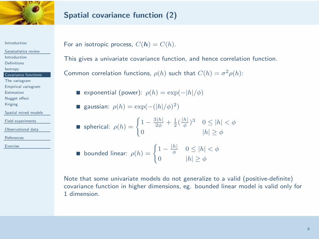
For an isotropic process, C(h) = C(h).

This gives a univariate covariance function, and hence correlation function.

Common correlation functions, ρ(h) such that C(h) = σ2ρ(h):

■ exponential (power): ρ(h) = exp(−|h|/φ)

■ gaussian: ρ(h) = exp(−(|h|/φ)2)

■ spherical: ρ(h) =

{

1 − 3|h|2φ

+ 12(|h|φ

)3 0 ≤ |h| < φ

0 |h| ≥ φ

■ bounded linear: ρ(h) =

{

1 − |h|φ

0 ≤ |h| < φ

0 |h| ≥ φ

Note that some univariate models do not generalize to a valid (positive-definite)covariance function in higher dimensions, eg. bounded linear model is valid only for1 dimension.

Spatial covariance function (3)

Introduction


Introduction

Definitions

Isotropy


The variogram

Empirical variogram

Estimation

Nugget effect

Kriging


Field experiments

Observational data

References

Exercise

10

Note that:

■ the exponential model is a generalization of the auto-regressive (AR) processto non-integer (and multi-dimensional) lags, since ρ(h) = θ|h| whereθ = e−1/φ

■ the bounded linear and spherical correlation functions have a finite range andare zero for |h| > φ

■ the exponential and gaussian models are zero only in the limit as |h| → ∞,but are effectively zero (close to zero) at finite distances

We will also briefly consider the Matern correlation function, defined by

ρ(h; ζ, ν) =1

2ν−1Γ(ν)

(

h

ζ

)ν

Kν

(

h

ζ

)

where Γ() is the Gamma function and Kν() is the modified Bessel function of thethird order.

This Bessel function takes a simple form for ν = m + 12

with m ∈ Z+ (see Haskard,

2007, for details).

Matern correlation function

Introduction


Introduction

Definitions

Isotropy


The variogram

Empirical variogram

Estimation

Nugget effect

Kriging


Field experiments

Observational data

References

Exercise

11

Special cases of the Matern correlation function occur for

■ ν = 12: ρ(h; ζ, ν = 1

2) = e−h/ζ ie. exponential correlation function

■ ν = 32: ρ(h; ζ, ν = 3

2) = e−h/ζ

(

hζ

+ 1)

■ ν = 52: ρ(h; ζ, ν = 5

2) = e−h/ζ

{

13

(

hζ

)2+ h

ζ+ 1

}

■ if ν → ∞ with ζ → 0 such that β = 2ν1/2ζ remains constant, thenρ(h; β) = exp(−(h/β)2), ie. gaussian correlation function

The Matern correlation function is therefore a generalization of several commoncorrelation functions. Its parameters can be interpreted as

■ ν, the smoothness of the spatial process (smoothness increases with ν)

■ ζ, the range of the correlation function

Note that the physical distance at which correlation decays to a given valuedepends upon both ν and ζ.

Separability

Introduction


Introduction

Definitions

Isotropy


The variogram

Empirical variogram

Estimation

Nugget effect

Kriging


Field experiments

Observational data

References

Exercise

12

If we can write

h =

(

h1

h2

)

then the spatial correlation function is called separable if it can be written as

ρ(h) = ρ1(h1)ρ2(h2).

So the covariance function is a simple product of the composite correlationfunctions.

This corresponds to the case of two independent processes in different directions.

The variogram

Introduction


Introduction

Definitions

Isotropy


The variogram

Empirical variogram

Estimation

Nugget effect

Kriging


Field experiments

Observational data

References

Exercise

13

The variogram only exists for a spatial process with intrinsic stationarity, and isdefined as

γ(h) =1

2var (y(s + h) − y(s)) .

Because of the multiplier, this function was historically called the semi-variogram.

Note that this function γ() is not the variance ratios used elsewhere.

With intrinsic stationarity

γ(h) =1

2V (s + h) +

1

2V (s) − C(h)

where V (si) is the variance of the process at position si.

With (second-order) stationarity

γ(h) =1

2C(0) +

1

2C(0) − C(h)

= C(0) − C(h)

= C(0)

(

1 − C(h)

C(0)

)

= σ2(1 − ρ(h))

Features of variograms

Introduction


Introduction

Definitions

Isotropy


The variogram

Empirical variogram

Estimation

Nugget effect

Kriging


Field experiments

Observational data

References

Exercise

14

0

0

a. Spherical+nugget

Separation distance

Sem

ivar

iogr

am

range

sill

nugget variance

0

0

b. Exponential+nugget

Separation distance

Sem

ivar

iogr

am

effective

range

sill0.95*sill

nugget variance

0

0

c. Gaussian+nugget

Separation distance

Sem

ivar

iogr

am

effective

range

sill0.95*sill

nugget variance

Figure 1: Fig 2.2 from Haskard (2007)

■ sill = value at which variogram levels off

■ range = lag at which the variogram reaches the sill

■ effective range = 95% of the sill

■ nugget variance = value of variogram at distance 0

Features of variograms (2)

Introduction


Introduction

Definitions

Isotropy


The variogram

Empirical variogram

Estimation

Nugget effect

Kriging


Field experiments

Observational data

References

Exercise

15

Anisotropy:

■ implies different variograms in different directions

■ usually assume common variances (hence sill) in different directions

■ usually assume different ranges may apply in different directions

■ can look at variogram in two directions directly or calculate severalone-dimensional variograms in different directions

Nugget effect:

■ spatial separation ↓ 0 but variogram does not decrease to zero

■ but γ(0) = 0 by definition

■ we will return to this

Features of variograms (3)

Introduction


Introduction

Definitions

Isotropy


The variogram

Empirical variogram

Estimation

Nugget effect

Kriging


Field experiments

Observational data

References

Exercise

16

xsep

ysep

Variogram

a.

xsep

ysep

Variogram

b.

xsep

ysep

Variogram

c.

0

0

d.

Separation distance

Dire

ctio

nal v

ario

gram

s

Direction

0o

45o

60o

90o

135o

150o

commonsill

Figure 2: Fig 2.3 from Haskard (2007)

Empirical variogram

Introduction


Introduction

Definitions

Isotropy


The variogram

Empirical variogram

Estimation

Nugget effect

Kriging


Field experiments

Observational data

References

Exercise

17

The empirical semi-variance between two points is defined as

1

2{y(si) − y(sj)}2

The variogram at lag h can be defined as

E

[

1

2{y(si) − y(sj)}2

]

with the expectation taken across all possible pairs si, sj with h = si − sj .

The empirical variogram at lag h is estimated by the mean taken across all pointpairs at lag h, or within a given neighbourhood of h:

■ the amount of information (number of point pairs) in the variogram at anydistance depends on the structure of the sample

■ number of available point pairs decreases as lag distance increases in anydirection

■ by convention, curtail the use empirical variogram at distances greater thanhalf the range of the original sample area

Estimating the spatial correlation function

Introduction


Introduction

Definitions

Isotropy


The variogram

Empirical variogram

Estimation

Nugget effect

Kriging


Field experiments

Observational data

References

Exercise

18

In traditional geo-statistics, the form of the spatial correlation function is estimatedfrom the variogram

■ either by eye

■ or by weighted least squares

Fitting the variogram to a standard parametric model allows interpolation ofcorrelation to spatial lags not present in the sample.

Neither of these estimation methods accounts for the correlations inherent in theempirical variogram, as each observed sample contributes to many neighbouringpoints in the variogram (up to n − 1 points).

This correlation makes the empirical variogram much smoother than might beexpected.

This method does not take account of sampling uncertainty in the empiricalvariogram.

Examples of variograms

Introduction


Introduction

Definitions

Isotropy


The variogram

Empirical variogram

Estimation

Nugget effect

Kriging


Field experiments

Observational data

References

Exercise

19

Figure 3: Data and variograms for pure noise y ∼ N(0, I100). Top left: exampledata. Other panes: variograms for independent samples.

Examples of variograms (2)

Introduction


Introduction

Definitions

Isotropy


The variogram

Empirical variogram

Estimation

Nugget effect

Kriging


Field experiments

Observational data

References

Exercise

20

Figure 4: Data and variograms for trend plus noise y ∼ N(0.025x, I100) for x =(1 . . . 100)′. Top left: example data. Other panes: variograms for independentsamples.


Introduction


Introduction

Definitions

Isotropy


The variogram

Empirical variogram

Estimation

Nugget effect

Kriging


Field experiments

Observational data

References

Exercise

21

Figure 5: Data and variograms for auto-regressive error with correlation 0.7 at lag 1,y ∼ N(0.025x, C). Top left: example data. Other panes: variograms for indepen-dent samples.


Introduction


Introduction

Definitions

Isotropy


The variogram

Empirical variogram

Estimation

Nugget effect

Kriging


Field experiments

Observational data

References

Exercise

22

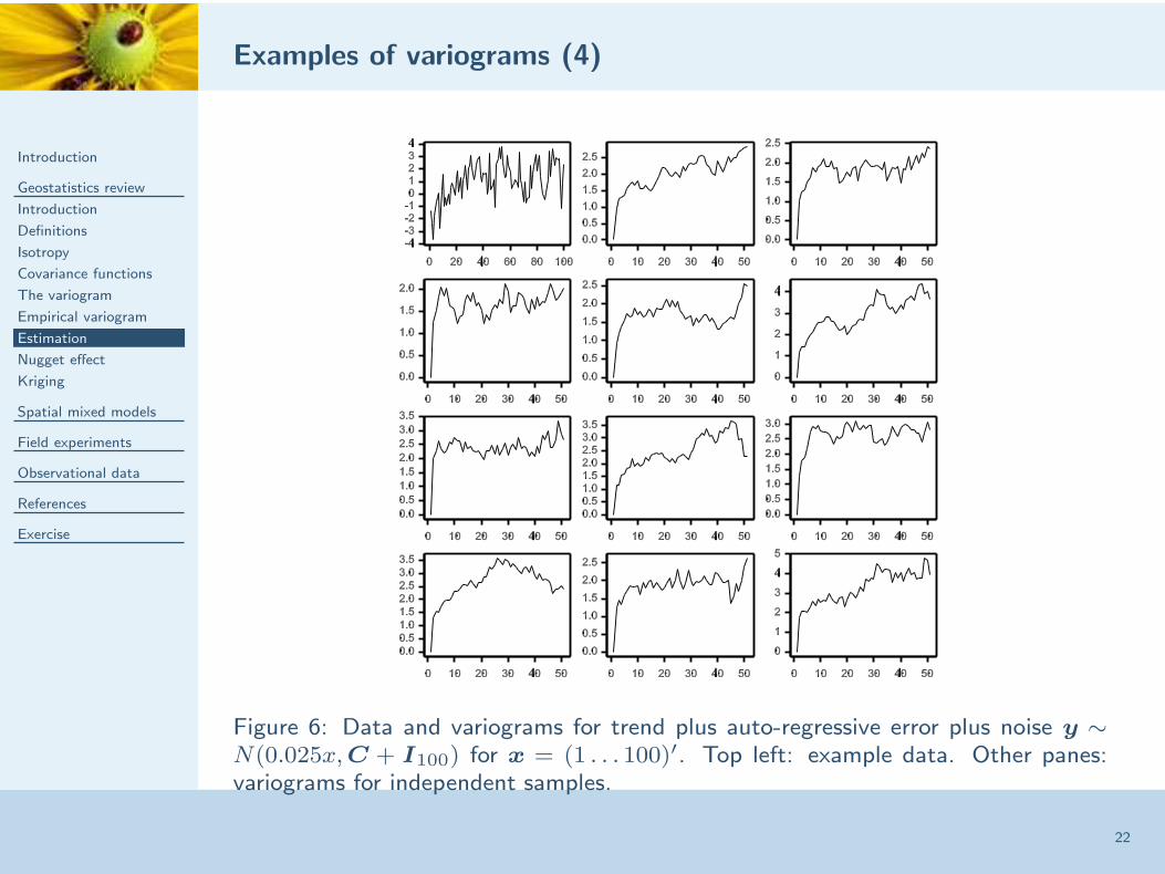
Figure 6: Data and variograms for trend plus auto-regressive error plus noise y ∼N(0.025x, C + I100) for x = (1 . . . 100)′. Top left: example data. Other panes:variograms for independent samples.

Nugget effect

Introduction


Introduction

Definitions

Isotropy


The variogram

Empirical variogram

Estimation

Nugget effect

Kriging


Field experiments

Observational data

References

Exercise

23

The nugget effect describes a non-zero value of the variogram at the origin (lag 0),contrary to the definition γ(0) = 0.

In general, the use of a nugget effect can be controversial, as it is estimated fromthe variogram and the smallest lag distance may be far from the origin.

The nugget variance is estimated by extrapolation of the variogram to the origin,which is done (in the absence of replication) without real information on the truevalue.

Causes of a nugget effect include

■ small range spatial process (range smaller than sampling distance)

■ measurement error

In general, we cannot distinguish the two sources of variation.

We can make some progress by taking replicate measurements

■ separate samples within a single location - gives information on small rangevariation

■ repeated measurement of a single sample (technical replication) givesinformation on measurement error

Kriging

Introduction


Introduction

Definitions

Isotropy


The variogram

Empirical variogram

Estimation

Nugget effect

Kriging


Field experiments

Observational data

References

Exercise

24

Kriging is the term used for prediction at locations unobserved in the sample,y(sp) = yp.

The principle of prediction used is BLUP = best (minimum MSE) linear unbiasedprediction.

A linear prediction must take the form

yp = λ0 +n∑

i=1

λiy(si)

hence, with second-order stationarity,

E

(

λ0 +n∑

i=1

λiy(si)

)

= λ0 +n∑

i=1

λiµ.

Unbiasedness requires E(yp) = µ ie.

µ = λ0 +n∑

i=1

λiµ ⇒ λ0 = (1 −n∑

i=1

λi)µ

which is solved by λ0 = 0 and∑n

i=1 λi = 1.

Kriging (2)

Introduction


Introduction

Definitions

Isotropy


The variogram

Empirical variogram

Estimation

Nugget effect

Kriging


Field experiments

Observational data

References

Exercise

25

Consider the square error on the predictor:

(yp − yp)2 = (yp − µ + µ − yp)2

= (n∑

i=1

λiyi − µ + µ − yp)2

= (n∑

i=1

λi(yi − µ))2 + 2(µ − yp)n∑

i=1

(λi(yi − µ)) + (µ − yp)2

=n∑

i,j=1

λiλj(yi − µ)(yj − µ)) + 2n∑

i=1

λi(yi − µ)(µ − yp) + (µ − yp)2

using∑n

i=1 λi = 1, hence

E(yp − yp)2 =n∑

i,j=1

λiλjcov (yi, yj) − 2n∑

i=1

λicov (yi, yp) + var (yp)

= var (yp) − 2λc + λ′V λ

where c = (cov (y1, yp) . . . cov (yn, yp))′ and V is the sample variance-covariancematrix.

Kriging (3)

Introduction


Introduction

Definitions

Isotropy


The variogram

Empirical variogram

Estimation

Nugget effect

Kriging


Field experiments

Observational data

References

Exercise

26

We need to maximise the mean squared error subject to the constraint λ′1 = 1,

which we do using Lagrange multipliers, hence we minimize

var (yp) − 2λc + λ′V λ− 2φ(λ′1 − 1)

Differentiate with respect to parameters λ and φ and set equal to zero:

−2c + 2V λ− 2φ1 = 0

⇒ V λ− φ1 = 0

andλ′

1 = 0

or, in matrix form,[

V 1

1′ 0

] (

λ

φ

) (

c

1

)

and by inverting the partitioned matrix:

λ = V −1

(

I − 11′V −1

1′V 1

)

c +V −1

1

1′V 1

Kriging (4)

Introduction


Introduction

Definitions

Isotropy


The variogram

Empirical variogram

Estimation

Nugget effect

Kriging


Field experiments

Observational data

References

Exercise

27

The kriging variance is defined as

var (yp − yp) = var(

λ′y − yp)

= var(λ′y) − 2cov(

λ′y, yp)

+ var (yp)

= λ′V λ− 2λ′c + var (yp)

which is exactly the mean squared error that has been minimized across all possibleestimators. Using

λ′V λ = c′V −1c− c′V −111

′V −1c

1′V −1

1+

1

1′V −1

1

2λ′c = 2c′V −1c− 2c′V −1

11′V −1c

1′V −1

1+ 2

1′V −1c

1′V −1

1

the kriging variance can be written as

var (yp − yp) = var (yp) − 2λ′c + λ′V λ

= var (yp) − c′V −1c +c′V −1

11′V −1c

1′V −11

− 21′V −1c

1′V −11

+1

1′V −11

= var (yp) − c′V −1c +(1 − 1

′V −1c)2

1′V −1

1

Spatial linear mixed model

Introduction



Kriging variance

Field experiments

Observational data

References

Exercise

28

Consider a linear mixed model for the spatial sample y of the form

y = µ1 + Zu + e

where var (u) = σ2G and var (e) = σ2R, and

V = var (y) = σ2(ZGZ′ + R)

is a stationary variance structure.

Consider a BLUP for a location not observed within the original sample:

yp = µ + zpup + ep

We know that, when using REML, u = E(u|L′2y) = GZ′Py and

e = E(e|L′2y) = RPy where L′

2X = 0.

So consider E(yp|L′2y):

E(yp|L′2y) = E[yp] + cov

(

yp, L′2y)

[var(

L′2y)

]−1L′2y

and usecov

(

yp, L′2y)

= σ2(zpGpoZ′ + Rpo)L2

where σ2Gpo = cov (up, u) and σ2Rpo = cov (ep, e).

Spatial linear mixed model (2)

Introduction



Kriging variance

Field experiments

Observational data

References

Exercise

29

Hence

E(yp|L′2y) = µ + (zpGpoZ′ + Rpo)L2(L

′2HL2)

−1L′2y

= µ + (zpGpoZ′ + Rpo)Py

= µ + zpGpoG−1u + RpoR−1e

but µ is unknown and is replaced by its BLUE µ = 1′V −1y

1′V −11to get prediction

E(yp|L′2y) = µ + zpGpoG−1u + RpoR−1e

We want to compare this with the kriging estimate written in terms of c, so notethat

E(yp|L′2y) = µ + c′Py/σ2

where here P = σ2(

V −1 − V −111

′V −1

1′V −11

)

, so

E(yp|L′2y) =

1′V −1y

1′V −11

+ c′Py/σ2

=

(

1′V −1

1′V −1

1+ c′

[

I − V −111

′

1′V −1

1

]

V −1

)

y = λ′y


Introduction



Kriging variance

Field experiments

Observational data

References

Exercise

30

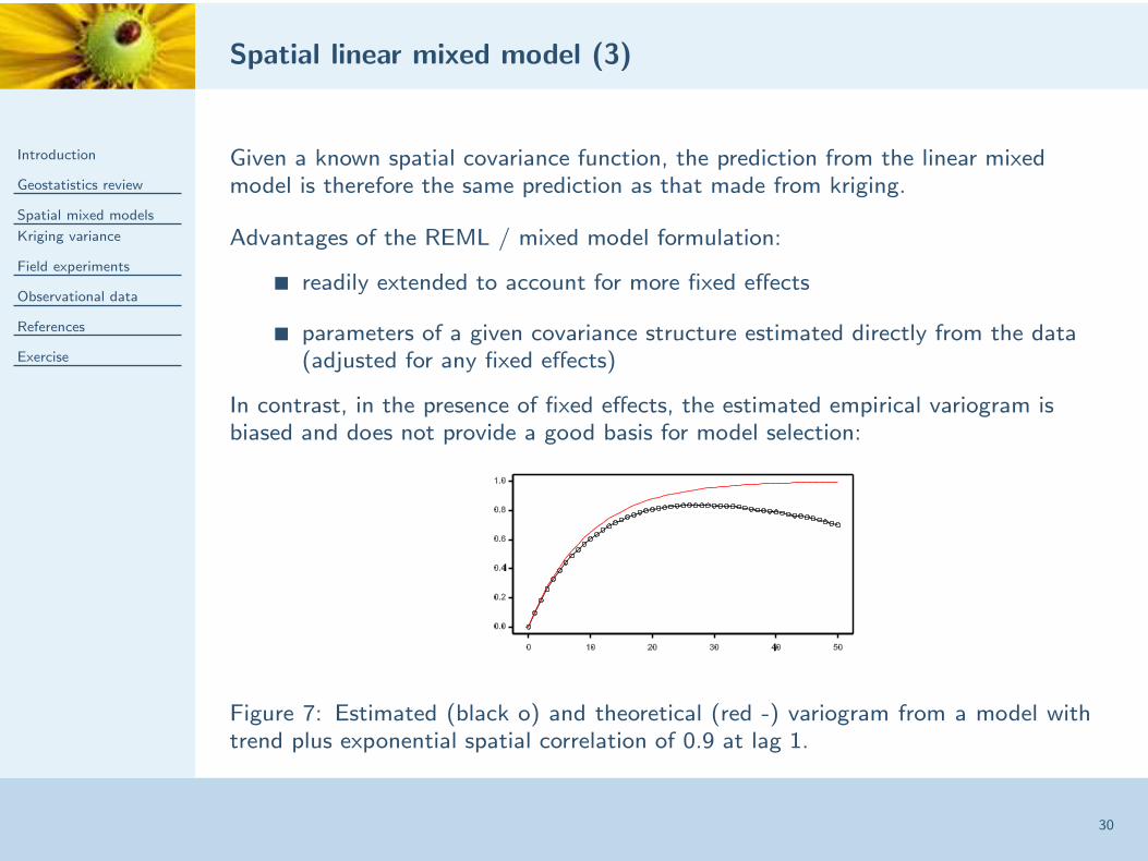
Given a known spatial covariance function, the prediction from the linear mixedmodel is therefore the same prediction as that made from kriging.

Advantages of the REML / mixed model formulation:

■ readily extended to account for more fixed effects

■ parameters of a given covariance structure estimated directly from the data(adjusted for any fixed effects)

In contrast, in the presence of fixed effects, the estimated empirical variogram isbiased and does not provide a good basis for model selection:

Figure 7: Estimated (black o) and theoretical (red -) variogram from a model withtrend plus exponential spatial correlation of 0.9 at lag 1.


Introduction



Kriging variance

Field experiments

Observational data

References

Exercise

31

The role of the variogram in the linear mixed model differs from geo-statistics:

■ in geo-statistics, the correlation function is often estimated from thevariogram

■ in the linear mixed model, parameters of a correlation function are estimateddirectly from the data

Given the bias of the empirical variogram in the presence of fixed effects, it arguablyhas no useful role in estimation.

Several authors find it useful to use the variogram as a diagnostic tool, either tosuggest a suitable correlation function or to find lack of fit.


Introduction



Kriging variance

Field experiments

Observational data

References

Exercise

32

Within the mixed model, there is a partition of random effects between u and e

(the residual term, which must be present).

For random terms with Z 6= I, there is only one allocation.

If there is only one random term with Z = I, then this must be the residual term.

If there are several terms with Z = I, then in theory they may be combined as acomposite residual term.

In practice, most software requires the residual to consist of a single term.

Special cases:

■ spatial model with replicate measurements but no independent error

◆ then Z 6= In so the model has no residual

■ spatial model plus independent error with no replication - either term couldbe used as the residual

Kriging variance

Introduction



Kriging variance

Field experiments

Observational data

References

Exercise

33

For a general modely = Xτ + Zu + e

and a predictionyp = xpτ + zpup + ep

it is helpful to consider the form of the kriging variance

var (yp − yp) = var (xp(τ − τ) + zp(up − up) + ep − ep)

= var(

xp(τ − τ) + zpGpoG−1(u− u) + RpoR−1(e− e)

+zpGpoG−1(u− up) + RpoR−1e− ep)

=

xp

zpGpoG−1

RpoR−1

var

τ − τ

u− u

e− e

xp

zpGpoG−1

RpoR−1

′

+σ2zp(Gpp − GpoG−1Gop)z′p + σ2(Rpp − RpoR−1Rop)

This variance can be interpreted as the sum of uncertainty in the estimates plusuncertainty due to spatial interpolation (prediction).

Kriging variance (2)

Introduction



Kriging variance

Field experiments

Observational data

References

Exercise

34

Special cases:

■ if prediction is at a point within the data set, cov (up, u) = 1 andcov (ep, e) = 1, then the fit is exact with no uncertainty in the prediction

■ if cov (up, u) = 0 and cov (ep, e) = 0, ie. independent random effects, thenGpo = 0 and Rpo = 0 hence

yp = xpτ

var (yp − yp) = xpvar (τ) x′p + σ2zpGppz′

p + σ2Rpp

ie. uncertainty due to fixed effects plus uncertainty due to unobservedrandom effects.

This use of prediction can be used to take into account uncertainty in futurerandom effects when making predictions.

Spatial analysis of field experiments

Introduction



Field experiments

Field experiments

Separability

2D variogram

Example

FE summary

Observational data

References

Exercise

35

■ Aim is to model spatial variation to get improved SEDs

■ Spatial models may be in conflict with randomization-based mixed model

■ e.g. small blocks can be effective approximation to smooth spatial trend

■ Danger of over-modelling variance pattern

Procedure suggested here based on Gilmour et al. (1997).

Modelling variation in field experiments as a sum of:

■ design-based blocking factors (to be retained as far as possible)

■ local natural trend (local spatial trend)

■ global natural trend (smooth trend across trial)

■ extraneous variation

Extraneous variation often associated with harvesting or sowing patterns, plottrimming, etc

Use of diagnostics (inc variogram) to detect different sources of error

Spatial analysis of field experiments

Introduction



Field experiments

Field experiments

Separability

2D variogram

Example

FE summary

Observational data

References

Exercise

36

■ Field experiments often laid out as a grid (rows × columns)

■ Field operations usually carried out in either row or column directions(sometimes alternating directions, i.e. up/down)

■ Shape of field has sometimes determined directions of operations onlong-term basis

■ So: many factors that may affect variation are closely associated with eitherrows or columns

We therefore often assume that the spatial process is separable between rows andcolumns, i.e. row processes act independently of column processes.

■ this seems realistic if we expect management practices to be the dominantform of spatial variation

■ but unrealistic if spatial variation is due to underlying environmentalconditions

Separability

Introduction



Field experiments

Field experiments

Separability

2D variogram

Example

FE summary

Observational data

References

Exercise

37

■ For data yij from row i and column j of the grid:

■ let y = (y11 y12 y13 . . . yrc)′ be the vector of data ordered as columnswithin rows

■ let Cr(φr) be the covariance structure across rows within any column

■ let Cc(φc) be the covariance structure across columns within any row

Separability implies that

var (y) = σ2Cr(φr) ⊗ Cc(φc)

■ simple model: two one-dimensional processes to consider

■ separability usually assumed rather than tested

■ departures from separability may be detected by variogram

■ two dimensional variogram required to account for separate row & columnprocesses

Two-dimensional variogram

Introduction



Field experiments

Field experiments

Separability

2D variogram

Example

FE summary

Observational data

References

Exercise

38

For a regular r × c grid, a two dimensional variogram can be defined.

Let eij be the residual from row i and column j.

Then vertices of the two-dimensional variogram are calculated as

V (s, t) =1

2(r − s)(c − t)

r−s∑

i=1

c−t∑

j=1

[ eij − ei+s,j+t ]2

■ should be able to see row/column variance pattern in edges of variogram(s = 0 or t = 0)

■ variogram should show no trend or systematic pattern

■ variogram should show regular behaviour consistent with separability

■ GenStat command f2dres [row=; column=] data= (also easy way of getting1D variograms for regular spacing)

Example: analysis of uniformity data

Introduction



Field experiments

Field experiments

Separability

2D variogram

Example

FE summary

Observational data

References

Exercise

39

■ Uniformity trial to investigate impact of field operations

■ Trial laid out as regular array 25 rows x 6 columns

■ Management practices aligned with rows and columns:

◆ trials sown by traversing columns in alternate directions

◆ using cone seeder which sows two plots at once with left or right side

◆ harvesting done in similar (but different) pattern to sowing

■ Gilmour et al. suggest starting with AR1 ⊗ AR1 model then usingdiagnostic plots to identify lack of fit

◆ plot of residuals against rows/columns for individual rows/columns ortogether

◆ two-dimensional variogram

■ procedure seems to work well in practice

GenStat specification

Introduction



Field experiments

Field experiments

Separability

2D variogram

Example

FE summary

Observational data

References

Exercise

40

"

Model 1: initial investigation of spatial pattern

=================================================

"

vcomp row.column

vstructure [row.column] factor=row,column; model=ar,ar

reml [prin=model,comp,dev] yield

vdis [prin=moni]

" Save residuals and look at patterns against rows/columns "

vkeep [residuals=res]

trellis [group=column; nrow=3; ncol=2] res; row; method=line

trellis res,res; row; method=point,mean

trellis [group=row] res; column; method=line

trellis res,res; column; method=point,mean

f2dres [row=row; col=column; title=’Variogram for AR1 x AR1’] res; variogram=var1

■ need to specify row.column residual term to apply variance model

■ for separable model, use direct product structure

Uniformity data

Introduction



Field experiments

Field experiments

Separability

2D variogram

Example

FE summary

Observational data

References

Exercise

41

Initial fit gives: σ2 = 0.06, φr = 0.25, φc = 0.44

Plot of residuals against row number within each column:

Uniformity data

Introduction



Field experiments

Field experiments

Separability

2D variogram

Example

FE summary

Observational data

References

Exercise

42

Plot of residuals against row number with mean:

Strong alternating pattern due to field operations.

Uniformity data

Introduction



Field experiments

Field experiments

Separability

2D variogram

Example

FE summary

Observational data

References

Exercise

43

Two-dimensional variogram from initial model

Alternating pattern dominates row direction.

Uniformity data

Introduction



Field experiments

Field experiments

Separability

2D variogram

Example

FE summary

Observational data

References

Exercise

44

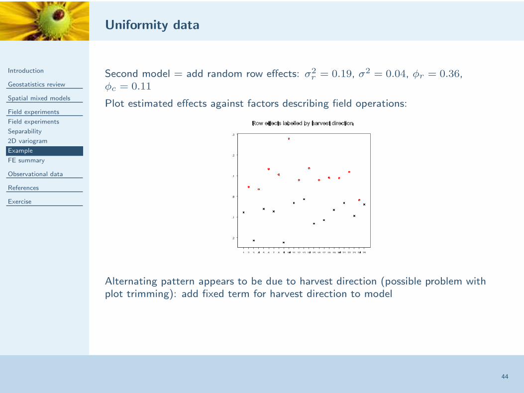
Second model = add random row effects: σ2r = 0.19, σ2 = 0.04, φr = 0.36,

φc = 0.11

Plot estimated effects against factors describing field operations:

Alternating pattern appears to be due to harvest direction (possible problem withplot trimming): add fixed term for harvest direction to model

Uniformity data

Introduction



Field experiments

Field experiments

Separability

2D variogram

Example

FE summary

Observational data

References

Exercise

45

Variogram now much improved:

Might try adding row and column random effects to take account of remainingsystematic pattern in variogram (and residual plots)

Use comparison of AIC or BIC to formally select model.

Uniformity data

Introduction



Field experiments

Field experiments

Separability

2D variogram

Example

FE summary

Observational data

References

Exercise

46

Use AIC/BIC to refine model: all models include harvest direction as fixed effects

Variance component Residual AR correlation −2RL Nv AIC BICRow Column Variance Row Column0 0 0.042 0 0 -313.83 1 -311.83 -308.83

0.005 0.012 0.027 0 0 -350.21 3 -344.21 -335.210 0 0.043 0.35 0.17 -331.42 3 -325.42 -316.42

0.003 0 0.040 0.36 0.10 -332.55 4 -324.55 -312.550 0.012 0.032 0.10 0.19 -348.64 4 -340.64 -328.64

0.004 0.012 0.027 0.07 0.06 -350.76 5 -340.76 -325.76

Note duality between main effects and correlations

■ including row main effect decreases column AR parameter

■ including column main effect decreases row AR parameter

■ exactly the same phenomena as noted for longitudinal data: random maineffects induce correlation within same level of factor

Field experiments: summary

Introduction



Field experiments

Field experiments

Separability

2D variogram

Example

FE summary

Observational data

References

Exercise

47

Suggested procedure is iterative:

■ try model → check residuals → try new model

■ then formalize choice using AIC/BIC

■ difficult to justify formally, seems to work in practice

In this example, there was no evidence of global trend

■ can take out trend using polynomials or smoothing splines

Real danger of over-modelling:

■ be wary of uncertainty in variograms / residual plots

■ use of BIC gives some protection

■ be aware of role of design-based factors in model (pragmatism)

Linear mixed models for observational data

Introduction



Field experiments

Observational data

Example

References

Exercise

48

Aim: to quantify influence of environmental factors on aphid occurrence in traps.

Scope of project:

■ environmental factors: climate, land use and pollution

■ trap positions across Western Europe

■ data for 35 years (mainly UK in first 10 years)

■ here: pilot study using a subset of trap data from the UK from 1965-1998,climate and land use data only

Spatial analysis

Introduction



Field experiments

Observational data

Example

References

Exercise

49

Aims of analysis:

■ use (linear) regression to model relationship between aphid variables andenvironment

■ investigate spatial trend in aphid variables not accounted for byenvironmental variables

Note: geo-statistics usually works on a single (large) spatial sample: we have smallsamples within each year.

Features of analysis:

■ mixed models allow joint estimation of regression coefficients and spatialcorrelation

■ assuming spatial correlation is the same, can accumulate information acrossyears

■ can allow additional variation due to sites and/or years

■ can allow correlation across years (independent of spatial correlation)

■ REML estimation of variance parameters

Model

Introduction



Field experiments

Observational data

Example

References

Exercise

50

The proposed model uses

■ fixed terms for regression on environmental variables

■ variance components for site and year

■ direct product correlation structure with independence across years, spatialcorrelation (C) across sites within years

Model is written:yij = Xτ + ti + sj + vij + ηij

where

■ yij is the data in year i (i=1 . . . m) at trap j (j=1 . . . n), ordered as siteswithin years

■ Xτ represents regression terms (fixed)

■ ti is the effect for year i, with var (t) = σ2Y Im

■ sj is the effect for trap j, var (s) = σ2SIn

■ vij is spatially correlated variation, var (v) = σ2vIm ⊗ C

■ ηij is additional independent sampling error, var (η) = σ2Imn

Random model

Introduction



Field experiments

Observational data

Example

References

Exercise

51

yij = Xτ + ti + sj + vij + ηij

Independent year effects (t) allow for effect of season that applies across all sites

■ does not help prediction in new years, might be explained by year-levelvariables

Independent site effects (s) allow for consistent effect at each site across years

■ does not help prediction at new sites, might be explained by site-levelvariables

Spatial correlation (v) allows for smooth spatial trend within each year

■ can predict at new sites within years where data available, explained bysite.year variables

Random error (η) - sampling variation.

Models for spatial correlation

Introduction



Field experiments

Observational data

Example

References

Exercise

52

Correlation across sites is based on distance between sites (exponential model).

For data at sites A (at location (xa, ya)′) and B (at location (xb, yb)′) the

correlation within year is modelled either as

■ C(A, B) = φ|xa−xb|x φ

|ya−yb|y (anisotropic model)

■ C(A, B) = φ(|xa−xb|+|ya−yb|) (isotropic model, city-block distances)

■ C(A, B) = φ√

(|xa−xb|2+|ya−yb|

2) (isotropic model, Euclidean distances)

where in all cases 0 ≤ φ, φx, φy ≤ 1.

For these models, the correlation decreases smoothly with distance, the parameterφ is the correlation at a distance of 1 unit in given direction (1 unit = 160km).

First model: look at variation without taking account of environmental variables

■ leaving out fixed effects changes values of variance parameters

■ not generally advisable - here, may give insight into baseline size and sourcesof variation due to environmental and site/year factors

■ can assess proportion of natural variation accounted for by environmentalvariables

Modelling strategy

Introduction



Field experiments

Observational data

Example

References

Exercise

53

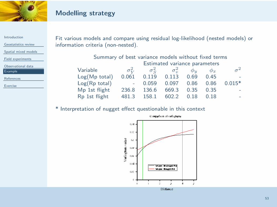
Fit various models and compare using residual log-likelihood (nested models) orinformation criteria (non-nested).

Summary of best variance models without fixed termsEstimated variance parameters

Variable σ2Y σ2

S σ2v φy φx σ2

Log(Mp total) 0.061 0.119 0.113 0.69 0.45 -Log(Rp total) - 0.059 0.097 0.86 0.86 0.015*Mp 1st flight 236.8 136.6 669.3 0.35 0.35 -Rp 1st flight 481.3 158.1 602.2 0.18 0.18 -

* Interpretation of nugget effect questionable in this context

Modelling strategy

Introduction



Field experiments

Observational data

Example

References

Exercise

54

Empirical variogram is probably consistent with either model - experience of thedata supports presence of large sampling variation.

Introduction



Field experiments

Observational data

Example

References

Exercise

55

Examination of the trap effects suggests that there is some dependence onenvironmental effects, here altitude.

Mixed model with environmental covariates

Introduction



Field experiments

Observational data

Example

References

Exercise

56

Limited set of covariates:

■ site position: longitude (X), latitude (Y), altitude (Z)

■ climate: Jan/Feb temperature, Jan/Feb rainfall

■ landscape: area of potatoes, oilseed rape or sugar beet in 50 km2

Modelling strategy

■ fit all covariates, reselect random model

■ drop unimportant fixed variables (Wald tests)

■ not robust procedure with respect to variable selection, return to this later

■ chosen variables: X, Y, Y2, Z, osr

Model summary

Introduction



Field experiments

Observational data

Example

References

Exercise

57

Comparison of variance models excluding and including environmental variables:

-/+ Estimated variance parameterscovariates Variable σ2

Y σ2S σ2

v φy φx σ2

- Log(Mp total) 0.061 0.119 0.113 0.69 0.45 -+ Log(Mp total) 0.053 0.003 0.113 0.70 0.46 -- Log(Rp total) - 0.059 0.097 0.86 0.86 0.015+ Log(Rp total) - 0.010 0.087 0.83 0.83 0.014- Mp 1st flight 236.8 136.6 669.3 0.35 0.35 -+ Mp 1st flight - - 639.0 0.32 0.32 -- Rp 1st flight 481.3 158.1 602.2 0.18 0.18 -+ Rp 1st flight 102.4 - 649.1 0.19 0.19 -

■ independent site and year variation greatly reduced

■ site.year spatial variation not reduced by addition of covariates

■ site.year level covariates (climate and landuse) turn out to have year+siteadditive structure

Prediction/kriging

Introduction



Field experiments

Observational data

Example

References

Exercise

58

Predictions at unobserved locations (kriging) are made using all terms:

This surface is more complex than could be predicted using the fixed terms only.

References / Further reading

Introduction



Field experiments

Observational data

References

References

Exercise

59

Cressie, N. A. C. (1993) Analysis of spatial data John Wiley & Sons, New York.

Gilmour, A. R. and Cullis, B. R. and Verbyla, A. P. (1997) Accounting for naturaland extraneous variation in the analysis of field experiments. Journal of Agricultural,Biological, and Environmental Statistics, 2, 269–273.

Haskard, K.A. (2007) An isotropic Matern spatial covariance model: REML estimation andproperties. PhD thesis, University of Adelaide.

Lark, R.M., Cullis, B.R, & Welham, S.J. (2006) On spatial prediction of soil propertiesin the presence of a spatial trend: the empirical best linear unbiased predictor(E-BLUP) with REML. European Journal of Soil Science, 57, 787-799.

Exercise

Introduction



Field experiments

Observational data

References

Exercise

Exercise

60

Field experiment with spatial trend:

■ Laid out as grid of 16 rows × 6 columns

■ Tests 8 varieties at 6 seedrates with 2 reps

■ Rep 1 = columns 1-3, rep 2 = columns 4-6

■ data held in spreadsheet yield.xls

Try to find a sensible model for this data.

reml estimation and linear mixed models 4. geostatistics ... · geostatistics is concerned with the...

Documents