reliable estimation of membrane curvature for cryo

RESEARCH ARTICLE

Reliable estimation of membrane curvature

for cryo-electron tomography

Maria SalferID1,2, Javier F. ColladoID

1,2,3, Wolfgang Baumeister1, Ruben Fernandez-

BusnadiegoID1,3,4, Antonio Martınez-SanchezID

1,3,4*

1 Department of Molecular Structural Biology, Max Planck Institute of Biochemistry, Martinsried, Germany,

2 Graduate School of Quantitative Biosciences Munich, Munich, Germany, 3 Institute of Neuropathology,

University Medical Center Gottingen, Gottingen, Germany, 4 Cluster of Excellence “Multiscale Bioimaging:

from Molecular Machines to Networks of Excitable Cells” (MBExC), University of Gottingen, Germany

* [email protected], [email protected]

Abstract

Curvature is a fundamental morphological descriptor of cellular membranes. Cryo-electron

tomography (cryo-ET) is particularly well-suited to visualize and analyze membrane mor-

phology in a close-to-native state and molecular resolution. However, current curvature esti-

mation methods cannot be applied directly to membrane segmentations in cryo-ET, as

these methods cannot cope with some of the artifacts introduced during image acquisition

and membrane segmentation, such as quantization noise and open borders. Here, we

developed and implemented a Python package for membrane curvature estimation from

tomogram segmentations, which we named PyCurv. From a membrane segmentation, a

signed surface (triangle mesh) is first extracted. The triangle mesh is then represented by a

graph, which facilitates finding neighboring triangles and the calculation of geodesic dis-

tances necessary for local curvature estimation. PyCurv estimates curvature based on ten-

sor voting. Beside curvatures, this algorithm also provides robust estimations of surface

normals and principal directions. We tested PyCurv and three well-established methods on

benchmark surfaces and biological data. This revealed the superior performance of PyCurv

not only for cryo-ET, but also for data generated by other techniques such as light micros-

copy and magnetic resonance imaging. Altogether, PyCurv is a versatile open-source soft-

ware to reliably estimate curvature of membranes and other surfaces in a wide variety of

applications.

Author summary

Membrane curvature plays a central role in many cellular processes like cell division,

organelle shaping and membrane contact sites. While cryo-electron tomography (cryo-

ET) allows the visualization of cellular membranes in 3D at molecular resolution and

close-to-native conditions, there is a lack of computational methods to quantify mem-

brane curvature from cryo-ET data. Therefore, we developed a computational procedure

for membrane curvature estimation from tomogram segmentations and implemented it

in a software package called PyCurv. PyCurv converts a membrane segmentation, i.e. a set

PLOS COMPUTATIONAL BIOLOGY

PLOS Computational Biology | https://doi.org/10.1371/journal.pcbi.1007962 August 10, 2020 1 / 29

a1111111111

a1111111111

a1111111111

a1111111111

a1111111111

OPEN ACCESS

Citation: Salfer M, Collado JF, Baumeister W,

Fernandez-Busnadiego R, Martınez-Sanchez A

(2020) Reliable estimation of membrane curvature

for cryo-electron tomography. PLoS Comput Biol

16(8): e1007962. https://doi.org/10.1371/journal.

pcbi.1007962

Editor: Jeffrey J. Saucerman, University of Virginia,

UNITED STATES

Received: October 30, 2019

Accepted: May 18, 2020

Published: August 10, 2020

Copyright: © 2020 Salfer et al. This is an open

access article distributed under the terms of the

Creative Commons Attribution License, which

permits unrestricted use, distribution, and

reproduction in any medium, provided the original

author and source are credited.

Data Availability Statement: The algorithms and

experimental data are publicly available in a

software package called PyCurv at https://github.

com/kalemaria/pycurv. Tomograms and

segmentations in Figs 2, 11 and 12 have been

deposited EM Data Bank (EMD-10767, EMD-

10765, and EMD-10766).

Funding: MS and JC have been supported by the

Graduate School of Quantitative Biosciences

Munich GSC-1006 (http://qbm.genzentrum.lmu.

de). MS, JC, WB, RF-B, and AM-S have received

http://orcid.org/0000-0002-7604-6617

http://orcid.org/0000-0002-8707-6619

http://orcid.org/0000-0002-8366-7622

http://orcid.org/0000-0002-5865-2138

https://doi.org/10.1371/journal.pcbi.1007962

http://crossmark.crossref.org/dialog/?doi=10.1371/journal.pcbi.1007962&domain=pdf&date_stamp=2020-08-20








http://creativecommons.org/licenses/by/4.0/

https://github.com/kalemaria/pycurv


http://qbm.genzentrum.lmu.de

http://qbm.genzentrum.lmu.de

of voxels, into a surface, i.e. a mesh of triangles. PyCurv uses the local geometrical infor-

mation to reliably estimate the local surface orientation, the principal (maximum and

minimum) curvatures and their directions. PyCurv outperforms well-established curva-

ture estimation methods, and it can also be applied to data generated by other imaging

techniques.

This is a PLOS Computational Biology Methods paper.

Introduction

Membranes define the limits of the cells and encompass compartments within eukaryotic

cells, helping to maintain specific micro-environments with different shapes and functions.

Membrane curvature is important for many cellular processes, including organelle shaping,

vesicle formation, scission and fusion, protein sorting and enzyme activation [1, 2]. There is a

plethora of cellular mechanisms for generation, sensing and maintenance of local membrane

curvature, e.g. clustering of conical lipids or transmembrane proteins, insertion of specific pro-

tein domains as well as larger scale scaffolding by e.g. cytoskeletal filaments [1, 3].

Cryo-electron tomography (cryo-ET) enables an accurate three-dimensional (3D) visualiza-

tion and analysis of the subcellular architecture at molecular resolution [4–6] and is particu-

larly well-suited to study membrane morphology. While other transmission electron

microscopy (TEM) techniques may cause membrane deformations by chemical fixation and

dehydration, cryo-ET allows imaging of fully hydrated vitrified cells in a close-to-native state

with minimal structural perturbations [7]. The nominal resolution of tomograms can reach

�2-4 Å per voxel, but tomograms are usually binned for membrane segmentation to enhance

contrast, resulting in voxel sizes of�0.8-1.6 nm. Subtomogram averaging allows to routinely

obtain structures in the 10-20 Å resolution range, although higher resolutions are in principle

attainable [8]. Cryo-ET can be used to study membrane morphology and curvature in recon-

stituted preparations [9–13] and intact cells [14, 15]. We have recently employed cryo-ET to

visualize peaks of extreme curvature on the cortical endoplasmic reticulum (cER) membrane

facing the plasma membrane (PM). These high curvature structures are formed by Tcb pro-

teins and help to maintain PM integrity under heat stress [16]. We have also used cryo-ET to

show that polyQ-expanded huntingtin exon I fibrils induce high curvature in the endoplasmic

reticulum (ER) membrane, perhaps leading to ER membrane disruption [17]. Since we lacked

a method to reliably quantify membrane curvature in noisy cryo-ET data, we developed a new

method, which we formally describe in this paper.

In cryo-ET, the vitreous sample is tilted around an axis inside the electron microscope,

while 2D images of a cellular region of interest are acquired for each tilt. The tilt series are then

computationally aligned and reconstructed into a tomogram, which is a 3D gray-value image

of the cellular interior. Because in practice it is unfeasible to tilt the sample beyond� ±60˚, in

single-tilt tomography there is a wedge of missing information in the Fourier space. This arti-

fact, called missing wedge [4], causes the features to look smeared out along the electron beam

direction (Z-axis), while surfaces perpendicular to the tilt axis (Y-axis) are not visible. Thus,

missing membrane regions appear at the top and the bottom of both the Y- and Z-axes.

Nevertheless, the missing wedge does not affect the automatically segmented membrane, the

PLOS COMPUTATIONAL BIOLOGY Membrane curvature in cryo-electron tomography


funds from the European Research Council FP7 GA

ERC-2012- 387 SyG_318987-ToPAG (http://erc.

europa.eu). AM-S and RF-B were supported by the

Deutsche Forschungsgemeinschaft (DFG, German

Research Foundation) under Germany’s Excellence

Strategy - EXC 2067/1-390729940 and the Lower

Saxony Ministry of Science and Culture. The

funders had no role in study design, data collection

and analysis, decision to publish, or preparation of

the manuscript.

Competing interests: The authors have declared

that no competing interests exist.


http://erc.europa.eu

http://erc.europa.eu

elongated regions are just omitted [18, 19]. Moreover in cryo-ET, the cells are illuminated by

only a low dose of electrons, resulting in tomograms of low signal-to-noise ratio. Segmenta-

tion, i.e. voxel labeling of structural components present in tomograms, is necessary for tomo-

gram interpretation. Available software packages can assist membrane segmentation [18, 20–

22], but in most cases human supervision is still necessary due to the complexity of the cellular

context and the low signal-to-noise ratio.

Currently, the interpretation of membrane segmentations is limited by the lack of computa-

tional methods to measure quantitative descriptors. Here, we quantitatively determine local

curvature descriptors of cellular membranes from tomogram segmentations. A membrane can

be modeled as a surface [23], so that curvature descriptors characterize its local geometry. For

a surface embedded in a 3D space, principal curvatures measure the maximum and minimum

bending at each point, while the principal directions define the directions of the principal cur-

vatures as orthogonal vectors embedded on the tangent plane to the surface at each point [24].

From the principal curvatures, both extrinsic (mean) and intrinsic (Gaussian) surface curva-

tures can be computed for each point.

An oriented triangle mesh is the most common way to represent discrete surfaces [25]. How-ever, triangle mesh generation from a set of voxels [26] is not trivial because of the presence ofholes in membrane segmentations. Besides the errors generated during membranesegmentation, quantization noise [27] is the limiting factor for describing local membrane geo-metry. The term quantization noise includes here all accuracy limiting factors induced by thediscretization of segmented data using binary voxels (1 membrane and 0 background). This bin-ary discretization leads to step-wise surfaces, since surface extraction algorithms would needgray levels to achieve subvoxel precision.

Curvature estimation algorithms can be divided into three main categories: discrete, analyt-

ical and based on tensor voting. Discrete algorithms use discretized formulae of differential

geometry, approximating a surface from a mesh [25, 28–31]. However, the majority of those

algorithms use only a 1-ring neighborhood, i.e. triangle vertices sharing an edge with the cen-

tral vertex, and therefore are not robust for coarsely triangulated, noisy surfaces [32]. An

exception is [31], which uses a geodesic neighborhood of a certain size. Moreover, discrete

algorithms do not directly estimate the principal directions or principal curvatures [33]. Ana-

lytical algorithms fit surfaces [32, 34] or curvature tensors [35–37] to local patches of the mesh,

defined by a central vertex and a small neighborhood around it, and derive principal curva-

tures and directions from their model. The surface fitting algorithms are more robust to noise

but more susceptible to surface discontinuities [33]. The last category of algorithms applies

Medioni’s tensor voting theory [38] on a neighborhood of an arbitrary size to fit curvature ten-

sors, increasing the robustness of principal directions and curvatures estimation for noisy sur-

faces with discontinuities [33, 39, 40]. However, [33] leads to wrong curvature sign estimation

for non-convex surfaces, while [39, 40] were designed for point clouds instead of triangle

meshes. While most of the algorithms operate on triangle vertices because the computation of

distances on surfaces is straightforward, some operate on triangle faces [31, 36, 37], exhibiting

a more robust behavior on irregularly tessellated and moderately noisy meshes.

Discrete curvature estimation algorithms are included in two software packages for analysis

of magnetic resonance imaging (MRI) data of the human brain: the widely used FreeSurfer

[41] and the newer Mindboggle [42]. Curvature of the interventricular septum in the heart

from MRI was estimated in 3D using smoothing 2D spline surfaces and differential geometry

operators [43]. However, those algorithms require strong smoothing of surfaces to achieve

robust results, which would lead to a loss of high resolution details present in cryo-ET data.

For microscopy data, there is software to study curvature of linear cellular structures like

microtubules [44], which is not applicable to surfaces. For fluorescence microscopy data,




smooth point cloud surfaces of cellular membranes were reconstructed and their curvatures

estimated based on local surface fitting [45]. Hoffman et al. [46] also used a local surface fitting

method to estimate membrane curvature from block-face electron microscopy data. However,

also these methods employ strong smoothing of surfaces, eliminating small structural details.

In cryo-ET, some membrane curvature approximation methods have been already proposed

[9, 14], but they only work on 2D slices and are not capable of measuring curvature on arbi-

trary membranes in 3D.

Here, we developed and implemented a method for robust membrane curvature estimation

from tomogram segmentations. In brief, the workflow has the following steps. (1) From a seg-

mentation, a single-layered, signed triangle mesh surface is extracted. (2) To extract the surface

topology, we generate a spatially embedded graph. Graph vertices depict triangle centers and

graph edges connect the centers of triangle pairs sharing an edge or a vertex. (3) Local curva-

ture descriptors are computed for every triangle center. We propose different procedures that

combine two established tensor voting-based algorithms [33, 40] but operate on triangle faces,

aiming to increase the robustness to membrane geometries present in cryo-ET and to mini-

mize the impact of quantization noise. Extensive evaluation of our algorithms and comparison

with three well-established ones [30, 41, 42] on synthetic and biological surfaces proved the

superiority of our approach in terms of accuracy and robustness to noise for cryo-ET and

other imaging techniques.

Materials and methods

Cryo-ET data collection and segmentation

As real-world test input files for PyCurv, in this study we used membrane segmentations from

in situ cryo-ET data collected from vitrified cells: a human HeLa cell [17], yeast Saccharomycescerevisiae (EMD-10767 and EMD-10765) and a primary mouse neuron (EMD-10766). The

cells were milled down to 150-250 nm thick lamellas using cryo-focused ion beam [16, 54] and

imaged using a Titan Krios cryo-electron microscope (FEI), equipped with a K2 Summit direct

electron detector (Gatan), operated in dose fractionation mode. Tilt series were recorded

using SerialEM software [55] at magnifications of 33,000 X (pixel size of 4.21 Å) for the HeLa

cell and the mouse neuron and 42,000 X (pixel size of 3.42 Å) for yeast, typically from -50˚ to

+60˚ with increments of 2˚. The K2 frames were aligned using K2Align software [56]. Tilt

series were aligned using patch-tracking and weighted back projection provided by the IMOD

software package [57]. The tomograms were binned 4 times to improve contrast prior to seg-

mentation, thus the voxel size of the final segmentations was 1.684 nm (HeLa cell and mouse

neuron) and 1.368 nm (yeast). The contrast of one tomogram of yeast (EMD-10767) was

enhanced prior to segmentation using an anisotropic filter [58], while the contrast of the other

tomogram of yeast (EMD-10765) and the one of the mouse neuron was enhanced using a

deconvolution filter executed in MATLAB (MathWorks) using the functionalities of the TOM

toolbox [59]. Membrane segmentations were generated automatically from tomograms using

TomoSegMemTV [18] using parameters s = 10 and t = 0.3 (HeLa cell), s = 12 and t = 4

(yeast) and s = 10 and t = 3 (mouse neuron) and further refined manually using Amira

Software (ThermoFisher Scientific). The lumen of membrane compartments was then filled

manually.

Data preprocessing algorithms

The first steps of the PyCurv workflow (Fig 1A) are the conversion of the input segmentation

into a surface and the extraction of its associated graph.



https://github.com/dtegunov/k2align

https://github.com/dtegunov/tom_deconv

https://github.com/dtegunov/tom_deconv

https://www.thermofisher.com/de/de/home/industrial/electron-microscopy/electron-microscopy-instruments-workflow-solutions/3d-visualization-analysis-software/amira-life-sciences-biomedical.html


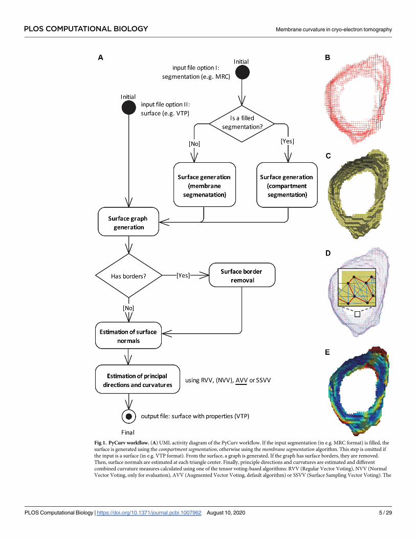
Fig 1. PyCurv workflow. (A) UML activity diagram of the PyCurv workflow. If the input segmentation (in e.g. MRC format) is filled, the

surface is generated using the compartment segmentation, otherwise using the membrane segmentation algorithm. This step is omitted if

the input is a surface (in e.g. VTP format). From the surface, a graph is generated. If the graph has surface borders, they are removed.

Then, surface normals are estimated at each triangle center. Finally, principle directions and curvatures are estimated and different

combined curvature measures calculated using one of the tensor voting-based algorithms: RVV (Regular Vector Voting), NVV (Normal

Vector Voting, only for evaluation), AVV (Augmented Vector Voting, default algorithm) or SSVV (Surface Sampling Vector Voting). The




Surface generation. A surface can be extracted using PyCurv from two types of input

segmentations, a membrane segmentation or a compartment segmentation. This step is not

required if the input is directly a surface (Fig 1A).

Using the membrane segmentation surface generation algorithm, the segmented membrane

of interest (Fig 2B) from the binned tomogram (Fig 2A) was used as the input for an algorithm

[26] that reconstructs signed, single-layered triangle-mesh surfaces from an unorganized set of

points, here the membrane voxels (Fig 1B). This algorithm was designed for closed surfaces

without boundaries. However, most segmented membranes in cryo-ET are open, e.g. due to

noise or missing wedge artifacts. Attempting to close the surface, the algorithm generated large

artefactual surface regions beyond the segmentation (Fig 2D, transparent white). These regions

were largely discarded by applying a mask with the membrane segmentation (Fig 2D, yellow).

Since the masking was done with a distance threshold of three voxels in order to bridge upon

small holes in the segmentation, additional three voxels-wide border remained. This additional

border was removed in the final cleaning step (see Surface graph generation). We use the con-

vention that normal vectors ("normals") point inwards in a convex surface. However, since

membrane segmentations have boundaries, the algorithm [26] sometimes mistakenly initiates

normals on both sides (Fig 2D, red arrows). As a result, ridge-like patches appear along the

surface (Fig 2E), leading to holes in the cleaned surface (Fig 2F). In some cases, the surface

reconstruction can be improved by closing small holes in the segmentation using morphologi-

cal operators.

The compartment segmentation surface generation algorithm requires additional segmenta-

tion of the inner volume of a compartment enclosed by a membrane (Fig 2C). This unequivo-

cally defines the orientation of the membrane by closing its holes. After joining the membrane

and its inner volume masks, we generate an isosurface around the resulting volume using the

Marching Cubes algorithm [47]. Finally, we apply a mask using the original membrane seg-

mentation to keep only the surface region going through the membrane (again, except for the

additional border that is cleaned in the end). The surface orientation is recovered perfectly in

our experiments (Fig 2G). In some cases, especially where the membrane segmentation was

manually refined, Marching Cubes produces triangles standing out perpendicularly to the sur-

face (Fig 2H), leading to holes in the cleaned surface (Fig 2I). To correct those artifacts and

exploit the subvoxel precision offered by Marching Cubes, the compartment segmentation

mask was slightly smoothed using a Gaussian kernel with σ = 1 voxel before extracting the sur-

face (Fig 2J–2L).

In summary, although compartment segmentations require more human intervention, they

ensure smoother and well oriented surfaces. Thus, we choose this algorithm as the default for

the subsequent data processing.

Surface graph generation. Curvature is a local property. Thus, for a triangle-mesh sur-

face, curvature has to be estimated using a local neighborhood of triangles. If the neighbor-

hood is too small, one would measure only noise created by the steps between voxels. If the

neighborhood is too large, one would underestimate the curvature.

To estimate geodesic distances within membrane surfaces, we use the graph-tool python

library [48] to map the triangle mesh (Fig 1A and 1C) into a spatially embedded graph, here

output is a surface with all the calculated values stored as triangle properties (VTP format). All the processing steps (rounded rectangles)

are implemented in PyCurv. (B) Voxels of a segmentation of a vesicle from a cryo-electron tomogram of a human HeLa cell [17]. (C) A

surface (triangle mesh) generated from the membrane segmentation shown in (A). (D) Surface graph generated from the surface shown in

(B); the inset shows a magnified region of the graph mapped on top of the triangle mesh (triangles: yellow, graph vertices: black dots,

strong edges: red lines, weak edges: light blue lines). (E) The output surface with estimated normals, principal directions and curvatures as

well as several combined curvature measures. Here, curvedness is shown. See also the video in S1 Video.

https://doi.org/10.1371/journal.pcbi.1007962.g001





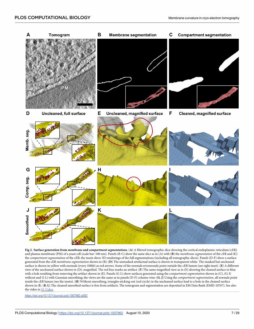
Fig 2. Surface generation from membrane and compartment segmentations. (A) A filtered tomographic slice showing the cortical endoplasmic reticulum (cER)

and plasma membrane (PM) of a yeast cell (scale bar: 100 nm). Panels (B-C) show the same slice as in (A) with (B) the membrane segmentation of the cER and (C)

the compartment segmentation of the cER; the insets show 3D renderings of the full segmentations (including all tomographic slices). Panels (D-F) show a surface

generated from the cER membrane segmentation shown in (B): (D) The unmasked artefactual surface is shown in transparent white. The masked but uncleaned

surface is shown in yellow with normals (every 100th) as red arrows. Some of the normals erroneously point outside the cER lumen (see right inset). (E) A different

view of the uncleaned surface shown in (D), magnified. The red line marks an artifact. (F) The same magnified view as in (E) showing the cleaned surface in blue

with a hole resulting from removing the artifact shown in (E). Panels (G-L) show surfaces generated using the compartment segmentation shown in (C), (G-I)

without and (J-L) with Gaussian smoothing; the views are the same as in panels (D-F) column-wise: (G, J) Using the compartment segmentation, all normals point

inside the cER lumen (see the insets). (H) Without smoothing, triangles sticking out (red circle) in the uncleaned surface lead to a hole in the cleaned surface

shown in (I). (K-L) The cleaned smoothed surface is free from artifacts. The tomogram and segmentation are deposited in EM Data Bank (EMD-10767). See also

the video in S1 Video.






referred as surface graph. First, graph vertices are associated to triangle centroid coordinates.

Second, pairs of triangles sharing two triangle vertices are connected by strong edges, while

those sharing only one triangle vertex are connected by weak edges (Fig 1D). To approximate

the shortest paths along the surface between the centers of a source triangle and a target trian-

gle, the graph is traversed starting from the source vertex along all its edges until the target ver-

tex is found, using the Dijkstra algorithm [49]. Using both strong and weak edges increases the

number of possible paths and thus improves the estimation of the shortest path. The geodesic

distance is computed by summing up the lengths of the edges comprising the shortest path.

Another application of the surface graph is to remove surface borders to avoid wrong cur-

vature estimations in these regions. Using the surface graph, we can detect triangles at borders

because they have less than three strong edges. Then, triangles up to a certain geodesic distance

from the border can be found and filtered out from the surface.

Curvature estimation algorithms

We estimate membrane curvature from surface graphs (Fig 1A). This algorithm combines two

previously published algorithms that are based on tensor voting and curvature tensor theory

[33, 40], to increase the precision of curvature estimation for noisy surfaces. To estimate prin-

cipal curvatures, principal directions have to be estimated. For the estimation of principal

directions, surface normals are required. Surface normals are robustly estimated by averaging

normals of triangles within a geodesic neighborhood.

Parameters defining the geodesic neighborhood. Similarly to [40], here we define a

radius_hit (rh) parameter to approximate the highest curvature value we can estimate

reliably, i.e. rh-1. For each surface triangle center, we define its local neighborhood as

gmax ¼p � rh

2; ð1Þ

where gmax defines the maximum geodesic distance. In Eq 1, gmax is approximated by one

quarter of a circle perimeter with radius equal to rh (Fig 3A).

Estimation of surface normals. Normals computed directly from the triangle mesh are

corrupted by quantization noise. To avoid this, we have adapted the first step of the algorithm

proposed in [33], but estimating the normals for each triangle center instead of defining new

normals at each triangle vertex.

For each triangle centroid (or graph vertex) v, the normal votes of all triangles within its

geodesic neighborhood are collected and the weighted covariance matrix sum Vv is calculated.

More precisely, a normal vote~ni of a neighboring triangle (whose center ci is lying within gmax

of vertex v) is calculated using the normal~nciassigned to this triangle:

~ni ¼ ~nciþ 2 cos yi

~vcik~vcik

; ð2Þ

where cos yi ¼ �~ntci ~vc ik~vc ik

,~ntci

is the transposed vector~nci, ~vc i ¼ ci � v and 0� θi� π. This for-

mula fits a smooth curve from ci to v, allowing the normal vote~ni to follow this curve, so that

the angle θi between~ni and ~vci is equal to the angle between~nciand -~vci. According to the per-

ceptual continuity constrain [38], the most appropriate curve is the shortest circular arc (Fig

3B). Then, each vote is represented by a covariance matrix Vi ¼ ~nti~ni, and votes from the geo-

desic neighborhood are collected as a weighted matrix sum Vv:

Vv ¼P

wiVi; ð3Þ




where wi is a weighting term calculated as follows:

wi ¼ai

amaxexp �

gis

� �: ð4Þ

The weight of the vote of a neighboring triangle increases linearly with its surface area ai, but

decreases exponentially with its geodesic distance gi to v. amax is the area of the largest triangle

in the whole surface and σ is an exponential decay parameter, which is set to fulfill 3σ = gmax,

so that votes beyond the geodesic neighborhood have almost no influence and can be ignored.

The votes collected into the matrix Vv are used for estimating the correct normal vector for

the triangle represented by vertex v. This is done by eigen-decomposition of Vv, which gener-

ates three real eigenvalues e1� e2� e3 with corresponding eigenvectors~e1,~e2 and~e3. The nor-

mal direction is equal in its absolute value to that of the first eigenvector. During construction

of Vv, the sign of normal votes is lost when Vi is computed. The correct orientation can be

recovered from the original normal~n, as the original surface was already oriented. Therefore,

Fig 3. Neighborhood parameters and voting geometry. (A) Schematic illustrating the rh and gmax parameters. gmaxis one quarter of the circle perimeter with radius equal to rh. gmax defines the maximum geodesic distance from a

surface triangle center to the centers of its neighboring triangles, approximated by the shortest path along the edges of

the surface graph. (B) Collection of normal votes in all proposed algorithms based on [33]. The rectangle denotes the

plane containing the circular arc (dashed line) between the neighboring triangle centers v and ci, the normal vector~nciat ci and the normal vote~ni at v. (C) Collection of curvature votes for the NVV, RVV and AVV algorithms based on

[33]. The rectangle denotes the arc plane containing the triangle center v, its estimated normal~nv , its tangent~t itowards neighboring triangle center vi and the projection~np

viof the estimated normal~nvi

at vi. (D) Collection of

curvature votes in the SSVV algorithm based on [40]. The rectangle denotes the plane containing the tangent vector~t iat v of length = rh, ending with the point vt, and the normal vector~nv at v. The line l, crossing vt and parallel to~nv ,

intersects the surface (dashed) at point c.






the estimated normal is correctly oriented by:

~nv ¼

(~e1 if cosð~nt~e1Þ > cosð� ~nt~e1Þ

� ~e1 otherwise:ð5Þ

Estimation of principal directions and curvatures. For each graph vertex v, we use the

estimated normals~nviof its geodesic neighbors vi in order to cast curvature votes. The curva-

ture votes are summed into a curvature tensor. The resulting curvature tensor is decomposed

to find the principal directions and curvatures at vertex v. Below, we describe the basic curva-

ture estimation algorithm as an adaptation of [33] and [40].

Each neighboring vertex vi casts a vote to the central vertex v, where the votes are collected

into a 3x3 symmetric matrix Bv [35]:

Bv ¼1

2p

Xwiki

~t i~tti : ð6Þ

For each vi, three variables are computed:

1. Weight wi depending on the geodesic distance between vi and v, as defined in Eq 4 but

without normalizing by relative triangle area:

wi ¼ exp �gis

� �: ð7Þ

Also, all weights around the vertex v are constrained by ∑wi = 2π.

2. Tangent~t i from v in the direction of the arc connecting v and vi (using the estimated nor-

mal~nv at v) (Fig 3C):

~t i ¼~t0 ik~t0 ik

; ~t0 i ¼ ~vv i � ð~ntv~vv iÞ~nv: ð8Þ

3. Normal curvature κi [40]:

jkij ¼j2 cos p� �i

2j

k~vv ik; ð9Þ

where ϕi is the turning angle between~nv and the projection~npvi

of~nvionto the arc plane

(formed by v,~nv and vi). The following calculations lead to ϕi:

~pi ¼ ~nv �~t i; ~npvi¼~nvi

� ð~p ti~nviÞ~pi

cos �i ¼~nt

v~npvi

k~nik:

ð10Þ

For surface generation, we use the convention that normals point inwards in a convex sur-

face. Then, the curvature is positive if the surface patch is curved towards the normal and nega-

tive otherwise. Therefore, the sign of κi is set by:

ki ¼ � ~t ti~n

pvijkij: ð11Þ

For a vertex v and its calculated matrix Bv, we calculate the principal directions, maximum~t1

and minimum~t2, and the respective curvatures, κ1 and κ2, at this vertex. This is done using

eigen-decomposition of Bv, resulting in three eigenvalues b1� b2� b3 and their corresponding




eigenvectors~b1;~b2 and~b3. The eigenvectors~b1 and~b2 are the principal directions. The princi-

pal curvatures are found with linear transformations of the first two eigenvalues [35]:

k1 ¼ 3b1 � b2

k2 ¼ 3b2 � b1:ð12Þ

The smallest eigenvalue b3 has to be close to zero and the corresponding eigenvector~b3 has to

be similar to the normal~nv [33].

Algorithm variants. We implemented the following algorithm variants within PyCurv.

Vector Voting (VV): Estimation of surface normals algorithm, which is the same for all our

algorithms listed below.

Regular Vector Voting (RVV): Estimation of principal directions and curvatures algorithm

described above. Modifications of this algorithm were implemented to determine the best

solution for cryo-ET:

Normal Vector Voting (NVV): In [33], curvature is computed as the turning angle ϕi divided

by arc length between the vertices v and vi, which is the geodesic distance between them, gi:

ki ¼�i

gi: ð13Þ

However, this definition of κi with the sign according to our normals convention (Eq 11) lead

to erroneous eigenvalue analysis of Bv. The eigenvalue analysis was only successful for κi > 0,

leading to wrong curvature sign estimation for non-convex surfaces (see Section Estimation of

the curvature sign).

Augmented Vector Voting (AVV): Here, the weights of curvature votes, prioritizing neigh-

bors with a closer geodesic distance to the central triangle vertex v, are normalized by relative

triangle area as for normal votes using Eq 4 instead of Eq 7.

Surface Sampling Vector Voting (SSVV): We implemented the algorithm GenCurvVotefrom [40] to estimate the principal directions and curvatures. While RVV, NVV and AVV use

all points within the geodesic neighborhood of a given surface point v, in SSVV only eight

points on the surface are sampled using rh. For this, an arbitrary tangent vector~t i at v with

length equal to rh is first generated, creating a point vt in the plane formed by this tangent and

the normal~nv at v (Fig 3D). Then, a line l crossing vt and parallel to the normal~nv is drawn

and its intersection point c with the surface is found. The tangent is rotated seven times around

the normal by p

4radians, generating another seven intersection points. Each vote is weighted

equally, thus Eq 6 simplifies to:

Bv ¼1

8

Xki~t i~t

ti : ð14Þ

The output of these curvature estimation algorithms comprises the surface with corrected nor-

mals, estimated principal directions and curvatures as well as different combined curvature

measures: mean curvature H (Eq 15), Gaussian curvature K (Eq 16), curvedness C (Eq 17) and

shape index SI (Eq 18) [50]. All these measures are stored as triangle properties in the VTP sur-

face output file that can be viewed using e.g. the free visualization tool ParaView [51] (Fig 1E).

H ¼k1 þ k2

2ð15Þ




K ¼ k1k2 ð16Þ

C ¼ffiffiffiffiffiffiffiffiffiffiffiffiffiffiffik2

1þ k2

2

2

r

ð17Þ

SI ¼2

patan

k1 þ k2

k1 � k2

ð18Þ

The complete workflow of our method including the input, processing steps and output is

shown as an UML (Unified Modeling Language) activity diagram in Fig 1A. See also the video

in S1 Video.

Other algorithms. We used the following alternative curvature estimation algorithms

available in other software packages for comparison to our algorithms.

VTK [30]: The Visualization Toolkit (VTK) calculates curvature per triangle vertex using

only its adjacent triangles and applying discrete differential operators [25]. In order to be able

to compare VTK to our tensor voting-based algorithms operating on triangles, we average the

values of each curvature type at three triangle vertices to obtain one value per triangle. VTK

does not estimate principal directions.

FreeSurfer [52]: FreeSurfer’s function mris_curvature_stats [41] estimates mean,

Gaussian and principal curvatures, curvedness as well as other local and global derived curva-

ture measures per triangle vertex, based on osculating circle fitting. FreeSurfer fails on surface

edges and holes, so it cannot be applied to a cylindrical surface.

Mindboggle [42]: Mindboggle’s default algorithm (m = 0) estimates mean, Gaussian and

principal curvatures per triangle vertex, based on the relative directions of the normal vectors

in a small neighborhood. We choose the optimal radius of neighborhood parameter (n) for

each benchmark surface in the same way as for our algorithms (see Section Setting the neigh-

borhood parameter).

Results

Quantitative results on benchmark surfaces

Calculation of errors. We first evaluate the accuracy of our algorithms using bench-

mark surfaces with known orientation and curvature. For that purpose, we define two types

of errors:

1. For vectors (normals or principal directions):

Vector error ¼ 1 � j~vt �~vej; ð19Þ

where~vt is a true vector and~ve is an estimated vector for the same triangle, both having

length 1. The minimum error is 0, when the true and estimated vectors are parallel, and the

maximum error is 1, when the vectors are perpendicular.

2. For scalars (principal curvatures) we use:

Scalar relative error ¼ jkt � ke

ktj; ð20Þ

where κt is a true curvature and κe is an estimated curvature for the same triangle. The min-

imum error is 0, when the estimate equals to the true value, and there is no upper bound to

the error.




Robust estimation of normals. Surface normals are required for a reliable estimation of

the principal directions and principal curvatures. In this experiment, we wanted to ensure that

VV restores the correct orientation of the normals. For this, we used a plane surface with artifi-

cially introduced noise to simulate the quantization noise present in surfaces generated from

cryo-ET segmentations. The true normals are those from the plane without noise (i.e. parallel

to Z-axis, Fig 4A). Noise was introduced to the original plane by moving each triangle vertex

in the direction of its normal vector with Gaussian variance equal to e.g. 10% of the average tri-

angle edge. As a result, the triangle normals of the 10% noisy plane were not parallel to each

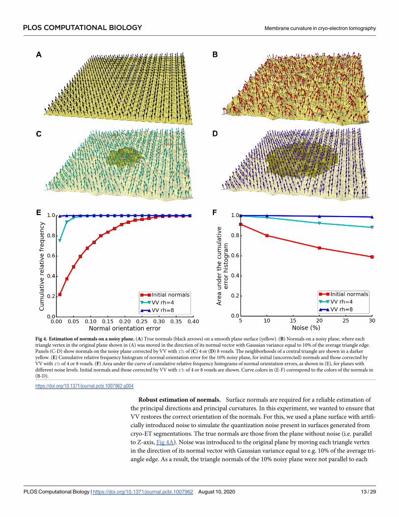
Fig 4. Estimation of normals on a noisy plane. (A) True normals (black arrows) on a smooth plane surface (yellow). (B) Normals on a noisy plane, where each

triangle vertex in the original plane shown in (A) was moved in the direction of its normal vector with Gaussian variance equal to 10% of the average triangle edge.

Panels (C-D) show normals on the noisy plane corrected by VV with rh of (C) 4 or (D) 8 voxels. The neighborhoods of a central triangle are shown in a darker

yellow. (E) Cumulative relative frequency histogram of normal orientation error for the 10% noisy plane, for initial (uncorrected) normals and those corrected by

VV with rh of 4 or 8 voxels. (F) Area under the curve of cumulative relative frequency histograms of normal orientation errors, as shown in (E), for planes with

different noise levels. Initial normals and those corrected by VV with rh of 4 or 8 voxels are shown. Curve colors in (E-F) correspond to the colors of the normals in

(B-D).






other nor to Z-axis (Fig 4B), which was also reflected by the normal orientation errors up to

�30% (Fig 4E). Using VV with rh of 4 voxels, the original orientation of the normals was

almost restored (Fig 4C), and the errors reduced to below 10% (Fig 4E). Using rh of 8 voxels,

the estimation further improved (Fig 4D and 4E), since more neighboring triangles helped to

average out the noise. For planes with more noise, the normal orientation errors of the initial

normals and the estimated ones with rh of 4 voxels increased, reducing the area under the

histogram curve. However, the estimation stayed robust using rh of 8 voxels even for a 30%

noisy plane (Fig 4F). Thus, using VV with a high enough rh substantially restores the original

orientation of the normals.

Setting the neighborhood parameter. As shown above, the size of the neighborhood

defined by the rh parameter influences the estimation of normals. Therefore, choosing an

appropriate rh for the data is crucial for accurate curvature estimation.

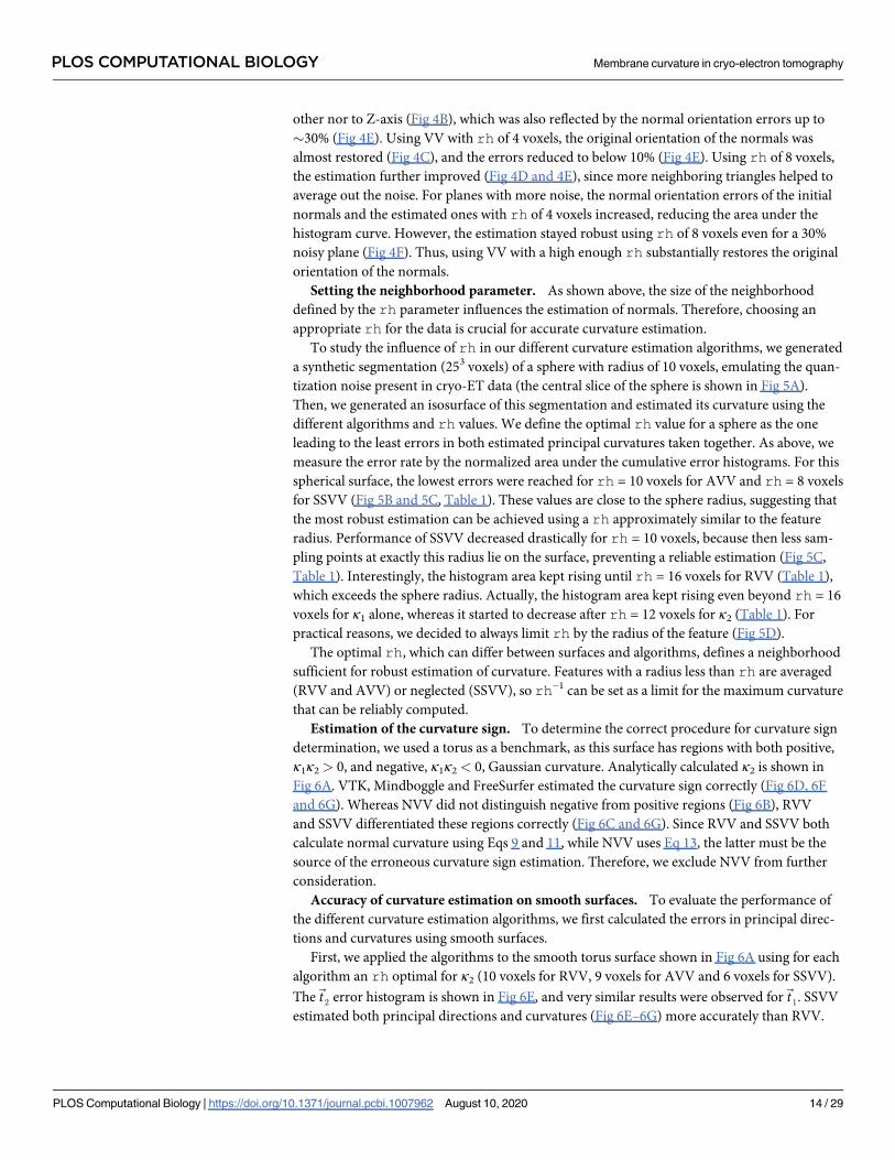
To study the influence of rh in our different curvature estimation algorithms, we generated

a synthetic segmentation (253 voxels) of a sphere with radius of 10 voxels, emulating the quan-

tization noise present in cryo-ET data (the central slice of the sphere is shown in Fig 5A).

Then, we generated an isosurface of this segmentation and estimated its curvature using the

different algorithms and rh values. We define the optimal rh value for a sphere as the one

leading to the least errors in both estimated principal curvatures taken together. As above, we

measure the error rate by the normalized area under the cumulative error histograms. For this

spherical surface, the lowest errors were reached for rh = 10 voxels for AVV and rh = 8 voxels

for SSVV (Fig 5B and 5C, Table 1). These values are close to the sphere radius, suggesting that

the most robust estimation can be achieved using a rh approximately similar to the feature

radius. Performance of SSVV decreased drastically for rh = 10 voxels, because then less sam-

pling points at exactly this radius lie on the surface, preventing a reliable estimation (Fig 5C,

Table 1). Interestingly, the histogram area kept rising until rh = 16 voxels for RVV (Table 1),

which exceeds the sphere radius. Actually, the histogram area kept rising even beyond rh = 16

voxels for κ1 alone, whereas it started to decrease after rh = 12 voxels for κ2 (Table 1). For

practical reasons, we decided to always limit rh by the radius of the feature (Fig 5D).

The optimal rh, which can differ between surfaces and algorithms, defines a neighborhood

sufficient for robust estimation of curvature. Features with a radius less than rh are averaged

(RVV and AVV) or neglected (SSVV), so rh−1 can be set as a limit for the maximum curvature

that can be reliably computed.

Estimation of the curvature sign. To determine the correct procedure for curvature sign

determination, we used a torus as a benchmark, as this surface has regions with both positive,

κ1κ2 > 0, and negative, κ1κ2 < 0, Gaussian curvature. Analytically calculated κ2 is shown in

Fig 6A. VTK, Mindboggle and FreeSurfer estimated the curvature sign correctly (Fig 6D, 6F

and 6G). Whereas NVV did not distinguish negative from positive regions (Fig 6B), RVV

and SSVV differentiated these regions correctly (Fig 6C and 6G). Since RVV and SSVV both

calculate normal curvature using Eqs 9 and 11, while NVV uses Eq 13, the latter must be the

source of the erroneous curvature sign estimation. Therefore, we exclude NVV from further

consideration.

Accuracy of curvature estimation on smooth surfaces. To evaluate the performance of

the different curvature estimation algorithms, we first calculated the errors in principal direc-

tions and curvatures using smooth surfaces.

First, we applied the algorithms to the smooth torus surface shown in Fig 6A using for each

algorithm an rh optimal for κ2 (10 voxels for RVV, 9 voxels for AVV and 6 voxels for SSVV).

The~t2 error histogram is shown in Fig 6E, and very similar results were observed for~t1. SSVV

estimated both principal directions and curvatures (Fig 6E–6G) more accurately than RVV.




AVV slightly outperformed RVV in the estimation of principal curvatures. However, VTK

estimated principal curvatures slightly better than the tensor voting-based algorithms for this

smooth surface with uniform triangles. Mindboggle with the optimal (for κ2) n = 4 voxels was

the best method for estimating κ1 (Fig 6F), but the worst for κ2 (Fig 6D and 6G), whereas Free-

Surfer performed the best for κ2 (Fig 6G). Note that the curvature errors for κ1 (Fig 6F) were

lower than for κ2 (Fig 6G) for all algorithms. A possible explanation is that κ1 is constant for a

torus and thus easier to estimate, while κ2 changes depending on the position.

We also compared the algorithms using a smooth spherical surface with a non-uniform tri-

angle tessellation, generated from a spherical volume mask smoothed using a 3D Gaussian

function (σ = 3.3) and applying an isosurface. Since both principal curvatures should be the

same for a spherical surface, they were considered together. Also, no true principal directions

exist for a spherical surface. For a sphere with radius = 10 voxels, the optimal values of rh

Fig 5. rh parameter choice. (A) A central slice of a synthetic segmentation of a sphere with radius = 10 voxels. Panels (B-D) show cumulative frequency

histograms of the κ1 and κ2 errors on the surface extracted from the segmentation shown in (A), using different rh (5-10 voxels) and algorithms: (B) AVV, (C)

SSVV and (D) RVV.






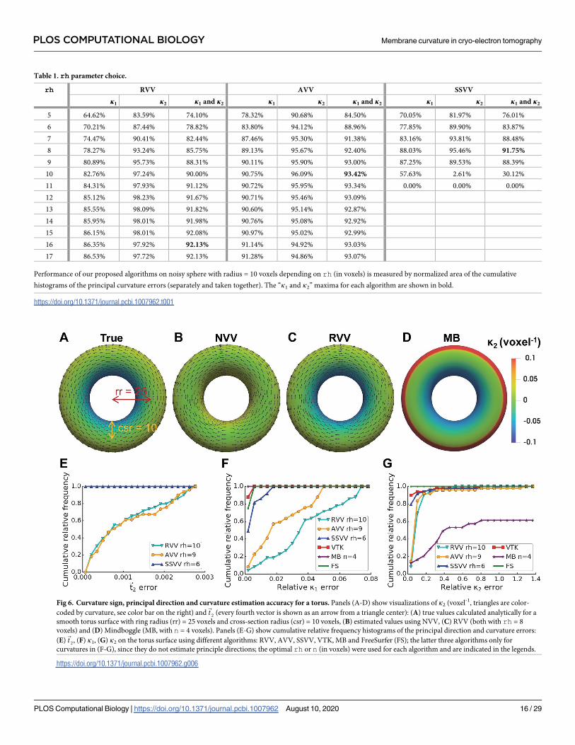
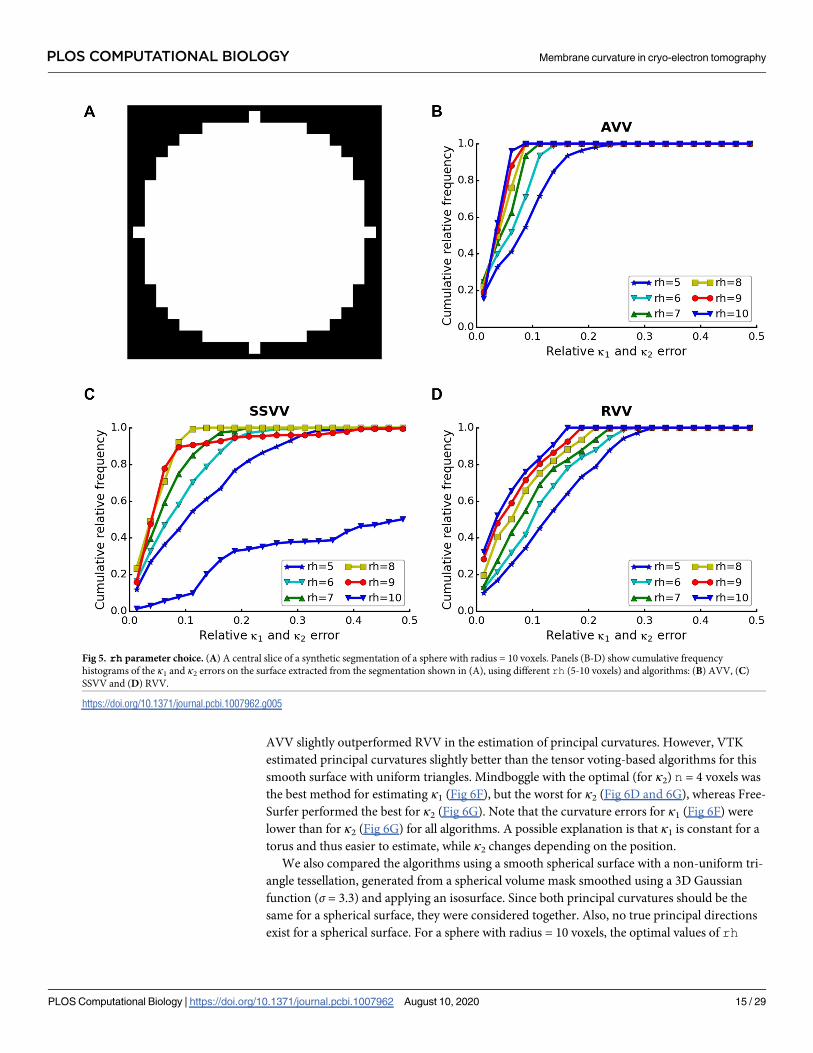
Table 1. rh parameter choice.

rh RVV AVV SSVV

κ1 κ2 κ1 and κ2 κ1 κ2 κ1 and κ2 κ1 κ2 κ1 and κ2

5 64.62% 83.59% 74.10% 78.32% 90.68% 84.50% 70.05% 81.97% 76.01%

6 70.21% 87.44% 78.82% 83.80% 94.12% 88.96% 77.85% 89.90% 83.87%

7 74.47% 90.41% 82.44% 87.46% 95.30% 91.38% 83.16% 93.81% 88.48%

8 78.27% 93.24% 85.75% 89.13% 95.67% 92.40% 88.03% 95.46% 91.75%

9 80.89% 95.73% 88.31% 90.11% 95.90% 93.00% 87.25% 89.53% 88.39%

10 82.76% 97.24% 90.00% 90.75% 96.09% 93.42% 57.63% 2.61% 30.12%

11 84.31% 97.93% 91.12% 90.72% 95.95% 93.34% 0.00% 0.00% 0.00%

12 85.12% 98.23% 91.67% 90.71% 95.46% 93.09%

13 85.55% 98.09% 91.82% 90.60% 95.14% 92.87%

14 85.95% 98.01% 91.98% 90.76% 95.08% 92.92%

15 86.15% 98.01% 92.08% 90.97% 95.02% 92.99%

16 86.35% 97.92% 92.13% 91.14% 94.92% 93.03%

17 86.53% 97.72% 92.13% 91.28% 94.86% 93.07%

Performance of our proposed algorithms on noisy sphere with radius = 10 voxels depending on rh (in voxels) is measured by normalized area of the cumulative

histograms of the principal curvature errors (separately and taken together). The “κ1 and κ2” maxima for each algorithm are shown in bold.

https://doi.org/10.1371/journal.pcbi.1007962.t001

Fig 6. Curvature sign, principal direction and curvature estimation accuracy for a torus. Panels (A-D) show visualizations of κ2 (voxel-1, triangles are color-

coded by curvature, see color bar on the right) and~t2 (every fourth vector is shown as an arrow from a triangle center): (A) true values calculated analytically for a

smooth torus surface with ring radius (rr) = 25 voxels and cross-section radius (csr) = 10 voxels, (B) estimated values using NVV, (C) RVV (both with rh = 8

voxels) and (D) Mindboggle (MB, with n = 4 voxels). Panels (E-G) show cumulative relative frequency histograms of the principal direction and curvature errors:

(E)~t2, (F) κ1, (G) κ2 on the torus surface using different algorithms: RVV, AVV, SSVV, VTK, MB and FreeSurfer (FS); the latter three algorithms only for

curvatures in (F-G), since they do not estimate principle directions; the optimal rh or n (in voxels) were used for each algorithm and are indicated in the legends.




https://doi.org/10.1371/journal.pcbi.1007962.t001



were used: 10 voxels for RVV and AVV and 9 voxels for SSVV as well as the optimal n = 2 vox-

els for Mindboggle. VTK, Mindboggle and FreeSurfer had very high errors (Fig 7A, 7B and

7E). The maximum error was only�0.16 for RVV (Fig 7C and 7E), while AVV achieved a

substantial improvement (maximum error�0.03) over RVV (Fig 7D and 7E), presumably

because of the non-uniform tessellation of the sphere. SSVV performed slightly better than

AVV (maximum error�0.01; Fig 7E).

To test how stable the algorithms are for different curvature scales, we increased the radius

of the smooth sphere from 10 to 20 voxels, while leaving the rh and n values the same. All

algorithms performed almost the same as for the sphere with radius 10 voxels (Fig 7F).

Altogether, the evaluation results on smooth benchmark surfaces show that the tensor vot-

ing-based algorithms are quite stable to feature sizes variations (beyond rh) and irregular tri-

angles within one surface (Fig 7), whereas VTK, Mindboggle and FreeSurfer only perform well

for a very smooth surface with a regular triangulation (Fig 6). AVV can deal with non-uni-

formly tessellated surfaces better than RVV, likely because curvature votes are also weighted

by relative triangle area in AVV. In the original algorithm [33], weighting curvature votes by

triangle area would not make sense because normals and curvatures are estimated at triangle

vertices. Since we decided to estimate normals and curvatures at triangle centers instead, cur-

vature votes are cast by complete triangles and weighting them by triangle area proved to be

advantageous.

Fig 7. Accuracy of curvature estimation on a smooth spherical surface. Panels (A-D) show visualizations of κ2 (voxel-1) estimated by (A) VTK, (B) FreeSurfer

(FS), (C) RVV or (D) AVV on a smooth sphere with radius = 10 voxels, using rh = 10 voxels for RVV and AVV. Panels (E-F) show cumulative relative frequency

histograms of the principal curvature (κ1 and κ2) errors on a smooth sphere with radius = 10 (E) or 20 voxels (F) using different algorithms: RVV, AVV, SSVV,

VTK, Mindboggle (MB) and FS; the values of rh or n (in voxels) used for each algorithm are indicated in the legends.






Robustness to surface noise. Surfaces generated from segmentations of biological mem-

branes are not smooth, as the surface triangles tend to follow the voxel boundaries resulting in

steps. As we are considering binary voxel values, the size of the steps depends on the voxel size

of the segmented tomogram.

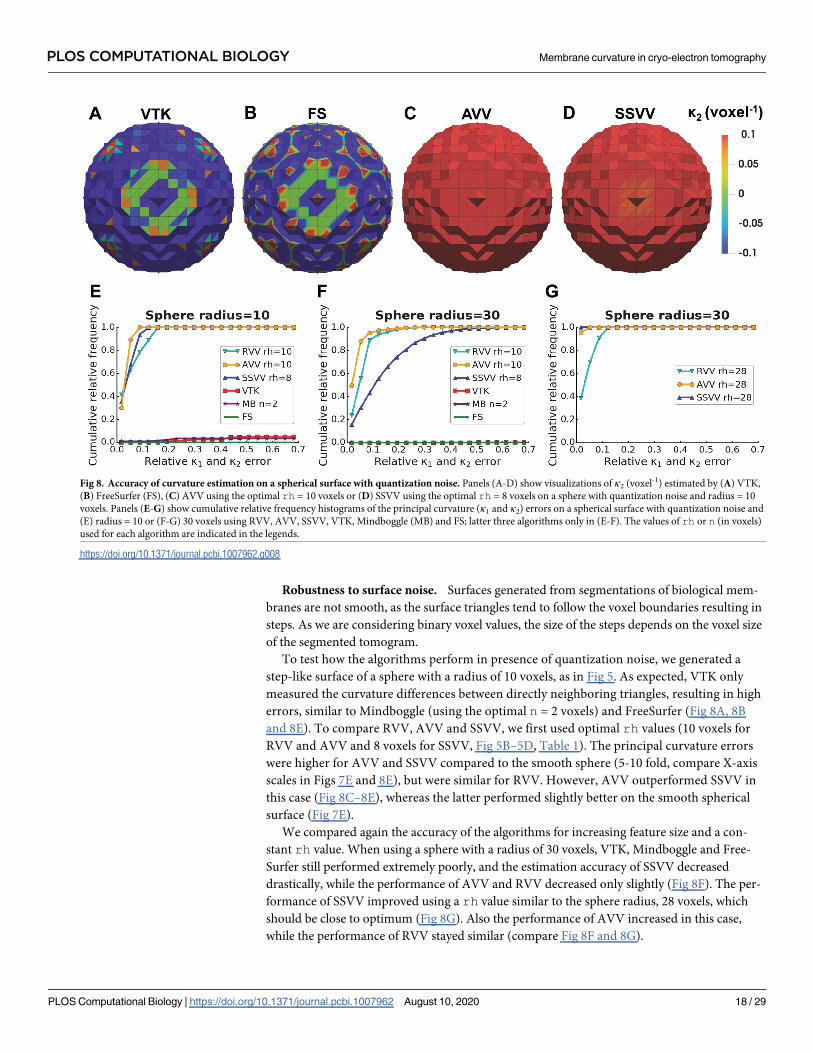
To test how the algorithms perform in presence of quantization noise, we generated a

step-like surface of a sphere with a radius of 10 voxels, as in Fig 5. As expected, VTK only

measured the curvature differences between directly neighboring triangles, resulting in high

errors, similar to Mindboggle (using the optimal n = 2 voxels) and FreeSurfer (Fig 8A, 8B

and 8E). To compare RVV, AVV and SSVV, we first used optimal rh values (10 voxels for

RVV and AVV and 8 voxels for SSVV, Fig 5B–5D, Table 1). The principal curvature errors

were higher for AVV and SSVV compared to the smooth sphere (5-10 fold, compare X-axis

scales in Figs 7E and 8E), but were similar for RVV. However, AVV outperformed SSVV in

this case (Fig 8C–8E), whereas the latter performed slightly better on the smooth spherical

surface (Fig 7E).

We compared again the accuracy of the algorithms for increasing feature size and a con-

stant rh value. When using a sphere with a radius of 30 voxels, VTK, Mindboggle and Free-

Surfer still performed extremely poorly, and the estimation accuracy of SSVV decreased

drastically, while the performance of AVV and RVV decreased only slightly (Fig 8F). The per-

formance of SSVV improved using a rh value similar to the sphere radius, 28 voxels, which

should be close to optimum (Fig 8G). Also the performance of AVV increased in this case,

while the performance of RVV stayed similar (compare Fig 8F and 8G).

Fig 8. Accuracy of curvature estimation on a spherical surface with quantization noise. Panels (A-D) show visualizations of κ2 (voxel-1) estimated by (A) VTK,

(B) FreeSurfer (FS), (C) AVV using the optimal rh = 10 voxels or (D) SSVV using the optimal rh = 8 voxels on a sphere with quantization noise and radius = 10

voxels. Panels (E-G) show cumulative relative frequency histograms of the principal curvature (κ1 and κ2) errors on a spherical surface with quantization noise and

(E) radius = 10 or (F-G) 30 voxels using RVV, AVV, SSVV, VTK, Mindboggle (MB) and FS; latter three algorithms only in (E-F). The values of rh or n (in voxels)

used for each algorithm are indicated in the legends.






Therefore, when quantization noise is present, all our algorithms perform better than

the currently available methods tested here. SSVV requires a higher rh in the range of the cur-

vature radius, while AVV is quite stable with a lower rh value. Using a very high rh is gener-

ally not advisable, as it would lead to the underestimation of curvatures at smaller surface

features. Since RVV performed consistently worse than AVV, we exclude RVV from further

comparison.

Higher errors at surface borders. As explained previously, membranes in cryo-ET seg-

mentations have holes and open ends. Thus, we aimed for a curvature estimation algorithm

that is robust to such artifacts.

Tensor voting-based algorithms use a supporting neighborhood in order to improve the

estimation, so holes much smaller than the neighborhood region do not affect them critically.

However, a vertex close to surface border has considerably less neighbors. Therefore, we

hypothesized that the estimation accuracy at vertices close to such borders would be worse. To

prove this hypothesis, we generated a smooth cylindrical surface opened at both sides with

radius = 10 and height = 25 voxels and evaluated the performance of our algorithms. Optimal

rh values were used for AVV (5 voxels) and for SSVV (6 voxels), as well as optimal n for

Mindboggle (2 voxels). FreeSurfer was not included in this test, since it failed on this open

surface.

As expected, both tensor voting-based algorithms made a worse estimation near borders:

AVV overestimated κ1 gradually when moving towards the borders and κ2 at the last triangles

(Fig 9A), while SSVV underestimated κ1 consistently and made a gradient of wrong estima-

tions for κ2 in the same region (Fig 9B). Since VTK does not use a bigger neighborhood, it

showed high errors at changes in the triangle pattern all over the cylinder (Fig 9C). Mindbog-

gle showed high errors for κ1 in a striped pattern and for κ2 at some patches near the borders

(Fig 9D). SSVV and AVV showed~t2 and κ1 errors in the same range (Fig 9E and 9F), while

VTK and Mindboggle made higher κ1 errors than our algorithms (Fig 9F). When excluding

values within the distance of 5 voxels to the graph border, the errors were virtually eliminated

for AVV and SSVV, but did not change for VTK (Fig 9G and 9H). For Mindboggle, we could

not exclude values at borders because our graph structure used for borders filtering is not

available for that method. However, as one can see in Fig 9D, the high κ1 errors of Mindboggle

would not have been eliminated with this strategy.

Altogether, these benchmark results demonstrate the validity of our tensor voting-based

algorithms and their robustness to quantization noise, especially of AVV. Additionally, curva-

ture estimations at surface borders can be erroneous, so they should be excluded from an

analysis.

Application to biological surfaces

Choice of algorithms and parameters for membranes from cryo-ET. AVV and SSVV

proved most robust to quantization noise in synthetic surfaces. To evaluate their performance

on real cryo-ET data, we used a cER compartment segmentation that contains several high

curvature regions or peaks [16].

First, we studied the relationship between the rh parameter and the feature size. For this,

we isolated a single cER peak with a maximum base radius of approximately 10 nm from a

tomogram and estimated its curvature using several rh values. We observed that real mem-

brane features have a diverse curvature distribution with several local maxima and minima

(Fig 10A and 10B). For low values of rh, the distributions of curvature are broad, getting pro-

gressively sharper with increasing rh. For AVV (Fig 10A), the maximum amount of values

around 0.1 nm-1 (corresponding to the 10 nm radius of the peak) is reached for rh = 10,




Fig 9. Estimation accuracy on a cylindrical surface. Panels (A-D) show principal curvatures on a smooth cylinder with radius = 10 and height = 25

voxels estimated by different algorithms: (A) AVV using the optimal rh = 5 voxels, (B) SSVV using the optimal rh = 6 voxels, (C) VTK and (D)

Mindboggle (MB) using the optimal n = 2 voxels; the estimated κ1 and κ2 are shown in their original ranges; true κ1 = 0.1, true κ2 = 0 voxel-1. Panels

(E-H) show cumulative relative frequency histograms of the~t2 errors (E, G) and κ1 errors (F, H) on the cylinder using different algorithms: AVV,

SSVV, VTK and MB; latter two algorithms only for κ1 in (F, H); the optimal rh or n (in voxels) were used for each algorithm and are indicated in the

legends. In panels (G-H), values within 5 voxels to the graph border were excluded.






indicating that the feature is observed as a whole and its smaller components fade. Higher rhno longer produce curvature values around 0.1 nm-1, indicating that the feature is averaged

out. A similar trend is observed for SSVV (Fig 10B), although this method produces less curva-

ture values around 0.1 nm-1, thus underestimating the real curvature of the feature.

Second, we visualized the principal curvatures of the feature using rh = 10 nm to analyze

the difference between the two curvature estimation algorithms. For this specific feature, its

principal curvatures estimated by AVV (Fig 10C) increased in the direction from the base to

the summit, while SSVV (Fig 10D) underestimated the curvatures, especially κ2. Since SSVV

sampled only surface points at distance equal to rh of 10 nm from each triangle center, it

“oversaw” the high curvature at and near the summit. Contrary to SSVV, AVV considered all

triangles within the geodesic neighborhood and thus estimated the curvature increase towards

the summit correctly. This example confirms that AVV performs better than SSVV for com-

plex surfaces like biological membranes.

Lastly, we applied AVV with rh = 10 nm to the full cER membrane surface, from which the

peak shown in Fig 10 was extracted (Fig 11A and 11B). For comparison, we also applied VTK

and Mindboggle to this surface (Fig 11C). Visually, n = 2 nm yielded the best results for Mind-

boggle. On this membrane surface, AVV clearly outperforms VTK and Mindboggle, which

Fig 10. Algorithms and parameters comparison using a small cER membrane feature from cryo-ET. Surface of a cER membrane region with maximum base

radius�10 nm (from the same tomogram of a yeast cell as the cER in Fig 11) was generated using the compartment segmentation. Panels (A-B) show relative

frequency histograms of κ1 estimated by (A) AVV or (B) SSVV using rh = 2, 5, 10, 15 and 20 nm. Panels (C-D) show visualizations of the estimated κ1 and κ2 (color

scale was set to the value range of [-0.1, 0.1] nm-1 in both panels) and the corresponding principal directions (black arrows, sampled for every forth triangle) by (C)

AVV or (D) SSVV using rh = 10 nm (scale bar: 20 nm, applies for both panels).






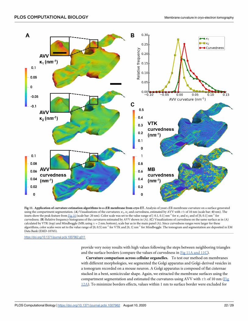
provide very noisy results with high values following the steps between neighboring triangles

and the surface borders (compare the values of curvedness in Fig 11A and 11C).

Curvature comparison across cellular organelles. To test our method on membranes

with different morphologies, we segmented the Golgi apparatus and Golgi-derived vesicles in

a tomogram recorded on a mouse neuron. A Golgi apparatus is composed of flat cisternae

stacked in a bent, semicircular shape. Again, we extracted the membrane surfaces using the

compartment segmentation and estimated the curvatures using AVV with rh of 10 nm (Fig

12A). To minimize borders effects, values within 1 nm to surface border were excluded for

Fig 11. Application of curvature estimation algorithms to a cER membrane from cryo-ET. Analysis of yeast cER membrane curvature on a surface generated

using the compartment segmentation. (A) Visualizations of the curvatures: κ1, κ2 and curvedness, estimated by AVV with rh of 10 nm (scale bar: 40 nm). The

insets show the peak feature from Fig 10 (scale bar: 20 nm). Color scale was set to the value range of [-0.1, 0.1] nm-1 for κ1 and κ2 and of [0, 0.1] nm-1 for

curvedness. (B) Relative frequency histograms of the curvatures estimated by AVV shown in (A). (C) Visualizations of curvedness on the same surface as in (A)

calculated by VTK (top) and Mindboggle (MB; using n = 2 nm; bottom), scale bar as in the main panel (A). Since curvedness ranges were larger for these

algorithms, color scales were set to the value range of [0, 0.5] nm-1 for VTK and [0, 1] nm-1 for Mindboggle. The tomogram and segmentation are deposited in EM

Data Bank (EMD-10765).






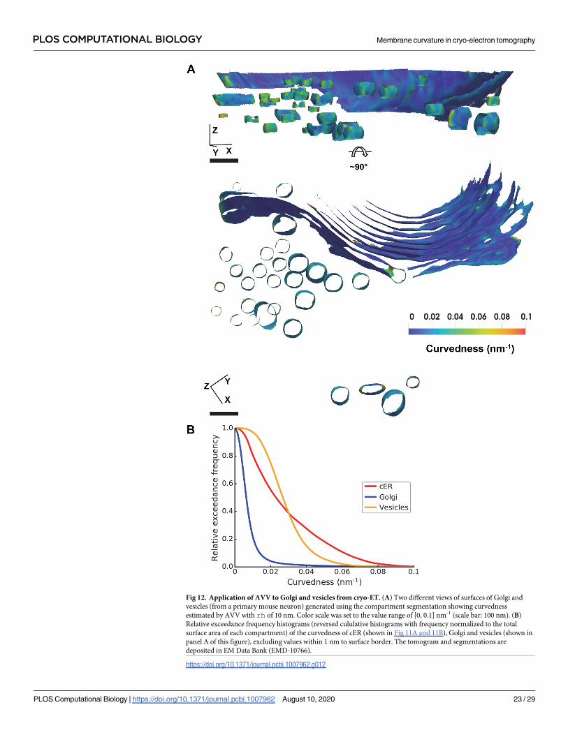
Fig 12. Application of AVV to Golgi and vesicles from cryo-ET. (A) Two different views of surfaces of Golgi and

vesicles (from a primary mouse neuron) generated using the compartment segmentation showing curvedness

estimated by AVV with rh of 10 nm. Color scale was set to the value range of [0, 0.1] nm-1 (scale bar: 100 nm). (B)

Relative exceedance frequency histograms (reversed cululative histograms with frequency normalized to the total

surface area of each compartment) of the curvedness of cER (shown in Fig 11A and 11B), Golgi and vesicles (shown in

panel A of this figure), excluding values within 1 nm to surface border. The tomogram and segmentations are

deposited in EM Data Bank (EMD-10766).






plotting. Fig 12B compares the curvedness of the cER (Fig 11) with that of the Golgi and

Golgi-derived vesicles. The histogram shows that the Golgi has much lower curvedness than

the other two organelles, whereas the cER reaches higher curvedness values than the vesicles.

The results can be visually confirmed: the thin and long Golgi cisternae are only slightly

curved, while the vesicles are smaller and thus much more curved (Fig 12A). The cER is gener-

ally less curved than the vesicles, but has high curvature at the peaks and sides of its sheets (Fig

11A). These data show that curvedness estimated by AVV can be a useful descriptor of biologi-

cal membranes.

Application to other data types. To demonstrate the applicability of AVV beyond cryo-

ET, we applied it to two other data types. The first data set is comprised of C. elegans embryo

cells imaged by confocal light microscopy and segmented by LimeSeg [22]. The cell surfaces

colored by their Gaussian curvature estimated by AVV using rh = 3 μm are shown in Fig 13A.

The second data set, taken from Mindboggle [42], are cortical pial surfaces of both human

brain hemispheres imaged by MRI and segmented by FreeSurfer [52]. The cortical surfaces

colored by their mean curvature estimated by AVV using rh = 2 mm are shown in Fig 13B.

Fig 13. Application of curvature estimation algorithms to other data types. (A) Surfaces of C. elegans embryo cells imaged by confocal light microscopy and

segmented by LimeSeg [22], colored by Gaussian curvature (μm-2) estimated by AVV using rh = 3 μm (scale bar: 5 μm). (B) Cortical pial surfaces of both human

brain hemispheres imaged by MRI and segmented by FreeSurfer [52], colored by mean curvature (mm-1) estimated by AVV using rh = 2 mm (scale bar: 20 mm).

Panels (C-D) show the same brain surface colored by mean curvature (mm-1) with the same color scale as in (B) estimated by (C) Mindboggle (MB; using n = 2

mm) and (D) FreeSurfer (FS).






The range of curvature values for the embryo and the brain is consistent with their sizes. Using

Mindboggle [42] with n = 2 mm (Fig 13C) and FreeSurfer [41] (Fig 13D), we obtained compa-

rable, but noisier, mean curvature distributions on the brain; FreeSurfer introduced finer-

grained noise than Mindboggle. Despite the lack of ground truth, this comparison suggests

that AVV provides a more accurate curvature estimation for different data types.

Implementation and availability

All the described algorithms and the tests on benchmark surfaces were implemented using

Python and are available in PyCurv at https://github.com/kalemaria/pycurv, along with the

experimental data sets and scripts allowing to obtain the results presented in the Section Appli-

cation to biological surfaces. PyCurv depends only on open source packages, including: Pyto

[53], Graph-tool [48] and VTK [30]. Note that FreeSurfer [52] and Mindboggle [42] had to be

installed and called externally for the evaluation; FreeSurfer version “stable v6.0.0” for Linux

and Mindboggle Docker container from 2019-09-24 were used.

Discussion

In this article, we described a method for the estimation of the local curvature of biological

membranes and validated it on synthetic and real data. The curvature estimation workflow

in PyCurv can be divided in two main steps. The first step is to represent the membrane as a

triangle mesh surface that can be obtained from two different types of segmentation: segmen-

tation of the membrane alone, or a filled segmentation of a membrane-bound cellular com-

partment. The second option usually demands more human intervention but the surface

orientation could be recovered perfectly in our experiments. Smoothing of the filled segmenta-

tion prior to surface extraction leads to less quantization noise because the surface is extracted

at subvoxel precision. Surface triangles are mapped to a graph to facilitate the computation of

geodesic distances and to filter border artifacts. The second step is to determine the underlying

surface orientation (represented by normal vectors), local curvatures and principal directions.

Here, we evaluated the performance of our curvature estimation algorithms, RVV, AVV

and SSVV (adaptations of [33] and [40]) against the publicly available VTK [30], FreeSurfer

[41] and Mindboggle [42]. Although we chose the optimal radius of the neighborhood (n)

parameter for each benchmark surface, Mindboggle performed poorly on irregular and noisy

surfaces. Also FreeSurfer, which performed the best on a smooth and regular surface, yielded

high errors on irregular and noisy surfaces. Moreover, FreeSurfer cannot be applied to surfaces

containing borders, so it is not applicable for cryo-ET data. Our tests using synthetic and bio-

logical surfaces showed that the proposed algorithms, RVV, AVV and SSVV, are more robust

to quantization noise than the above-mentioned existing methods. AVV performs better than

RVV for non-uniformly tessellated surfaces. For complex non-spherical surfaces like biological

membranes, AVV yields better results than SSVV. Therefore, AVV is the default algorithm in

PyCurv.

Curvature is a local property, so its value on discrete surfaces depends on the definition of a

neighborhood. Robustness to noise increases with the neighborhood size by averaging the con-

tributions of the neighboring triangles. However, features smaller than the neighborhood are

averaged out. Therefore, the neighborhood size defines the scale of the features that can be

analyzed. To achieve more reliable results for cryo-ET segmentations that contain holes, curva-

ture values at surface borders and/or higher than rh-1 should be excluded from the analysis.

PyCurv was already applied in a cryo-ET study in yeast proposing that cER membrane cur-

vature plays a key role in the regulation of ER-to-PM lipid homeostasis at membrane contact

sites [16]. Moreover, the analysis of data generated by MRI and light microscopy shows that




https://github.com/vladanl/Pyto

https://graph-tool.skewed.de

https://vtk.org

https://surfer.nmr.mgh.harvard.edu

https://github.com/nipy/mindboggle


our method can be applied to any segmented membrane compartments or other volumes

from which a surface can be extracted, originating from any 3D imaging technique. We con-

clude that the open-source Python package PyCurv can be used to reliably process cryo-ET

and other data to study membrane and surface curvature in a large variety of applications.

Supporting information

S1 Video. PyCurv workflow. The visualization of PyCurv processing workflow, as described

in Fig 1A, for the tomogram from Fig 2, showing in the order of occurrence: membrane and

compartment segmentations of the cortical ER, generated surface, normals estimated by Vector

Voting (VV) and curvedness estimated by Augmented Vector Voting (AVV) algorithms.

(MP4)

Acknowledgments

We thank Markus Hohle, Vladan Lučić and Martin Salfer for helpful discussions as well as

Felix J.B. Bauerlein and Tillman Schafer for tomography data.

Author Contributions

Conceptualization: Maria Salfer, Wolfgang Baumeister, Ruben Fernandez-Busnadiego, Anto-

nio Martınez-Sanchez.

Data curation: Maria Salfer, Javier F. Collado.

Formal analysis: Antonio Martınez-Sanchez.

Funding acquisition: Maria Salfer, Javier F. Collado, Wolfgang Baumeister, Ruben Fernan-

dez-Busnadiego.

Investigation: Maria Salfer, Javier F. Collado.

Methodology: Ruben Fernandez-Busnadiego, Antonio Martınez-Sanchez.

Project administration: Wolfgang Baumeister, Ruben Fernandez-Busnadiego.

Resources: Wolfgang Baumeister.

Software: Maria Salfer.

Supervision: Ruben Fernandez-Busnadiego, Antonio Martınez-Sanchez.

Validation: Maria Salfer, Ruben Fernandez-Busnadiego, Antonio Martınez-Sanchez.

Visualization: Maria Salfer, Ruben Fernandez-Busnadiego, Antonio Martınez-Sanchez.

Writing – original draft: Maria Salfer, Ruben Fernandez-Busnadiego, Antonio Martınez-

Sanchez.

Writing – review & editing: Maria Salfer, Ruben Fernandez-Busnadiego, Antonio Martınez-

Sanchez.

References1. McMahon HT, Boucrot E. Membrane curvature at a glance. J Cell Sci. 2015; 128(6):1065–1070. https://

doi.org/10.1242/jcs.114454 PMID: 25774051

2. Bassereau P, Jin R, Baumgart T, Deserno M, Dimova R, Frolov VA, et al. The 2018 biomembrane cur-

vature and remodeling roadmap. J Phys D Appl Phys. 2018; 51(34). https://doi.org/10.1088/1361-6463/

aacb98 PMID: 30655651



http://journals.plos.org/ploscompbiol/article/asset?unique&id=info:doi/10.1371/journal.pcbi.1007962.s001

https://doi.org/10.1242/jcs.114454

https://doi.org/10.1242/jcs.114454

http://www.ncbi.nlm.nih.gov/pubmed/25774051

https://doi.org/10.1088/1361-6463/aacb98

https://doi.org/10.1088/1361-6463/aacb98



3. Kozlov MM, Campelo F, Liska N, Chernomordik LV, Marrink SJ, McMahon HT. Mechanisms shaping

cell membranes. Curr Opin Cell Biol. 2014; 29:53–60. https://doi.org/10.1016/j.ceb.2014.03.006 PMID:

24747171

4. Lučić V, Forster F, Baumeister W. Structural Studies By Electron Tomography: From Cells to Mole-

cules. Annu Rev Biochem. 2005; 74:833–865. https://doi.org/10.1146/annurev.biochem.73.011303.

074112 PMID: 15952904

5. Beck M, Baumeister W. Cryo-Electron Tomography: Can it Reveal the Molecular Sociology of Cells in

Atomic Detail? Trends Cell Biol. 2016; 26(11):825–837. https://doi.org/10.1016/j.tcb.2016.08.006

PMID: 27671779

6. Wagner J, Schaffer M, Fernandez-Busnadiego R. Cryo-electron tomography—the cell biology that

came in from the cold. FEBS Lett. 2017; 591:2520–2533. https://doi.org/10.1002/1873-3468.12757

PMID: 28726246

7. Collado J, Fernandez-Busnadiego R. Deciphering the molecular architecture of membrane contact

sites by cryo-electron tomography. Biochim Biophys Acta Mol Cell Res. 2017; 1864:1507–1512. https://

doi.org/10.1016/j.bbamcr.2017.03.009 PMID: 28330771

8. O’Reilly FJ, Xue L, Graziadei A, Sinn L, Lenz S, Tegunov D, et al. In-cell architecture of an actively tran-

scribing-translating expressome. Science 2020; 369(6503):554–557. https://doi.org/10.1126/science.

abb3758 PMID: 32732422

9. Chen Y, Yong J, Martınez-Sanchez A, Yang Y, Wu Y, De Camilli P, et al. Dynamic instability of clathrin

assembly provides proofreading control for endocytosis. J Cell Biol. 2019; 218(10):3200–3211. https://

doi.org/10.1083/jcb.201804136 PMID: 31451612

10. Lee KK. Architecture of a nascent viral fusion pore. EMBO J. 2010; 29(7):1299–1311. https://doi.org/10.

1038/emboj.2010.13 PMID: 20168302

11. Cardone G, Brecher M, Fontana J, Winkler DC, Butan C, White JM, et al. Visualization of the Two-Step

Fusion Process of the Retrovirus Avian Sarcoma/Leukosis Virus by Cryo-Electron Tomography. J Virol.

2012; 86(22):12129–12137. https://doi.org/10.1128/JVI.01880-12 PMID: 22933285

12. Bharat TAM, Malsam J, Hagen WJH, Scheutzow A, Sollner TH, Briggs JAG. SNARE and regulatory

proteins induce local membrane protrusions to prime docked vesicles for fast calcium-triggered fusion.

EMBO Rep. 2014; 15(3):308–314. https://doi.org/10.1002/embr.201337807 PMID: 24493260

13. Chlanda P, Mekhedov E, Waters H, Schwartz CL, Fischer ER, Ryham RJ, et al. The hemifusion struc-

ture induced by influenza virus haemagglutinin is determined by physical properties of the target mem-

branes. Nat Microbiol. 2016; 1(6):1–8. https://doi.org/10.1038/nmicrobiol.2016.50 PMID: 27572837

14. Yao Q, Jewett AI, Chang YW, Oikonomou CM, Beeby M, Iancu CV, et al. Short FtsZ filaments can drive

asymmetric cell envelope constriction at the onset of bacterial cytokinesis. EMBO J. 2017; 36

(11):1577–1589. https://doi.org/10.15252/embj.201696235 PMID: 28438890

15. Bharat TAM, Hoffmann PC, Kukulski W. Correlative Microscopy of Vitreous Sections Provides Insights

into BAR-Domain Organization In Situ. Structure. 2018; 26(6):879–886. https://doi.org/10.1016/j.str.

2018.03.015 PMID: 29681471

16. Collado J, Kalemanov M, Campelo F, Bourgoint C, Thomas F, Loewith R, et al. Tricalbin-Mediated Con-

tact Sites Control ER Curvature to Maintain Plasma Membrane Integrity. Dev Cell. 2019; 51:476–487.

https://doi.org/10.1016/j.devcel.2019.10.018 PMID: 31743662

17. Bauerlein FJB, Saha I, Mishra A, Kalemanov M, Martınez-Sanchez A, Klein R, et al. In Situ Architecture

and Cellular Interactions of PolyQ Inclusions. Cell. 2017; 171:179–187. https://doi.org/10.1016/j.cell.

2017.08.009 PMID: 28890085

18. Martinez-Sanchez A, Garcia I, Asano S, Lucic V, Fernandez JJ. Robust membrane detection based on

tensor voting for electron tomography. J Struct Biol. 2014; 186:49–61. https://doi.org/10.1016/j.jsb.

2014.02.015 PMID: 24625523

19. Martinez-Sanchez A, Kochovski Z, Laugks U, Meyer zum Alten Borgloh J, Chakraborty S, Pfeffer S,

et al. Template-free detection and classification of membrane-bound complexes in cryo-electron tomo-

grams. Nat Methods. 2020; p. 1–15. https://doi.org/10.1038/s41592-019-0675-5 PMID: 31907446

20. Mosaliganti KR, Noche RR, Xiong F, Swinburne IA, Megason SG. ACME: Automated Cell Morphology

Extractor for Comprehensive Reconstruction of Cell Membranes. PLoS Comput Biol. 2012; 8(12):

e1002780. https://doi.org/10.1371/journal.pcbi.1002780 PMID: 23236265

21. Chen M, Dai W, Sun SY, Jonasch D, He CY, Schmid MF, et al. Convolutional neural networks for auto-

mated annotation of cellular cryo-electron tomograms. Nat Methods. 2017; 14(10):983–985. https://doi.

org/10.1038/nmeth.4405 PMID: 28846087

22. Machado S, Mercier V, Chiaruttini N. LimeSeg: A coarse-grained lipid membrane simulation for 3D

image segmentation. BMC Bioinformatics. 2019; 20(2):1–12. https://doi.org/10.1186/s12859-018-

2471-0 PMID: 30606118



https://doi.org/10.1016/j.ceb.2014.03.006


https://doi.org/10.1146/annurev.biochem.73.011303.074112

https://doi.org/10.1146/annurev.biochem.73.011303.074112


https://doi.org/10.1016/j.tcb.2016.08.006


https://doi.org/10.1002/1873-3468.12757


https://doi.org/10.1016/j.bbamcr.2017.03.009

https://doi.org/10.1016/j.bbamcr.2017.03.009


https://doi.org/10.1126/science.abb3758

https://doi.org/10.1126/science.abb3758


https://doi.org/10.1083/jcb.201804136

https://doi.org/10.1083/jcb.201804136


https://doi.org/10.1038/emboj.2010.13

https://doi.org/10.1038/emboj.2010.13


https://doi.org/10.1128/JVI.01880-12


https://doi.org/10.1002/embr.201337807


https://doi.org/10.1038/nmicrobiol.2016.50


https://doi.org/10.15252/embj.201696235


https://doi.org/10.1016/j.str.2018.03.015

https://doi.org/10.1016/j.str.2018.03.015


https://doi.org/10.1016/j.devcel.2019.10.018


https://doi.org/10.1016/j.cell.2017.08.009

https://doi.org/10.1016/j.cell.2017.08.009


https://doi.org/10.1016/j.jsb.2014.02.015



https://doi.org/10.1038/s41592-019-0675-5




https://doi.org/10.1038/nmeth.4405



https://doi.org/10.1186/s12859-018-2471-0

https://doi.org/10.1186/s12859-018-2471-0



23. Martinez-Sanchez A, Garcia I, Fernandez JJ. A differential structure approach to membrane segmenta-

tion in electron tomography. J Struct Biol. 2011; 175:372–383. https://doi.org/10.1016/j.jsb.2011.05.010

PMID: 21616152

24. do Carmo MP. Differential geometry of curves and surfaces. New Jersey: Prentice-Hall, Inc., Engle-

wood Cliffs; 1976.

25. Meyer M, Desbrun M, Schroder P, Barr AH. Discrete Differential-Geometry Operators for Triangulated

2-Manifolds. Springer, Berlin, Heidelberg; 2003.

26. Hoppe H, DeRose T, Duchamp T, McDonald J, Stuetzle W. Surface reconstruction from unorganized

points. In: SIGGRAPH’92 Proceedings of the 19th annual conference on Computer graphics and inter-

active techniques. New York: ACM; 1992. p. 71–78. https://doi.org/10.1145/133994.134011

27. Magid E, Soldea O, Rivlin E. A comparison of Gaussian and mean curvature estimation methods on tri-

angular meshes of range image data. Comput Vis Image Underst. 2007; 107:139–159. https://doi.org/

10.1016/j.cviu.2006.09.007

28. Polthier K, Schmies M. Straightest Geodesics on Polyhedral Surfaces. In: Mathematical Visualization.

Springer Verlag; 1998. p. 391–409.

29. Desbrun M, Meyer M, Schroder P, Barr AH. Implicit fairing of irregular meshes using diffusion and cur-

vature flow. In: SIGGRAPH’99 Proceedings of the 26th annual conference on Computer graphics and

interactive techniques. New York: ACM Press/Addison-Wesley Publishing; 1999. p. 317–324. https://

doi.org/10.1145/311535.311576

30. Schroeder W, Martin K, Lorensen B. The Visualization Toolkit ( 4th ed.). Kitware; 2006.

31. Szilvasi-Nagy M. Face-based estimations of curvatures on triangle meshes. Journal for Geometry and

Graphics. 2008; 12(1):63–73.

32. Razdan A, Bae M. Curvature estimation scheme for triangle meshes using biquadratic Bezier patches.

Comput Aided Des. 2005; 37:1481–1491. https://doi.org/10.1016/j.cad.2005.03.003

33. Page DL, Sun Y, Koschan AF, Paik J, Abidi MA. Normal Vector Voting: Crease Detection and Curvature

Estimation on Large, Noisy Meshes. Graph Models. 2002; 64:199–229. https://doi.org/10.1006/gmod.

2002.0574

34. Goldfeather J, Interrante V. A novel cubic-order algorithm for approximating principal direction vectors.

ACM Trans Graph. 2004; 23(1):45–63. https://doi.org/10.1145/966131.966134

35. Taubin G. Estimating the tensor of curvature of a surface from a polyhedral approximation. In: Proceed-

ings of IEEE International Conference on Computer Vision. Cambridge: IEEE; 1995. p. 902–907.

https://doi.org/10.1109/ICCV.1995.466840

36. Theisel H, Rossl C, Zayer R, Seidel HP. Normal based estimation of the curvature tensor for triangular

meshes. In: 12th Pacific Conference on Computer Graphics and Applications. Seoul, South Korea:

IEEE; 2004. p. 288–297. https://doi.org/10.1109/PCCGA.2004.1348359

37. Rusinkiewicz S. Estimating curvatures and their derivatives on triangle meshes. In: Proceedings of the

2nd International Symposium on 3D Data Processing, Visualization, and Transmission. Thessaloniki,

Greece: IEEE; 2004. p. 486–493. https://doi.org/10.1109/TDPVT.2004.1335277

38. Medioni G, Lee MS, Tang CK. A Computational Framework for Segmentation and Grouping. Amster-

dam: Elsevier Science B.V.; 2000.

39. Tang CK, Medioni G. Robust Estimation of Curvature Information from Noisy 3D Data for Shape

Description. In: Proceedings of the Seventh IEEE International Conference on Computer Vision. Ker-

kyra, Greece: IEEE; 1999. https://doi.org/10.1109/ICCV.1999.791252

40. Tong WS, Tang CK. Robust Estimation of Adaptive Tensors of Curvature by Tensor Voting. In: IEEE

Trans. Pattern Anal. Mach. Intell. vol. 27; 2005. p. 434–449. https://doi.org/10.1109/tpami.2005.62

PMID: 15747797

41. Pienaar R, Fischl B, Caviness V, Makris N, Grant PE. A methodology for analyzing curvature in the

developing brain from preterm to adult. Int J Imaging Syst Technol. 2008; 18:42–68. https://doi.org/10.

1002/ima.v18:1 PMID: 19936261

42. Klein A, Ghosh SS, Bao FS, Giard J, Hame Y, Stavsky E, et al. Mindboggling morphometry of human

brains. PLoS Comput Biol. 2017; 13(2):1–40. PMID: 28231282

43. Moses DA, Axel L. Quantification of the curvature and shape of the interventricular septum. Magnetic

Resonance in Medicine. 2004; 52(1):154–163. https://doi.org/10.1002/mrm.20105 PMID: 15236379

44. Bechstedt S, Lu K, Brouhard GJ. Doublecortin recognizes the longitudinal curvature of the microtubule

end and lattice. Curr Biol. 2014; 24:2366–2375. https://doi.org/10.1016/j.cub.2014.08.039 PMID:

25283777





https://doi.org/10.1145/133994.134011

https://doi.org/10.1016/j.cviu.2006.09.007

https://doi.org/10.1016/j.cviu.2006.09.007

https://doi.org/10.1145/311535.311576

https://doi.org/10.1145/311535.311576

https://doi.org/10.1016/j.cad.2005.03.003

https://doi.org/10.1006/gmod.2002.0574

https://doi.org/10.1006/gmod.2002.0574

https://doi.org/10.1145/966131.966134


https://doi.org/10.1109/PCCGA.2004.1348359

https://doi.org/10.1109/TDPVT.2004.1335277


https://doi.org/10.1109/tpami.2005.62


https://doi.org/10.1002/ima.v18:1

https://doi.org/10.1002/ima.v18:1



https://doi.org/10.1002/mrm.20105


https://doi.org/10.1016/j.cub.2014.08.039



45. Xu M, Wu Y, Shroff H, Wu M, Mani M. A scheme for 3-dimensional morphological reconstruction and

force inference in the early C. elegans embryo. PLoS One. 2018; 13(7). https://doi.org/10.1371/journal.

pone.0199151 PMID: 29990323

46. Hoffman DP, Shtengel G, Xu CS, Campbell KR, Freeman M, Wang L, et al. Correlative three-dimen-

sional super-resolution and block face electron microscopy of whole vitreously frozen cells. Science.

2020; 367(265):14. https://doi.org/10.1126/science.aaz5357 PMID: 31949053

47. Lorensen WE, Cline HE. Marching Cubes: A High Resolution 3D Surface Construction Algorithm. ACM

SIGGRAPH Comput Graph. 1987; 21(4):163–169. https://doi.org/10.1145/37401.37422

48. Peixoto TP. The graph-tool python library. Database: figshare [Internet]; 2014. Available from: http://

figshare.com/articles/graph_tool/1164194.

49. Dijkstra EW. A Note on Two Problems in Connexion with Graphs. Numer Math. 1959; 1:269–271.

50. Koenderink JJ, van Doorn AJ. Surface shape and curvature scales. Image Vis Comput. 1992; 10

(8):557–564. https://doi.org/10.1016/0262-8856(92)90076-F

51. Ahrens J, Geveci B, Law C. ParaView: An end-user tool for large-data visualization. Visualization Hand-

book. 2005; 836:717–731. https://doi.org/10.1016/B978-012387582-2%2F50038-1

52. Dale AM, Fischl B, Sereno MI. Cortical Surface-Based Analysis. Neuroimage. 1999; 9:179–194. https://

doi.org/10.1006/nimg.1998.0395 PMID: 9931268

53. Lučić V, Fernandez-Busnadiego R, Laugks U, Baumeister W. Hierarchical detection and analysis of

macromolecular complexes in cryo-electron tomograms using Pyto software. J Struct Biol. 2016; 196

(3):503–514. https://doi.org/10.1016/j.jsb.2016.10.004 PMID: 27742578

54. Rigort A, Bauerlein FJB, Villa E, Eibauer M, Laugks T, Baumeister W, et al. Focused ion beam microma-

chining of eukaryotic cells for cryoelectron tomography. PNAS. 2012; 109(12):4449–4454. https://doi.

org/10.1073/pnas.1201333109 PMID: 22392984

55. Mastronarde DN. Automated electron microscope tomography using robust prediction of specimen

movements. J Struct Biol. 2005; 152:36–51. https://doi.org/10.1016/j.jsb.2005.07.007 PMID: 16182563

56. Li X, Mooney P, Zheng S, Booth CR, Braunfeld MB, Gubbens S, et al. Electron counting and beam-

induced motion correction enable near-atomic-resolution single-particle cryo-EM. Nat Methods. 2013;

10(6):584–590. https://doi.org/10.1038/nmeth.2472 PMID: 23644547

57. Kremer JR, Mastronarde DN, McIntosh JR. Computer visualization of three-dimensional image data

using IMOD. J Struct Biol. 1996; 116:71–76. https://doi.org/10.1006/jsbi.1996.0013 PMID: 8742726

58. Moreno JJ, Martınez-Sanchez A, Martınez JA, Garzon EM, Fernandez JJ. TomoEED: fast edge-

enhancing denoising of tomographic volumes. Bioinformatics. 2018; 34(21):3776–3778. https://doi.org/

10.1093/bioinformatics/bty435 PMID: 29850773

59. Nickell S, Forster F, Linaroudis A, Net WD, Beck F, Hegerl R, et al. TOM software toolbox: acquisition

and analysis for electron tomography. J Struct Biol. 2005; 149(3):227–234. https://doi.org/10.1016/j.jsb.

2004.10.006 PMID: 15721576



https://doi.org/10.1371/journal.pone.0199151

https://doi.org/10.1371/journal.pone.0199151


https://doi.org/10.1126/science.aaz5357


https://doi.org/10.1145/37401.37422

http://figshare.com/articles/graph_tool/1164194

http://figshare.com/articles/graph_tool/1164194

https://doi.org/10.1016/0262-8856(92)90076-F

https://doi.org/10.1016/B978-012387582-2%2F50038-1

https://doi.org/10.1006/nimg.1998.0395

https://doi.org/10.1006/nimg.1998.0395




https://doi.org/10.1073/pnas.1201333109

https://doi.org/10.1073/pnas.1201333109






https://doi.org/10.1006/jsbi.1996.0013


https://doi.org/10.1093/bioinformatics/bty435

https://doi.org/10.1093/bioinformatics/bty435






reliable estimation of membrane curvature for cryo

Documents