reliability study: analysis of electrical systems within offshore wind

Reliability Study Analysis of Electrical Systems within Offshore Wind Parks

Elforsk report 07:65

Bengt Frankén STRI AB November 2007

Reliability Study Analysis of Electrical Systems within Offshore Wind Parks

Elforsk rapport 07:65

Bengt Frankén STRI AB November 2007

ELFORSK

Preword

The purpose of the project was to provide information on estimations of re-dundancy and possibly increase the output from the wind farm.

The research project presented in this report was carried out by Bengt Frankén, STRI AB, as a part of the Swedish wind energy research programme “Vindforsk - II", which was funded by ABB, the Norwegian based EBL-Kompetense, E.ON Sverige AB, Falkenberg Energi AB, Göteborg Energi, Jämtkraft AB, Karlstad Energi AB, Luleå Energi AB, Lunds Energi AB, Skellefteå Kraft AB, Svenska Kraftnät, Swedish Energy Agency, Tekniska Verken i Linköping AB, Umeå Energi AB, Vattenfall AB and Öresundskraft AB.

Stockholm December 2007

Sara Hallert

Electricity and Power Production

ELFORSK

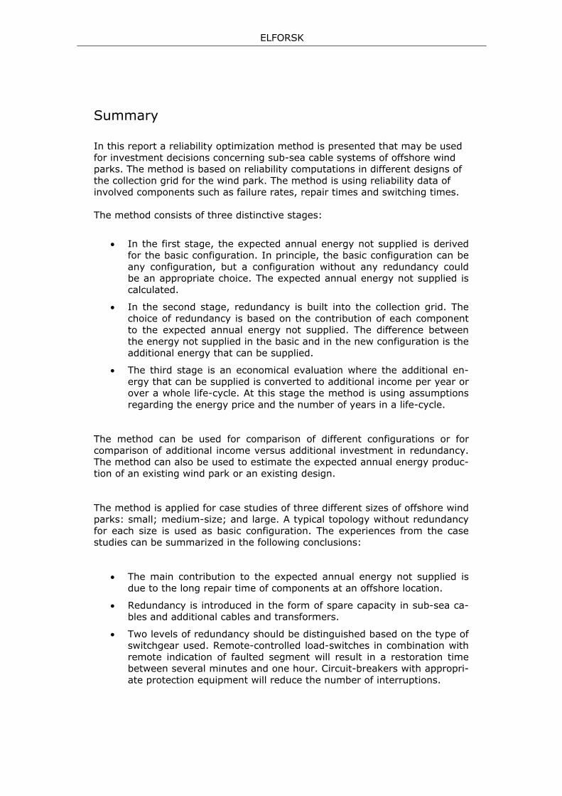
Summary

In this report a reliability optimization method is presented that may be used for investment decisions concerning sub-sea cable systems of offshore wind parks. The method is based on reliability computations in different designs of the collection grid for the wind park. The method is using reliability data of involved components such as failure rates, repair times and switching times. The method consists of three distinctive stages:

• In the first stage, the expected annual energy not supplied is derived for the basic configuration. In principle, the basic configuration can be any configuration, but a configuration without any redundancy could be an appropriate choice. The expected annual energy not supplied is calculated.

• In the second stage, redundancy is built into the collection grid. The choice of redundancy is based on the contribution of each component to the expected annual energy not supplied. The difference between the energy not supplied in the basic and in the new configuration is the additional energy that can be supplied.

• The third stage is an economical evaluation where the additional en-ergy that can be supplied is converted to additional income per year or over a whole life-cycle. At this stage the method is using assumptions regarding the energy price and the number of years in a life-cycle.

The method can be used for comparison of different configurations or for comparison of additional income versus additional investment in redundancy. The method can also be used to estimate the expected annual energy produc-tion of an existing wind park or an existing design.

The method is applied for case studies of three different sizes of offshore wind parks: small; medium-size; and large. A typical topology without redundancy for each size is used as basic configuration. The experiences from the case studies can be summarized in the following conclusions:

• The main contribution to the expected annual energy not supplied is due to the long repair time of components at an offshore location.

• Redundancy is introduced in the form of spare capacity in sub-sea ca-bles and additional cables and transformers.

• Two levels of redundancy should be distinguished based on the type of switchgear used. Remote-controlled load-switches in combination with remote indication of faulted segment will result in a restoration time between several minutes and one hour. Circuit-breakers with appropri-ate protection equipment will reduce the number of interruptions.

ELFORSK

• The additional gain of installing circuit-breakers is limited whereas the costs are typically very high. The costs may include the costs of switchgear able to withstand the higher fault currents.

• The gain of installing remote-controlled load-switches is significant as it reduces the duration of a production stoppage from several weeks or months to one hour or less.

• There is an optimal number of load-switches, above which additional ones only increase costs and complexity without significant further gains in expected annual energy production.

The method described in this report is a probabilistic method, which is inher-ently associated with uncertainty. Some care should be taken in comparing rather accurately known investment costs with uncertain gain in annual pro-duction. A small difference in total costs between two design alternatives should not be seen as significant and a base for an investment decision. There are, however, no general rules for how to handle this and a further discussion on this is beyond the scope of this report.

A change in input parameters (failure rate, expected repair time, investment costs, value of non-delivered energy) may impact the preferred design under the method described in this report. As several of the input parameters are in itself uncertain, this would introduce an additional uncertainty in the final de-cision. However, it is generally accepted in power system reliability that the outcome of the comparison is not impacted when the most-likely value is used for all input parameters and when the difference between the design is not too small.

ELFORSK

Sammanfattning

Rapporten presenterar en metod för tillförlitlighetsberäkningar som kan an-vändas vid beslut om investeringar i samband med sjökabelsystem för vind-kraftsparker till havs. Metoden är baserad på tillförlitlighetsberäkningar med olika utföranden av kabelkonfigurationer av vindkraftsparker. Metoden använ-der tillförlitlighetsdata på ingående komponenter såsom felfrekvens, repara-tionstid och omkopplingstid.

Metoden består av tre huvuddelar:

• I första delen beräknas den förväntade årliga icke levererade energin för en baskonfiguration. I princip kan baskonfigurationen vara vilken konfiguration som helst men en konfiguration utan redundans är ett lämpligt val. Den förväntade årliga icke levererade energin beräknas således.

• I del två bygger man in redundans i sjökabelsystemet. Valet av redun-dans är baserat på de bidrag som varje ingående komponent ger till den förväntade årliga icke levererade energin. Skillnaden mellan den icke levererade energin i baskonfigurationen och i den nya konfigura-tionen är den extra energin som kan bli levererad.

• Tredje delen är en ekonomisk utvärdering där den extra energin som kan bli levererad omräknas till en extra inkomst per år eller under hela dess livslängd. I detta steg görs antaganden om energipris och livs-längd.

Metoden kan användas för att jämföra olika konfigurationer eller för att jäm-föra extra inkomster mot extra investeringar i form av redundans. Metoden kan också användas till att ge en uppskattning av den förväntade årliga ener-giproduktionen för en existerande vindkraftspark eller en existerande konfigu-ration.

Exempel på metoden visas också i några fallstudier med tre olika storlekar på havsbaserade vindkraftsparker: liten; medel-stor; och stor. För varje park-storlek används en typisk konfiguration utan redundans som baskonfigura-tion. Erfarenheterna från dessa fallstudier kan summeras enligt följande:

• Det största bidraget till den förväntade årliga icke levererade energin är den långa reparationstiden för komponenter placerade ute till havs.

• Redundans introduceras i systemet genom extra kapacitet i sjökablar och extra kablar och transformatorer.

• Två nivåer av redundans kan urskiljas beroende på vilken typ av ställ-verk som används. Fjärrmanövrerade lastfrånskiljare i kombination med fjärrindikering av felande kabelsegment resulterar i återuppbygg-nadstider på några minuter upp till en timme. Brytare försedda med

ELFORSK

lämplig reläskyddsutrustning kommer däremot att reducera antalet avbrott.

• Den extra vinst som kan göras genom att installera brytare är begrän-sad då kostnaden är relativt hög. Kostnaden för detta kan även inklu-dera kostnaden för att ställverket ska tåla den högre felströmmen.

• Vinsten av att installera fjärrmanövrerade lastfrånskiljare är betydande då varaktigheten för ett produktionsstopp kan minskas från flera veck-or eller flera månader till en timme eller ännu mindre.

• Det finns ett optimalt antal av lastfrånskiljare som bör installeras. För många lastfrånskiljare ökar kostnaden och komplexiteten, men den förväntade årliga energiproduktionen ökar endast marginellt.

Metoden som beskrivs i denna rapport är en sannolikhetsmetod, där osäker-het är en faktor att beakta. Försiktighet måste därför gälla då man jämför kända investeringskostnader med osäkra resultat vad beträffar förbättring i årlig energiproduktion. En liten skillnad i den totala kostnaden mellan två kon-figurationer ska inte vara avgörande i ett investeringsbeslut. Med andra ord, så finns det inga generella regler för hur detta ska hanteras och ytterligare diskussion i ämnet är utanför arbetet i rapporten.

En förändring av en indataparameter (felfrekvens, förväntad reparationstid, investeringskostnad, värde av icke levererad energi) kan påverka den re-kommenderade konfigurationen. Då flertalet av indataparametrarna i sig är osäkra, kommer de att i sin tur generera ytterligare osäkerhet för det slutgil-tiga beslutet. Generellt sett i samband med tillförlitlighetsberäkningar i kraft-systemssammanhang, så påverkas inte resultatet av jämförelsen när värden med hög sannolikhet används som indataparametrar och när skillnaden mel-lan konfigurationer inte är alltför liten.

ELFORSK

Table of contents

1 Introduction 1 1.1 Background .................................................................................... 1 1.2 Study outline .................................................................................. 1 1.3 Assumptions and limitations.............................................................. 3

2 Description of the reliability method 6 2.1 Definition of the wind park configuration............................................. 6 2.2 Calculation of expected annual energy not supplied .............................. 6 2.3 Calculation of expected annual energy that can be supplied................... 9 2.4 Evaluation of additional income against additional investment.............. 10 2.5 Summary of uncertainties............................................................... 10

3 Basic configurations of offshore wind parks 11 3.1 Type 1: Small offshore wind parks ................................................... 11 3.2 Type 2: Medium-size offshore wind parks.......................................... 12 3.3 Type 3: Large offshore wind parks ................................................... 13

4 Data requirements 14

5 Reliability calculations of electrical interconnecting systems 16 5.1 Small offshore wind parks............................................................... 17 5.2 Medium-size offshore wind parks ..................................................... 20 5.3 Large offshore wind parks............................................................... 25 5.4 Summary of reliability calculations ................................................... 32

6 Additional income probability 34

7 Conclusions 37

8 References 39

ELFORSK

1 Introduction

The aim of this project is to present a method for reliability optimization of power supply of the electrical system of offshore wind parks, consisting of collection grids and AC sub-transmission grids.

1.1 Background Access to offshore wind turbines for service, maintenance, fault detections, reparations, etc. in the Nordic region, is strongly weather (and thus season) dependent. Therefore, it will be limited to a couple of months per year, basi-cally the summer months, [1] and [2]. This will cause longer repair times af-ter faults. This condition will also concern the internal collection cable system, the switchgear platform(s) and the sub-transmission cables to the PCC (Point of common coupling) station on shore. A large part of the collection grid con-sists of sub-sea cables, where it is possible that the failure rate of these ca-bles will be higher compared to cables on land. Movements in the sea floor can cause extra mechanical stress. Anchors from ships or devices from fishing boats can cause damages to the cables as it is experienced that offshore wind parks will attract fishes. However, today there is lack of knowledge regarding failure rates associated to sub-sea cables within wind parks.

Due to the large initial costs for the offshore wind park and also for the elec-trical equipment of the wind park, redundancy in these existing electrical sys-tems may not exist at all or redundancy exists, but maybe not on the most effective parts of the offshore wind park. The consequence is that the avail-ability of feeder sections, of wind park sections or of total wind parks are low.

1.2 Study outline The main issue of this study is to present a method for reliability calculations of different wind park configurations and sizes. The output results would be in additional income over the life-cycle time of the wind parks, as the energy not supplied, ENS (one of the measured quantities) is used in the study. A short description of the method is presented in chapter 2.

Three hypothetical wind park configurations are studied. These configurations are:

• Type 1: Small offshore wind park (40 MW) close to the grid on shore (less than 5 km)

• Type 2: Medium-size offshore wind park (160 MW) far away from the grid on shore (5 km to 25 km)

1

ELFORSK

• Type 3: Large offshore wind park (640 MW) far away from the grid on shore (5 km to 25 km)

The reason for this choice is that different wind park sites around the Swedish coast are being built or are discussed for exploitations, and these are all of different sizes and at different distances from the grid. As examples, Lillgrund with 110 MW is a medium-size offshore wind park and Kriegers Flak with about 600 MW is a large wind park, also at large distance from the grid.

The study has the following outline:

1. The basic topologies of the studied offshore wind parks, according to Type 1, Type 2 and Type 3 above, are determined, chapter 3.

2. Data is determined, both electrical parameters and reliability data, chapter 4. The reliability data consists of:

a. Failure rate, λ for the involved components in the transfer paths, see Appendix A.

b. Mean Time To Repair, MTTR for involved components. MTTR for the offshore equipment is estimated combined with new infor-mation from offshore wind parks, see Appendix B.

c. Mean Time To Switch, MTTS for involved circuit-breakers, dis-connectors and load-switches, see Appendix C.

3. Reliability calculations in Neplan software package, [13], are per-formed for all topologies, chapter 5. Important result for this study is the energy not supplied, ENS and the average service availability in-dex, ASAI for the alternative configurations of the wind parks. These values are used to measure the improvement in the availability be-tween different topologies. (Remark: the ENS is based on continuous rated power production and the value itself should not be used. This study is using this value for different topologies in order to compare and measure the improvement which each alternative configuration can offer.)

4. An alternative topology with redundant transfer paths compared to the previous topology is determined. This is made in terms of more sub-sea cables, circuit-breakers, disconnectors, load-switches, transform-ers, control systems, etc. In some of the alternatives, a redundancy transfer path is switched in after the protection system trips the faulty component. Other alternatives can require manual reconfiguration by load-switches in order to utilize the redundant transfer paths. Alternative topologies, which have too complicated redundant transfer paths or would cause a higher short-circuit capacity in the internal grid compared to the basic topologies, are not considered.

5. Stated as examples in chapter 6, one for each type of wind park con-figuration given above, it is calculated what these alternative topolo-

2

ELFORSK

gies can mean in additional annual supplied energy, and to be com-pared to additional equipment required for the redundancy of the elec-trical collection system.

1.3 Assumptions and limitations 1. The study is analysing the reliability of the electrical system contain-

ing the collection cable grid, switchgear and transformers on plat-forms (if any) and the sub-transmission cables to a land station. The study is therefore limited by the different delivery points such as the connection in the tower bottom of the wind turbines in one end and the switchgear in the PCC in the other end (the busbar in the grid station on shore is not included).

2. The wind turbines used in the study are rated 3.33 MW each and connected to a Medium Voltage, MV collection grid of 36 kV. It is as-sumed that each wind turbine has a load-switch at the delivery point, typically in the tower bottom. The distance between two wind turbines is 1 km.

3. It is assumed that there is additional High Voltage, HV equipment in each substation, other than circuit-breakers and disconnectors, such as earth-disconnectors, surge arresters, instrument transformers, etc. It is found by experiences that the number of failures in this equipment is small compared with the number of failures in cables. Therefore, this equipment is normally neglected in this type of stud-ies, alternatively those failures are considered to be included in the failure rate of the cables. The eventual contribution of station-based equipment is however less than the uncertainty in the failure rate of the undersea cables. It is also in this study assumed that this equipment have a low contribution to the energy not supplied and therefore neglected in this study.

4. The sub-transmission cable from a platform to shore is operated at a transmission voltage of 150 kV.

5. All included cables are assumed to be 3 core cables with sheath and armour.

6. Failure rates for electrical apparatuses (sub-sea cables excluded) are taken from corresponding equipment from land based distribution and industrial systems. (It might be argued that the environmental stress at offshore exploitation will in a longer time perspective in-crease the failure rates, but no quantitative information on this is available.)

7. A recent study by Strathclyde university, [15] has been used for 1 km sub-sea cable values for time between failure between 90 and 275 year (0.00365 to 0.01095 failure/year and km). According to the authors of that study, these values were based on practical ex-perience with sub-sea cables. For this study a value somewhere within this range has been used: 125 year (0.008 failure/year,km).

3

ELFORSK

8. Repair times can be found from experiences in distribution and in-dustrial system as well. However, for offshore wind parks, it will be assumed that these repair times will be more decisive of the access possibilities of the platform and the wind turbines, transportations at sea, waiting time for appropriate ship to be on duty and time for the actual repair. For the Nordic countries it is assumed that these ac-cess possibilities are reduced. In this study, therefore, longer repair times are used.

9. It is assumed that all the switchgear equipment on the platform or cables from the platform to shore can be repaired within 30 days (720 h) anytime of the year. However, for a platform transformer the repair time is assumed to be 6 months (4320 h) as faulty plat-form transformers may require replacements. Availability of spare transformers, lifting and shipping arrangements are quite uncertain. Therefore, a long repair time is assumed.

10. For equipment placed inside the wind turbine or cables from the wind turbines to shore/platform, the access possibilities are assumed to be worse. It is reported from one offshore wind park in Denmark that the access to the wind turbines from the sea were not possible during 40 % of that perticular year of study (note that the total availability of the wind turbines were not reported). Therefore, a waiting time is derived and added to the repair time. For six months of the year during the spring and summer seasons, it is assumed that the repair time is 30 days without any waiting time, except the last month of the summer season, where repair can not be finalized before the winter season and the waiting time for this month is 6 months. Further, during the autumn and winter (six months) the reparations may be postponed until spring. Therefore these months have waiting times, falling from 5.5 months (average of 6 months in the beginning and 5 months in the end of the month) to 0.5 month. The average waiting time for one year is calculated as:

( )days60months2

12

i5.66

yearpertimewaiting

6

1i ==

−+

=∑=

The average waiting time of 60 days is added to the repair time of 30 days and the final repair time is 90 days (2160 h) for these type of components.

11. It is assumed that a circuit-breaker is more expensive than a load-switch. As the problem for an offshore wind park is the long repara-tion time, a short interruption due to switching of load-switches (in-stead of fast reconfiguration by circuit-breakers) has minor effect on the reliability. Therefore, the collection grid is normally operating in a radial string and faults in the string are isolated by a circuit-breaker on a platform or on land. Remote controlled load-switches with over-current indicators can inform where faults are located. Af-ter reconfiguration, the remaining part of the feeder string goes into

4

ELFORSK

operation again. This switching duration time for a load-switch, from fault to operation again, is assumed to be 20 minutes.

12. The analysis presents the expected annual energy not supplied, ENS and the average service availability index, ASAI, and it is the first quantity what is used to compare different alternatives to each other and to identify components which have a high contribution to the expected annual energy not supplied.

13. The life cycle for an offshore wind park is assumed to be 20 years.

14. In the examples, where the expected additional income due to higher availabilities is calculated, the energy price for an Independ-ent Producer, IP is assumed to be 0.03 € per kWh (about 0.3 SEK per kWh).

5

ELFORSK

2 Description of the reliability method

The reliability method used in this study consists of the following parts:

1. Definition of the wind park configuration

2. Calculation of expected annual energy not supplied

3. Calculation of expected annual energy that can be supplied

4. Evaluation of additional income against additional investment

2.1 Definition of the wind park configuration The studied configurations of the offshore wind parks are set up in Neplan, including sub-sea cables, switchgear, power transformers and wind turbines. Basic topologies for small, medium-size and large wind parks, respectively are set up. Wind turbines are assumed to be operating at rated power level.

2.2 Calculation of expected annual energy not supplied Reliability data is added to these components in the Neplan set up, which should be included in the reliability evaluation. The reliability data is:

• Failure rate, λ in failure/yr (or failure/yr,km for cables)

• Mean time to repair, MTTR in h

• Mean time to switch, MTTS in min (for circuit-breakers and load-switches)

For a radial distribution system, which is comparable to a collection grid of an offshore wind park, with ‘i’ number of series components supplying load ‘s’ (or generator ‘s’ is the same), the ENS and the ASAI can be calculated as, [16]:

6

ELFORSK

%in100*8750

U8750ASAIload,forindextyavailabiliserviceAverage

MWh/yearinENSENSload,forsuppliednotenergyAnnual

MWh/yearinU*LENScomponent,forsuppliednotenergyAnnual

MWinLload,Average

hinλ

r*λ

λU

rload,fortimeoutageAverage

h/yearinr*λUload,fortimeoutageannualAverage

h/yearinr*λUcomponent,fortimeoutageannualAverage

arfailure/yeinλλload,forratefailureAverage

ss

iis

iii

i

ii

iii

s

ss

iiis

iii

iis

−=

=

=

==

=

=

=

∑

∑∑∑

∑

Example:

Consider a radial system of series components interconnecting a generator to a grid, as shown in figure 1. The average generation is assumed to be 5 MW.

Grid Cable, 10 km Generator, 5 MW Circuit-breaker 2Circuit-breaker 1

Statistic data λ=0.04 failure/year

MTTR=10 h L=5 MW

λ=0.04 failure/year MTTR=20 h L=5 MW

0.008 failure/year,km=>λ=0.08 failure/year MTTR=20 h L=5 MW

Derived data

U=0.4 h/year ENS=2 MWh/year



λs=0.16 failure/year Us=2.8 h/year rs=17.5 h/year ENSs=14 MWh/year ASAIs=99.97 %

Figure 1: Example – a system of 3 series components

Circuit-breaker 1:

The circuit-breaker is assumed to have 25 years to a failure, e.g. the failure rate, λ is 0.04 failure/year and the MTTR is 10 h.

The following can be derived:

7

ELFORSK

year/MWh0.2U*LENS

MW5L,loadAverage

year/h4.0U,timeoutageannualAverage

h10MTTR,repairtotimeMean

year/failure04.0λ,rateFailure

111

1

1

1

1

==

=

=

=

=

Cable:

The cable is 10 km and have a statistic information of 125 year and km to a failure. The MTTR is 20 h. This means:

year/MWh0.8U*LENS

MW5L,loadAverage



year/failure08.0*km10*km,year/failure008.0λ,rateFailure

222

2

2

2

2

==

=

=

=

==

Circuit-breaker 2:

The circuit-breaker have a statistic failure information of 25 year to a failure and the MTTR is 20 h. This means for this component:

year/MWh0.4U*LENS

MW5L,loadAverage



year/failure04.0λ,rateFailure

333

3

3

3

3

==

=

=

=

=

Total for the generator:

Together, the three series components create a system where the reliability results for the generator can be derived as:

8

ELFORSK

%97.99100*8750

U8750ASAI,indextyavailabiliserviceAverage

year/MWh0.14ENSENS,suppliednotEnergy

h5.1728.02.5

λU

r,timeoutageAverage

year/h8.2r*λU,timeoutageannualAverage

year/failure16.0λλ,ratefailureAverage

s

3

1iis

s

ss

i

3

1iis

3

1iis

=−

=

==

===

==

==

∑

∑

∑

=

=

=

As can be seen from the example above, the highest contribution to the total ENS is the cable. Addition of components especially series components, ex-pected to have outages, will increase the energy not supplied. Addition of parallel components creating a parallel transfer path which can be used sepa-rately during failures of the other circuit, are reducing the energy not sup-plied. At full redundant transfer path, where the parallel circuit is completely taking over the transfer path, the contribution to the energy not supplied is zero or at a small value caused by the switching times of those couplers in-volved in the reconfiguration of the path. This is not shown in this report.

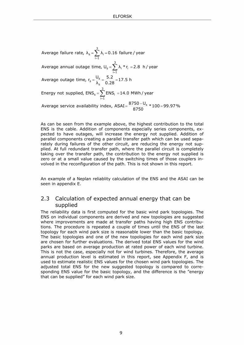
An example of a Neplan reliablity calculation of the ENS and the ASAI can be seen in appendix E.

2.3 Calculation of expected annual energy that can be supplied

The reliability data is first computed for the basic wind park topologies. The ENS on individual components are derived and new topologies are suggested where improvements are made at transfer paths having high ENS contribu-tions. The procedure is repeated a couple of times until the ENS of the last topology for each wind park size is reasonable lower than the basic topology. The basic topologies and one of the new topologies for each wind park size are chosen for further evaluations. The derived total ENS values for the wind parks are based on average production at rated power of each wind turbine. This is not the case, especially not for wind turbines. Therefore, the average annual production level is estimated in this report, see Appendix F, and is used to estimate realistic ENS values for the chosen wind park topologies. The adjusted total ENS for the new suggested topology is compared to corre-sponding ENS value for the basic topology, and the difference is the ”energy that can be supplied” for each wind park size.

9

ELFORSK

2.4 Evaluation of additional income against additional in-vestment

The “energy that can be supplied” values are converted to additional income for a small, medium-size and large wind park. This is based on estimated en-ergy price and expected life-cycle of the wind turbines. The additional income is then compared to the additional equipment required for each wind park size to fulfil the new wind park configurations.

2.5 Summary of uncertainties The reliability method used here is going through a couple of steps as de-scribed above. In the method, there is assumptions made which create uncer-tainties, and these can be summarized as follows:

• Uncertainty in used failure rates.

• Uncertainty in used MTTR.

• Uncertainty in derived ENS after assumed average production level of the wind turbines.

• Uncertainty in used energy price.

• Uncertainty in used life-cycle time.

• Uncertainty in derived additional income during a life-cycle.

• Uncertainty in estimated additional cost in redundancies.

However, with these uncertainties in mind, the method is a strong feature to find components with high contribution to the total ENS and to compare dif-ferent topologies. It can also give a first indication if additional investment in redundancy is profitable or not.

10

ELFORSK

3 Basic configurations of offshore wind parks

Three types of wind park are studied. These are:

1. Type 1: Small offshore wind park (40 MW) close to the onshore grid (less than 5 km)

2. Type 2: Medium large offshore wind park (160 MW) far from the on-shore grid (5 km to 25 km)

3. Type 3: Large offshore wind park (640 MW) far from the onshore grid (5 km to 25 km)

3.1 Type 1: Small offshore wind parks Type 1 can be characterized as being small (in number of wind turbines and in installed MW) and has short distance (4 km) to PCC. The wind turbines are connected to PCC with one feeder cable.

Wind turbine

4 km

PCC

Switchgear

Bus

Cable 40 MW in 12 wind turbines

Wind turbine area

PCC

Figure 2: Basic configuration of a small wind park (type 1)

11

ELFORSK

3.2 Type 2: Medium-size offshore wind parks Type 2 can be characterized as being medium-size and has long distance (20 km) to PCC. The wind turbines are connected in a feeder fork to a platform and one sub-transmission cable to PCC. The average feeder cable length is assumed to be 2 km.

Offshore platform

Transformer

2 km

PCC

160 MW in 4 feeders 40 MW in each feeder of 12 wind turbines

20 km

Platform Wind turbine area

PCC

Figure 3: Basic configuration of a medium-size wind park (type 2)

12

ELFORSK

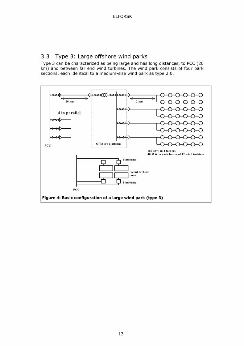
3.3 Type 3: Large offshore wind parks Type 3 can be characterized as being large and has long distances, to PCC (20 km) and between far end wind turbines. The wind park consists of four park sections, each identical to a medium-size wind park as type 2.0.

Offshore platform

2 km

PCC

160 MW in 4 feeders 40 MW in each feeder of 12 wind turbines

20 km

4 in parallel

Platforms

Platforms

Wind turbine area

PCC Figure 4: Basic configuration of a large wind park (type 3)

13

ELFORSK

4 Data requirements

Data, which is required, is electrical data for cables and transformers, failure rates (λ) and repair times (MTTR) for cables, transformers, circuit-breakers, load-switches and busbars in offshore environment and switching times (MTTS) for circuit-breakers and load-switches.

Electrical parameters:

Transformer:

For the platform transformers the following data is used:

• Rated power is 160 MVA

• uk is 12 %

Cables:

For the sub-sea cables, which are defined from cable area and voltage level, the following data is used:

Copper core cables with a current density of 1.25 A/mm2 are used in the core area determination.

36 kV wind turbine interconnecting cables and feeder cables:

• Cable for 20 MW Nominal current 320 A => 250 mm2; 300 mm2 is used



150 kV sub-transmission cables:


From the Cu core area, the series resistance per km is derived. For the series reactance per km and the shunt capacitance per km, these are set to 0.110 ohm per km and 0.200 µF per km, respectively, for all used cables.

14

ELFORSK

For the current limits of the cables, the final area, the current density, the rating factor of 1.05 due to sea water temperature and the rating factor 0.9 due to the screen and the armour, have been used.

The chosen electrical data in this study is shown in appendix D.

Statistical or assumed interruption data:

The failure rate, the repair time and the switching time data used in the study is shown in appendices A, B and C.

• In the land station, repair times for distribution and industrial systems

are used.

• For sub-sea cables from shore to a platform and equipment on the platform (excluding platform transformers), the repair times of 720 hours (30 days) are used.

• For platform transformers, the repair times of 4320 hours (180 days) are used. This repair time include delay time for replacement which re-quires lifting and shipping arrangements and availability of spare units.

• For sub-sea cables from the platform to the wind turbines, intercon-necting wind turbine cables and equipment placed in the tower bottom of the wind turbines, the repair times of 2160 hours (90 days) are used. This repair time includes a waiting time of 1440 hours (60 days) due to delays cause during the winter seasons.

15

ELFORSK

5 Reliability calculations of electrical interconnecting systems

The power flow and the reliability calculation modules of Neplan are used in the aim of deriving the improved hourly operations per year for each basic and redundant alternative configuration.

The reliability calculation is performed with the following general settings:

System state analysis: Capacity flow (current limit check)

Failure model: Single independent failure

Loading limit: Long-term 100 %

Duration to remote switching: 20 minutes

This set up means that the probability of interruptions of the network is ex-amined for single outages and power supply is not allowed at over-loaded conditions of redundant components. The duration to remote switching is used for those load-switches used in the cable system, which means that re-configuration by load-switches can not be made immediately. The duration of remote switching is the same as Mean Time To Switching, MTTS.

Results from Neplan Reliability are given for the total system and for each component in the studied network. The results can be used to identify com-ponents which have high contribution to the derived unavailability.

In the following analysis, the small wind park including some alternatives is examined first. This type 1 alternative, which results in less expected annual energy not supplied, is reused in the medium-size wind parks. Further, the type 2 alternative of less expected annual energy not supplied, is reused in the large wind park part.

The analysis is made at full MW production and the average values of the in-terruption data according to appendices A, B and C are used. The presented expected annual energy not supplied should only be used in order to compare different alternatives and also to identify components which have high contri-bution to the expected annual energy not supplied.

16

ELFORSK

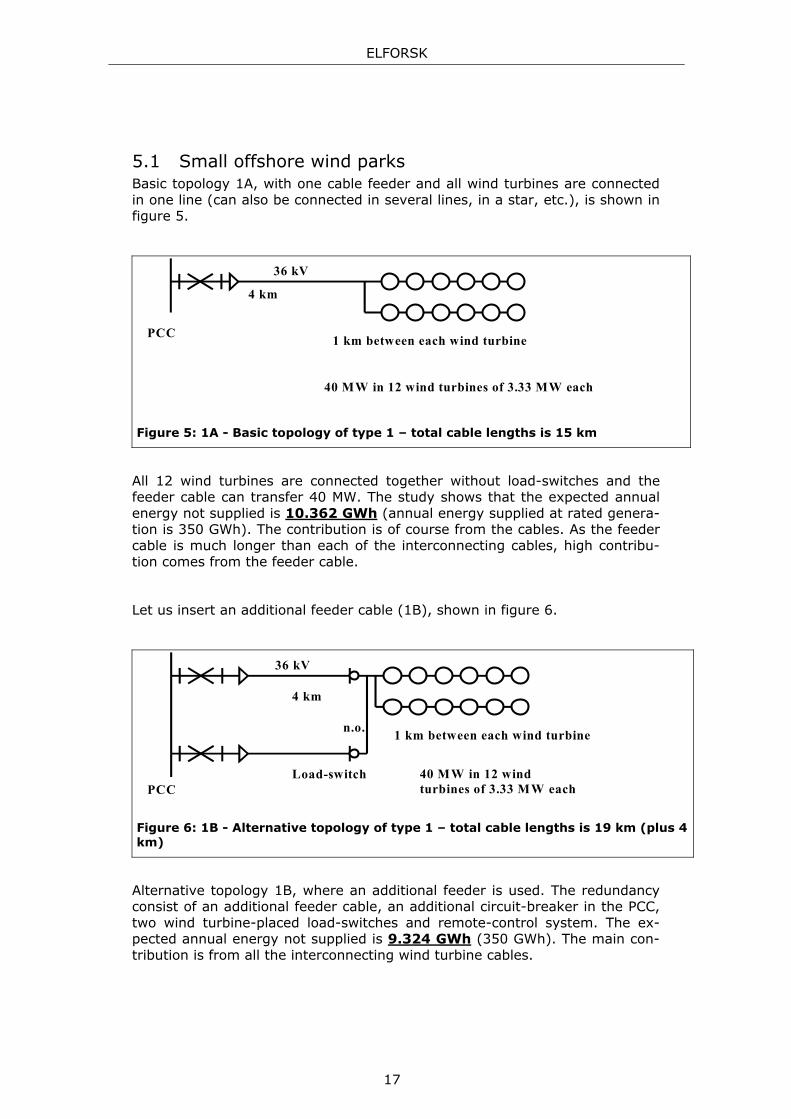
5.1 Small offshore wind parks Basic topology 1A, with one cable feeder and all wind turbines are connected in one line (can also be connected in several lines, in a star, etc.), is shown in figure 5.

36 kV

1 km between each wind turbine

4 km

PCC

40 MW in 12 wind turbines of 3.33 MW each

Figure 5: 1A - Basic topology of type 1 – total cable lengths is 15 km

All 12 wind turbines are connected together without load-switches and the feeder cable can transfer 40 MW. The study shows that the expected annual energy not supplied is 10.362 GWh (annual energy supplied at rated genera-tion is 350 GWh). The contribution is of course from the cables. As the feeder cable is much longer than each of the interconnecting cables, high contribu-tion comes from the feeder cable.

Let us insert an additional feeder cable (1B), shown in figure 6.

Load-switch

n.o.

36 kV

1 km between each wind turbine

4 km

PCC 40 MW in 12 wind turbines of 3.33 MW each

Figure 6: 1B - Alternative topology of type 1 – total cable lengths is 19 km (plus 4 km)

Alternative topology 1B, where an additional feeder is used. The redundancy consist of an additional feeder cable, an additional circuit-breaker in the PCC, two wind turbine-placed load-switches and remote-control system. The ex-pected annual energy not supplied is 9.324 GWh (350 GWh). The main con-tribution is from all the interconnecting wind turbine cables.

17

ELFORSK

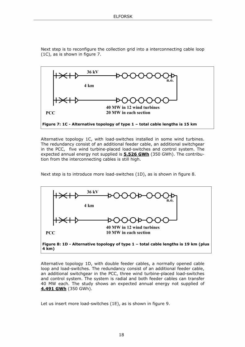
Next step is to reconfigure the collection grid into a interconnecting cable loop (1C), as is shown in figure 7.

n.o.

36 kV

4 km

PCC 40 MW in 12 wind turbines 20 MW in each section

Figure 7: 1C - Alternative topology of type 1 – total cable lengths is 15 km

Alternative topology 1C, with load-switches installed in some wind turbines. The redundancy consist of an additional feeder cable, an additional switchgear in the PCC, five wind turbine-placed load-switches and control system. The expected annual energy not supplied is 5.526 GWh (350 GWh). The contribu-tion from the interconnecting cables is still high.

Next step is to introduce more load-switches (1D), as is shown in figure 8.

n.o.

36 kV

4 km

PCC 40 MW in 12 wind turbines 10 MW in each section

Figure 8: 1D - Alternative topology of type 1 – total cable lengths is 19 km (plus 4 km)

Alternative topology 1D, with double feeder cables, a normally opened cable loop and load-switches. The redundancy consist of an additional feeder cable, an additional switchgear in the PCC, three wind turbine-placed load-switches and control system. The system is radial and both feeder cables can transfer 40 MW each. The study shows an expected annual energy not supplied of 4.491 GWh (350 GWh).

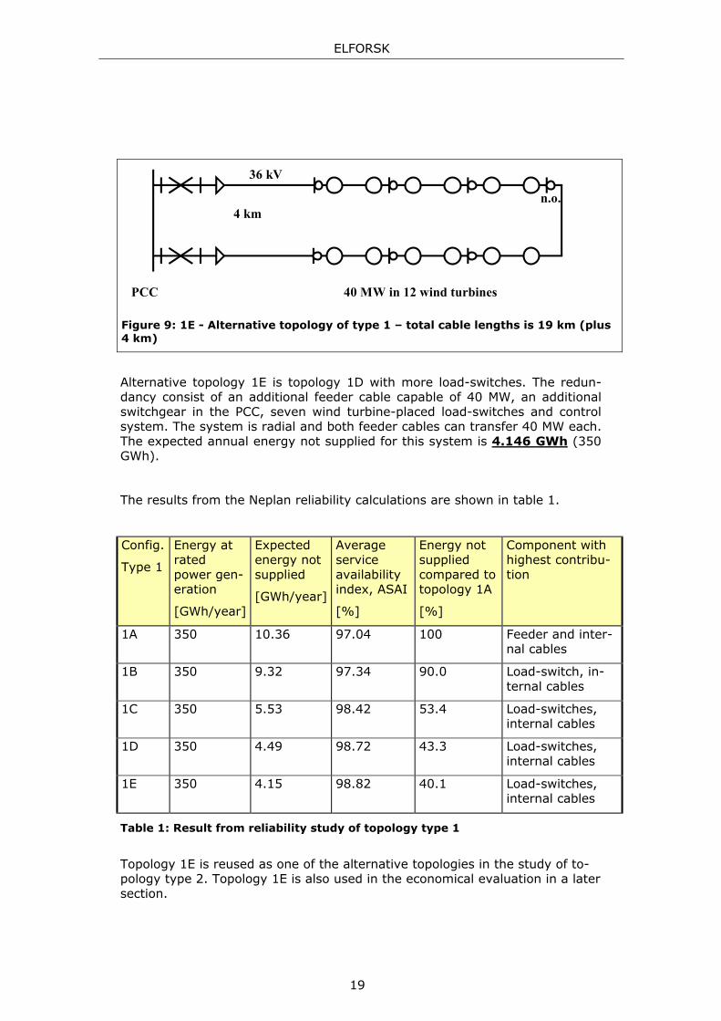
Let us insert more load-switches (1E), as is shown in figure 9.

18

ELFORSK

n.o.

36 kV

4 km

PCC 40 MW in 12 wind turbines

Figure 9: 1E - Alternative topology of type 1 – total cable lengths is 19 km (plus 4 km)

Alternative topology 1E is topology 1D with more load-switches. The redun-dancy consist of an additional feeder cable capable of 40 MW, an additional switchgear in the PCC, seven wind turbine-placed load-switches and control system. The system is radial and both feeder cables can transfer 40 MW each. The expected annual energy not supplied for this system is 4.146 GWh (350 GWh).

The results from the Neplan reliability calculations are shown in table 1.

Config.

Type 1

Energy at rated power gen-eration

[GWh/year]

Expected energy not supplied

[GWh/year]

Average service availability index, ASAI

[%]

Energy not supplied compared to topology 1A

[%]

Component with highest contribu-tion

1A 350 10.36 97.04 100 Feeder and inter-nal cables

1B 350 9.32 97.34 90.0 Load-switch, in-ternal cables

1C 350 5.53 98.42 53.4 Load-switches, internal cables

1D 350 4.49 98.72 43.3 Load-switches, internal cables

1E 350 4.15 98.82 40.1 Load-switches, internal cables

Table 1: Result from reliability study of topology type 1

Topology 1E is reused as one of the alternative topologies in the study of to-pology type 2. Topology 1E is also used in the economical evaluation in a later section.

19

ELFORSK

Remarks:

If the wind park is connected to a strong grid, the short-circuit capacity can be high within the wind park. Adding parallel paths may increase the short-circuit current above the rating of the switchgear. To prevent this, the redun-dant components are operated normally-open on one side. This will prevent them to contribute to the fault current, whereas faults in these redundant components will still be detected.

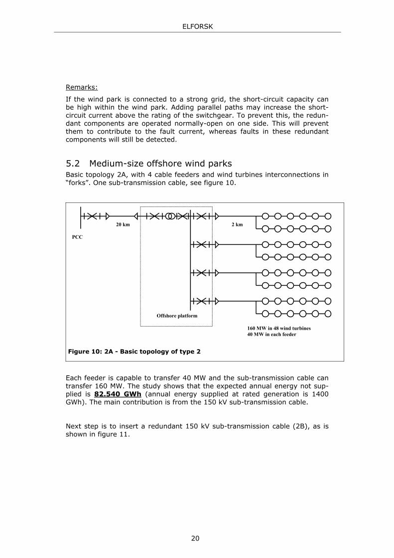
5.2 Medium-size offshore wind parks Basic topology 2A, with 4 cable feeders and wind turbines interconnections in “forks”. One sub-transmission cable, see figure 10.

PCC

160 MW in 48 wind turbines 40 MW in each feeder

Offshore platform

20 km 2 km

Figure 10: 2A - Basic topology of type 2

Each feeder is capable to transfer 40 MW and the sub-transmission cable can transfer 160 MW. The study shows that the expected annual energy not sup-plied is 82.540 GWh (annual energy supplied at rated generation is 1400 GWh). The main contribution is from the 150 kV sub-transmission cable.

Next step is to insert a redundant 150 kV sub-transmission cable (2B), as is shown in figure 11.

20

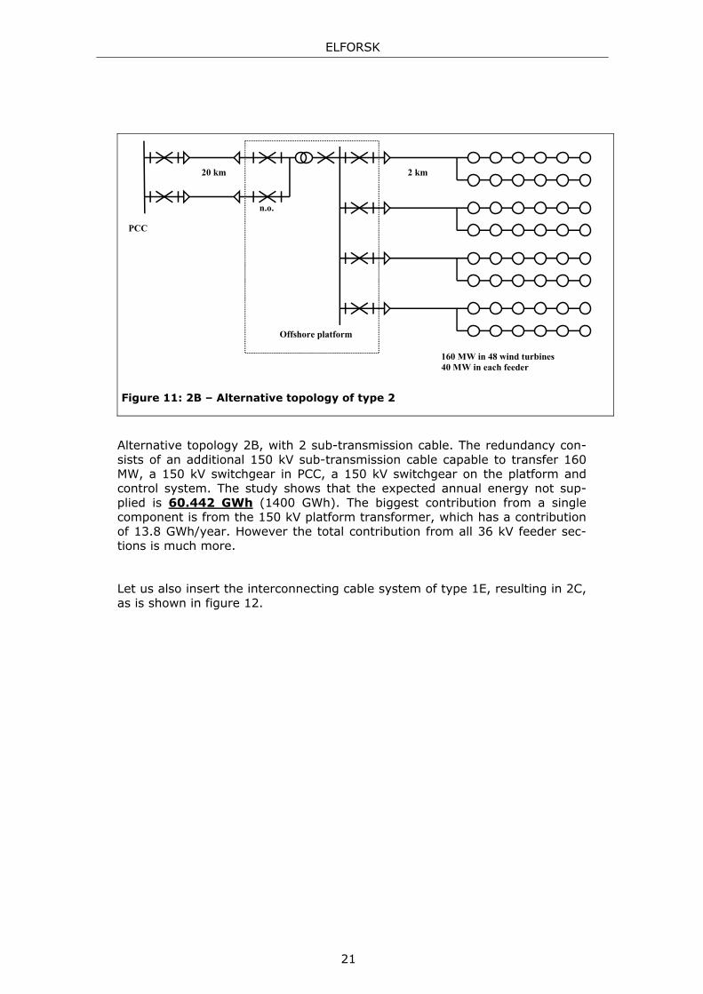
ELFORSK

Offshore platform

n.o.

PCC


20 km 2 km

Figure 11: 2B – Alternative topology of type 2

Alternative topology 2B, with 2 sub-transmission cable. The redundancy con-sists of an additional 150 kV sub-transmission cable capable to transfer 160 MW, a 150 kV switchgear in PCC, a 150 kV switchgear on the platform and control system. The study shows that the expected annual energy not sup-plied is 60.442 GWh (1400 GWh). The biggest contribution from a single component is from the 150 kV platform transformer, which has a contribution of 13.8 GWh/year. However the total contribution from all 36 kV feeder sec-tions is much more.

Let us also insert the interconnecting cable system of type 1E, resulting in 2C, as is shown in figure 12.

21

ELFORSK

Offshore platform

n.o.

PCC


20 km n.o.2 km

n.o.2 km

n.o.2 km

n.o.2 km

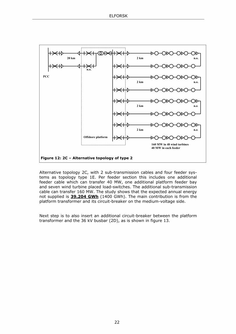
Figure 12: 2C – Alternative topology of type 2

Alternative topology 2C, with 2 sub-transmission cables and four feeder sys-tems as topology type 1E. Per feeder section this includes one additional feeder cable which can transfer 40 MW, one additional platform feeder bay and seven wind turbine placed load-switches. The additional sub-transmission cable can transfer 160 MW. The study shows that the expected annual energy not supplied is 39.204 GWh (1400 GWh). The main contribution is from the platform transformer and its circuit-breaker on the medium-voltage side.

Next step is to also insert an additional circuit-breaker between the platform transformer and the 36 kV busbar (2D), as is shown in figure 13.

22

ELFORSK

n.o.

Offshore platform

n.o.

PCC


20 km n.o.2 km

n.o.2 km

n.o.2 km

n.o.2 km

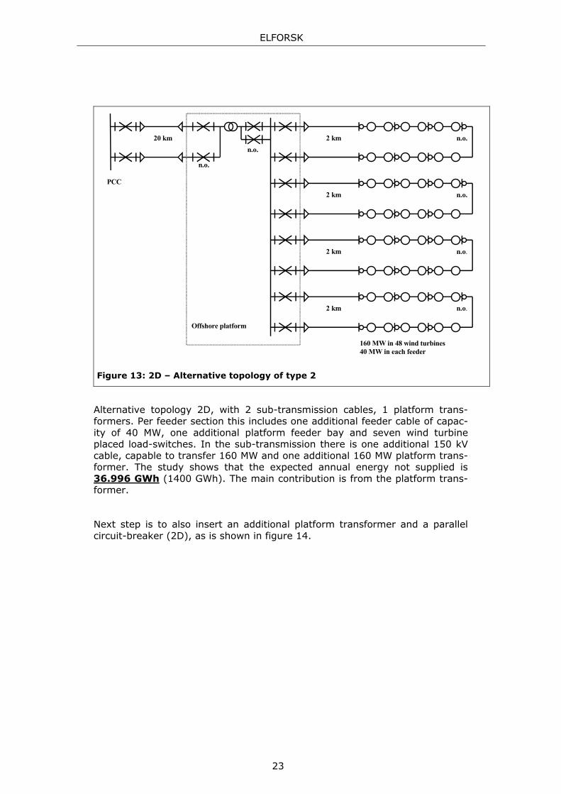
Figure 13: 2D – Alternative topology of type 2

Alternative topology 2D, with 2 sub-transmission cables, 1 platform trans-formers. Per feeder section this includes one additional feeder cable of capac-ity of 40 MW, one additional platform feeder bay and seven wind turbine placed load-switches. In the sub-transmission there is one additional 150 kV cable, capable to transfer 160 MW and one additional 160 MW platform trans-former. The study shows that the expected annual energy not supplied is 36.996 GWh (1400 GWh). The main contribution is from the platform trans-former.

Next step is to also insert an additional platform transformer and a parallel circuit-breaker (2D), as is shown in figure 14.

23

ELFORSK

Offshore platform

n.o. n.o.

PCC


20 km n.o.2 km

n.o.2 km

n.o.2 km

n.o.2 km

Figure 14: 2E – Alternative topology of type 2

Alternative topology 2E, with 2 sub-transmission cables, 2 platform trans-formers. Per feeder section this includes one additional feeder cable of capac-ity of 40 MW, one additional platform feeder bay and seven wind turbine placed load-switches. In the sub-transmission there is one additional 150 kV cable, capable to transfer 160 MW and one additional 160 MW platform trans-former. The study shows that the expected annual energy not supplied is 19.873 GWh (1400 GWh). The main contribution is from the load-switches.

The results from the Neplan reliability calculations are shown in table 2.

Config.

Type 2

Energy at rated power gen-eration

[GWh/year]


[GWh/year]

ASAI

[%]

Energy not supplied compared to 2A

[%]

Component with high-est contribution

2A 1400 82.54 94.10 100 Sub-transmission cable

2B 1400 60.44 95.68 73.2 4 feeder cables

2C 1400 39.20 97.20 47.5 Platform transformer, 36 kV switchgear

2D 1400 37.00 97.36 44.8 Platform transformer

2E 1400 19.87 98.58 24.1 Load-switches

Table 2: Result from reliability study of topology type 2

24

ELFORSK

Topology 2E is used in the economical evaluation in a later section.

Remarks:

Regarding the short-circuit capacity of type 2, non of the alternatives 2B – 2E will change the level as all reconfigurations with circuit-breakers or load-switches are operated in radially.

5.3 Large offshore wind parks Basic topology with 4 subsystems, each with a platform switchgear and wind turbines in a fork as figure 15.

Offshore platform

PCC 160 MW in 48 wind turbines 40 MW in each feeder

4 in parallel

640 MW in 4 subsystem 160 MW in each subsystem

20 km 2 km

Figure 15: 3A - Basic topology of type 3

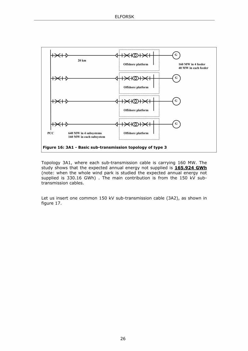
This is four times the same topology as 2A. The expected annual energy not supplied (at rated operation) will be 4 times 82.54 GWh, which is 330.16 GWh (annual energy supplied at rated generation is 5600 GWh).

The basic topology studied, will be divided into a first part where the sub-transmission is studied and a second part where a large wind park is studied. The basic sub-transmission configuration will be as figure 16.

25

ELFORSK

PCC

160 MW in 4 feeder 40 MW in each feeder

640 MW in 4 subsystems 160 MW in each subsystem

G

Offshore platform

G

Offshore platform

G

Offshore platform

G

Offshore platform

20 km

Figure 16: 3A1 - Basic sub-transmission topology of type 3

Topology 3A1, where each sub-transmission cable is carrying 160 MW. The study shows that the expected annual energy not supplied is 165.924 GWh (note: when the whole wind park is studied the expected annual energy not supplied is 330.16 GWh) . The main contribution is from the 150 kV sub-transmission cables.

Let us insert one common 150 kV sub-transmission cable (3A2), as shown in figure 17.

26

ELFORSK

Offshore platform

Offshore platform

Offshore platform

Offshore platform

8 km

8 km

8 km

20 km

n.o.

n.o.

n.o.

n.o.

PCC



G

G

G

G

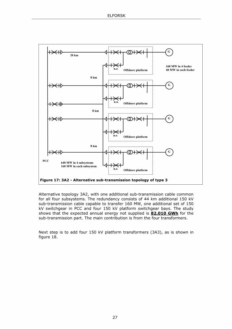
Figure 17: 3A2 - Alternative sub-transmission topology of type 3

Alternative topology 3A2, with one additional sub-transmission cable common for all four subsystems. The redundancy consists of 44 km additional 150 kV sub-transmission cable capable to transfer 160 MW, one additional set of 150 kV switchgear in PCC and four 150 kV platform switchgear bays. The study shows that the expected annual energy not supplied is 82.010 GWh for the sub-transmission part. The main contribution is from the four transformers.

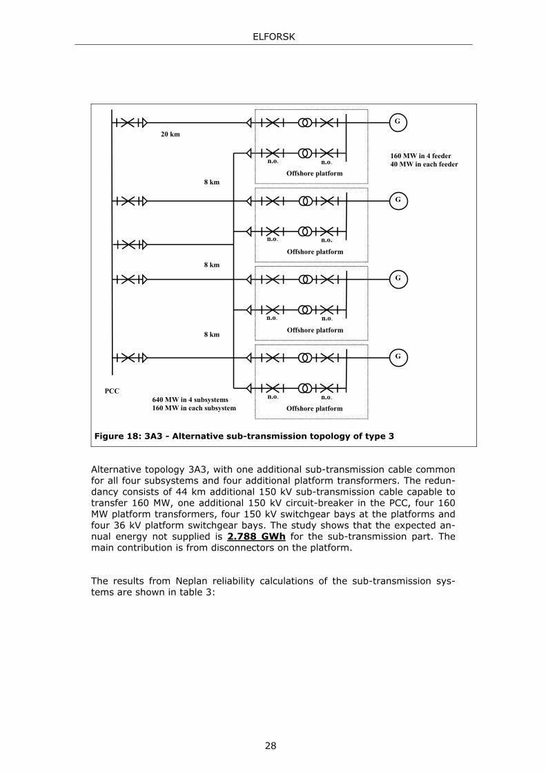
Next step is to add four 150 kV platform transformers (3A3), as is shown in figure 18.

27

ELFORSK

n.o.

n.o.

n.o.

Offshore platform

Offshore platform

Offshore platform

n.o.Offshore platform

n.o.

n.o.

n.o.

n.o.

PCC



G

G

G

G

20 km

8 km

8 km

8 km

Figure 18: 3A3 - Alternative sub-transmission topology of type 3

Alternative topology 3A3, with one additional sub-transmission cable common for all four subsystems and four additional platform transformers. The redun-dancy consists of 44 km additional 150 kV sub-transmission cable capable to transfer 160 MW, one additional 150 kV circuit-breaker in the PCC, four 160 MW platform transformers, four 150 kV switchgear bays at the platforms and four 36 kV platform switchgear bays. The study shows that the expected an-nual energy not supplied is 2.788 GWh for the sub-transmission part. The main contribution is from disconnectors on the platform.

The results from Neplan reliability calculations of the sub-transmission sys-tems are shown in table 3:

28

ELFORSK

Configuration

Type 3

Expected annual energy not sup-plied

[GWh/year]

Component with high-est contribution

Expected energy not supplied compared to topology 3A

[%]

3A1 165.92 Sub-transmission ca-bles

100

3A2 82.01 Platform transformers 49.4

3A3 2.79 Disconnectors 1.7

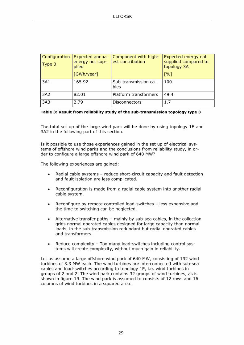
Table 3: Result from reliability study of the sub-transmission topology type 3

The total set up of the large wind park will be done by using topology 1E and 3A2 in the following part of this section.

Is it possible to use those experiences gained in the set up of electrical sys-tems of offshore wind parks and the conclusions from reliability study, in or-der to configure a large offshore wind park of 640 MW? The following experiences are gained:

• Radial cable systems – reduce short-circuit capacity and fault detection and fault isolation are less complicated.

• Reconfiguration is made from a radial cable system into another radial cable system.

• Reconfigure by remote controlled load-switches – less expensive and the time to switching can be neglected.

• Alternative transfer paths – mainly by sub-sea cables, in the collection grids normal operated cables designed for large capacity than normal loads, in the sub-transmission redundant but radial operated cables and transformers.

• Reduce complexity – Too many load-switches including control sys-tems will create complexity, without much gain in reliability.

Let us assume a large offshore wind park of 640 MW, consisting of 192 wind turbines of 3.3 MW each. The wind turbines are interconnected with sub-sea cables and load-switches according to topology 1E, i.e. wind turbines in groups of 2 and 2. The wind park contains 32 groups of wind turbines, as is shown in figure 19. The wind park is assumed to consists of 12 rows and 16 columns of wind turbines in a squared area.

29

ELFORSK

A group of 6 wind turbines, interconnected with totally 5 km sub-sea cables and 2 load-switches

Figure 19: 640 MW offshore wind park – 12 rows of 16 wind turbines in each row

Insert 40 MW feeder cables to each wind turbine group from platform switch-gears to load-switches at the first wind turbine in the group, as is shown in figure 20.

Figure 20: Large wind park – fed from platform busbars

Interconnect groups of wind turbines by sub-sea cables and normally opened load-switches inside the wind park, as is shown in figure 21. The number of load-switches and the interconnection can be discussed, but in this case to-pology 1E is used and the number of load-switches is 28.

30

ELFORSK

Figure 21: Large wind park – interconnected as topology 1E

Insert sub-transmission cable systems including one common alternative sub-transmission cable, according to topology 3B, as is shown in figure 22.

8 km

8 km

8 km

PCC

n.o.

n.o.

n.o.

n.o.

20 km

2 km

Figure 22: 3B – Topology for a large wind park, sub-transmission as 3A2

The expected annual energy not supplied for this large wind park is 157.113 GWh, which can be compared to the basic topology 3A, which is 330.64 GWh. The result of a large wind park can be seen in table 4.

31

ELFORSK

Config.

Type 3

Energy at rated power generation

[GWh/year]


[GWh/year]

ASAI

[%]

Energy not sup-plied compared to top. 3

[%]

Component with highest contribu-tion

3A 5600 330.16

(4 times top. 2A)

94.10 100 Sub-transmission cables

3B 5600 157.11 97.20 47.6 4 platform trans-formers

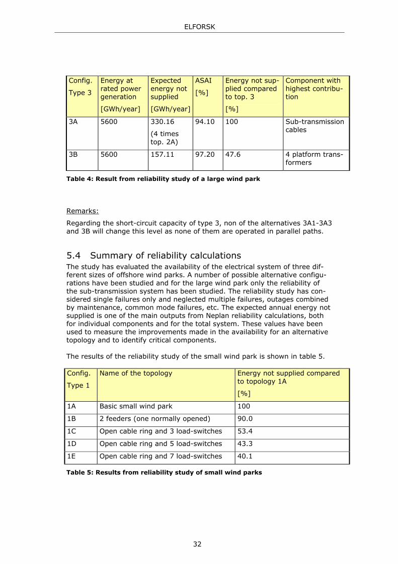
Table 4: Result from reliability study of a large wind park

Remarks:

Regarding the short-circuit capacity of type 3, non of the alternatives 3A1-3A3 and 3B will change this level as none of them are operated in parallel paths.

5.4 Summary of reliability calculations The study has evaluated the availability of the electrical system of three dif-ferent sizes of offshore wind parks. A number of possible alternative configu-rations have been studied and for the large wind park only the reliability of the sub-transmission system has been studied. The reliability study has con-sidered single failures only and neglected multiple failures, outages combined by maintenance, common mode failures, etc. The expected annual energy not supplied is one of the main outputs from Neplan reliability calculations, both for individual components and for the total system. These values have been used to measure the improvements made in the availability for an alternative topology and to identify critical components. The results of the reliability study of the small wind park is shown in table 5. Config.

Type 1

Name of the topology Energy not supplied compared to topology 1A

[%]

1A Basic small wind park 100

1B 2 feeders (one normally opened) 90.0

1C Open cable ring and 3 load-switches 53.4

1D Open cable ring and 5 load-switches 43.3

1E Open cable ring and 7 load-switches 40.1

Table 5: Results from reliability study of small wind parks

32

ELFORSK

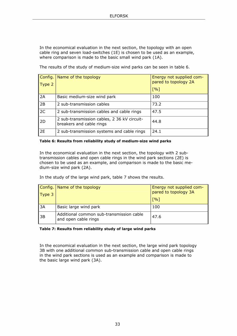
In the economical evaluation in the next section, the topology with an open cable ring and seven load-switches (1E) is chosen to be used as an example, where comparison is made to the basic small wind park (1A). The results of the study of medium-size wind parks can be seen in table 6. Config.

Type 2

Name of the topology Energy not supplied com-pared to topology 2A

[%]

2A Basic medium-size wind park 100

2B 2 sub-transmission cables 73.2

2C 2 sub-transmission cables and cable rings 47.5

2D 2 sub-transmission cables, 2 36 kV circuit-breakers and cable rings

44.8

2E 2 sub-transmission systems and cable rings 24.1

Table 6: Results from reliability study of medium-size wind parks

In the economical evaluation in the next section, the topology with 2 sub-transmission cables and open cable rings in the wind park sections (2E) is chosen to be used as an example, and comparison is made to the basic me-dium-size wind park (2A). In the study of the large wind park, table 7 shows the results. Config.

Type 3

Name of the topology Energy not supplied com-pared to topology 3A

[%]

3A Basic large wind park 100

3B Additional common sub-transmission cable and open cable rings

47.6

Table 7: Results from reliability study of large wind parks

In the economical evaluation in the next section, the large wind park topology 3B with one additional common sub-transmission cable and open cable rings in the wind park sections is used as an example and comparison is made to the basic large wind park (3A).

33

ELFORSK

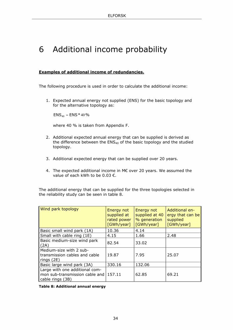
6 Additional income probability

Examples of additional income of redundancies.

The following procedure is used in order to calculate the additional income:

1. Expected annual energy not supplied (ENS) for the basic topology and for the alternative topology as:

where 40 % is taken from Appendix F.

%*ENSENS 4040 =

2. Additional expected annual energy that can be supplied is derived as the difference between the ENS40 of the basic topology and the studied topology.

3. Additional expected energy that can be supplied over 20 years.

4. The expected additional income in M€ over 20 years. We assumed the value of each kWh to be 0.03 €.

The additional energy that can be supplied for the three topologies selected in the reliability study can be seen in table 8.

Wind park topology Energy not supplied at rated power [GWh/year]

Energy not supplied at 40 % generation [GWh/year]

Additional en-ergy that can be supplied [GWh/year]

Basic small wind park (1A) 10.36 4.14 Small with cable ring (1E) 4.15 1.66 2.48 Basic medium-size wind park (2A)

82.54 33.02

Medium-size with 2 sub-transmission cables and cable rings (2E)

19.87 7.95 25.07

Basic large wind park (3A) 330.16 132.06 Large with one additional com-mon sub-transmission cable and cable rings (3B)

157.11 62.85 69.21

Table 8: Additional annual energy

34

ELFORSK

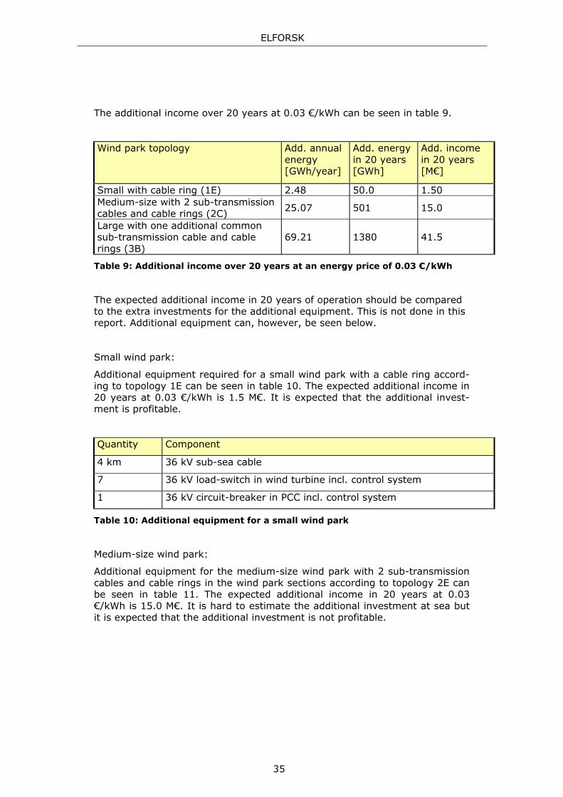
The additional income over 20 years at 0.03 €/kWh can be seen in table 9.

Wind park topology Add. annual energy [GWh/year]

Add. energy in 20 years [GWh]

Add. income in 20 years [M€]

Small with cable ring (1E) 2.48 50.0 1.50 Medium-size with 2 sub-transmission cables and cable rings (2C)

25.07 501 15.0

Large with one additional common sub-transmission cable and cable rings (3B)

69.21 1380 41.5

Table 9: Additional income over 20 years at an energy price of 0.03 €/kWh

The expected additional income in 20 years of operation should be compared to the extra investments for the additional equipment. This is not done in this report. Additional equipment can, however, be seen below.

Small wind park:

Additional equipment required for a small wind park with a cable ring accord-ing to topology 1E can be seen in table 10. The expected additional income in 20 years at 0.03 €/kWh is 1.5 M€. It is expected that the additional invest-ment is profitable.

Quantity Component

4 km 36 kV sub-sea cable

7 36 kV load-switch in wind turbine incl. control system

1 36 kV circuit-breaker in PCC incl. control system

Table 10: Additional equipment for a small wind park

Medium-size wind park:

Additional equipment for the medium-size wind park with 2 sub-transmission cables and cable rings in the wind park sections according to topology 2E can be seen in table 11. The expected additional income in 20 years at 0.03 €/kWh is 15.0 M€. It is hard to estimate the additional investment at sea but it is expected that the additional investment is not profitable.

35

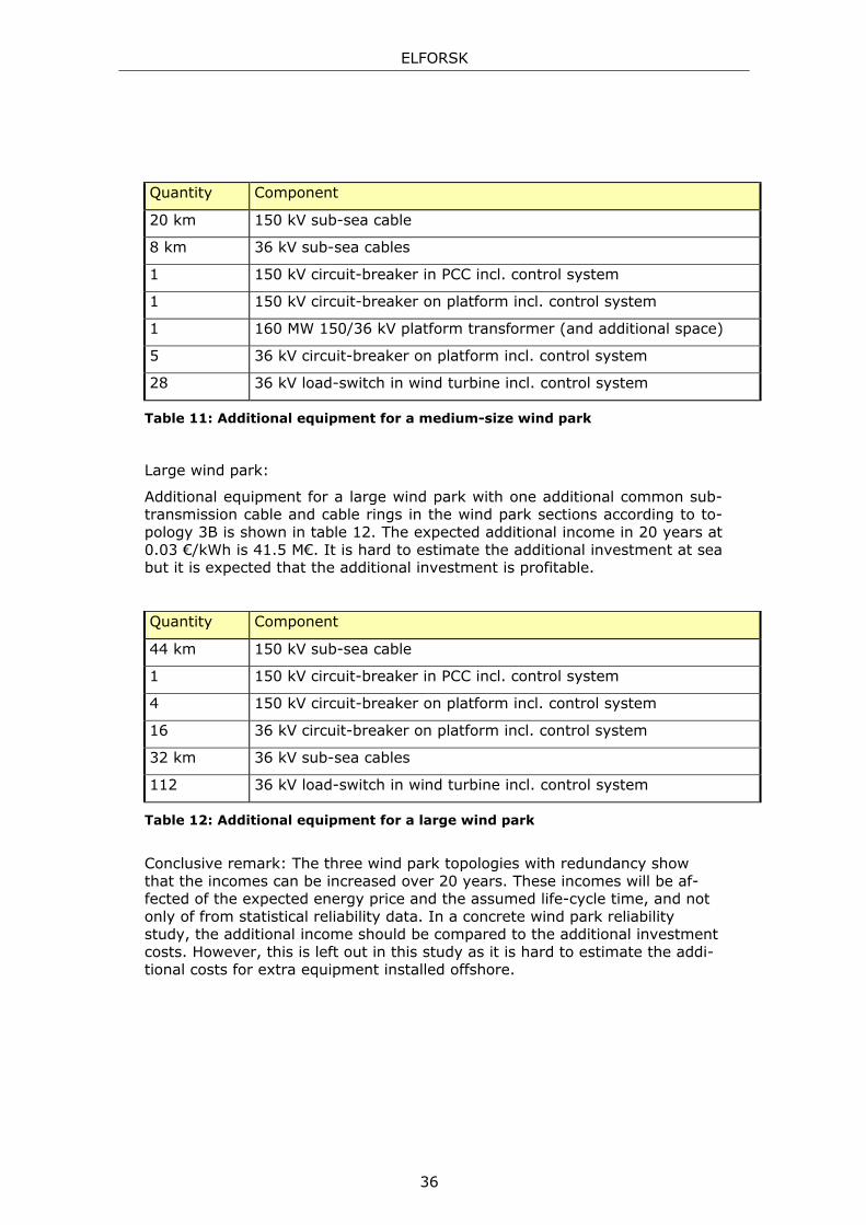
ELFORSK

Quantity Component


8 km 36 kV sub-sea cables


1 150 kV circuit-breaker on platform incl. control system

1 160 MW 150/36 kV platform transformer (and additional space)



Table 11: Additional equipment for a medium-size wind park

Large wind park:

Additional equipment for a large wind park with one additional common sub-transmission cable and cable rings in the wind park sections according to to-pology 3B is shown in table 12. The expected additional income in 20 years at 0.03 €/kWh is 41.5 M€. It is hard to estimate the additional investment at sea but it is expected that the additional investment is profitable.

Quantity Component





32 km 36 kV sub-sea cables


Table 12: Additional equipment for a large wind park

Conclusive remark: The three wind park topologies with redundancy show that the incomes can be increased over 20 years. These incomes will be af-fected of the expected energy price and the assumed life-cycle time, and not only of from statistical reliability data. In a concrete wind park reliability study, the additional income should be compared to the additional investment costs. However, this is left out in this study as it is hard to estimate the addi-tional costs for extra equipment installed offshore.

36

ELFORSK

7 Conclusions

In this report a reliability optimization method is presented that may be used for investment decisions concerning sub-sea cable systems of offshore wind parks. The method is based on reliability computations in different designs of the collection grid for the wind park. The method is using reliability data of involved components such as failure rates, repair times and switching times. The method consists of three distinctive stages:

• In the first stage, the expected annual energy not supplied is derived for the basic configuration. In principle, the basic configuration can be any configuration, but a configuration without any redundancy could be an appropriate choice. The expected annual energy not supplied is calculated.

• In the second stage, redundancy is built into the collection grid. The choice of redundancy is based on the contribution of each component to the expected annual energy not supplied. The difference between the energy not supplied in the basic and in the new configuration is the additional energy that can be supplied.

• The third stage is an economical evaluation where the additional en-ergy that can be supplied is converted to additional income per year or over a whole life-cycle. At this stage the method is using assumptions regarding the energy price and the number of years in a life-cycle.

The method can be used for comparison of different configurations or for comparison of additional income versus additional investment in redundancy. The method can also be used to estimate the expected annual energy produc-tion of an existing wind park or an existing design.

The method is applied for case studies of three different sizes of offshore wind parks: small; medium-size; and large. A typical topology without redundancy for each size is used as basic configuration. The experiences from the case studies can be summarized in the following conclusions:

• The main contribution to the expected annual energy not supplied is due to the long repair time of components at an offshore location.

• Redundancy is introduced in the form of spare capacity in sub-sea ca-bles and additional cables and transformers.

• Two levels of redundancy should be distinguished based on the type of switchgear used. Remote-controlled load-switches in combination with remote indication of faulted segment will result in a restoration time

37

ELFORSK

between several minutes and one hour. Circuit-breakers with appropri-ate protection equipment will reduce the number of interruptions.

• The additional gain of installing circuit-breakers is limited whereas the costs are typically very high. The costs may include the costs of switchgear able to withstand the higher fault currents.

• The gain of installing remote-controlled load-switches is significant as it reduces the duration of a production stoppage from several weeks or months to one hour or less.

• There is an optimal number of load-switches, above which additional ones only increase costs and complexity without significant further gains in expected annual energy production.

The method described in this report is a probabilistic method, which is inher-ently associated with uncertainty. Some care should be taken in comparing rather accurately known investment costs with uncertain gain in annual pro-duction. A small difference in total costs between two design alternatives should not be seen as significant and a base for an investment decision. There are, however, no general rules for how to handle this and a further discussion on this is beyond the scope of this report.

A change in input parameters (failure rate, expected repair time, investment costs, value of non-delivered energy) may impact the preferred design under the method described in this report. As several of the input parameters are in itself uncertain, this would introduce an additional uncertainty in the final de-cision. However, it is generally accepted in power system reliability that the outcome of the comparison is not impacted when the most-likely value is used for all input parameters and when the difference between the design is not too small.

38

ELFORSK

8 References

[1] ”Reliability of Collection Grids for Large Offshore Wind Parks”. A. Sannino, H. Breder, E.K. Nielsen. PMAPS 2006.

[2] ”Collection Grid Topologies for Off-shore Wind Parks”. B. Frankén, H. Bre-der, M. Dahlgren, E.K. Nielsen. CIRED, 6-9 June, 2005.

[3] ”Literature search for Reliability Data of Components in electric Distribu-tion Networks”. M.H.J. Bollen. August 1993.

[4] ”Electrical System Designs for the Proposed 1 GW Beatrice Offshore Wind-farm”. G.W. Ault, S. Gair, J.R. McDonald. Fifth International workshop on Large-Scale Integration of Wind Power and Transmission Networks for Offshore Wind Farms. 7-8 april 2005.

[5] ”Economic Comparison of HVAC and HVDC Solutions for Large Offshore Windfarms under Special Consideration of Reliability”. L. Lazaridis, T. Ackermann. Fifth International workshop on Large-Scale Integration of Wind Power and Transmission Networks for Offshore Wind Farms. 7-8 april 2005.

[6] ”www.vattenfall.se”

[7] ”www.vattenfall.de” [8] ”www.vestas.com”

[9] ”www.offshore-wind.de” [10] ”www.uni-saarland.de”

[11] ”www.elsamkraft.com” [12] ”www.kentishflats.co.uk”

[13] ”www.neplan.ch”

[14] ”Vindforsk Nyhetsbrev 2, 2006” [15] ”Method for assessing offshore wind farm cable reliabity incorporating

cost effectiveness of redundancy”. G. Takoudis, G. Ault, S. Gair, J. McDonald. International Workshop on Large-Scale Intergration of Wind Power and Transmission Networks for Offshore Wind Farms, 7-8 April, 2005, Glasgow, Scotland.

[16] “Reliability Evaluation of Power Systems”. R. Billinton, R.N. Allan. ISBN 0-273-08485-2 1984.

Appendix Appendix A: Failure rate Appendix B: Reparation time Appendix C: Switching time Appendix D: Electrical data of sub-sea cables Appendix E: Example of Neplan Reliability Results Appendix F: Average production level

39

ELFORSK

Appendix A: Reliability data – Failure rates (�)

In the following table the failure rate data is presented. These data has been used in the Neplan reliability calculations for the different studied topologies of the collection grids.

Component Failure rate

[failure/year]

Sub-sea cables (150 kV) 0.008 [failure /year,km]

Sub-sea cables (36 kV) 0.008 [failure /year,km]

Platform transformers (160 MW, 150 kV) 0.020

Circuit-breakers (36 kV on land) 0.024

Circuit-breakers (36 kV on platform) 0.024

Circuit-breakers (36 kV in wind turbine) 0.024

Circuit-breakers (150 kV on land) 0.032

Circuit-breakers (150 kV on platform) 0.032

Disconnectors (36 kV on land) 0.0024

Disconnectors (36 kV on platform) 0.0024

Disconnectors (150 kV on land) 0.012

Disconnectors (150 kV on platform) 0.012

Load-switches (36 kV in wind turbine) 0.020

Busbars (36 kV on offshore platform) 0.004

Busbars (150 kV on offshore platform) 0.020

Table 13: Failure rates used in the study

40

ELFORSK

Appendix B: Reliability data – Reparation times (MTTR)

In the following table the reparation time data is presented.

Component Repair time

[h]

Comment

Sub-sea cables (150 kV) 720 2)

Sub-sea cables (36 kV) 2160 3)

Platform transformers (160 MW, 150 kV) 4320 4)

Circuit-breakers (36 kV on land) 4 1)

Circuit-breakers (36 kV on platform) 720 2)

Circuit-breakers (36 kV in wind turbine) 2160 3)

Circuit-breakers (150 kV on land) 4 1)

Circuit-breakers (150 kV on platform) 720 2)

Disconnectors (36 kV on land) 4 1)

Disconnectors (36 kV on platform) 720 2)

Disconnectors (150 kV on land) 12 1)

Disconnectors (150 kV on platform) 720 2)

Load-switches (36 kV in wind turbine) 2160 3)

Busbars (36 kV on offshore platform) 720 2)

Busbars (150 kV on offshore platform) 720 2)

Table 14: Repair times used in the study

1) Based on statistic information for distribution and industrial systems. 2) Based on assumption of longer repair times for offshore equipment in this study. 3) Based on additional delay times due to waiting times for reparation during the winter seasons in this study. 4) Based on delay times due to replacement of platform transformers which require lifting, transportation and spare units.

41

ELFORSK

Appendix C: Reliability data – Switching times (MTTS)

The switching time data is presented in the table below.

Component Switching time

[min]

Circuit-breakers (all) 20

Disconnectors (all) 20

Load-switches in wind turbine 20

Table 15: Switching times used in the study

42

ELFORSK

Appendix D: Electrical data of sub-sea cables

The following electrical data is used for the sub-sea cables.

Voltage [kV]

Cable area [mm2]

Resistance

[ohm/km]

Reactance

[ohm/km]

Capacitance

[µF/km]

Current limit

[A] ([MW])

36 300 0.056 0.110 0.200 355 (20)

36 600 0.028 0.110 0.200 710 (40)

36 1200 0.014 0.110 0.200 1420 (80)

150 600 0.028 0.110 0.200 710 (160)

Table 16: Electrical cable data used in the study

43

ELFORSK

Appendix E: Example of Neplan Reliability Results

The different topologies of the collection grids of the offshore wind parks have been executed in the Reliability module of Neplan software package. The evaluation results of the processing of the basic topology 1A are presented in tables 17 and 18.

Topology 1A

Index Unit Value Description ASAI % 97.040 Average service availability index λ Failure/year 0.149 Average failure rate r h 1742.7 Average outage time U min/year 15558.9 Average annual outage time ENS MWh/year 10362.2 Annual energy not supplied

Table 17: Neplan results of total topology 1A

Name Type λ [1/year] r [h] U [min/year] ENS [MWh/year]*** Total *** 0.149 1742.7 15558.9 10362.2 FeederCable Cable 0.032 2160.0 4147.2 2762.0 Intercable-1 Cable 0.008 2160.0 1036.8 690.5 Intercable-2 Cable 0.008 2160.0 1036.8 690.5 Intercable-3 Cable 0.008 2160.0 1036.8 690.5 Intercable-4 Cable 0.008 2160.0 1036.8 690.5 Intercable-5 Cable 0.008 2160.0 1036.8 690.5 Intercable-6 Cable 0.008 2160.0 1036.8 690.5 Intercable-7 Cable 0.008 2160.0 1036.8 690.5 Intercable-8 Cable 0.008 2160.0 1036.8 690.5 Intercable-9 Cable 0.008 2160.0 1036.8 690.5 Intercable-10 Cable 0.008 2160.0 1036.8 690.5 Intercable-11 Cable 0.008 2160.0 1036.8 690.5 Circuit-Breaker Circuit breaker 0.024 4.0 5.760 3.836 Disconnector-2 Disconnector 0.002 4.0 0.576 0.384 Disconnector-1 Disconnector 0.002 4.0 0.576 0.384

Table 18: Neplan results of total topology 1A and of individual components

44

ELFORSK

Appendix F: Average production level

The value of one hour of generation depends on many factors that are un-known at this stage of the study, e.g. wind speed, electricity price, availability of balancing power within the company. etc.

In order to get an estimate of the loss in income to the unavailability of the wind park, an estimation has been made of the average value of one hour of generation.

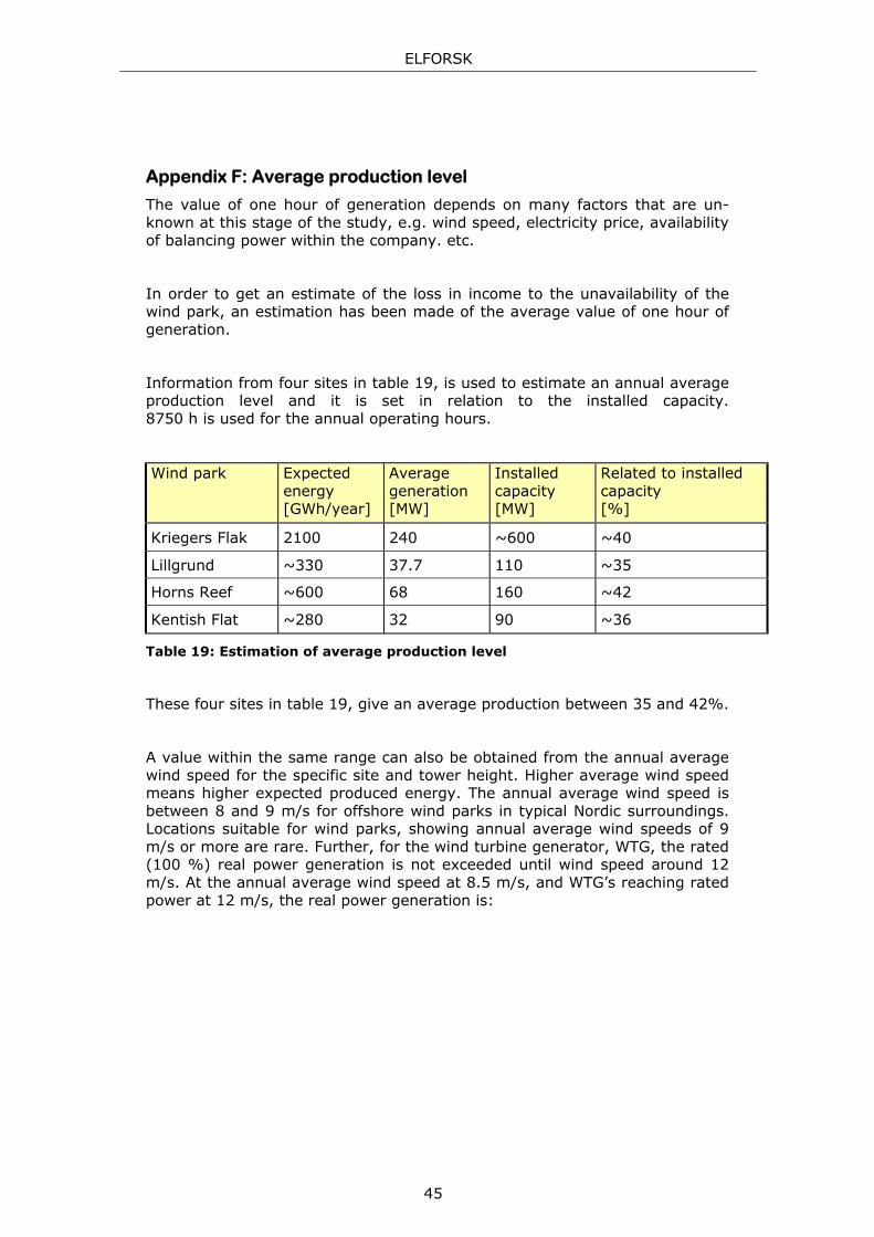
Information from four sites in table 19, is used to estimate an annual average production level and it is set in relation to the installed capacity. 8750 h is used for the annual operating hours.

Wind park Expected energy [GWh/year]

Average generation [MW]

Installed capacity [MW]

Related to installed capacity [%]

Kriegers Flak 2100 240 ~600 ~40

Lillgrund ~330 37.7 110 ~35

Horns Reef ~600 68 160 ~42

Kentish Flat ~280 32 90 ~36

Table 19: Estimation of average production level

These four sites in table 19, give an average production between 35 and 42%.

A value within the same range can also be obtained from the annual average wind speed for the specific site and tower height. Higher average wind speed means higher expected produced energy. The annual average wind speed is between 8 and 9 m/s for offshore wind parks in typical Nordic surroundings. Locations suitable for wind parks, showing annual average wind speeds of 9 m/s or more are rare. Further, for the wind turbine generator, WTG, the rated (100 %) real power generation is not exceeded until wind speed around 12 m/s. At the annual average wind speed at 8.5 m/s, and WTG’s reaching rated power at 12 m/s, the real power generation is:

45

ELFORSK

( )

conditionsnominalatspeedwindisvspeedwindactualisv

generationnominalisPgenerationactualisPwhere

P*.P*,

P*vv

P

vfPands/mvatPP

n

n

nnnn

nn

36012

58

1233

3

=⎟⎠

⎞⎜⎝

⎛=⎟⎟⎠

⎞⎜⎜⎝

⎛=

=>===

This value, which is 36 % of nominal power, is within the range derived be-fore. From this we conclude that an annual average wind speed will result in an average real power generation per hour which is somewhere around 36 %. The distribution of the wind speed at the site is needed for a more accurate calculation.

In the study, 40 % is used as an approximate value.

46

reliability study: analysis of electrical systems within offshore wind

Documents