reliability based durability assessment of gfrp bars … · reliability-based durability assessment...
TRANSCRIPT

RELIABILITY-BASED DURABILITY ASSESSMENT OF GFRP BARS FOR REINFORCED CONCRETE
Nicole D. Jackson
Thesis submitted to the Faculty of the Virginia Polytechnic Institute and State University
in partial fulfillment of the requirements for the degree of
Master of Science in
Engineering Mechanics
Scott W. Case, Chair John J. Lesko
Carin L. Roberts-Wollmann
12 November 2007 Blacksburg, Virginia
Keywords: Glass fiber reinforced polymer (GFRP), Monte Carlo, Concrete, Reliability
Copyright 2007 by Nicole D. Jackson

RELIABILITY-BASED DURABILITY ASSESSMENT OF GFRP BARS FOR
REINFORCED CONCRETE
Nicole D. Jackson
ABSTRACT
The American Concrete Institute (ACI) has developed guidelines for the design of fiber
reinforced polymer (FRP) reinforced concrete structures. Current guidelines require the application
of environmental and flexural strength reduction factors, which have minimal experimental
validation. Our goal in this research is the development of a Monte Carlo simulation to assess the
durability of glass fiber reinforced polymer (GFRP) reinforced concrete designed for flexure. The
results of this simulation can be used to determine appropriate flexural strength reduction factors.
Prior to conducting the simulation, long-term GFRP tensile strength values needed to be
ascertained. Existing FRP tensile strength models are limited to short-term predictions. This study
successfully developed a power law based-FRP tensile strength retention model using currently
available tensile strength data for GFRP exposed to variable temperatures and relative humidity.
GFRP tensile strength retention results are projected at 0, 1, 3, 10, 30, and 60-year intervals. The
Monte Carlo simulation technique is then used to assess the influence beam geometry, concrete
strength, fractions of balanced reinforcement ratio, reinforcing bar tensile strength, and
environmental reduction factors on the flexural capacity of GFRP reinforced concrete beams.
Reliability analysis was successfully used to determine an environmental reduction factor of
0.5 for concrete exposed to earth and weather. For simulations with higher GFRP bar tensile
strength as well as larger beam geometry and fractions of the balanced reinforcement ratio, larger
moment capacities were produced. A strength reduction factor of approximately 0.8 is calculated for
all fractions of balanced reinforcement ratio. The inclusion of more long-term moisture data for
GFRP is necessary to develop a more cohesive tensile strength retention model. It is also
recommended that longer life cycles of the GFRP reinforced concrete beams be simulated.
This research was conducted thanks to support from the National Science Foundation Division of Graduate Education’s Interdisciplinary Graduate Education Research and Traineeship (Award # DGE-0114342) Note: The opinions expressed herein are the views of the authors and should not be interpreted as the views of the National Science Foundation.

iii
ACKNOWLEDGEMENTS
I would like to thank my advisor and committee chairperson, Dr. Scott Case, for his
guidance and advice. Without his assistance, much of the thesis would not be possible. I would also
like to thank Dr. Carin Roberts-Wollmann and Dr. Jack Lesko for serving on my thesis committee.
Much of my time would not have transpired as smoothly without the endless help of Beverly
Williams and Joyce Smith. Many thanks go out to other the students in the Materials Response
Group. A special thanks goes out to Dr. Christine Fiori and Dr. John Popovics, who were my
undergraduate mentors and opened my eyes to the wonderful world of research. I wouldn’t be here
without either one of you.

iv
TABLE OF CONTENTS
LIST OF FIGURES..........................................................................................................................................................VI LIST OF TABLES.........................................................................................................................................................VIII CHAPTER 1 INTRODUCTION...................................................................................................................................... 1
1.1 BACKGROUND ............................................................................................................................................................ 1 1.2 OBJECTIVES ................................................................................................................................................................ 2
1.2.1 Primary Goal ..................................................................................................................................................... 2 1.2.2 Secondary Goals................................................................................................................................................ 2
CHAPTER 2 LITERATURE REVIEW ......................................................................................................................... 3 2.1 GENERAL .................................................................................................................................................................... 3 2.2 APPLICATIONS FOR CIVIL INFRASTRUCTURE............................................................................................................. 3 2.3 LIFE CYCLE COSTS OF FRP BRIDGE DECKS ............................................................................................................... 4 2.4 DURABILITY OF GFRP ............................................................................................................................................... 5 2.5 DEGRADATION MECHANISMS .................................................................................................................................... 6
2.5.1 Moisture degradation........................................................................................................................................ 6 2.5.2 Hygrothermal effects ......................................................................................................................................... 8 2.5.3 Alkali attack ....................................................................................................................................................... 9
2.6 DESIGN CODE PROVISIONS ........................................................................................................................................ 9 2.6.1 Flexural strength of GFRP ............................................................................................................................... 9 2.6.2 Environmental reduction factors.................................................................................................................... 11 2.6.3 Application of load and resistance factor design (LRFD) to FRP............................................................... 14
2.7 FRP TENSILE STRENGTH PREDICTIONS .................................................................................................................. 14 2.7.1 Regression-based tensile strength prediction................................................................................................ 15 2.7.2 Diffusion based tensile strength prediction ................................................................................................... 15 2.7.3 Litherland Method........................................................................................................................................... 16
2.8 EXPERIMENTAL STRENGTH DEGRADATION DATA OF GFRP BARS......................................................................... 16 2.8.1 Experimental Procedure ................................................................................................................................. 17
2.8.1.1 Conditioning of tensile test specimens .......................................................................................................................17 2.8.1.2 Tensile Testing Procedure...........................................................................................................................................18 2.8.1.3 Moisture absorption experiments................................................................................................................................20
2.8.2 Experimental Results....................................................................................................................................... 21 2.8.2.1 Tensile test results........................................................................................................................................................21 2.8.2.2 Moisture absorption results .........................................................................................................................................25
2.9 CONCLUSION ............................................................................................................................................................ 26 CHAPTER 3 COMPUTATIONAL PROCEDURE................................................................................................... 28
3.1 TENSILE STRENGTH RETENTION MODELS .............................................................................................................. 28 3.1.1 Existing Tensile Strength Models ................................................................................................................... 28
3.1.1.1 Durability prediction via short-term accelerated aging .............................................................................................28 3.1.1.2 Deterioration prediction from alkali attack ................................................................................................................34
3.1.2 Modeling existing tensile data ........................................................................................................................ 38 3.1.2.1 Tensile strength with variable conditioning temperatures ........................................................................................39 3.1.2.2 Tensile strength with variable relative humidity conditions .....................................................................................43 3.1.2.3 Tensile strength with combined relative humidity and temperature effects ............................................................49
3.2 MONTE CARLO SIMULATIONS ................................................................................................................................. 55 3.2.1 Random number generation ........................................................................................................................... 56 3.2.2 Parameterized elements .................................................................................................................................. 56
3.2.2.1 GFRP tensile strength..................................................................................................................................................56 3.2.2.2 Concrete Strength ........................................................................................................................................................58 3.2.2.3 Concrete beam and slab dimensions...........................................................................................................................59 3.2.2.4 Summary of parameterized elements .........................................................................................................................60
3.2.3 Flexural design of FRP reinforced concrete beams ..................................................................................... 61

v
3.2.3.1 Input values ..................................................................................................................................................................61 3.2.3.2 GFRP reinforcement....................................................................................................................................................62 3.2.3.3 Strain-compatibility analysis.......................................................................................................................................65 3.2.3.4 Nominal flexural strength............................................................................................................................................66
3.3 RELIABILITY ASSESSMENT....................................................................................................................................... 67 3.3.1 Weibull distribution models ............................................................................................................................ 68
3.3.1.1 Background on the Weibull distribution ....................................................................................................................68 3.3.1.2 Methods for estimating parameters ............................................................................................................................70 3.3.1.3 Development of confidence intervals .........................................................................................................................71
3.3.2 Determination of environmental reduction factors ....................................................................................... 76 3.3.2.1 Monte Carlo simulations for bar strength ..................................................................................................................76 3.3.2.2 Computational procedure ............................................................................................................................................77
3.3.3 Determination of strength reduction factors ................................................................................................. 79 CHAPTER 4 RESULTS .................................................................................................................................................. 81
4.1 INTRODUCTION......................................................................................................................................................... 81 4.2 ENVIRONMENTAL REDUCTION FACTORS ................................................................................................................ 81 4.3 MONTE CARLO SIMULATION RESULTS .................................................................................................................... 85
4.3.1.1 Effect of environmental reduction factors..................................................................................................................86 4.3.1.2 Effect of beam geometry .............................................................................................................................................90 4.3.1.3 Effect of concrete strength ..........................................................................................................................................97
4.4 STRENGTH REDUCTION FACTORS........................................................................................................................... 100 CHAPTER 5 CONCLUSIONS .................................................................................................................................... 106
5.1 INTRODUCTION....................................................................................................................................................... 106 5.2 CONCLUSIONS ........................................................................................................................................................ 106
5.2.1 Environmental reduction factors.................................................................................................................. 106 5.2.2 Monte Carlo simulation parameters ............................................................................................................ 106 5.2.3 Strength reduction factors ............................................................................................................................ 107
5.3 RECOMMENDATIONS FOR FUTURE WORK.............................................................................................................. 107 REFERENCES................................................................................................................................................................ 109

vi
LIST OF FIGURES
Figure 2-1: Primary and secondary effects of moisture absorption on composite materials. ...................................... 8 Figure 2-2: Side and full view schematics of the conditioning tank used by Bhise for short-term immersion testing of GFRP bars. ........................................................................................................................................................................ 18 Figure 2-3: Layout of the specimen ready for tensile test. Anchors are used to provide better gripping in the UTM and are applied after the specimen is removed from the solution................................................................................... 19 Figure 3-1: Tensile strength retention of GFRP1 bars exposed to Solution 1 at 20, 40, and 60°C [20]..................... 30 Figure 3-2: Tensile strength retention versus exposure time for GFRP1 bars [20]...................................................... 33 Figure 3-3: Tensile strength retention versus long-term exposure time for GFRP1 bars............................................. 34 Figure 3-4: GFRP tensile strength results for specimens subject to accelerated aging at 40 C with a 1.0 mol/l aqueous NaOH solution. [21]............................................................................................................................................ 35 Figure 3-5: Experimental and projected tensile strength results for GFRP bars.......................................................... 37 Figure 3-6: Predicted tensile strength retention for GFRP based on a diffusion model for strength retention. ......... 38 Figure 3-7: Temperature-based time shift factors for GFRP versus exposure temperature. Note that the reference temperature is 30 °C........................................................................................................................................................... 40 Figure 3-8: Tensile strength retention of GFRP bars subject to variable temperatures after the temperature-based shift factors have been applied. ......................................................................................................................................... 41 Figure 3-9: Tensile strength retention versus shifted time for GFRP bars subject to variable temperatures. The power-law model for GFRP tensile strength retention is overlaid. ................................................................................ 42 Figure 3-10: Effect of a variable moisture absorbing condition on the tensile strength of GFRP plates as a function of exposure time. [24] ........................................................................................................................................................ 45 Figure 3-11: Relative humidity based time shift factors for GFRP versus exposure relative humidity. Note that the reference relative humidity is 30%.................................................................................................................................... 46 Figure 3-12: Tensile strength retention of GFRP plates subject to variable relative humidity after the relative humidity-based shift factors have been applied................................................................................................................ 47 Figure 3-13: Tensile strength retention versus shifted time for GFRP plates subject to variable relative humidity. The power-law model for the GFRP tensile strength retention is overlaid. ................................................................... 48 Figure 3-14: Natural logarithm of temperature-based shift factors versus the inverse of temperature. Note that the reference temperature is 30 °C.......................................................................................................................................... 51 Figure 3-15: Natural logarithm of relative humidity-based shift factors versus difference in relative humidity. Note that the reference relative humidity is 30%. ..................................................................................................................... 52 Figure 3-16: Tensile strength retention versus shifted time for GFRP composites with superimposed temperature and relative humidity effects. The power-law model for the GFRP tensile strength retention is overlaid................... 54 Figure 3-17: Concrete beam with dimensions.................................................................................................................. 59 Figure 3-18: The Weibull probability density function [29] ........................................................................................... 69 Figure 4-1: Comparison of Weibull-based moment capacities for Member A using projected 0 and 60 year GFRP tensile strength values ........................................................................................................................................................ 82 Figure 4-2: Comparison of Weibull-based moment capacities for Member A using both 0 year and 60-year projected GFRP tensile strength values. The 0 year revised and ACI moment capacities have incorporated environmental reduction factors of 0.5 and 0.7, respectively, to the 0-year GFRP tensile strength. ........................... 83 Figure 4-3: Environmental reduction factors for Member A designed with 4000 psi concrete as a function of time. 85

vii
Figure 4-4: Weibull-based nominal flexural strength as a function of environmental reduction factor for Member A designed with 4000 psi concrete at balanced reinforcement ratio conditions. .............................................................. 87 Figure 4-5: Percentage of simulations occurring below the nominal flexural strength for GFRP reinforced concrete members as a function of the environmental reduction factor for Member A designed with 4000 psi concrete and balanced reinforcement ratio conditions. ......................................................................................................................... 88 Figure 4-6: Percentage of failures out of 10,00 simulations due to FRP bar rupture for Member A designed with 4000 psi concrete and balanced reinforcement ratio conditions. ................................................................................... 89 Figure 4-7: Total GFRP reinforcing bar area for Member A with respect to varying concrete strength and fractions of balanced reinforcement ratio. ....................................................................................................................................... 91 Figure 4-8: Total GFRP reinforcing bar area for Member C with respect to varying concrete strength and fraction of balanced reinforcement ratio. ....................................................................................................................................... 92 Figure 4-9: Nominal flexural strength for GFRP reinforced concrete members with respect to total GFRP reinforcing bar area for Members A and C. The illustrations shown are used to draw contrast to different beam geometries of the different members.................................................................................................................................. 93 Figure 4-10: Nominal flexural strength for GFRP reinforced concrete Member A with respect to environmental reduction factor and fraction of balanced reinforcement ratio. The member was designed with 4000 psi concrete. . 94 Figure 4-11: Nominal flexural strength for GFRP reinforced concrete member C with respect to environmental reduction factor and fraction of balanced reinforcement ratio. The member was designed with 4000 psi concrete. . 95 Figure 4-12: Percentage of simulation failures due to FRP bar rupture for Member A designed with 4000 psi concrete with respect to fractions of balanced reinforcement ration and environmental reduction factor. All environmental reduction factors were subject to 100% FRP bar rupture failure except for factors of 0.8 and 1.0. . 96 Figure 4-13: Percentage of simulation failures due to FRP bar rupture for Member C design with 4000 psi concrete and with respect to fractions of balanced reinforcement ration and environmental reduction factor. All environmental reduction factors were subject to 100% FRP bar rupture failure except for the factors of 0.8 and 1.0............................................................................................................................................................................................... 97 Figure 4-14: Nominal flexural strength for GFRP reinforced concrete Member A with respect to fractions of balanced reinforcement ratio and concrete strength. ...................................................................................................... 98 Figure 4-15: Percentage of simulation failures due to bar rupture with respect to fraction of balanced reinforcement ratio for Member A designed with 4000, 5000, and 6000 psi concrete. Values of 100% indicate all 10,000 simulations experienced this failure mode........................................................................................................................ 99 Figure 4-16: ACI-based flexural strength reduction factors with respect to fractions of the balanced reinforcement ratio. 1.5 and 1.6 times the balanced reinforcement ratio are also presented to verify the strength reduction factor of 0.65. Neither values were directly employed in the Monte Carlo simulations. ............................................................ 101 Figure 4-17: Flexural strength reduction factors based on Ellingwood with β = 3.5 for Member A designed with 4000 psi concrete. Similar results were reported throughout the simulations. ............................................................ 103 Figure 4-18: Flexural strength reduction factors based on Ellingwood with β = 4.0 for Member A designed with 4000 psi concrete. As with the β = 3.5, similar results were recorded amongst all simulations. ............................... 104 Figure 4-19: Comparison of flexural strength reduction factors for all methods under consideration. The current values provided by ACI yield the most conservative design estimates for the moment capacity of GFRP reinforced concrete beams. ................................................................................................................................................................ 105

viii
LIST OF TABLES
Table 2-1: Life-cycle costs for traditional steel reinforced and FRP reinforced concrete bridge decks. The FRP premium represents the difference in cost estimates between the two bridges. Note that costs in parentheses indicate negative dollar amounts. ...................................................................................................................................................... 4 Table 2-2: Partial safety factors proposed for fiber-reinforced polymer reinforced concrete structures for usage in EUROCODE 8 ................................................................................................................................................................... 11 Table 2-3: Environmental reduction factor for various fibers and exposure conditions per ACI 440.1R-06 ............. 12 Table 2-4: Comparison of the existing code specified and experimentally determined environmental reduction factors for carbon, glass, and aramid fiber reinforced concrete structures. The highest, median, and lowest values are reported. ....................................................................................................................................................................... 13 Table 2-5: Reduction factors for GFRP bars suggested by the American Concrete Institute, Canadian Standards Association, and the Japanese Society of Civil Engineers. ............................................................................................ 14 Table 2-6: Tensile strength and modulus of elasticity for plain #3 GFRP bars. Values based on the nominal and measured cross-sectional areas of the bars are reported. ............................................................................................... 19 Table 2-7: Tensile strength and modulus of elasticity for incased but unconditioned bars #3 GFRP bars. Values based on the nominal and measured cross-sectional areas of the bars are reported.................................................... 20 Table 2-8: Tensile strength of #3 GFRP bars subject to 30, 45, and 57 °C temperatures for 10, 30, 60, 90, and 180 days. ..................................................................................................................................................................................... 22 Table 2-9: Average tensile strength and coefficient of variation of #3 GFRP bars subject to 30, 45, and 57°C temperatures for 10, 30, 60, 90, and 180 days. ................................................................................................................ 23 Table 2-10: Modulus of elasticity for #3 GFRP bars subject to 30, 45, and 57°C temperatures for 10, 30, 60, 90, and 180 days............................................................................................................................................................................... 24 Table 2-11: Average modulus of elasticity and coefficient of variation of #3 GFRP bars subject to 30, 45, and 57°C temperatures for 10, 30, 60, 90, and 180 days. ................................................................................................................ 25 Table 2-12: Moisture absorption data based on weight gain percentages for #3 GFRP specimens immersed in limewater solution. ............................................................................................................................................................. 25 Table 2-13: Maximum moisture and diffusion for #3 GFRP bars immersed in a limewater solution at 30, 45, 57°C............................................................................................................................................................................................... 26 Table 2-14: Arrhenius analysis results based on a Fickian curve fit with respect to immersion temperatures of 30, 45, and 57°C. ...................................................................................................................................................................... 26 Table 3-1: Chemical compositions of simulated concrete pore solutions. Solution 1 has a pH of 13.6, and Solution 2 has a pH value of 12.7, which closely resembles the pore environment found in typical high performance concretes. .............................................................................................................................................................................................. 29 Table 3-2: Short-term accelerated aging test matrix for GFRP bars immersed in concrete pore solutions. [20] ...... 29 Table 3-3: Coefficients of regression equations for GFRP bar tensile strength retention immersed in both concrete pore solutions 1 and 2. [20]............................................................................................................................................... 31 Table 3-4: Coefficient of Regression Equations for Arrhenius Plots immersed in both concrete pore solutions 1 and 2 [20] ................................................................................................................................................................................... 32 Table 3-5: Values for Acceleration Factors [20] ............................................................................................................. 32 Table 3-6: Temperature-based shift factors for GFRP tensile strength retention based on a reference temperature of 30°C..................................................................................................................................................................................... 39 Table 3-7: Predicted long-term tensile strength retention based on variable temperature data .................................. 43

ix
Table 3-8: GFRP tensile strength retention results for variable humidity ..................................................................... 44 Table 3-9: Relative humidity-based shift factors for GFRP tensile strength retention based on a reference relative humidity of 30%. ................................................................................................................................................................. 46 Table 3-10: Predicted long-term tensile strength retention based on variable relative humidity data ........................ 49 Table 3-11: Predicted long-term tensile strength retention for GFRP based on superimposed relative humidity and temperature data................................................................................................................................................................. 55 Table 3-12: Physical properties of #3 Aslan 100 GFRP Rebar by Hughes Brothers .................................................... 57 Table 3-13: Statistical and mechanical properties of GFRP bars ................................................................................. 58 Table 3-14: Statistical parameters of ordinary ready-mix concrete [26] ...................................................................... 59 Table 3-15: Statistical parameters of dimensional variables .......................................................................................... 60 Table 3-16: Statistical properties of variables involved in this study ............................................................................. 61 Table 3-17: Member dimensions ....................................................................................................................................... 62 Table 3-18: Taxonomy for Weibull Models. ..................................................................................................................... 70


1
CHAPTER 1 Introduction
1.1 Background
Steel bars are the predominant form of reinforcement for concrete structures. The natural
porosity of concrete and exposure to harsh environments causes steel to be highly susceptible to
corrosion. The limited long-term durability and high cost of maintenance of steel rebar has lead to
increased interest in other reinforcing materials, particularly fiber reinforced polymers (FRP).
First-generation FRP materials where characterized by poor stiffness and tensile properties.
Early FRP reinforced concrete design guidelines lead to conservative estimates of environmental and
strength reduction factors. These factors have limited empirical basis and are generally selected by
committee consensus. A greater understanding of durability mechanisms and improved
manufacturing techniques has lead to a significantly improved material. Unfortunately, design codes
have not been readily updated to reflect the enhanced mechanical properties of FRP.
The long-term tensile strength retention of FRP remains elusive. Current retention models
either consider degradation due to moisture diffusion or temperature. The models rely on the
collection of short-term accelerated aging testing data. However, there is little definitive research
verifying long-term strength based on short-term results. Furthermore, no tensile strength retention
models exist in which both thermal and moisture effects are considered simultaneously.
The application of FRP as a reinforcing material in bridge decks is relatively new. A large-
scale analysis of the reliability of FRP as reinforcing in concrete slabs has not been performed. This
study will utilize various simulation and modeling techniques to perform a parametric analysis on the
flexural strength reliability of glass FRP (GFRP) internally reinforced concrete slabs.

2
1.2 Objectives
1.2.1 Primary Goal
The primary goal of this study is to utilize the Monte Carlo simulation technique to
determine the flexural strength reliability of GFRP internal reinforced concrete slabs. Previously
obtained strength degradation and moisture data for No. 3 GFRP bars will be used to validate the
theoretical results. The effects of slab geometry, concrete strength, reinforcement ratios, and bar
strength on flexural strength will be considered.
1.2.2 Secondary Goals
A secondary goal of this study is to examine the effects of environmental exposure on the
strength of GFRP reinforcing models. Existing experimental data will be incorporated into models
of GFRP strength degradation to describe the results. Combined effects of moisture and
temperature will be considered in the models.
An additional objective of this study is to review the environmental and strength reduction
factors currently prescribed by the American Concrete Institute (ACI). The environmental factors
have been determined by committee consensus with little experimental or theoretical validation. The
strength factors are based on steel reinforcement for reinforced concrete theory with no
consideration to long-term strength loss. Some recommendations will be made on appropriate
environmental and strength reduction factors.

3
CHAPTER 2 Literature Review
2.1 General
The literature to date has shown that FRP can be a viable material for usage in civil
infrastructure applications. The literature review presented entails a brief discussion of some of
recent applications of FRP, provides a review of the life cycle cost and, assesses the durability,
reliability, and flexural strength of FRP reinforced concrete. Currently available literature regarding
the primary degradation mechanisms of alkali attack and moisture are also reviewed. A brief
overview of current design provisions, especially the application of environmental reduction factors,
is presented. Experimental strength degradation data of GFRP is reviewed and will be utilized in
future chapters.
2.2 Applications for civil infrastructure
Van Den Einde et al. provide an overview various civil engineering applications with extensive
usage of FRP material systems [1]. FRP has been successfully used to repair constructed facilities,
seismic column retrofitting, and structural replacement using new bridge systems. Structural wall
overlays can be accomplished by using shear, flexural, and slab strengthening. Both carbon fibers as
well as carbon/glass hybrid tube systems have been used in various civil engineering applications.
FRP materials were cited for promise as a lightweight structural material.
Uomoto et al. conducted a study utilizing FRP as a reinforcing material for concrete [2].
Applications of FRP rods in the construction of new reinforced concrete (RC) and pre-cast (PC)
structures are discussed. The design and construction methodologies of fiber-reinforced sheets are
mentioned as well. Some general applications of FRP rods are marine concrete structures, pre-cast
bridges, transport facilities, tunnel linings, building structures.

4
2.3 Life cycle costs of FRP bridge decks
Nystrom et al. conducted a cost feasibility study on using FRP instead of convention steel
reinforcing bars for bridge construction [3]. The United States has a quickly aging transportation
infrastructure; 29% of all bridges are classified as either “structurally deficient” or “functionally
obsolete.” Cost effective strategies must be implemented to maintain current transportation systems.
FRP provides a longer life cycle than reinforced concrete bridges (60 years versus 40 years). As
demonstrated in Table 2-1, longer life cycle and reduced disposal costs do not mitigate the cost
premium of an FRP bridge. FRP bridge decks do provide a cost effective alternative for standard
short span bridges.
Table 2-1: Life-cycle costs for traditional steel reinforced and FRP reinforced concrete
bridge decks. The FRP premium represents the difference in cost estimates between the
two bridges. Note that costs in parentheses indicate negative dollar amounts.*
Description RC bridges FRP bridge FRP Premium
Construction costs $430/m2 $740/m2 $310/m2
Impact of disposal $45/m2 $9/m2 ($36/m2)
Total cost including
disposal $475/m2 $749/m2 $274/m2
Impact of
replacements $119/m2 $67/m2 ($52/m2)
Total cost including
disposal and longer life $594/m2 $816/m2 $222/m2
Sahirman et al. assess the economic feasibility of FRP bridge decks [4]. Future costs of
construction are estimated. Life cycle costs analysis for several in-place FRP bridges is presented.
* Nystrom, Halvard E., et al., Financial Viability of Fiber-Reinforced Polymer (FRP) Bridges. Journal of Management in Engineering, 2003. 19(1): p. 2-8. Reprinted with permission from ASCE. This material may be downloaded for personal use only. Any other use requires prior permission of the American Society of Civil Engineers. This material may be found at http://cedb.asce.org/cgi/WWWdisplay.cgi?0300089

5
The competitiveness of FRP bridge decks versus steel reinforced concrete decks is addressed.
Overall cost comparisons between the two are incomplete due to insufficient cost data for FRP
bridge decks.
2.4 Durability of GFRP
Nkurunziza et al. conducted a comprehensive literature review regarding the durability of
GFRP bars [5]. Various methods for evaluating long-term performance of GFRP are reviewed.
Advancements in material durability due to improved manufacturing techniques were noted. Initially
poor mechanical properties lead to conservative strength reduction factors. It is recommended that
factors be revised to reflect the improved properties of FRP. Significant progress in understanding
the mechanically behavior has been made. However, there is still limited long-term in-situ data on
FRP. Accelerated aging techniques, which mostly rely on using elevated temperatures, have been
employed to fill this gap.
Mukherjee and Arwikar performed a two – part study of environmental effects on GFRP bars
[6]. The second portion of the study utilized various microscopy techniques to analyze the
microstructural properties of conditioned and unconditioned GFRP specimen. Reinforcing bars
were conditioned at 60°C for 3, 6, and 12-month intervals. The scanning electron microscopy (SEM)
showed air bubbles and microcracks on unconditioned bars. SEM images also revealed both
scattered and local damage zones in conditioned bars. The high pH, alkali environment naturally
present in concrete lead to excessive calcium and silica in the GFRP bars. The authors have
recommended that the environmental reduction factors be based on “severity of alkali attack” when
used in concrete
Almusallam and Al-Salloum compared the durability of GFRP in concrete subject to three
different environmental conditions while undergoing sustained loading [7]. Tap water and seawater

6
of both wet/dry and continuous submersion were considered. A 16-month exposure period of
sustained loading had a profound effect on GFRP bars. Tensile strength losses of 28.2 – 33.2% were
reported for the three exposure conditions. Sustained stresses should be considered when assessing
the durability of GFRP, especially in highly alkaline environments.
2.5 Degradation mechanisms
Karbhari et al. have identified seven different environmental conditions that have a
profound impact on durability for FRP: moisture/solution, alkali, thermal, creep and relaxation,
fatigue, ultraviolet, and fire [8]. Significant research has been conducted regarding the effects of
moisture and alkalinity for FRP and concrete composite applications. For the overall purposes of
this thesis, only moisture and alkali effects will be discussed.
2.5.1 Moisture degradat ion
Moisture diffusion occurs in any polymeric material, including FRP [8]. The primary
moisture degradation mechanism for GFRP is caused by the loss of ions in the fiber. Using materials
that have been fully cured prior to installation and determining an appropriate resin-rich region
thickness for the composite are seen as ways of decreasing the susceptibility to moisture diffusion.
Nishizaki and Meiarashi conducted a study comparing the effects of moisture due to
immersion and moisture from humidity [9]. The study included up to 557 days of immersion
exposure. The pH of the water was not altered to mimic a concrete environment. Temperature
ranges of 40 – 60°C were used for both conditions. Measurements of weight change, infrared
spectroscopy, and bending tests were performed on all specimens. High weight reduction rates and
poor bending strength are believed to be due to separation between the fiber and resin. Both water

7
and moisture levels are can contribute greatly to long-term deterioration of materials, especially
when exposed to water.
Pauchard et al. studied the occurrence of fiber failure for water-aged GFRP [10]. A stress
corrosion cracking model was used to examine damage accumulation in the bars. Higher testing
temperatures lead to the activation of the delayed fracture process. Thus, only lower temperature
results were subsequently used. Microscopic techniques were used to validate the stress corrosion
and macroscopic cracks. Fibers embedded in a matrix were subject to slower crack growth rates than
fibers exposed to the air directly.
Micelli and Nanni compared the performance of carbon and glass FRP bars [11]. Test
specimens were subject to freeze-thaw, high temperature, high relative humidity cycles as well as UV
radiation. Other specimens were used for an alkali-based accelerated aging study. Ultimate tensile
stress, modulus of elasticity, and ultimate strain were reported for all specimens. Some of the GFRP
bars exposed to the alkaline solution demonstrated 30 and 40% strength reductions after 21 and 42
exposure days, respectively. Environmental cycling of the specimens did not adversely affect their
tensile properties. Degradation due to alkali attack was validated by the SEM images.
Nkurunziza et al. describe the chemistry behind the moisture degradation mechanism[5]. A
pattern of moisture absorption for a composite material was developed, which is shown in Figure
2-1. Moisture can lead to a reduction in the glass transition temperature. Stress corrosion cracking
occurs at the fiber level.

8
Figure 2-1: Primary and secondary effects of moisture absorption on composite materials. *
2.5.2 Hygrothe rmal e f f e c ts
Vijay et al. studied the effect of different hygrothermal conditions on GFRP bars [12].
Conditioning occurred via tap water, salt water, or an alkaline solution. Temperature ranges included
room temperature, 150°F, and freeze-thaw. A total of 162 specimens were tested. Moisture
absorption and tensile tests were performed. Moisture data presented was based on 325 conditioning
days. Tensile strength gains of up to 8.7% occurred for salt water specimens. Conversely, tensile
strength losses of up to 15.6% and 16.9% for freeze-thaw and alkaline conditioning, respectively,
were reported. Stiffness losses were recorded for all conditioning environments. The losses were
greatest for bars subject to alkaline immersion in freeze-thaw temperatures. The alkaline
environment, regardless of temperature, was experimentally shown to be the most degrading to the
GFRP bars.
Mula et al. considered the impact of a thermal gradient on water absorption [13]. GFRP
composites were transferred between sub-zero and elevated temperatures to create a thermal
gradient. Freezing temperatures of -20°C and elevated temperatures of 60°C were used. Specimens
were tested for moisture absorption and subject to short beam shear tests. Longer exposure times
* Nkurunziza, Gilbert, et al., Durability of GFRP Bars: A Critical Review of the Literature. Progress in Structural Engineering and Materials, 2005. 7(4): p. 194 - 209. Copyright John Wiley & Sons Limited. Reproduced with permission.

9
lead to reductions in the inter-laminar shear stresses. However, an initial increase in the inter-laminar
shear stresses appear during the initial conditioning phase. The state of water, frozen or liquid, did
have some affect on inter-laminar shear stresses as well.
2.5.3 Alkal i attack
Bhise performed a comprehensive analysis of the strength degradation of GFRP bars [14].
The bars were set in cement mortar and subjected to an alkaline solution, which simulates the pH of
concrete. A maximum exposure time of 300 days and three different water temperatures were used.
Strength degradation predictions were made using the time-Temperature-Superposition and Fickian
models. The Fickian model estimated a 45% strength reduction over a 50-year service life. The
experimental data is used in future parts of this study.
2.6 Design Code Provisions
Structural codes vary from municipality to municipality. The American Concrete Institute
(ACI) Committee 440 oversees the guidelines for structural concrete reinforced with FRP bars in the
United States [15]. EUROCODE and FIB provide guidelines for the European Union. The
Japanese Society of Civil Engineers (JSCE) oversees Japanese guidelines. In subsequent sections,
design provisions regarding flexural strength and environmental factors in these various codes are
discussed.
2.6.1 Flexural s t reng th of GFRP
When designing in accordance to ACI 440, the structural designer must give consideration to
the desired failure mode of the FRP reinforced concrete structure. FRP reinforced concrete may fail
either in flexure or shear. The focus of this study is on flexural failure. The three failure modes for

10
FRP reinforced concrete members in flexure are FRP bar rupture, concrete crushing, and
simultaneous rupture and crushing.
Nanni studied the flexural strength of concrete reinforced with FRP [16]. When compared
to similarly designed steel reinforced beams, FRP beams were able to produce a higher maximum
moment capacity. However, FRP does not have the same flexural rigidity and ductility as its steel
counterparts. In a separate parametric study, structural designs utilizing the ultimate strength and
working stress methods are considered. The concrete strength and reinforcement ratios were varied
to obtain many theoretical values. Both aramid and glass FRP bars were considered. The theoretical
flexural strength of GFRP was less than AFRP due to the lower stiffness. Early recommendations
included using FRP for pre-stressed concrete elements or in combination with high-strength
concrete.
Pilakoutas et al. addressed some of the design issues prevalent when using FRP in a structure
[17]. All designs were based on EUROCODE 8. Several simulations utilizing all fiber types were
run. Partial safety factors, γFRP, or member safety factors are applied to obtain the desired failure
mode. A sample of proposed partial safety factors is shown in Table 2-2. The factors are similar to
the strength factors utilized by ACI, and do not implicitly incorporate environmental effects. The
preferred failure mode is concrete crushing to maximize the usage of the costlier FRP
reinforcement. Also, it was recommended that a minimum reinforcement level be set to reduce the
possibility of failure via bar rupture.

11
Table 2-2: Partial safety factors proposed for fiber-reinforced polymer reinforced concrete
structures for usage in EUROCODE 8 *
Parameter Material Partial safety factor, γFRP,
(short and long term)
Strength E-glass reinforced 3.6
Strength Aramid reinforced 2.2
Strength Carbon reinforced 1.8
Stiffness E-glass reinforced 1.8
Stiffness Aramid reinforced 1.1
Stiffness Carbon reinforced 1.1
2.6.2 Environmental re duc tion fac to rs
ACI provides design guidelines and has established values for the environmental reduction
factors FRP bars [15]. Table 2-3 displays these values for carbon, glass, and aramid fibers. The
environmental reduction factor only implicitly accounts for temperature and are conservative values.
The values have not been substantiated by research and were selected via committee consensus.
Regardless of the exposure condition, glass fibers are subject to an environmental reduction factor.
* Pilakoutas, Kypros, Kyriacos Neocleous, and Maurizio Guadagnini, Design Philosophy Issues of Fiber Reinforced Polymer Reinforced Concrete Structures. Journal of Composites for Construction, 2002. 6(3): p. 154 - 161. Reprinted with permission from ASCE. This material may be downloaded for personal use only. Any other use requires prior permission of the American Society of Civil Engineers. This material may be found at http://cedb.asce.org/cgi/WWWdisplay.cgi?0203656

12
Table 2-3: Environmental reduction factor for various fibers and exposure conditions per
ACI 440.1R-06 *
Exposure condition Fiber type Environmental reduction factor
CE
Carbon 1.0
Glass 0.8 Concrete not exposed to earth
and weather Aramid 0.9
Carbon 0.9
Glass 0.7 Concrete exposed to earth and
weather Aramid 0.8
Myers and Viswanath compared environmental reduction factors from around the world
[18]. The United States, Japan, Canada, Great Britain, Norway, and Europe were compared. Factors
are provided for glass (GFRP), aramid (AFRP), and carbon (CFRP) fibers. Although these countries’
values are not explicitly stated, highest, median, and lowest values are reported. A summary has been
reproduced in Table 2-4.
* American Concrete Institute Committee 440, ACI 440.1R-06: Guide for the Design and Construction of Structural Concrete Reinforced with FRP Bars. 2006, American Concrete Institute: Farmington Hills, MI. Reproduced with permission from the American Concrete Institute.

13
Table 2-4: Comparison of the existing code specified and experimentally determined
environmental reduction factors for carbon, glass, and aramid fiber reinforced concrete
structures. The highest, median, and lowest values are reported. *
Highest value used Median Lowest value used
Criteria
Type
of
fibers
used
Code
specified
Experi-
mentally
Determined
Code
specified
Experi-
mentally
Determined
Code
specified
Experi-
mentally
Determined
CFRP 1.00 1.00 0.88 0.90 0.60 0.67
GFRP 0.80 0.97 0.70 0.81 0.14 0.15
Reduction for
Environmental
Degradation AFRP 0.90 0.98 0.85 0.69 0.31 0.20
Nkurunziza et al. provided a literature review regarding the durability of GFRP [5].
American, Canadian, and Japanese guidelines all prescribe an environmental reduction factor of
some form. While the American and Japanese guidelines combine reductions taken for
environmental degradation and sustained loads, the Canadian system does not. Table 2-5 illustrates
the provisional differences.
* Myers, John J. and Thara Viswanath, A Worldwide Survey of Environmental Reduction Factors for Fiber-Reinforced Polymers (FRP). Structures 2006, 2006. Reprinted with permission from ASCE. This material may be downloaded for personal use only. Any other use requires prior permission of the American Society of Civil Engineers. This material may be found at http://cedb.asce.org/cgi/WWWdisplay.cgi?0203656

14
Table 2-5: Reduction factors for GFRP bars suggested by the American Concrete Institute,
Canadian Standards Association, and the Japanese Society of Civil Engineers. *
Code ACI 440.1R-03 CAN/CSA-S6-00 JSCE 1997
Reduction due to the
environmental
degradation
CE
‘Environmental
reduction coefficient’
0.70 – 0.80
φFRP
‘Strength factor’
0.75
1/γfm
‘Factor taking the
material into account’
0.77
Combined reduction
due to the
environment and
sustained load
0.70 – 0.80 0.60 – 0.75 0.77
2.6.3 Appl ica ti on of l oad and res is tance fac t or des ign (LRFD) to FRP
Ellingwood assessed the feasibility of implementing a LRFD approach to designing with
FRP composite materials [19]. Ultimate and serviceability limit states for load combinations are
reviewed. Structural members limit states in tension, compression, flexure and shear are also
discussed. The limit states can be derived from applying probability and reliability theories to
experimentally obtained material data. A greater implementation of LRFD and other performance-
based designs will not occur until structural design standards incorporate them.
2.7 FRP Tensile Strength Predictions
Long-term in-situ FRP data is not readily available. Short term accelerated aging has often
been extrapolated to make long-term mechanical property estimates. Accelerated aging has
previously utilized elevated temperatures in conjunction with alkaline solutions to mimic service life
* Nkurunziza, Gilbert, et al., Durability of GFRP Bars: A Critical Review of the Literature. Progress in Structural Engineering and Materials, 2005. 7(4): p. 194 - 209. Copyright John Wiley & Sons Limited. Reproduced with permission.

15
conditions. Other variations have also included applying a sustained stress on FRP bars while
subject to the aforementioned conditions [5]. Once the aging tests have concluded, models based
on either moisture absorption or tensile strength data have been generated to predict long-term
tensile strength. The following sections will highlight models that have incorporated either one of
these data sets.
2.7.1 Regress ion-based tens i l e s treng th pred ic t ion
Chen et al. compared the effect of alkaline solution concentration on GFRP bars during
accelerated aging [20]. Two different types of glass fibers were tested. Alkaline solutions were
developed to simulate normal strength and high performance concrete. Temperatures ranged from
40 – 60°C°, with room temperature being 20°C. Using regression analysis and developing an
Arrhenius relation, the tensile strength retention at a specified time and temperature is ascertained.
The model predicts a 50% strength reduction after a half-year of exposure time for bars at room
temperature in the simulated normal strength concrete. The tensile strength retention estimates
when using long-term time scales proved to be very poor.
2.7.2 Dif fus ion based tens i l e s treng th pred ic t ion
Katsuki and Uomoto examined the deterioration of FRP due to alkali attack [21].
Accelerated testing was conducted on GFRP, CFRP, and AFRP bars. The testing program lasted
120 days at a constant temperature of 40°C. The AFRP and CFRP bars were subject to a higher
alkaline concentration, 2 mol/L versus 1 mol/L for GFRP. Tensile tests were performed at 0, 7, 30,
90, and 120-day intervals. A diffusion-based model was then fit to the tensile strength data.
Although the model provides an excellent fit to the short-term data, it is insufficient for long-term
predictions. The carbon and aramid FRP bars performed significantly better than the glass bars.

16
Those types of fibers provided more resistance to the alkali attack than the glass fibers. It is
recommended that GFRP bars be constructed with a thicker layer of resin to provide more glass
fiber protection.
2.7.3 Litherland Method
Won et al. studied the effect of short term aging on GFRP dowels [22]. The dowels were
either round or elliptical in shape, and three different diameters were used. Testing conditions
included tap water immersion, an alkali environment, saline environment, snow-melting agent, and
cyclic freezing and thawing. The conditions were selected to provide laboratory simulations of year-
round Korean weather. Shear strength testing was conducted. The Litherland Method, as shown in
Eq. 2.1, relates temperature and diffusion to extrapolate natural time deterioration from accelerated
testing:
N
C= 0.098exp 0.558T[ ] 2.1
where N is the period of natural deterioration, C is the period of accelerated deterioration, and T is
the acceleration temperature (°C). The Litherland Method was used to derive time-temperature
relationships for the aging data. Shear strength losses were not nearly as great as tensile strength
losses due to the immersion conditions.
2.8 Experimental strength degradation data of GFRP bars
Bhise performed several short-term accelerated aging tests. Tensile strength and modulus of
elasticity data were obtained over a 180-day period. Moisture content data was available for an 80-
day period [14]. The moisture diffusion and strength reduction data are used to generate a strength
reduction model.

17
All experiments were conducted using Hughes Brothers No. 3 GFRP bars. Tensile test
specimens were 35 inches (889 mm) long. Moisture absorption specimens were 4 inches (102 mm)
long. The specimens were tested in accordance with the 2000 ACI 440 code. A Universal Testing
Machine (UTM) was used to perform the tensile tests. The entire program utilized 100 tensile test
and 66 moisture absorption specimens. The moisture content was determined in accordance with
ASTM D5229.
2.8.1 Experimen tal P roc edu re
2.8.1.1 Conditioning of tensile test specimens
Three tanks were used to condition the GFRP bars at 30, 45, and 57°C, respectively.
Temperature selection was in accordance with ACI 440. Water heaters of various wattages were used
to maintain water temperature. The middle 10 inches (254 mm) of each bar was encased in a cement
mortar paste. The paste was used to simulate the alkali environment of a concrete bridge deck. The
remaining segments of each bar were coated with epoxy paint. Figure 2-2 displays a schematic of the
test setup. The pH and temperature of the water were checked often.

18
Figure 2-2: Side and full view schematics of the conditioning tank used by Bhise for short-
term immersion testing of GFRP bars. *
Tank exposure times of 10, 30, 60, 90, 180, and 300 days were used. Five specimens were tested at
each interval. The 300-day tensile test results were not reported.
2.8.1.2 Tensile Testing Procedure
The UTM was used to perform the tensile tests. Prior to testing, an anchorage system was
placed on each bar. The system consisted of the conditioned GFRP bar with PVC anchors at each
end. The anchors were filled with epoxy resin, hardener and sand mixture. A 48-hour setting time
was used to cure the anchoring system prior to tensile testing. Figure 2-3 shows the test specimen
layout.
* Bhise, Vikrant, Strength Degradation of GFRP Bars, in Via Department of Civil and Environmental Engineering. 2002, Virginia Polytechnic Institute and State University: Blacksburg, VA, electronic thesis available at http://scholar.lib.vt.edu/theses/index.html

19
Figure 2-3: Layout of the specimen ready for tensile test. Anchors are used to provide better
gripping in the UTM and are applied after the specimen is removed from the solution.
The testing load rate range satisfied ACI code requirements. Failure loads were reported and,
ultimate tensile strengths were determined. Five unconditioned bars were also tested. The tensile
strength and modulus of elasticity of the plain bars are shown in Table 2-6. For comparison, the
tensile strength and modulus of encased but unconditioned bars are shown below in Table 2-7.
Table 2-6: Tensile strength and modulus of elasticity for plain #3 GFRP bars. Values based
on the nominal and measured cross-sectional areas of the bars are reported.
Tensile Strength (ksi) Modulus of Elasticity (ksi) Number
Nominal Areaa Measured Areab Nominal Areaa Measured Areab
1 100.2 84.3 6470 5450
2 N/A N/A N/A N/A
3 100.4 84.5 6550 5520
4 102 85.9 6530 5500
5 104.3 87.8 6680 5630
Average 101.8 85.6 6550 5520
Coefficient of Variation (%) 1.80 1.40 a – Strength calculated using the nominal area (0.11 in2) b – Strength calculated using the measured area (0.13 in2)

20
Table 2-7: Tensile strength and modulus of elasticity for incased but unconditioned bars #3
GFRP bars. Values based on the nominal and measured cross-sectional areas of the bars are
reported.
Tensile Strength (ksi) Modulus of Elasticity (ksi) Number
Nominal Areaa Measured Areab Nominal Areaa Measured Areab
1 81.6 68.7 6290 5300
2 72.9 61.4 6640 5590
3 93.3 78.5 6700 5640
4 81.3 68.5 6200 5220
5 104 87.5 N/A N/A
Average 86.6 72.9 6450 5430
Coefficient of Variation (%) 14.0 3.80 a – Strength calculated using the nominal area (0.11 in2) b – Strength calculated using the measured area (0.13 in2)
2.8.1.3 Moisture absorption experiments
Moisture absorption experiments were used to obtain weight gain measurements. The
specimens were 4 inches (102 mm). An epoxy coating was placed on the ends of each specimen.
The specimens were then submerged an alkaline solution at 30, 45, and 57°C. The testing program
lasted 80 days with samples being drawn 1, 2, 4 hours after initial immersion and 1,2, 5, 10, 30, 65,
and 80 days. Two specimens, a total of 66, were each weighed directly after the immersion and an
oven treatment. The percent weight gain for each specimen was reported using Eq. , in which Wx is
the wet weight at time x and, Wd is the oven dry weight.
%M =W
x!W
d
Wd
"100 2.2

21
2.8.2 Experimen tal Resu l ts
2.8.2.1 Tensile test results
The complete tensile experimental program consisted of 5 plain, 10 incased and
unconditioned and; 90 incased and conditioned specimens. The plain and encased but
unconditioned bar tensile and modulus results were previously reported in Table 2-6 and Table 2-7.
Tensile strength and modulus of elasticity have been determined for each specimen. For the time-
dependent samples, all specimen results were averaged and a coefficient of variation (COV) was
calculated. Table 2-8 and Table 2-9 display all of the reported tensile results. Table 2-10 and Table
2-11 show all of the reported modulus of elasticity values. All reported results are based on the
measured bar area of 0.13 in2 (83.9 mm2). When a failure has been noted, it occurred in an
unconfined area of the bar.

22
Table 2-8: Tensile strength of #3 GFRP bars subject to 30, 45, and 57 °C temperatures for 10, 30, 60, 90, and 180 days.
Tensile strength (ksi) Days
Specimen
Number 30°C 45°C 57°C
1 94.6 88.6 81.5
2 95.3 78.5 90.3
3 91.2 91.1 90.7
4 85.6 81.8 76.5
10
5 93.6 79.5 81.2
1 72.3 68.5 62.7
2 86.5 78.1 66.1
3 72.8 65.5 68.1
4 90.1 67.8 61.5
30
5 69.8 83.3 59.6
1 70.3 69.1 52.1
2 71.1 59.8 65.1
3 68.6 63.1 74.7
4 86.1 62.8 51.2
60
5 70 71.7 66.4
1 66.1 59.7 62.1
2 60.7 61.7 60.4
3 63.9 66.9 60.4
4 73 Anchor Slip 59.8
90
5 67.4 69.8 60.2
1 Failure Anchor Slip 40.0
2 Anchor Slip 61.2 39.9
3 59.1 Failure 48.8
4 Anchor Slip Anchor Slip 52.4
180
5 Anchor Slip Anchor Slip 46.8

23
Table 2-9: Average tensile strength and coefficient of variation of #3 GFRP bars subject to
30, 45, and 57°C temperatures for 10, 30, 60, 90, and 180 days.
Tensile strength (ksi)
30°C 45°C 57°C Days
Average COV (%) Average COV (%) Average COV (%)
10 92.1 4.2 83.9 6.7 84.1 7.4
30 78.3 11.8 72.6 10.5 63.2 5.4
60 73.2 9.9 65.3 7.5 62 16.2
90 66.2 6.9 64.5 10.9 60.5 1.4
180 59.1 N/A 61.2 N/A 43.9 12.6

24
Table 2-10: Modulus of elasticity for #3 GFRP bars subject to 30, 45, and 57°C temperatures
for 10, 30, 60, 90, and 180 days.
Modulus of Elasticity (ksi) Days
Specimen
Number 30°C 45°C 57°C
1 5270 5160 5080
2 N/A 5410 5000
3 5340 5230 5260
4 5400 5210 5360
10
5 5270 5380 5230
1 5270 5290 5400
2 5540 N/A 5260
3 5670 5140 5240
4 4640 5170 5500
30
5 5360 5130 4680
1 4470 5380 5420
2 4130 5380 5420
3 5310 5370 5330
4 5420 5320 5230
60
5 5170 5190 5480
1 5270 5300 5330
2 5200 5090 5350
3 5190 5430 5250
4 5390 5330 5440
90
5 5290 5300 5200
1 5860 4970 5200
2 5160 5070 4650
3 5660 4830 5030
4 4550 4720 5070
180
5 5140 4460 5170

25
Table 2-11: Average modulus of elasticity and coefficient of variation of #3 GFRP bars
subject to 30, 45, and 57°C temperatures for 10, 30, 60, 90, and 180 days.
Modulus of elasticity (ksi)
30°C 45°C 57°C Days
Average COV (%) Average COV (%) Average COV (%)
10 5320 5.8 5270 2.52 5180 1.36
30 5290 4.33 5180 1.68 5210 5.54
60 4900 2.3 5380 0.97 5340 2.6
90 5260 2.32 5290 2.6 5310 2.01
180 5070 6.73 4810 7.2 5020 7.17
2.8.2.2 Moisture absorption results
Two specimens were weighed at a given time. Table 2-12 exhibits the moisture absorption
data for the specimens. The reported results are the average of the two specimens.
Table 2-12: Moisture absorption data based on weight gain percentages for #3 GFRP
specimens immersed in limewater solution.
Time (Days) 30°C 45°C 57°C
0.042 0.12 0.16 0.17
0.084 0.16 0.155 0.19
0.167 0.19 0.19 0.22
1 0.26 0.25 0.43
2 0.32 0.39 0.57
5 0.39 0.61 0.74
10 0.51 0.89 1.33
15 0.7 0.95 1.29
30 0.88 1.41 1.81
65 1.06 1.29 1.87
80 1.02 1.57 1.92

26
Utilizing the data in Table 2-12, the maximum moisture and diffusion coefficient for the different
temperatures were determined. The values have been reported in Table 2-13. An Arrhenius analysis
was conducted. The results of the analysis have been summarized in Table 2-14.
Table 2-13: Maximum moisture and diffusion for #3 GFRP bars immersed in a limewater
solution at 30, 45, 57°C.
Temperature (°C) Maximum Moisture (M∞) Diffusion Coefficient (D)
30 1.076 0.168
45 1.484 0.205
57 1.93 0.236
Table 2-14: Arrhenius analysis results based on a Fickian curve fit with respect to immersion
temperatures of 30, 45, and 57°C.
Type Temp
(°C)
EM∞
(kcal/mol)
M∞o
(%MC) R2
ED
(kcal/mol)
Do
(mm2/s) R2
#3 GFRP 30 – 57 4.28 13.394 0.9991 2.49 1.22E-04 0.9999
2.9 Conclusion
A review of literature on the factors affecting durability of FRP was presented. The moisture
and alkali attack degradation mechanisms were discussed. Comparisons and contrasts between
international design code governing FRP reinforced concrete structures were provided. Amongst the
codes compared, all were seen as providing overly conservative guidelines for FRP strength and the
flexural capacity of the structure. Several tensile strength retention models were also discussed. A
comprehensive model incorporating both temperature and moisture effects on GFRP tensile
strength retention is sorely lacking. Existing strength degradation for GFRP bars, which will be used

27
in later chapters, is presented. A cohesive strength retention model is needed, which can be used to
assess the long-term flexural strength reliability of FRP reinforced concrete members.

28
CHAPTER 3 Computational Procedure
3.1 Tensile Strength Retention Models
Tensile strength tests may be performed on a material to determine its’ mechanical properties.
This strength is often used as a parameter when calculating flexural capacity and/or strength of
reinforced concrete structures. Tensile tests are often performed on unconditioned specimens.
Researchers have used accelerated aging techniques to condition specimens and garner long-term
information on a material system.
3.1.1 Existing Tens i l e Streng th Mode l s
Mathematical models have been created to describe the long-term tensile strength retention
of GFRP. Testing specimens often incur damage via elevated temperatures and moisture ingress.
GFRP has extensive usage in civil infrastructure applications. Solutions are generally created to
mimic the alkaline and porous environment of concrete, which is a common infrastructure material.
The proceeding models have been proposed by researchers to determine long-term tensile strength
using limited laboratory conditioning of specimens.
3.1.1.1 Durability prediction via short-term accelerated aging
Chen et al. conducted short-term experiments on GFRP bars to predict long-term tensile
strength via accelerated aging. Two types of GFRP bars were used. All bars were No. 3 in size and
differed in the type of e-glass fibers used [20].
The bars were aged by placing them in a simulated concrete pore solution at elevated
temperatures. The concrete pore solutions’ composition is shown in Table 3-1. Solution 1 has a pH
value of 13.6, and is similar to that of normal concrete. Solution 2 has a pH of 12.7, and is similar to

29
high performance concrete. Elevated temperatures of 40 and 60°C were used with 20°C as a
reference temperature. Table 3-2 shows the experimental test matrix included exposure times [20].
Table 3-1: Chemical compositions of simulated concrete pore solutions. Solution 1 has a pH
of 13.6, and Solution 2 has a pH value of 12.7, which closely resembles the pore environment
found in typical high performance concretes. *
Quantities (g/L)
Solution type NaOH KOH Ca(OH)2
1 2.4 19.6 2
2 0.6 1.4 0.037
Table 3-2: Short-term accelerated aging test matrix for GFRP bars immersed in concrete
pore solutions. [20]
Exposure time
Bar Type
Solution
type
Temperature
(°C) (days) (days) (days) (days)
60 60 90 120 240
40 60 90 120 240
GFRP1 1
20 60 90 120 240
60 60 70 90 120
40 60 70 90 120
GFRP2 2
20 60 70 90 120
The tensile strength retention percentages were determined for both bars at each exposure
interval. Figure 3-1 displays the results for GFRP1 bars, which were exposed to Solution 1. The
* Chen, Yi, Julio F. Devalos, and Indrajit Ray, Durability Prediction for GFRP Reinforcing Bars Using Short-Term Data of Accelerated Aging Tests. Journal of Composites for Construction, 2006. 10(4): p. 279 - 286. Reprinted with permission from ASCE. This material may be downloaded for personal use only. Any other use requires prior permission of the American Society of Civil Engineers. This material may be found at http://cedb.asce.org/cgi/WWWdisplay.cgi?0608541

30
three exposure temperatures have been displayed. For the purposes of this thesis, only the normal
strength concrete experimental data will be considered.
Ten
sile
str
engt
h re
tent
ion
[%]
Exposure time [days]
Figure 3-1: Tensile strength retention of GFRP1 bars exposed to Solution 1 at 20, 40, and
60°C [20]
According to Chen et al, tensile strength retention, Y, can be determined as a function of
exposure time, t, and the inverse of the degradation rate, τ, which is shown in Eq. 3.1 [20].
Y = 100exp !t
"#$%
&'(
3.1
The degradation rate is based on a constant for a material system, A; the activation energy,
Ea; universal gas constant, R; and Kelvin temperature, K. Eq. 3.2 expresses the relationship between
τ and the aforementioned factors.

31
! =1
k=1
Aexp
Ea
RT
"#$
%&'
3.2
these factors are unknown, � , τ can be determined via regression analysis of the tensile
strength retention versus exposure time data. Values of τ and the correlation coefficient have been
reported for both sets of bars and are listed in Table 3-3 [20].
Table 3-3: Coefficients of regression equations for GFRP bar tensile strength retention
immersed in both concrete pore solutions 1 and 2. [20]
GFRP1 Bars in Solution 1 GFRP2 Bars in Solution 2
Temperature
(°C) τ r τ r
60 143 0.93 222 0.99
40 200 0.98 714 0.96
20 256 0.96 1,667 0.94
A master curve can be generated based on the data presented in Table 3-1 and Figure 3-1.
Acceleration factors for the exposure time can be determined using Eq. 3.3. Two temperatures and
the ratio of activation energy to the universal gas constant, Ea/R are needed. The reference
temperature, T0, is 20 °C. The ratio is determined by curve fitting Eq. 3.2 to the data presented in
Table 3-3. The results of the curve fitting are shown in Table 3-4. Table 3-5 displays the acceleration
factors for both GFRP bars. The master curve for GFRP1 bars has been generated and is shown in
Figure 3-2. A single value for τ was determined via regression analysis of the master curve to be 256
days for GFRP1 bars in Solution 1. The corresponding correlation coefficient was 0.92 [20].

32
AF =t0
t1
=
ck0
ck1
=k1
k0
=
Aexp !Ea
RT1
"#$
%&'
Aexp !Ea
RT2
"#$
%&'
= exp !Ea
RT
1
T0
!1
T1
"
#$%
&'(
)*
+
,- 3.3
Table 3-4: Coefficient of Regression Equations for Arrhenius Plots immersed in both
concrete pore solutions 1 and 2 [20]
GFRP1 bars in Solution 1 GFRP2 bars in Solution 2
Tensile strength
retention (%) Ea/R r Ea/R r
50 1,420 0.99 4,891 0.99
60 1,423 0.99 4,892 0.99
70 1,420 0.99 4,891 0.99
80 1,420 0.99 4,892 0.99
Table 3-5: Values for Acceleration Factors [20]
Temperature
(°C) GFRP1 in Solution 1 GFRP2 in Solution 2
60 1.80 7.50
40 1.28 2.33
20 1.00 1.00

33
Ten
sile
str
engt
h re
tent
ion
[%]
Exposure time [days]
Figure 3-2: Tensile strength retention versus exposure time for GFRP1 bars [20]
To determine the long-term validity of the model developed by Chen et al, tensile strength
retention values were obtained for a range of 1 – 100,000 days, which corresponds to a long-term
value of approximately 274 years. The results have been plotted and are shown in Figure 3-3. The
exposure range covers a period of 0.0027 – 274 years. As mentioned in Chapter 2, the service life for
GFRP bridge deck structures is 60 years (21,900 days). The model proposed by Chen et al would
predict a tensile strength retention value of 2.65 !10-17% and 7.05 ! x10-36 %, for 30 and 60
service life years, respectively, which is approximately zero. Thus, at the mid and end points of
service life, the reinforcing bars are projected to have no tensile strength. Therefore, the model is

34
inadequate at projecting long-term tensile strength retention of GFRP bars over a typical GFRP
reinforced bridge deck’s life span.
Ten
sile
str
engt
h re
tent
ion
[%]
Exposure time [days]
Figure 3-3: Tensile strength retention versus long-term exposure time for GFRP1 bars
3.1.1.2 Deterioration prediction from alkali attack
Katsuki and Uomoto performed accelerated testing experiments on AFRP, CFRP, and
GFRP rods. The rods were accelerated by placing them in an alkali solution, which can be used to
simulate a concrete’s pore environment. For the purposes of this research, only the GFRP rods are

35
discussed. The GFRP rods were subject to a 40 °C testing environment and a 1.0 mol/l aqueous
NaOH solution. The bars were exposed for 7, 30, 90, and 120 days. Tensile tests were performed on
all bars. Figure 3-4 contains the tensile test results for the GFRP bars [21].
Ten
sile
str
engt
h [M
Pa]
Ten
sile
str
engt
h [k
si]
Curing time [days]
Figure 3-4: GFRP tensile strength results for specimens subject to accelerated aging at 40 C
with a 1.0 mol/l aqueous NaOH solution. [21]
Failure strength can be determined as a function of the depth of alkali penetration and time.
Although alkali penetration is non-uniform, the residual cross-sectional area can be represented as a
circle. The depth of penetration, x, is obtained via Eq. 3.4.
x = 2 ! k !C ! t 3.4

36
where k is the diffusion coefficient (mm2/he); C is the alkaline concentration (mol/L); and t is the
curing time (hrs). A diffusion coefficient of
�
2.8!10-6 (cm2/hr) was reported [21].
A relationship between the tensile strength before and after alkali exposure is derived.
Katsuki and Uomoto relied on two primary assumptions. First, regions in which alkali penetration
has occurred have no tensile strength. Secondly, non-alkali penetrated regions have the same tensile
strength as the region prior to immersion in the NaOH solution. Initial strength, σ0, can then be
related to the failure load, Pt, and the sectional area, St, at a certain age as follows in Eq. 3.5
!0=P0
S0
=Pt
St
"Pt= S
t#!
0
3.5
The strength at a certain age, σt , an also be related to initial strength and cross-sectional area
as demonstrated by Eq. 3.6.
!t=Pt
S0
= !0"St
S0
= !0"# R
0$ x( )
2
# " R0
2 3.6
where R0 is the initial bar radius. The GFRP bars had a 3 mm radius. The equations for depth of
penetration and strength at a certain age can be combined in to a single function, the results of
which are presented in Eq. 3.7. Figure 3-5 displays the experimental and calculated tensile strength
results for GFRP bars. The calculated strength values are an overestimate of the experimental
values. The error may be due to the circular approximation of the penetrated area [21].
!t= 1"
2 # k #C # tR0
$
%&'
()
2
#!0
3.7

37
Ten
sile
str
engt
h [M
Pa]
Ten
sile
str
engt
h [k
si]
Time [days]
Figure 3-5: Experimental and projected tensile strength results for GFRP bars
An attempt was made to model long-term strength using Katsuki and Uomoto’s model.
When using long-term values, the projected strength retention increased over time. This result is
implausible due to the primary concept of strength degradation due to alkali penetration. Over time,
it is expected that the tensile strength retained would be reduced from alkali attack. Hence, this
model lacks long-term validity. A shorter and more appropriate time range has been determined.
The results have been plotted and are shown in Figure 3-6.

38
T
ensi
le s
tren
gth
[MP
a]
Ten
sile
str
engt
h [k
si]
Time [days]
Figure 3-6: Predicted tensile strength retention for GFRP based on a diffusion model for
strength retention.
3.1.2 Model ing exis t ing tens i l e da ta
As seen in section 3.1.1 , there are inadequate long-term tensile strength retention models.
This study seeks to develop a long-term tensile strength retention model. The superposition
principle will be applied to create time-temperature superposition as well as time-relative humidity
superposition. Separate tensile strength studies will be integrated using these principles. The
assumptive power-law model for long-term decay will be applied to create an integrated temperature

39
and relative humidity model for tensile strength. Tensile strength retention predictions will be made
and utilized in the subsequent Monte Carlo simulations.
3.1.2.1 Tensile strength with variable conditioning temperatures
Bhise conducted short-term tensile tests on GFRP specimens subject to variable
temperatures. The specimens were tested for a total of 300 days for temperatures of 30, 45, and 57
°C. The specimens were manufactured by Hughes Brothers and contained a minimum fiber volume
fraction of 70% [23].
3.1.2.1.1 Temperature -based t ime shi f t factors
Temperature-based time shift factors were determined. A plot of the temperature versus the
shift factor, aT, is generated. A temperature of 30 °C is used for the reference temperature. A linear
trend line is fit to the data such that the shift factors generate a line with a R2 value closest to one.
Table 3-6 displays the temperature-based shift factors. Figure 3-7 illustrates the linearity of the shift
factors as well as contains the equation for the best-fit line. The temperature-based shift factors are
used to horizontally shift the tensile retention data.
Table 3-6: Temperature-based shift factors for GFRP tensile strength retention based on a
reference temperature of 30°C
Temperature (°C)
30 45 57
aT 1 2.8 4.86

40
Tem
pera
ture
-bas
ed ti
me
shift
fact
or
Temperate [°C]
Figure 3-7: Temperature-based time shift factors for GFRP versus exposure temperature.
Note that the reference temperature is 30 °C.
Once determined, the temperature-based shift factors can now be applied to the exposure
time. Each shift factor is applied to its respective time range. The results of the time shifting process
are shown below in Figure 3-8.

41
T
ensi
le s
tren
gth
rete
ntio
n [%
]
Shifted time [days]
Figure 3-8: Tensile strength retention of GFRP bars subject to variable temperatures after
the temperature-based shift factors have been applied.
3.1.2.1.2 Appli cat ion o f the power law
The power-law model can be generated using the temperature-based shift factors. A least-
squares linear regression analysis is performed on the tensile strength retention data versus the
logarithm of shifted time. The slope was determined to be -0.127, and the intercept is 2.16. Raising
10 to the power of the intercept value yields an approximate value of 145. The tensile strength
retention can be modeled using the power law as shown in Eq. 3.9. The model has been overlaid
with the data presented in Figure 3-8 , and is show in Figure 3-9.

42
Y = 145 ! a
T! t( )
"0.127
3.8
Ten
sile
str
engt
h re
tent
ion
[%]
Shifted time [days]
Figure 3-9: Tensile strength retention versus shifted time for GFRP bars subject to variable
temperatures. The power-law model for GFRP tensile strength retention is overlaid.
3.1.2.1.3 Predi c t i on o f long-t e rm t ens i le s t rength
The power-law model as indicated by Eq. 3.9 can be used to predict long-term tensile strength
retention values. 1, 3, 10, 30, and 60-year tensile strength retention values can be ascertained. They
are present in Table 3-7. Based on the information presented, it is projected that GFRP would have
a retain 41% of their tensile strength at the end of the service life for GFRP reinforced concrete
bridge deck.

43
Table 3-7: Predicted long-term tensile strength retention based on variable temperature data
Time Modeled tensile strength
retention
(years) (days) (%)
1 365 69
3 1095 60
10 3650 52
30 10950 45
60 21900 41
3.1.2.2 Tensile strength with variable relative humidity conditions
Momose et al. conducted tensile tests on GFRP specimens subject to atmospheric humidity.
The specimens were tested for a total of 120 days with a relative humidity range from 30 to 95% and
a constant temperature of 71 °C. The specimens were manufactured by Tolay, Ltd and contained a
fiber volume fraction of 58.7%. Tensile strength retention values were reported and are displayed
below in Table 3-8. Figure 3-10 displays the effects of relative humidity on tensile strength retention
[24].

44
Table 3-8: GFRP tensile strength retention results for variable humidity
Relative Humidity (%)
Days 30 40 60 80 >95
10 106 103 98 87 72
30 99 101 85 72 61
50 105 94 72 65 65
120 104 93 80 62 60

45
T
ensi
le s
tren
gth
rete
ntio
n [%
]
Time [days]
Figure 3-10: Effect of a variable moisture absorbing condition on the tensile strength of
GFRP plates as a function of exposure time. *
3.1.2.2.1 Relat ive humidi ty -based t ime shi f t fac tors
A plot of the relative humidity versus the shift factor, aRH, is generated. A relative humidity
of 30% was used as the reference humidity. A linear trend line is fit to the data such that the shift
factors generate a line with a R2 value closest to one.
* Momose, Yutaka, et al. Effects of moisture on glass fiber reinforced composites. in Proceedings of the 1999 44th International SAMPE Symposium and Exhibition 'Envolving and Revolutionary Technologies for the New Millennium', SAMPE '99. 1999. Long Beach, CA. Copyright by Taylor & Franics. Reproduced with permission.

46
Table 3-9 displays the relative humidity shift factors. Figure 3-11 illustrates the linearity of
the shift factors as well as contains the equation for the best-fit line. The relative humidity-based
time shift factors are used to horizontally shift the tensile retention data.
Table 3-9: Relative humidity-based shift factors for GFRP tensile strength retention based
on a reference relative humidity of 30%.
Relativity Humidity (%)
30 40 60 80 >95
aRH 1 2.8 34 309 1083
Rel
ativ
e hu
mid
ity-
base
d ti
me
shift
fact
or
Relative humidity [%]
Figure 3-11: Relative humidity based time shift factors for GFRP versus exposure relative
humidity. Note that the reference relative humidity is 30%.

47
The relative humidity-based time shift factors can be applied to the exposure time. Each
shift factor is applied to its respective time range. The results of the time shifting process are shown
in Figure 3-12.
Ten
sile
str
engt
h re
tent
ion
[%]
Shifted time [days]
Figure 3-12: Tensile strength retention of GFRP plates subject to variable relative humidity
after the relative humidity-based shift factors have been applied.
3.1.2.2.2 Appli cat ion o f the power law
Using a similar process as applied to Bhise’s data, a power-law model can also be generated
based on the relative humidity-based time shift factors. A least-squares linear regression analysis is
performed on the tensile strength retention data versus the logarithm of shifted time. The slope was

48
determined to be -0.068, and the intercept is 2.13. Raising 10 to the power of the intercept values
yields an approximate value 134. The tensile strength retention can be modeled using the power law
as shown in Eq. 3.9. The model has been overlaid with the data presented in Figure 3-12, and is
show in Figure 3-13.
Y = 134 ! a
RH! t( )
"0.068
3.9
Ten
sile
str
engt
h re
tent
ion
[%]
Shifted time [days]
Figure 3-13: Tensile strength retention versus shifted time for GFRP plates subject to
variable relative humidity. The power-law model for the GFRP tensile strength retention is
overlaid.

49
3.1.2.2.3 Predi c t i on o f long-t e rm t ens i le s t rength
The power-law model as indicated by Eq. 3.9 can be used to predict long-term tensile strength
retention values. 1, 3, 10, 30, and 60-year tensile strength retention values can be ascertained. The
projected tensile strength retention percentages are presented in Table 3-10. The relative humidity-
based tensile strength retention model projects that 68% of the tensile strength will remain in the
GFRP bars at the end of a 60-year service life. It should be noted that this value is over 50% higher
than the retention value from the temperature-based model. The significant difference can be
possibly attributed to the difference in diffusion rates present in each of the experimental conditions.
Table 3-10: Predicted long-term tensile strength retention based on variable relative
humidity data
Time Modeled tensile strength
retention
(years) (days) (%)
1 365 89
3 1095 83
10 3650 76
30 10950 71
60 21900 68
3.1.2.3 Tensile strength with combined relative humidity and temperature effects
Damage may occur to a composite material in many ways. The data presented by Bhise and
Momose et al. provide isolated short-term tensile strengths. A more accurate tensile strength model
must incorporate the effects of both relative humidity (moisture) and temperature. The combined
model will be used to predict long-term tensile strength, and will be employed in the Monte Carlo
simulations.

50
3.1.2.3.1 Combined t ime shi f t fac tors
The time shift factors based on temperature and relative humidity were independently
obtained. Using a reference temperature of 30° and a reference relative humidity of 30%, general
mathematical expressions can be obtained describing these time shift factors.
The generic form of the temperature-based shift factor is shown in Eq. 3.10
aT = Aexp B1
Tref!1
T
"
#$
%
&'
(
)**
+
,--
3.10
where A and B are constants that will need to be fit the variable temperature data.
The linear form of Eq. 3.10 can be obtained by taking the natural logarithm of both sides.
The result of which is shown in Eq. 3.11. A least-square linear regression analysis is performed by
taking the natural logarithm of the temperature-based shift factors versus the inverse the
temperature differences. Figure 3-14 illustrates the linearity of Eq. 3.11.
ln aT( ) = ln A( ) + B !1
Tref + 273.15"
1
T + 273.15
#
$%
&
'( 3.11

51
ln
(th
ime
shift
fact
or)
1
T
!"#
$%&'
1
Tref
!
"#
$
%&
1
K
()*
+,-
Figure 3-14: Natural logarithm of temperature-based shift factors versus the inverse of
temperature. Note that the reference temperature is 30 °C.
The constant A is computed as the exponential of the intercept. It is taken to be 0.958. The
constant B is identical to the slope, and is determined to be 5804.
A similar process may be performed on the relative humidity based shift factors. However,
the generic form of these factors varies slightly from the temperature-based factors. The relative
humidity-based shift factors can be obtained via Eq. 3.12

52
aRH = C exp D RH ! RHref( )"#
$% 3.12
The linear form of Eq. 3.12 is expressed by Eq. 3.13
ln aRH( ) = ln C( ) + D RH ! RHref( ) 3.13
where C and D are constants that will need to be fit to the variable relative humidity data. A least-
squares linear regression analysis is performed by taking the natural logarithm of the relative
humidity-based shift factors versus the absolute relative humidity. Figure 3-15 illustrates the linearity
of Eq. 3.13.
ln (
rela
tive
hum
idit
y-ba
sed
tim
e sh
ift fa
ctor
)
RH ! RHref
Figure 3-15: Natural logarithm of relative humidity-based shift factors versus difference in
relative humidity. Note that the reference relative humidity is 30%.
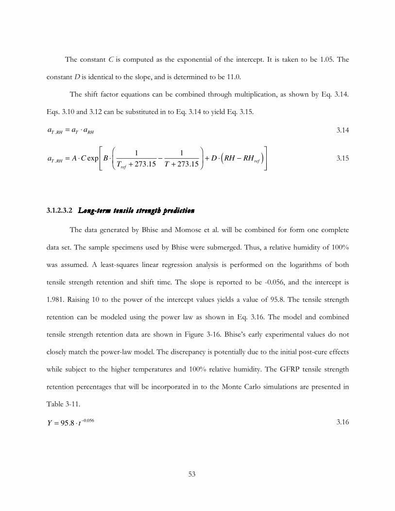
53
The constant C is computed as the exponential of the intercept. It is taken to be 1.05. The
constant D is identical to the slope, and is determined to be 11.0.
The shift factor equations can be combined through multiplication, as shown by Eq. 3.14.
Eqs. 3.10 and 3.12 can be substituted in to Eq. 3.14 to yield Eq. 3.15.
aT ,RH
= aT!a
RH 3.14
aT ,RH = A !C exp B !1
Tref + 273.15"
1
T + 273.15
#
$%
&
'( + D ! RH " RHref( )
)
*++
,
-..
3.15
3.1.2.3.2 Long-t erm t ens i le s t rength predi c t i on
The data generated by Bhise and Momose et al. will be combined for form one complete
data set. The sample specimens used by Bhise were submerged. Thus, a relative humidity of 100%
was assumed. A least-squares linear regression analysis is performed on the logarithms of both
tensile strength retention and shift time. The slope is reported to be -0.056, and the intercept is
1.981. Raising 10 to the power of the intercept values yields a value of 95.8. The tensile strength
retention can be modeled using the power law as shown in Eq. 3.16. The model and combined
tensile strength retention data are shown in Figure 3-16. Bhise’s early experimental values do not
closely match the power-law model. The discrepancy is potentially due to the initial post-cure effects
while subject to the higher temperatures and 100% relative humidity. The GFRP tensile strength
retention percentages that will be incorporated in to the Monte Carlo simulations are presented in
Table 3-11.
Y = 95.8 ! t"0.056 3.16

54
T
ensi
le s
tren
gth
rete
ntio
n [%
]
Shifted time [days]
Figure 3-16: Tensile strength retention versus shifted time for GFRP composites with
superimposed temperature and relative humidity effects. The power-law model for the
GFRP tensile strength retention is overlaid.

55
Table 3-11: Predicted long-term tensile strength retention for GFRP based on superimposed
relative humidity and temperature data.
Time Modeled tensile strength
retention
(years) (days) (%)
1 365 69
3 1095 65
10 3650 61
30 10950 57
60 21900 55
It should be noted that the glass fiber reinforced composite materials used by Bhise and
Momose et al. are not the same. The fiber volume fraction differed significantly between the two
sample types. The bars created by Hughes Brother contained a minimum of 70% glass fiber content
by weight [23]. The constant temperature of 71°C used in Momose et al. experiments is a higher
temperature than what any of Bhise’s bars were subject to in a water environment. The tensile
strengths between samples have been normalized by using tensile retention percentages to develop
the model, which negates the intrinsic sample material differences. Bhise’s samples were also subject
to an exposure time of 300 days of 100% relative humidity versus 120 days of variable humidity for
Momose et al. The combined model adequately reflects the combined effects of temperature and
moisture on the projected long-term tensile strength retention of GFRP bars.
3.2 Monte Carlo Simulations
The Monte Carlo technique was used to generate random variables. The concrete beam
geometry, concrete strength, as well as the GFRP bar tensile strength and modulus of elasticity was

56
randomized. Ten thousand random sample points were generated for each parameterized elements.
The sample points were used to determine the flexural capacity of a FRP reinforced concrete beam.
3.2.1 Random number g enera tion
The random numbers were generated using the built-in Random Number Generator in
Microsoft Excel. A uniform distribution of numbers between 0 and 1 is used. All randomly
generated numbers that are 0 and 1 are discarded, and new numbers are generated. The inverse of
the normal distribution is computed based on the mean and standard deviation of the parameterized
element as well as the probability of the event. The probability is equivalent to the randomly
generated number.
3.2.2 Parameter ized e l ements
The Monte Carlo simulation method relies on the application of probabilistic distribution
information to determine the parameters’ uncertainties. Beam geometry, concrete strength, and
tensile and modulus of elasticity of the GFRP bars are the critical parameterized elements in this
study. These variables can be used to determine flexural strength and failure strain criteria. The area
of the bars is not parameterized due to its deterministic nature.
3.2.2.1 GFRP tensile strength
The guaranteed tensile strength, as determined by manufacturers, can be used to determine
the bias, λ, and the coefficient of variation, V, for a set of GFRP bars. Bhise utilized #3 Hughes
Brothers bars [14]. Table 3-12 displays physical properties of the #3 bar as determined by Hughes
Brothers, which have been reproduced here with permission [23].

57
Table 3-12: Physical properties of #3 Aslan 100 GFRP Rebar by Hughes Brothers
Bar Size
Cross Sectional
Area* Nominal Dia.
Guaranteed
Tensile Strength
Tensile Modulus
of Elasticity
(mm) (inches) (mm2) (in2) (mm) (in) (MPa) (ksi) (GPa) psi 106
9 #3 84.32 0.1307 9.53 0.375 760 110 40.8 5.92
The bias of the tensile bar strength,
�
! f fu, can be determined via Eq. 3.17
! f fu=µ f fu
f fu 3.17
where
�
µ f fuis the mean experimental bar strength, and
�
f fu is the guaranteed tensile strength as based
on the retention percentages that were reported Table 3-12. The original tensile strength to be
applied to the retention percentages is approximately 85.6 ksi. The coefficient of variation, V, can be
computed using Eq. 3.18
Vffu=! f fu
µ f fu
3.18
where
�
! f fuis the standard deviation of the tensile strength.
A Weibull distribution can be fit to the experimental bar strength data [25]. The two main
parameters of the Weibull distribution are the shape parameter, m, and the scale parameter,
�
!o. The
parameters can be determined using either linear estimators or the process of maximum likelihood
estimation, MLE, both of which will be discussed in detail in Section 3.3.1.2 . Maximum likelihood
estimation will be used to determine all Weibull distribution parameters.
The Weibull parameters can be used to determine the mean bar strength and coefficient of
variation [25]. The mean bar strength is computed via Eq. 3.19

58
µ f fu= !
0"1+ m
m
#
$%&
'() !
0 3.19
where Γ the gamma function. The coefficient of variation, V, can then determined by Eq. 3.20.
Vffu=
!2 + m
m
"
#$%
&'
!2 1+ m
m
"
#$%
&'
(1 )1.2
m 3.20
A Weibull distribution has been fit to Bhise’s unconditioned plain bar specimens. The mean,
bias, and coefficient of variation have been determined. Okeil and Kulkarni conducted a similar
analysis on #2 through #10 FRP bars [25].
Table 3-13 provides a summary of the results for a #3 GFRP bar. There are differences
between the values reported by Bhise and Okeil and Kulkarni. These differences can be attributed to
dissimilar sample sizes and bar manufacturers.
Table 3-13: Statistical and mechanical properties of GFRP bars
Standard
Deviation COV
Weibull Distribution
Parameters Nominal
Tensile Strength Bias
�
! f fu
�
Vf fu
�
!o
Reference (MPa) (ksi)
�
! f fu (MPa) (ksi) (%) m (MPa) (ksi)
Bhise 590 85.6 0.778 11.14 1.615 2.07 61.8 595.3 86.3
Okeil and
Kulkarni
[25]
760 110 1.18 105.1 15.24 11.8 10.2 938.4 136.1
3.2.2.2 Concrete Strength
Concrete strength is used when determining the depth to the neutral axis. A quadratic
equation must be solved to obtain this parameter for the cases in which the GFRP bar does not

59
rupture. For this study, concrete strengths of 4000 (27,560), 5000 (34,450), and 6000 psi (41,340
kPa) will be considered.
Nowak and Szerszen conducted a statistical study to calibrate the steel reinforced concrete
design code. Strength of concrete, reinforcing steel bars, and pre-stressing strands were analyzed.
The bias and coefficient of variation values for ready-mix concrete under consideration are reported
in Table 3-14 [26].
Table 3-14: Statistical parameters of ordinary ready-mix concrete
�
! f c Mean
�
! f c
(kPa) (psi)
Number of
Samples (kPa) (psi) λ V
27,560 4000 116 34037 4937 1.235 0.145
34,450 5000 30 39,480 5726 1.15 0.058
41,340 6000 30 46,163 6695 1.12 0.042
3.2.2.3 Concrete beam and slab dimensions
Three dimensions are used to describe a concrete beam or slab. Figure 3-17 illustrates the
dimensions
Figure 3-17: Concrete beam with dimensions
b is the width of rectangular cross section; d is the distance from extreme compression fiber to the
neutral axis; and h is the overall height of the member. The dimensions are often reported in inches
or millimeters.

60
As part of their calibration study, Nowak and Szerszen also reviewed fabrication factors
when designing steel reinforced concrete structures. The fabrication factor refers to the natural
variations in dimensions and geometry during construction Fabrication factors for cast-in-place,
plant-cast, pre-stressed, and post-tensioned have been provided [26]. Only factors for cast-in-place
concrete were taken into consideration for this study.
Okeil et al. examined the reliability of bridge girders that had been strengthened by carbon
fiber-reinforced polymer laminates. Various statistical properties, namely the dimensions, were
reviewed prior to performing Monte Carlo simulations. Statistical property values were compared to
previously reported values [27]. Table 3-15 shows the results of the parameters provided by Nowak
and Szerszen as well as Okeil et al. The values for Okeil et al. will be used for the overall height of
the member, h.
Table 3-15: Statistical parameters of dimensional variables
Researcher Variable λ V
b 1.01 0.04 Nowak and Szerszen
[26] d 0.99 0.04
Okeil et al. [27] b,h,d 1.00 0.03
3.2.2.4 Summary of parameterized elements
Several variables were taken in account for the Monte Carlo simulations. Statistical
parameters of these variables have been obtained. Table 3-16 provides a summary of the variables as
well as the bias and coefficients of variation that will be incorporated into the simulations.

61
Table 3-16: Statistical properties of variables involved in this study
Researcher Variable λ V
b 1.01 0.04 Nowak and Szerszen
[26] d 0.99 0.04
Okeil et al. [27] h 1.00 0.03
4000 psi
(27,560 kPa) 1.235 0.145
5000 psi
(34,450 kPa) 1.15 0.058
Nowak and Szerszen
[26]
�
! f c
6000 psi
(41,340 kPa) 1.12 0.042
Bhise [14]
�
f f fu 0.78 0.0207
3.2.3 Flexural des ign of FRP re in fo rc ed concre te beams
The flexural strength of GFRP reinforced concrete beams was simulated using the Monte
Carlo technique. Each simulation consisted of the 10,000 data points.
3.2.3.1 Input values
The height and width of the concrete slab was input. Three geometric configurations werew
considered. The distance from extreme compression fiber to the centroid of tension reinforcement,
d, is computed by subtracting the clear cover distance from the overall height, h. A standard clear
cover value of 2.625 in. (66.675 mm) has been assumed for all of the configurations and is
completely arbitrary. Table 3-17 displays the dimensions and member name for each configuration.

62
Table 3-17: Member dimensions
b h d Member
Name (in) (mm) (in) (mm) (in) (mm)
A 12 304.8 24 609.6 21.375 542.925
B 9 228.6 16 406.4 13.375 339.725
C 18 457.2 48 1,219.2 45.375 1,152.5
The deterministic values presented in Table 3-17 were used as “mean values” to obtain
randomized dimensional elements. The standard deviation can be acquired by using the variance
information presented in Table 3-16 and Eq. 3.18.
Concrete compression strength values of 4000 (27,560), 5000 (34,450), and 6000 psi (41,340
kPa) will be considered. A similar procedure can be conducted to determine the “mean” and
standard deviation values for each of the concrete strengths.
Reinforced concrete design also utilizes a concrete calibration factor, β1, which was derived
by Whitney. β1 is 0.85 for concrete strengths of up to 4000 psi (28 MPa). A reduction of 0.05 is
taken for every 1,000 psi (7 MPa) increase in concrete strength. Eq. 3.21 will be used to
automatically calculate β1 for each of the concrete strengths. It should be noted that β1 can not be
less than 0.65 [15].
!1= 0.85 + 0.05 4 "
#fc1000
$%&
'()
3.21
3.2.3.2 GFRP reinforcement
The ACI 440 committee has established minimum levels of FRP reinforcement ratios. The
minimum ratios are of importance when designing reinforced structures with an expected failure
mode of FRP bar rupture. The minimum reinforcement area, Af, is similar in prescription to that of

63
steel reinforced concrete structures. Eq. 3.22 will be used to establish the minimum reinforcement
area.
Af ,min =4.9 !fc
f f fu
bwd "330
f f fu
bwd 3.22
where bw is the width of the web in inches. It should be noted that there is a separate equation for
metric units. All configurations under consideration have rectangular cross-sectional areas.
Therefore, the width of the web is taken to be the same as the width of the beam. Thus, Eq. 3.22
can be re-written as follows in Eq. 3.23.
Af ,min =4.9 !fc
f f fu
bd "330
f f fu
bd 3.23
The minimum reinforcement area does not apply to sections designed to fail via concrete
crushing, as the conditions of Eq. 3.22 are satisfied. The minimum reinforcement ratio, ρmin, can be
determined once Eq. 3.22 has been calculated via Eq. 3.24.
! f =Af
bd 3.24
Reinforcement ratios ranging from 0.1 to 1.4 times the balanced reinforcement ratio, ρfb,
were considered. The level of reinforcement is indicates whether over or under-reinforcement of the
FRP bars has been allocated by the designer. Under-reinforced sections are more susceptible to
failure via FRP bar rupture. Conversely, over-reinforced sections are designed to have concrete
crushing occur. It should be noted that a balanced reinforcement ratio is subject simultaneous FRP
bar rupture and concrete rushing. The balanced reinforcement ratio takes in to account the
mechanical properties for the FRP bars as well as the concrete strength. This ratio can be computed
by Eq. 3.25.

64
! fb = 0.85"1#fc
f f fu
E f$cu
E f$cu + f fu 3.25
where εcu is the ultimate strain in the concrete, and Ef is the design or guaranteed modulus of
elasticity of the FRP. The ultimate strain in concrete is always taken to be 0.003. The balanced area
of reinforcement is then back-calculated using both Eqs. 3.24 and 3.25.
The total number of reinforcement bars can be determined once the minimum balanced
reinforcement area is known. The reinforcement ratio associated with the total reinforcing bar area
is then computed. Fractions of the reinforcement ratio are then applied. The fraction of balanced
reinforcing ratio is increased by one-tenth for each round of simulations until 1.4 times the balanced
reinforcement ratio is achieved. The reduced reinforcement ratio and area are then determined. The
reduced values are compared to the minimums as established by Eqs. 3.23 and 3.24.
Using the power law model developed in Section 3.1.2.3 , the predicted age of the GFRP
bars can be applied to the model. The standard deviation is based on the unconditioned specimens,
which is 1615 psi (11 MPa). The unconditioned values for bar modulus of rupture and its standard
deviation are also used.
As per ACI 440 code, environmental reduction factors must be applied to the guaranteed
tensile strength of the FRP bars. The design tensile strength, ffu, is determined by Eq. 3.26 as follows
f fu = CE f fu* 3.26
where CE is the environmental reduction factor, and f fu* is the guaranteed tensile strength as defined
by Eq. 3.27. Environmental reduction factors of 0.7, 0.8, and 1.0 will be considered. The guaranteed
tensile strength is taken as the mean bar strength, fu,ave, minus three times the standard deviation [15].
f fu*= fu ,ave ! 3" 3.27

65
3.2.3.3 Strain-compatibility analysis
The flexural strength of under-reinforced FRP reinforced concrete members cannot be
calculated using the Whitney rectangular stress block. The maximum concrete strain of 0.003 may be
violated or not achieved, and is determined by the mode of failure. The depth to neutral axis, c, must
be determined. A quadratic equation for concrete design can be solved to determine the parameters
of c by using an approximation of the Whitney stress block. The three constants for the concrete
design quadratic are a1, b1, and c1. They can be calculated using Eqs. 3.28 - 3.30.
a1= 0.85 ! "
1!b ! #fc 3.28
b1= Af !Ef ! "cu 3.29
c1= Af !Ef ! "cu !d 3.30
Once the constants have been obtained, the quadratic formula may be applied determine the
depth to neutral axis. As shown below in Eq. 3.31, only the positive value of the quadratic is used.
c =b1+ b
1
2! 4 "a
1" c1
2 "a1
3.31
The FRP strain at rupture and at the ultimate condition of concrete strain may now be
ascertained. The ultimate strain, εcu, and FRP strain at rupture, εrupt, obtained via Eqs. 3.32 and 3.33,
respectively.
! fu =!cu
cd " c( ) 3.32
!rupt =f f
E f
3.33
A ratio of strains is also computed. A strain-based failure mode is selected. FRP bar rupture
is presumed to have occurred when the FRP strain rupture is greater than the ultimate strain.
Concrete crushing is the failure mode when ultimate strain is achieved before the bars have

66
ruptured. The strain-based failure mode then confirms the governing nominal flexural strength, as
will be discussed in Section 3.2.3.4 .
3.2.3.4 Nominal flexural strength
Although strain-compatibility analysis provides insight in to the failure mode, the flexural
strength of the FRP reinforced member is still unknown. Concrete crushing and FRP bar rupture
have separate processes to determine the appropriate flexural capacity.
The bar strength must be determined when designing for failure due to concrete crushing.
The bar strength is taken as the lesser of design tensile strength, ffu, and the tensile stress in the FRP
reinforcement, ff. The design tensile strength has been specified as an input value. The tensile stress
may be computed via. Eq. 3.34 [15].
f f =Ef ! "cu( )
2
4+0.85 ! #
1! $fc
% f
E f ! "cu & 0.5 !Ef ! "cu
'
(
))
*
+
,,- f fu 3.34
The flexural strength due to concrete crushing can be derived using Eqs. 3.35 and 3.36 [15].
Mn = Af f f d !a
2
"#$
%&'
3.35
where a is the depth equivalent of the rectangular stress block.
a =Af f f
0.85 ! "fc !b 3.36
The determination of a member’s flexural strength due to FRP bar rupture is more complex.
The quadratic equation for concrete stress-strain behavior must be solved to determine the flexural
capacity. The bar strength is based on the design tensile strength. Also, the depth to the neutral axis
is used instead the depth to the neutral axis as calculated by Eq. 3.31. Once obtained, the flexural
strength can be computed as follows in Eq. 3.37 [15].

67
Mn = Af f fu d !"1c
2
#$%
&'(
3.37
The flexural strength for each simulation is taken as the lesser of the flexural strength due to
concrete crushing or FRP bar rupture. The minimum values should coincide with the failure mode
predicted by the strain-compatibility analysis.
Information regarding the nominal slab design and Monte Carlo results are reported for each
simulation series. The nominal design moment is taken the flexural strength of the member based
on the deterministic input values. The design flexural strength is computed by applying a strength
reduction factor for flexure to nominal design value. The strength reduction factor is dependent
upon the balanced and calculated values for the reinforcement ratio. Eq. 3.38 provides the guidelines
for selecting the correct strength reduction factor.
! =
0.55 for " f # " fb
0.3+ 0.25" f
" fb
for " fb
0.65 for " f $ 1.4" fb
%
&
''
(
''
< " f < 1.4" fb 3.38
The average flexural strength for the Monte Carlo simulations is computed. The standard
deviation and coefficient of variation are also reported for each set. All flexural strengths are
obtained in both English and SI units. The number of simulations below the nominal and design
flexural strengths are tabulated. The number of rupture failures is also counted.
3.3 Reliability assessment
The reliability assessment relies on determining an appropriate cumulative density function to
model the flexural strength data. The Monte Carlo simulations are based on normally distributed
random variables. The Weibull distribution will be used to model the flexural strength. The specific
parameters of the distribution must be obtained for each simulation. Confidence intervals will be

68
determined for both the Weibull parameters as well as the reliability function for the flexural
strength.
3.3.1 Weibul l dis tr ibut ion mode l s
Scientists and engineers often use the Weibull distribution. The distribution is readily
applicable to many different types of data sets. The distribution is flexible, and its parameters are
easily obtained through a variety of numerical methods.
Extreme value theory can be used to identify the third asymptotic distribution. Fisher and
Tippet originally derived this distribution. Waloddi Weibull used the distribution to review breaking
strengths, and now bears it namesake [28]. The Weibull distribution will be used to model the
flexural strength for each configuration.
3.3.1.1 Background on the Weibull distribution
A Weibull model can be based on either two or three parameters. The three parameters are
shape, scale, and location. The notation describing the distribution varies. For this study, Dodson’s
notation will be used. The Weibull probability density function is described below in Eq. 3.39
f x( ) =! x " #( )
!"1
$! exp "x " #$
%&'
()*!+
,--
.
/00, x 1 # 3.39
where β is the shape parameters, θ is the scale parameter, and δ is the location parameter [29]. The
shape parameter may be also referred to as the Weibull modulus.
The Weibull cumulative density function is described by Eq. 3.40 as
FXx( ) = 1! exp !
x ! "#
$%&
'()*+
,--
.
/00
3.40

69
The Weibull reliability function will be used more often than the Weibull cumulative density
function. The function is often computed as the one minus the cumulative density function. A more
formal definition of the Weibull reliability function is shown below in Eq. 3.41.
R x( ) = exp !x ! "#
$%&
'()*+
,--
.
/00
3.41
The shape parameter, β, alters the shape of the probability density function, as seen in Figure
3-18 [29]. The shape parameter is characteristic property of the modeled data set. For example, the 0
and 60 year Monte Carlo simulation configurations will have the same shape parameter but different
scale parameters.
Figure 3-18: The Weibull probability density function [29]
Murthy et al. have proposed that there are seven different Weibull models. Table 3-18 shows
the types and descriptions of Weibull models [30].

70
Table 3-18: Taxonomy for Weibull Models.
Type Description
I Transformation of Weibull Variable
II Transformation of Weibull Distribution
III Univariate Models involving Multiple Distributions
IV Varying Parameters
V Discrete Models
VI Multivariate Models
VII Stochastic Models
A goodness-of-fit test such as Chi-square or Kolmogorov-Smirnov can be used to determine
the appropriate type of model. The standard Weibull distribution will be used in this study, which is
a Type II model. Although the two-parameter distribution results in lower nominal strengths, there
is only a 1% decrease in values [31]. The location parameter has been assumed to be equal to zero.
Therefore, a two-parameter Weibull distribution will be used.
3.3.1.2 Methods for estimating parameters
Graphical and statistical methods may be used to determine the parameters of the Weibull
distribution. The statistical methods include moment estimator, percentile estimator, maximum-
likelihood estimator, Bayesian estimator, and interval estimator. The graphical method often relies
on plotting the data and fitting it to a line [30]. The linear and maximum likelihood estimators are
the only methods of interest in this study.
The easiest way to obtain the Weibull parameters is by using linear estimators. The slope of
the line is the Weibull modulus. The scale parameter can be taken as the exponential of the negative
ratio of between slope and intercept. The linear estimators provide a good estimate. However, the
method of maximum likelihood provides the most accurate results for the Weibull parameters [29].

71
The method of maximum likelihood provides a more robust estimate for the Weibull
parameters. The parameters may be obtained by simultaneously solving Eqs. 3.42 - 3.44 [31]. The
Solver feature of Microsoft Excel was used to solve the simultaneous equations.
xi! "( )
#ln x
i! "( )
i=1
n
$
xi! "( )
i=1
n
$!1
#%&'
()*!
ln xi! "( )ni=1
n
$ = 0
3.42
! =
xi" #( )
$
i=1
n
%n
&
'
((((
)
*
++++
1
$
3.43
!
"!xi# $( )
i=1
n
%!#1
# ! #1( ) xi# $( )
i=1
n
%#1
= 0 3.44
3.3.1.3 Development of confidence intervals
Given the large sampling size for each simulation, nearly exact confidence intervals may be
obtained. All data points will be considered uncensored. Ninety-fifth percentile confidence intervals
for the parameters and overall distributions can be determined after the Weibull scale and shape
parameters are known. Dodson outlines the process for ascertaining both sets of confidence
intervals [29]. The confidence intervals for the parameters will be determined prior to the
distribution’s intervals.

72
3.3.1.3.1 Confidence int ervals for Weibu l l parameters
Confidence intervals were obtained for the scale and shape parameters. The location
parameter has been assumed to be equal to 0. Thus, no confidence intervals can be determined. The
flexural strength simulation points must be sorted in to an ascending order [29].
First, the confidence intervals for the shape parameter were calculated. The second
derivative of the of the log-likelihood function with respect to the scale parameter is determined for
each uncensored data point using Eq. 3.45.
!2Lu
!" 2=
#" 2
$xi
"%&'
()*# #
" 2%&'
()*# +1( ) 3.45
Next, The second derivative of the of the log-likelihood function with respect to the shape
parameter is determined for each uncensored data point using Eq. 3.46.
!2Lu
!" 2= #
1
" 2#
xi
$%&'
()*"
lnxi
$%&'
()*
+
,-
.
/0
2
3.46
Third, the second derivate of the log-likelihood function with respect to both the scale and
shape parameters is calculated for each uncensored data point using Eq. 3.47.
!2Lu
!"!#= $
1
#+
xi
#%&'
()*"1
#" ln
xi
#%&'
()*+1
+
,-
.
/0 3.47
A similar process is conducted for each of the censored points. The second derivatives for
the censored points are equal to zero, as there are no censored points. The equations have been
included for future reference though. The second derivative of the log-likelihood function with
respect to the scale parameter is obtained via Eq. 3.48.
!2Lc
!" 2= #
xi
"$%&
'()* *
" 2$%&
'()* +1( ) 3.48

73
The second derivative of the log-likelihood function with respect to the shape parameter is
determined via Eq. 3.49.
!2Lc
!" 2= #
xi
$%&'
()*"
lnxi
$%&'
()*
+
,-
.
/0
2
3.49
The second derivate of the log-likelihood function with respect to both the scale and shape
parameters is calculated for each censored data point using Eq.
!2Lc
!"!#=
xi
#$%&
'()"1
#$%&
'()
" lnxi
#$%&
'()+1
*
+,
-
./ 3.50
The second derivatives for both the uncensored and censored data points with can be used
to determine the local information matrix. This matrix will be used when obtaining confidence
intervals for both the scale and shape parameters. The local information matrix is obtained using Eq.
3.51.
F =
!"L
T
2
"# 2!
"LT
2
"$"#
!"L
T
2
"$"#!"L
T
2
"$ 2
%
&
''''
(
)
****
3.51
where
!2LT
!"2=
!2Lui
!"2
i=1
r
# +!2Lci
!"2
i= r+1
n
# 3.52
!2Lt
!" 2=
!2Lui
!" 2+
!2Lci
!" 2
i= r+1
n
#i=1
r
# 3.53
!2LT
!"!#=
!2Lui
!"!#+
!2Lci
!"!#i= r+1
n
$i=1
r
$ 3.54
Additionally, r is the number of failures, while n is the total number of data points. Both are equal to
10,000 for the data sets used because the system is assumed to have failed. Furthermore, the number

74
of failures is the identical to the number of uncensored data points. It should be noted that all
summations involving censored points are equal to zero.
The local information matrix is then inverted. The parameters are often referred to the
following as noted in Eq. 3.55. The variance of the scale parameter is equal to F(1,1)
!1 . The variance of
the shape parameter is equal to F(2,2)
!1 . The covariance of the scale and shape parameters is equal to
F(1,2)
!1 .
F!1=
F(1,1)
!1F(1,2)
!1
F(2,1)
!1F(2,2)
!1
"
#$%
&' 3.55
Ninety-five percent confidence limit states were used. The lower and upper confidence limits
for the shape parameter are determined by Eqs. 3.56 and 3.57, respectively.
!L=
!
expK F(2,2)
"1
!
#
$%%
&
'((
3.56
!U= ! exp
K F(2,2)"1
!
#
$%%
&
'((
3.57
where K is the standard normal percentile for the percent limit as determined by Eq. 3.58.
K = 100 1!"2
#$%
&'(
3.58
The percent limit is based on Eq. 3.59
100 1!"( ) 3.59
and α is the percentile of interest. The 95th percentile has an α value of 0.05 and is equal to a 97.5th
standard normal percentile. Therefore, K can be computed as the inverse of the standard normal
distribution, and is approximately equal to 1.96.

75
The lower and upper confidence limits for scale parameter can be readily calculated via Eqs.
3.60 and 3.61, respectively.
!L=
!
expK F(1,1)
"1
!
#
$%%
&
'((
3.60
!U= ! exp
K F(1,1)"1
!
#
$%%
&
'((
3.61
3.3.1.3.2 Confidence int ervals for Weibu l l di s t r ibut ions
Confidence intervals for Weibull distributions examine the reliability of the data set. The
method of maximum likelihood will be used to determine the 95th percentile confidence intervals.
In recalling Eq. 3.55, variances of the estimates are automatically calculated. The variance of the
scale parameter is equal to F(1,1)
!1 . The variance of the shape parameter is equal to F(2,2)
!1 . The
covariance of the scale and shape parameters is equal to F(1,2)
!1 .
RLx( ) = e
! exp u+K var u( )( ) 3.62
RUx( ) = e
! exp u!K var u( )( ) 3.63
where
u = ! ln x( ) " ln #( )$% &' 3.64
var u( ) = ! 2 var "( )
" 2#$%
&'(+
u2var !( )
! 4
#$%
&'()2u cov !,"( )
! 2"#$%
&'(
*
+,
-
./ 3.65
Eq. 3.65 can be re-written in terms of the inverted local information matrix values, and is
shown in Eq. 3.66.

76
var u( ) = ! 2F(2,2)
"1
# 2$
%&'
()+
u2 *F
(1,1)
"1
! 4
$
%&'
()"2u *F
(1,2)
"1
! 2#
$
%&'
()+
,--
.
/00
3.66
3.3.2 Determinat ion of env ironmental re duc tion fac tors
The American Concrete Institute requires the application of an environmental reduction
factor to the guaranteed tensile strength of FRP. Values are based on the exposure conditions that
the concrete is subject to, and were shown in Table 2-3. The goal is to determine a reduction factor
such that the initial FRP tensile strength is reduced by a sufficient amount, and thereby
approximates the projected long-term tensile strength of the material. A reliability-based approach
was used to determine appropriate environmental reduction factors.
3.3.2.1 Monte Carlo simulations for bar strength
This portion of the study seeks to determine more appropriate factors. According to Eq.
3.26, the design tensile strength is directly related to the environmental reduction factor. Therefore,
it is the only randomized variable for these Monte Carlo simulations. Age-defined tensile strength
values were based on the Power Law model described in Sec. 3.1.2.3 , and were used as the mean
bar strength. The standard deviation is based on the unconditioned GFRP bar data provided by
Bhise.
The concrete members were presumed to be subject to flexure. They were designed in
accordance with the procedure outlined in Sec. 3.2.3 . Ten thousand simulations for GFRP tensile
strength were performed for 0, 1, 3, 10, 30, and 60 years. Unique values for the environmental
reduction will be determined for each of the years.

77
3.3.2.2 Computational procedure
The development of the design tensile strength of FRP takes in to account the mean minus
three standard deviations value, which is the guaranteed tensile strength. For a normal distribution,
the 3 standard deviations pertain to 6 standard deviations over the data range. Therefore, 99.73% of
the data will lie under the area of the normal distribution curve. The lower tail of -3σ represents the
bottom 0.135% of the normal cumulative distribution function (CDF). Conversely, the upper tail of
+3σ refers to 99.865% of the normal CDF.
The Weibull distribution is generally not symmetric like the normal distribution. The upper
and lower tails can be obtained manually or via approximation. The approximation of tails selects
data values at 99.9% and 0.01%, which is very similar to having 99.73% of the data lying under the
normal CDF. The alternative approach is to obtain the mean and standard deviation of the Weibull-
modeled data. The mean plus or minus three standard deviations can be determined. The manual
method of determining the tails were used. Once the lower tail of the Weibull distribution has been
determined, its corresponding reliability value may be obtained via Eq. 3.41.
Okeil and Kulkarni have shown that FRP bar strength can be modeled using a Weibull
distribution [25]. The Weibull distribution for the bar strength can be transformed in tot a
distribution for flexural strength. Ninety-five percent upper and lower reliability limits will be
determined based the flexural strength. The mean, standard deviation, and coefficient of variation
will be computed.
The tail analysis was performed on the initial data to determine the corresponding reliability
level. In the following derivation, the initial conditions and time dependent conditions are denoted
as t1 and t2, respectively. The upper reliability tail of minus three standard deviations is computed by
Eq. 3.67.

78
Mn( )
t1
= µt1! 3"
t1 3.67
The flexural strength can then be substituted in to Eq. 3.41. The re-written equation is
shown below in Eq. 3.68.
R = exp !M
n( )t1
"t1
#
$%
&
'(
)*
+
,,
-
.
//= exp !
µt1! 30
t1
"t1
#
$%
&
'(
)*
+
,,
-
.
//
3.68
The reliability will be applied to obtain the age specific flexural strength. The flexural
strength can be written in terms of either the reliability and Weibull distribution parameters or the
deterministic flexural strength equation. Both options are displayed in Eq. 3.69.
Mn( )t2= !t2 ln
1
R
"#$
%&'
1
()
*
++
,
-
.
.= Af CE fu ,ave / 30( ))* ,- d /
(1c
2
)*+
,-.
123
456t2
3.69
The environmental reduction factor can be see as the fraction of strength retained under
harsh exposure conditions. Thus, the environmental reduction factor can be approximated as the
ratio of the reliability-based aged tensile strength and the unconditioned guaranteed tensile strength.
The overall mathematical expression for the environmental reduction factor is presented in Eq. 3.70.
CE =
!t2 ln1
R
"#$
%&'
1
()
*
++
,
-
.
.
Af d /(1c
2
)*+
,-.
0
1
222
3
222
4
5
222
6
222t2
fu ,ave / 37( ){ }t1
3.70
The process was repeated for each of the simulation years. Concrete strength and beam
geometry will also be varied. The environmental reduction factor at both time intervals and the 60-
year mark will also be incorporated in to the Monte Carlo simulations. Comparisons between the
recommended environmental reduction factor and those mandated by the ACI code will be made.

79
3.3.3 Determinat ion of s t reng th reduc ti on fac t or s
The current ACI values for the strength reduction factor are based on the desired failure
mode and level of reinforcement. Factors can be selected using Eq. 3.38. The basis for the values is
derived from the ACI code for steel reinforced concrete structures. There is a need to determine
strength reduction values based on the behavior FRP material itself.
Three different approaches were used to determine strength reduction factors. The
corresponding design flexural strength will be resolved for each Monte Carlo simulation using Eq.
3.71
Mn Design( )= ! Mn Nomin al( )( ) 3.71
where φ is the strength reduction factor; and MnNomin al( )
is the nominal flexural strength. The nominal
flexural strength is taken as the minimum flexural strength value per the limit state flexural strength
function for either concrete crushing or FRP bar rupture.
The first factor was selected in accordance with Eq. 3.38. Based on the fractions of
reinforcement ratios under consideration, most design values will incorporate a strength reduction
factor of 0.55.
Ellingwood has outlined the critical need to apply a load and factor resistance (LFRD)
approach in determining the strength reduction factors. LFRD has been successfully applied to
wood and steel structure design. Composite materials, such as FRP, can also be designed using
LFRD. An approximate value of a resistance factor can be obtained using Eq. 3.72
! =µR
Rn
"
#$%
&'exp ()
R* + *V
R[ ] 3.72
where µR is the mean resistance level; Rn is the nominal strength; αR is the sensitivity coefficient; β is
the safety index; and VR is the variability.

80
The mean resistance level is the average flexural strength of all simulations. The variability
will be taken as the coefficient of variation of the flexural strength. The sensitivity coefficient has
been assumed to be 0.6 [19]. ACI has a minimum factor of safety, β, of 3.5, with an allowable range
of 3.5 – 4 [15]. For the purposes of this study, safety factors of 3.5 and 4 are considered using Eq.
3.72. Numerical substitutions can be made, and Eq. 3.72 can then be re-written as Eqs. 3.73 and
3.74 for the minimum and maximum safety factors, respectively. Ellingwood’s approach will
constitute the second strength reduction factor.
! =µM
n
Mn Nominal( )
"
#$$
%
&''exp (2.1 )V
R[ ] 3.73
! =µM
n
Mn Nominal( )
"
#$$
%
&''exp (2.4 )V
R[ ] 3.74
The third strength reduction factor was obtained using the brute force method. A maximum
value for Eq. 3.71 was obtained by solving for a strength reduction factor. An additional constraint
is imposed on Microsoft Excel Solver. The design value is considered by design practice as the
minimum flexural strength value. Therefore, the strength reduction factor must be achieved such
that the number of simulations falling below the design value is identically zero.
The ACI strength reduction factors serve as the control factors. Comparisons between ACI
and the second and third approaches are made. The number of simulations falling below the revised
design flexural strength is tabulated.

81
CHAPTER 4 Results
4.1 Introduction
Monte Carlo simulations were performed to model the flexural strength and durability of
GFRP reinforced concrete beams. Simulations were based on varying the parameters involved in
calculating the flexural capacity. The modeled long-term tensile strength of GFRP bars was used to
assess fitting environmental reduction factors. Flexural strength reduction factors were computed
and compared.
4.2 Environmental Reduction Factors
Prior to beginning the full-scale Monte Carlo simulation procedure, appropriate
environmental reduction factors were ascertained. Environmental reduction factors were expected
to act as “knock down” factors when applied to initial GFRP bar tensile strengths. The reduction
was expected to be significant enough to such that the newly computed bar tensile strength values
and the projected long-term tensile strength values would be in close proximity to each other. The
mean minus three standard deviations for flexural strength of a GFRP reinforced concrete member
corresponds to a reliability of approximately 0.9890 for all simulations. Figure 4-1 is a representative
illustration, which highlights the initial difference in Weibull-based moment capacities when the
projected 0 and 60 year GFRP tensile strength values are applied.

82
Rel
iabi
lity
Flexural strength [k-in]
Figure 4-1: Comparison of Weibull-based moment capacities for Member A using projected
0 and 60 year GFRP tensile strength values
Eq. 3.70 was used to calculate the environmental reduction factor to convert the initial
strength distribution. A factor of 0.5 was obtained. Figure 4-2, which is a representative illustration,
displays Weibull-based flexural strengths for Member A based on initial, revised, 60-year, and ACI
based GFRP tensile strengths. The revised strength was determined by applying the calculated
environmental reduction factor of 0.5 to the initial GFRP tensile strength. The ACI based
distribution utilizes an environmental reduction factor of 0.7, which is in accordance with current
design code provisions.
All four of the Weibull-based flexural strength distributions have been included on the figure
for comparative purposes. The ACI-based flexural strength distribution does not closely match the

83
projected strength values at 60 years, and provides an overestimate of the strength retention. The
application of the ACI exposure factor could potentially lead to unsatisfactory flexural strength for
the reinforced member over the anticipated service life.
Rel
iabi
lity
Flexural strength [k-in]
Figure 4-2: Comparison of Weibull-based moment capacities for Member A using both 0
year and 60-year projected GFRP tensile strength values. The 0 year revised and ACI
moment capacities have incorporated environmental reduction factors of 0.5 and 0.7,
respectively, to the 0-year GFRP tensile strength.
All of the time-dependent environmental reduction factors were collected and compared to
the ACI values. A representative plot is shown in Figure 4-3. The currently prescribed ACI values
are shown as constant horizontal lines over the service life of the structure. The environmental
reduction factors shown were obtained for all three members at the specific service age level.

84
Concrete strength and beam geometry were determined to have no bearing on the environmental
reduction factor using the outlined approach. Given a life-cycle of 60 years of exposure, a more
appropriate environmental reduction factor would be 0.5. This factor is also taken in to
consideration for the remaining Monte Carlo simulations. The trend of decreasing environmental
reduction factors with time is expected due to the loss of GFRP strength over time.
Aside from the ACI prescribed values, the environmental reduction factors presented in
Figure 4-3 represent GFRP reinforced concrete members that are exposed to earth and weather. It
has been assumed that these reinforced concrete members are subject to nearly 100% relative
humidity. However, it is possible that alternative environmental reduction values exist for situations
in which the FRP reinforced concrete members are designed for other relative humidity conditions.
Such instances would indicate an indoor exposure level, which could produce an environmental
value similar to what ACI currently proposes. This study has not accounted for these instances, and
entirely deals with GFRP reinforced concrete members that are exposed to earth and weather.

85
Env
iron
men
tal r
educ
tion
fact
or [
CE]
Time [years]
Figure 4-3: Environmental reduction factors for Member A designed with 4000 psi concrete
as a function of time.
4.3 Monte Carlo simulation results
Many Monte Carlo simulations were performed during this study. The environmental
reduction factors proposed in Sec. 4.2 were utilized to determine the appropriate projected long-
term GFRP bar tensile strength. The effects of beam geometry, concrete strength, and fractions of
the balanced reinforcement ratio will be considered. Nominal flexural strength, percentage of
simulation failures due to GFRP bar rupture, percentage of simulations with a flexural strength
below the nominal value are used to draw comparisons and contrasts between each of the effects
under consideration.

86
4.3.1.1 Effect of environmental reduction factors
The environmental reduction factors, which were established in Sec. 4.2 , were used in the
Monte Carlo simulations. The factors were used in Eq. 3.26 to determine the design tensile strength.
The flexural strength was then computed for either concrete crushing or FRP bar rupture. Figure
4-4 shows the Weibull mean for nominal flexural strength for Member A with 4000 psi. The error
bars shown are based on the Weibull standard deviation for the modeled flexural strength.
The balanced reinforcement condition is shown. The flexural strength increases with
increasing environmental reduction factors. The trend, as demonstrated by the representative
illustration, is expected due to the direct relationship between the environmental reduction factor
and design tensile strength. The ACI values of 0.7 and 0.8, for exposed and unexposed concrete,
produced greater flexural strength values than those calculated in Sec. 4.2 . The ACI prescribed
environmental reduction values inflate the retained tensile strength, and thus, produces higher than
achievable long-term nominal flexural strength.

87
Wei
bull-
base
d no
min
al fl
exur
al s
tren
gth
[k-i
n]
Environmental reduction factor [CE]
Figure 4-4: Weibull-based nominal flexural strength as a function of environmental
reduction factor for Member A designed with 4000 psi concrete at balanced reinforcement
ratio conditions.
Figure 4-5 shows the percentage of simulations occurring below the nominal flexural
strength as a function of environmental reduction factor. The percentages range from 25 – 50% for
all simulations conducted. The lowest percentage for all simulations occurred for the configurations
designed with a concrete strength 6000 psi and a reinforcement ratio fraction of 1.2.
In general, lower environmental reduction factors lead to greater susceptibility to fail via
FRP bar rupture. The trend can be tied to the underestimation of long-term strength via the
application of the environmental reduction factor. As corroborated by Figure 4-4, lower
environmental reduction factors lead to lower nominal flexural strengths for the GFRP reinforced
concrete members. When an environmental reduction factor is not considered, as is the case when it

88
is equal to 1, the number of simulations falling below the nominal flexural strength slightly increases.
The balanced condition indicates the potential to have simultaneous concrete crushing and FRP bar
rupture. Therefore, the increase may be attributed to the randomness of the simulations, and the
propensity to fail via FRP bar rupture. The result for the configuration is in relative proximity to the
other values.
Per
cent
age
of s
imul
atio
ns b
elow
nom
inal
flex
ural
str
engt
h [%
]
Environmental reduction factor [CE]
Figure 4-5: Percentage of simulations occurring below the nominal flexural strength for
GFRP reinforced concrete members as a function of the environmental reduction factor for
Member A designed with 4000 psi concrete and balanced reinforcement ratio conditions.
The only two failure modes under consideration are FRP bar rupture and concrete crushing.
The third area of analysis pertains to the number of simulations that failed due to FRP bar rupture.
In a mathematical sense, one of the failure modes will always precede the other mode. However,

89
physically, there are many instances, especially around the region of balanced reinforcement ratio, in
which both failure modes due successfully occur simultaneously. Figure 4-6 is shown as a
representative illustration. The projected environmental reduction values produced yielded all
simulations failing due to FRP rupture. The design tensile strength is nearly halved by the
application of the most of the computed factors. It is expected that the reduction would adversely
impact the strength of the member and lead to more bar ruptures. The lowest percentages achieved
in this area were for the simulations in which the environmental reduction factor was not included.
If failure due to FRP bar rupture is desired, the proposed factors succeed in guaranteeing the
preferred failure mode.
Per
cent
age
of F
RP
bar
rup
ture
failu
res
[%]
Environmental reduction factor [CE]
Figure 4-6: Percentage of failures out of 10,00 simulations due to FRP bar rupture for
Member A designed with 4000 psi concrete and balanced reinforcement ratio conditions.

90
4.3.1.2 Effect of beam geometry
Three different member sizes were considered for the simulations. Members A and C are
analyzed for comparative purposes. The reinforcing area and fractions of reinforcement ratio will be
compared.
Figure 4-7 and Figure 4-8 show the reinforcing bar area as a function of the fraction of
balanced reinforcement ratio for Members A and C, respectively. The initial constant values for
reinforcing area is due to the minimum area requirements imposed by Eq. 3.23. The minimum area
is invoked for fractions of reinforcement ratio ranging from 0.1 – 0.7. The total reinforcing bar area
is dependent upon the member width, b, and the distance from extreme compression fiber to the
centroid of tension reinforcement, d. It is expected that the larger geometry of Member C will
require more FRP bars for reinforcing. As shown by the figures, the effect of geometry on the area
is minimized by an increase of the concrete strength. The required reinforcing linearly increases with
fractions of reinforcement ratio for all other values.

91
GF
RP
rei
nfor
cing
bar
are
a [i
n2 ]
Fraction of balanced reinforcement ratio
Figure 4-7: Total GFRP reinforcing bar area for Member A with respect to varying concrete
strength and fractions of balanced reinforcement ratio.

92
GF
RP
rei
nfor
cing
bar
are
a [i
n2 ]
Fraction of balanced reinforcement ratio
Figure 4-8: Total GFRP reinforcing bar area for Member C with respect to varying concrete
strength and fraction of balanced reinforcement ratio.
Figure 4-9 compares the nominal flexural strength as a function of reinforcing ratio for
members A and C. The balanced conditions with a concrete strength of 4000 psi were used the
illustration shown. There is a kink in the data for both of the members. The kink coincides with the
transition from relying on the minimum reinforcing to utilizing reinforcing areas based on the
applied fraction of the balanced reinforcement ratio. There is a tremendous gap in the nominal
strength achieved by the two members. The gap can be attributed to the significantly larger moment
arm produced by the dimensions of Member C. Namely, the depth of Member C is twice as large as
the depth of Member A.

93
Nom
inal
flex
ural
str
engt
h [k
-in]
Total GFRP reinforcing area [in2]
Figure 4-9: Nominal flexural strength for GFRP reinforced concrete members with respect
to total GFRP reinforcing bar area for Members A and C. The illustrations shown are used
to draw contrast to different beam geometries of the different members.
The flexural strength of a FRP reinforced member is both directly and indirectly dependent
upon the beam geometry. As seen by Eqs. 3.35 and 3.36, for concrete crushing failure, flexural
strength will increase with larger distances from extreme compression fiber to the centroid of
tension reinforcement. Larger d values can be compensated by utilizing a larger beam width. The
beam geometry is also an integral component of in determining the constants of the concrete design
quadratic. It is expected that larger d and b values will produce bigger flexural strength values.
Figure 4-10 and Figure 4-11 show the nominal flexural strength for Members A and C as a
function of the fraction of balanced reinforcement ratio. All environmental reduction factors under

94
consideration have been plotted. The initial constant values for the flexural strength are present due
to the aforementioned consequence of the minimum FRP reinforcement. The flexural strength for
member A ranges from approximately 800 – 3000 k-in. Conversely, the flexural strength range for
Member C ranges from 5000 – 19000 k-in. The maximum value achieved by Member A is barely
60% of the minimum value for Member C.
Nom
inal
flex
ural
str
engt
h [k
-in]
Fraction of balanced reinforcement ratio
Figure 4-10: Nominal flexural strength for GFRP reinforced concrete Member A with
respect to environmental reduction factor and fraction of balanced reinforcement ratio. The
member was designed with 4000 psi concrete.

95
Nom
inal
flex
ural
str
engt
h [k
-in]
Fraction of balanced reinforcement ratio
Figure 4-11: Nominal flexural strength for GFRP reinforced concrete member C with respect
to environmental reduction factor and fraction of balanced reinforcement ratio. The member
was designed with 4000 psi concrete.
Figure 4-12 and Figure 4-13 display the percentage of failures due to FRP bar rupture for
both members A and C. For the information shown, the members were designed with 4000 psi. All
fractions of reinforcement ratio as well as environmental reduction factors are demonstrated. One
hundred percent of all simulations for both cases up to 0.8 of the reinforcement ratio were
determined to fail due to FRP bar rupture. The declines in the percentages have been attributed to
the environmental factors, and not the increase in geometry. Therefore, and although Member C is
significantly larger than Member A, it is equally prone to the FRP bar rupture failure mechanism.

96
Per
cent
age
of s
imul
atio
n fa
ilure
s du
e to
FR
P b
ar r
uptu
re [
%]
Fraction of balanced reinforcement ratio
Figure 4-12: Percentage of simulation failures due to FRP bar rupture for Member A
designed with 4000 psi concrete with respect to fractions of balanced reinforcement ration
and environmental reduction factor. All environmental reduction factors were subject to
100% FRP bar rupture failure except for factors of 0.8 and 1.0.

97
Per
cent
age
of s
imul
atio
n fa
ilure
s du
e to
FR
P b
ar r
uptu
re [
%]
Fraction of balanced reinforcement ratio
Figure 4-13: Percentage of simulation failures due to FRP bar rupture for Member C design
with 4000 psi concrete and with respect to fractions of balanced reinforcement ration and
environmental reduction factor. All environmental reduction factors were subject to 100%
FRP bar rupture failure except for the factors of 0.8 and 1.0.
4.3.1.3 Effect of concrete strength
The minimum reinforcing area is dependent on the beam geometry and concrete strength, as
per Eq. 3.23. The effects of concrete strength on the nominal flexural strength and the percentage of
failures due to FRP bar rupture will be examined in this section. For illustrative purposes, the figures
shown have been based on data from Member A with no environmental reduction factor applied.
Figure 4-14 displays the nominal flexural strength versus the fraction of balanced
reinforcement ratio. The results for 4000, 5000, and 6000 psi concrete are shown. The initial
expectation was that higher concrete strengths would produce larger nominal flexural strength

98
values. The trend is exemplified by the figure. Greater concrete strengths lead to the minimum
reinforcement being considered over a smaller range due to its indirect relationship. It has been
corroborated Figure 4-10 and Figure 4-10. The concrete strength also impacts the β1 value, which is
based on the concrete strength and is an important factor in reinforced concrete designed for
flexure.
Nom
inal
flex
ural
str
engt
h [k
-in]
Fraction of balanced reinforcement ratio
Figure 4-14: Nominal flexural strength for GFRP reinforced concrete Member A with
respect to fractions of balanced reinforcement ratio and concrete strength.
Figure 4-15 compares the percentage of failures attributed to FRP bar rupture for the three
concrete strengths. All three concrete strengths behaved similarly for fractions of reinforcement
ratio up to approximately 0.8. Over this range, all simulations failed due to FRP bar rupture. The

99
results are consistent with effects on rupture from beam geometry and reinforcement area.
However, 4000 psi concrete produced fewer FRP bar rupture simulation failures at a lower fraction
of balanced reinforcement ratio. For the over-reinforced sections, which should be more prone to
concrete crushing by definition, the 5000 and 6000 psi behaved identically and ultimately failed to
reduce the vulnerability to FRP bar rupture failure.
Per
cent
age
of s
imul
atio
n fa
ilure
s du
e to
FR
P b
ar r
uptu
re [
%]
Fraction of balanced reinforcement ratio
Figure 4-15: Percentage of simulation failures due to bar rupture with respect to fraction of
balanced reinforcement ratio for Member A designed with 4000, 5000, and 6000 psi concrete.
Values of 100% indicate all 10,000 simulations experienced this failure mode.

100
4.4 Strength reduction factors
Four methods were used to determine flexural strength reduction factors. The first method
is based current ACI code provisions. The second and third methods are based on an LRFD derived
equation by Ellingwood for two different factors of safety. The final method is based on using brute
force calculations. The figures shown are representative of the trends demonstrated by the three
concrete members for all three concrete strengths. For illustrative purposes, the results of member A
with a concrete strength of 4000 psi are displayed.
The ACI flexural strength reduction factors were determined for each simulation using Eq.
3.38. Figure 4-16 displays the relationship between fractions of the reinforcing ratio and the ACI
strength reduction values. The strength reduction factor has a constant value for fractions of the
balanced reinforcement ratio less than one. For other fractions of the balanced reinforcement ratio,
the flexural strength reduction increases as expected, which is in accordance with the ACI guidelines.
Figure 4-16 also extends the fraction of balanced reinforcement ratio beyond what has been
considered for the Monte Carlo simulations. The extension was used to verify the constant strength
reduction factor of 0.65 for reinforcement conditions greater than 1.4 times the balanced
reinforcement ratio. The FRP bar rupture governed simulations are subject to more strength
reduction than members who fail via concrete crushing. There were no simulations achieving a
flexural strength less than the ACI-based design value.

101
Fle
xura
l str
engt
h re
duct
ion
fact
or
Fraction of balanced reinforcement ratio
Figure 4-16: ACI-based flexural strength reduction factors with respect to fractions of the
balanced reinforcement ratio. 1.5 and 1.6 times the balanced reinforcement ratio are also
presented to verify the strength reduction factor of 0.65. Neither values were directly
employed in the Monte Carlo simulations.
Figure 4-17 and Figure 4-18 show the flexural strength reduction factors for the safety
factors of 3.5 and 4.0, respectively. The factors were computed using Eqs. 3.73 and 3.74. Due to
similar performance among the simulations for reinforcement ratios of less than 0.6 times the
balanced reinforcement ratio, it is expected that the flexural strength factors would be constant over
that reinforcement ratio range. The Weibull-based mean, standard deviation, and coefficient of
variation for those simulations are identical for a given environmental reduction factor. Hence, the
flexural strength reduction factors are equivalent for that range of reinforcement ratios. The factors

102
also slightly increase as the fraction of balanced reinforcement ratio increases, which is expected due
to modest increases of the mean, standard deviation, and coefficient of variation values.
The strength reduction factors often create further conservative designs when using FRP as
a reinforcing material for concrete. These factors decrease with increasing environmental reduction
factors. The environmental reduction factors reduce FRP tensile strength, and, subsequently, the
overall flexural strength of the structure. Therefore, larger tensile strength values reduce the
susceptibility of FRP bar rupture failure, and promote the concrete crushing failure mode. As the
reinforcement ratio is increased such that concrete crushing should occur, the flexural strength
reduction factors also increase due to greater levels of FRP bar reinforcement in concrete member.

103
F
lexu
ral s
tren
gth
redu
ctio
n fa
ctor
Fraction of balanced reinforcement ratio
Figure 4-17: Flexural strength reduction factors based on Ellingwood with β = 3.5 for
Member A designed with 4000 psi concrete. Similar results were reported throughout the
simulations.

104
Fle
xura
l str
engt
h re
duct
ion
fact
or
Fraction of balanced reinforcement ratio
Figure 4-18: Flexural strength reduction factors based on Ellingwood with β = 4.0 for
Member A designed with 4000 psi concrete. As with the β = 3.5, similar results were
recorded amongst all simulations.
Figure 4-19 provides a representative comparison between the four methods used to
determine flexural strength reduction factors. The factors determined by ACI and via the brute force
method yield zero simulations that with flexural strength values less than the design value.
Furthermore, using Ellingwood’s approach with a factor of safety of 4.0 generates only 1 simulation
(0.01%) falling below the design flexural strength value. Thus, The ACI-based values produce a
conservative estimate of the design strength when compared to the other methods. The brute force
method values are the maximum values in which the number of simulations with a flexural strength

105
less than the design value occurs. A more appropriate value would be closer to 0.80, which is
approximately the strength reduction value obtained via the brute force method. F
lexu
ral s
tren
gth
redu
ctio
n fa
ctor
Fraction of balanced reinforcement ratio
Figure 4-19: Comparison of flexural strength reduction factors for all methods under
consideration. The current values provided by ACI yield the most conservative design
estimates for the moment capacity of GFRP reinforced concrete beams.

106
CHAPTER 5 Conclusions
5.1 Introduction
The chief objective of this study was to assess the long-term reliability of GFRP reinforced
concrete members in flexure. The secondary goal was to determine appropriate environmental and
strength reduction factors for moment capacity. The study incorporates the application of the
power-law model and the Monte Carlo simulation technique to GFRP bars.
5.2 Conclusions
5.2.1 Environmental re duc tion fac to rs
The current ACI 440 code’s environmental reduction factors may not be appropriate for
concrete structures exposed to the environment. Based on the 60-year GFRP tensile strength
retention model generated, and through reliability analysis, it is recommended that an environmental
reduction factor 0.5 be used for concrete exposed to earth and weather. The revised factor takes in
to account the loss of GFRP tensile strength over time and provides a conservative, yet appropriate,
estimate for flexural design. The currently prescribed ACI values for environmental exposure alone
do not provide a significant reduction to account for long-term reinforcing bar tensile strength
reduction.
5.2.2 Monte Carlo s imula ti on parame ters
Flexural strength of FRP reinforced concrete beams is comprised of the tensile strength of
the FRP reinforcing bars and the moment arm generated by the distance between the neutral axis
the reinforcing bars. The tensile strength is a function of the total reinforcing in the concrete

107
member and the reinforcement ratio. Greater values of either component lead to increases in the
flexural strength. However, the application of the environmental reduction factors can lead to a loss
in strength for which other components of the beam geometry may compensate. The moment arm
calculation for concrete structures primarily relies on the depth of the member. Greater depths also
lead to tremendous increases in the flexural capacity of the members. Enlarged member dimensions
were found to have no positive effect on reducing the number of simulations that contributed to
failure of the GFRP bars due to rupture.
5.2.3 Streng th reduc ti on fac to rs
Strength reduction factors are intrinsically based on the reinforcement ratio. The current code
provisions produce a conservative estimate for the design flexural strength, and the factors range
from 0.55 – 0.65. It has been shown that an increase in the strength reduction value could be made
without reducing the number of reinforced concrete members subject to premature flexural failure.
A more appropriate strength reduction factor is approximately 0.80, which does indirectly
incorporate the environmental effects.
5.3 Recommendations for future work
Although many simulations were performed for this study, there is a still a tremendous need
for future work. The following are recommendations for additional research:
1. The strength reduction factors generated from Ellingwood’s equation could benefit
from the application of the Hasofer-Lind safety index and its iterative process. More
accurate values for the safety index and sensitivity for the Monte Carlo simulation
should be developed using this process.

108
2. Long-term data must be obtained combining temperature and relative humidity
effects into a single study. If possible, weight gain measurements in addition to
tensile strength tests should be performed on all sample specimens. The assumption
of the power-law model for long-term testing extrapolation needs to be validated.
3. Additional simulations should be performed assuming a 100-year service life for a
bridge deck member. Environmental and strength reduction factors for this time
range.
4. Further simulations should be performed on carbon and aramid fiber reinforced
structures to assess the validity of the ACI environmental reduction factor guidelines.
Comparisons should be made regarding its performance under the use of the
strength reduction factor.

109
REFERENCES
[1] Einde, L. Van Den, L. Zhao, and F. Seible, Use of FRP Composites in Civil Structural
Applications. Construction and Building Materials, 2003. 17: p. 389 - 403.
[2] Uomoto, Taketo, et al., Use of Fiber Reinforced Polymer Composites as Reinforcing Material for Concrete. Journal of Materials in Civil Engineering, 2002. 14(3): p. 191 - 209.
[3] Nystrom, Halvard E., et al., Financial Viability of Fiber-Reinforced Polymer (FRP) Bridges. Journal of Management in Engineering, 2003. 19(1): p. 2-8.
[4] Sahirman, Sidharta, Robert C. Creese, and Bina R. Setyawati, Evaulation of the Economic Feasibility of Fiber-Reinforced Polymer (FRP) Bridge Decks, in ISPA/SCEA International Joint Conference. 2003: Orlando, Florida.
[5] Nkurunziza, Gilbert, et al., Durability of GFRP Bars: A Critical Review of the Literature. Progress in Structural Engineering and Materials, 2005. 7(4): p. 194 - 209.
[6] Mukherjee, Abhijit and S.J. Arwikar, Performance of Glass Fiber-Reinforced Polymer Reinforcing Bars in Tropical Environments - Part II: Microstructural Tests. ACI Structural Journal, 2005. 102(6): p. 816 - 822.
[7] Almusallam, Tarek H. and Youself A. Al-Salloum, Durability of GFRP Rebars in Concrete Beams under Sustained Loads at Severe Environments. Journal of Composite Materials, 2006. 40(7): p. 623 - 637.
[8] Karbhari, V.M., et al., Durability Gap Analysis for Fiber-Reinforced Polymer Composites in Civil Infrastructure. Journal of Composites for Construction, 2003. 7(3): p. 238 - 247.
[9] Nishizaki, Itaru and Seishi Meiarashi, Long-Term Deterioration of GFRP in Water and Moist Environment. Journal of Composites for Construction, 2002. 6(1): p. 21 - 27.
[10] Pauchard, V., et al., In-situ Analysis of Delayed Fibre Failure within Water-aged GFRP under Static Fatigue Conditions. International Journal of Fatigue, 2002. 24: p. 447 - 454.
[11] Micelli, Francesco and Antonio Nanni, Durability of FRP Rods for Concrete Structures. Construction and Building Materials, 2004. 18(7): p. 491 - 503.
[12] Vijay, P.V., H.V.S. GangaRao, and Rajesh Kalluri. Hygrothermal Response of GFRP Bars Under Different Conditioning Schemes. in Durability of Fibre Reinforced Polymer Composites for Construction. 1998. Sherbrooke, Canada.
[13] Mula, S., et al., Effects of Hygrothermal Aging on Mechanical Behavior of Sub-zero Weathered GFRP Composites. Journal of Reinforced Plastics and Composites, 2006. 25(6): p. 673 - 680.
[14] Bhise, Vikrant, Strength Degradation of GFRP Bars, in Via Department of Civil and Environmental Engineering. 2002, Virginia Polytechnic Institute and State University: Blacksburg, VA.

110
[15] 440, American Concrete Institute Committee, ACI 440.1R-06: Guide for the Design and Construction of Structural Concrete Reinforced with FRP Bars. 2006, American Concrete Institute: Farmington Hills, MI.
[16] Nanni, Antonio, Flexural Behavior and Design of RC Members Using FRP Reinforcement. Journal of Structural Engineering, 1993. 119(11): p. 3344 - 3359.
[17] Pilakoutas, Kypros, Kyriacos Neocleous, and Maurizio Guadagnini, Design Philosophy Issues of Fiber Reinforced Polymer Reinforced Concrete Structures. Journal of Composites for Construction, 2002. 6(3): p. 154 - 161.
[18] Myers, John J. and Thara Viswanath, A Worldwide Survey of Environmental Reduction Factors for Fiber-Reinforced Polymers (FRP). Structures 2006, 2006.
[19] Ellingwood, Bruce R., Load and Resistance Factor Design (LFRD) for Structures Using Fiber-Reinforced Polymer (FRP) Composites, U.S.D.o. Commerce, Editor. 2000, National Institutes of Standards and Technology. p. 52.
[20] Chen, Yi, Julio F. Devalos, and Indrajit Ray, Durability Prediction for GFRP Reinforcing Bars Using Short-Term Data of Accelerated Aging Tests. Journal of Composites for Construction, 2006. 10(4): p. 279 - 286.
[21] Katsuki, F. and T. Uomoto, Prediction of Deterioration of FRP Rods Due to Alkali Attack, in Non-metallic (FRP) Reinforcement for Concrete Structures, L. Taerwe, Editor. 1995, E & FN Spon: London. p. 82 - 89.
[22] Won, Jong Pil, Yong Chin Cho, and Chang Il Jang, The Durability of Glass Fibre-Reinforced Polymer Dowel after Accelerated Environmental Exposure. Polymers and Polymer Composites, 2006. 14(7): p. 719 - 730.
[23] Hughes, Brothers, Glass Fiber Reinforced Polymer (GFRP) Rebar Aslan 100. 2002, Hughes Brothers, Inc.: Seward, Nebraska. p. 20.
[24] Momose, Yutaka, et al. Effects of moisture on glass fiber reinforced composites. in Proceedings of the 1999 44th International SAMPE Symposium and Exhibition 'Envolving and Revolutionary Technologies for the New Millennium', SAMPE '99. 1999. Long Beach, CA.
[25] Okeil, Ayman M. and Sujata Kulkarni, Flexural Resistance Models for Concrete Decks Reinforced with Fiber-Reinforced Polymer Bars. Transportation Research Record, 2006. 1976: p. 190 - 196.
[26] Nowak, Andrzej S. and Maria M. Szerszen, Calibration of Design Code for Buildings (ACI 318): Part 1 - Statistical Models for Resistance. ACI Structural Journal, 2003. 100(3): p. 377 - 382.
[27] Okeil, Ayman M., Sherif El-Tawil, and Mohsen Shahawy, Flexural Reliability of Reinforced Concrete Bridge Girders Strengthened with Carbon Fiber-Reinforced Polymer Laminates. Journal of Bridge Engineering, 2002. 7(5): p. 290- 299.
[28] Bain, Lee J. and Max Engelhardt, Statistical analysis of reliability and life-testing models: theory and methods. Second ed. 1991, New York, NY: Marcel Dekker, Inc. 496.

111
[29] Dodson, Bryan, The Weibull Analysis Handbook. Second ed. 2006, Milwaukee, WI: ASQ Quality Press. 167.
[30] Murthy, D.N. Prabhakar, Min Xie, and Renyan Jiang, Weibull Models. 2004, Hoboken, NJ: John Wiley & Sons, Inc. 383.
[31] Alqam, Maha, Richard M. Bennett, and Abdul-Hamid Zureick, Three-parameter vs. two-parameter Weibull distribution for pultruded composite material properties. Composite Structures, 2002. 58(4): p. 497 - 503.

112