reliability based design including future tests...

RELIABILITY BASED DESIGN INCLUDING FUTURE TESTSAND MULTI-AGENT APPROACHES

By

DIANE VILLANUEVA

A DISSERTATION PRESENTED TO THE GRADUATE SCHOOLOF THE UNIVERSITY OF FLORIDA IN PARTIAL FULFILLMENT

OF THE REQUIREMENTS FOR THE DEGREE OFDOCTOR OF PHILOSOPHY

UNIVERSITY OF FLORIDA

2013

c⃝ 2013 Diane Villanueva

2

To my parents, Lamberto and Diwata, and my sister, Tisha

3

ACKNOWLEDGMENTS

First and foremost I would like to thank my advisors Dr. Raphael Haftka and Dr. Bhavani

Sankar at the University of Florida and Dr. Rodolphe Le Riche and Dr. Gauthier Picard at

the Ecole des Mines de Saint-Etienne. All of your insights, guidance, and patience has been

greatly appreciated.

I would also like to thank the members of my advisory committee, Dr. Peter Ifju, Dr.

Stanislav Uryasev, and Dr. Jean-Pierre George. Also, thank you to the reviewers of this

dissertation, Dr. Natalia Alexandrov and Dr. Eduardo Souza de Cursi. For their hospitality

and guidance during my summer visit, I thank Christapher Lang and Kim Bey at NASA

Langley Research Center.

Thank you to the many members of the Structural and Multidiscplinary Group for your

friendship, support, and thoughtful questions and comments during group meetings. Also,

thank you to the members of the Institut Henri Fayol and other departments for your frienship

and hospitality, especially with anything that involves speaking, reading, or writing in French.

To my family and friends, I can not express how much your support has meant to me.

None of this would be possible without you.

Finally, I would like to express my gratitude to NASA (Award No. NNX08AB40A), the

Agence Nationale de la Recherche (French National Research Agency) (Ref. ANR-09-COSI-

005), and Air Force Office of Scientific Research (Award FA9550-11-1-0066) for funding this

work, and the administrations in Florida and Saint-Etienne that helped make the joint PhD

program possible.

4

TABLE OF CONTENTS

page

ACKNOWLEDGMENTS . . . . . . . . . . . . . . . . . . . . . . . . . . . . . . . . . . . 4

LIST OF TABLES . . . . . . . . . . . . . . . . . . . . . . . . . . . . . . . . . . . . . . . 8

LIST OF FIGURES . . . . . . . . . . . . . . . . . . . . . . . . . . . . . . . . . . . . . . 9

ABSTRACT . . . . . . . . . . . . . . . . . . . . . . . . . . . . . . . . . . . . . . . . . . 11

CHAPTER

1 INTRODUCTION . . . . . . . . . . . . . . . . . . . . . . . . . . . . . . . . . . . . 13

1.1 Outline of Dissertation . . . . . . . . . . . . . . . . . . . . . . . . . . . . . . 161.1.1 Objectives . . . . . . . . . . . . . . . . . . . . . . . . . . . . . . . . . 161.1.2 Outline of Text . . . . . . . . . . . . . . . . . . . . . . . . . . . . . . . 16

2 BACKGROUND AND LITERATURE REVIEW . . . . . . . . . . . . . . . . . . . . 18

2.1 Reliability-Based Design Optimization . . . . . . . . . . . . . . . . . . . . . . 182.1.1 Optimization Methods . . . . . . . . . . . . . . . . . . . . . . . . . . . 19

2.1.1.1 Double-loop (nested) methods . . . . . . . . . . . . . . . . . 192.1.1.2 Single-loop methods . . . . . . . . . . . . . . . . . . . . . . 19

2.1.2 Methods to Evaluate Reliability . . . . . . . . . . . . . . . . . . . . . . 202.1.2.1 Moment based methods . . . . . . . . . . . . . . . . . . . . 202.1.2.2 Sampling based methods . . . . . . . . . . . . . . . . . . . . 21

2.2 Definition of Types of Uncertainty . . . . . . . . . . . . . . . . . . . . . . . . 222.3 Uncertainty Reduction Methods in Reliability Based Design . . . . . . . . . . 232.4 The Role of Surrogates . . . . . . . . . . . . . . . . . . . . . . . . . . . . . . 232.5 Integrated Thermal Protection System Test Case Description . . . . . . . . . 25

2.5.1 Integrated Thermal Protection System . . . . . . . . . . . . . . . . . . 252.5.2 Thermal and Structural Analysis . . . . . . . . . . . . . . . . . . . . . 27

3 INCLUDING THE EFFECT OF FUTURE TESTS AND REDESIGN IN RELIABIL-ITY CALCULATIONS . . . . . . . . . . . . . . . . . . . . . . . . . . . . . . . . . . 29

3.1 Motivation for Examining Future Tests and Redesign . . . . . . . . . . . . . . 293.2 Uncertainty Modeling . . . . . . . . . . . . . . . . . . . . . . . . . . . . . . . 31

3.2.1 Classification of Uncertainties . . . . . . . . . . . . . . . . . . . . . . 313.2.2 True Probability of Failure Calculation . . . . . . . . . . . . . . . . . . 343.2.3 Analyst-Estimated Probability of Failure Calculation . . . . . . . . . . 35

3.3 Including the Effect of a Calibration Test and Redesign . . . . . . . . . . . . . 363.3.1 Correction Factor Approach . . . . . . . . . . . . . . . . . . . . . . . 373.3.2 Bayesian Updating Approach . . . . . . . . . . . . . . . . . . . . . . . 37

3.3.2.1 Illustrative example of calibration by the Bayesian approach . 383.3.2.2 Extrapolation error in calibration . . . . . . . . . . . . . . . . 39

5

3.3.3 Test-Corrected Probability of Failure Estimate . . . . . . . . . . . . . . 413.3.4 Redesign Based on the Test . . . . . . . . . . . . . . . . . . . . . . . 42

3.3.4.1 Deterministic redesign . . . . . . . . . . . . . . . . . . . . . . 423.3.4.2 Probabilistic redesign . . . . . . . . . . . . . . . . . . . . . . 42

3.4 Monte Carlo Simulations of a Future Test and Redesign . . . . . . . . . . . . 433.5 Illustrative Example . . . . . . . . . . . . . . . . . . . . . . . . . . . . . . . . 43

3.5.1 Future Test without Redesign . . . . . . . . . . . . . . . . . . . . . . 463.5.2 Redesign Based on Test . . . . . . . . . . . . . . . . . . . . . . . . . 48

3.5.2.1 Deterministic redesign . . . . . . . . . . . . . . . . . . . . . . 483.5.2.2 Probabilistic redesign . . . . . . . . . . . . . . . . . . . . . . 49

3.6 Summary and Concluding Remarks . . . . . . . . . . . . . . . . . . . . . . . 50

4 ACCOUNTING FOR FUTURE REDESIGN TO BALANCE PERFORMANCE ANDDEVELOPMENT COSTS . . . . . . . . . . . . . . . . . . . . . . . . . . . . . . . 53

4.1 Motivation for Accounting for Future Redesign . . . . . . . . . . . . . . . . . 534.2 Integrated Thermal Protection Shield Description . . . . . . . . . . . . . . . . 544.3 Analysis and Post-Design Test with Redesign . . . . . . . . . . . . . . . . . . 564.4 Uncertainty Definition . . . . . . . . . . . . . . . . . . . . . . . . . . . . . . . 584.5 Distribution of the Probability of Failure . . . . . . . . . . . . . . . . . . . . . 594.6 Simulating Future Processes at the Design Stage . . . . . . . . . . . . . . . 614.7 Optimization of the Safety Margins and Redesign Criterion . . . . . . . . . . 63

4.7.1 Problem Description . . . . . . . . . . . . . . . . . . . . . . . . . . . 634.7.2 Results . . . . . . . . . . . . . . . . . . . . . . . . . . . . . . . . . . 664.7.3 Unconservative Initial Design Approach . . . . . . . . . . . . . . . . . 704.7.4 Discussion . . . . . . . . . . . . . . . . . . . . . . . . . . . . . . . . . 74

4.8 Summary and Discussion on Possible Future Research Directions . . . . . . 74

5 DYNAMIC DESIGN SPACE PARTITIONING FOR LOCATING MULTIPLE OPTIMA:AN AGENT-INSPIRED APPROACH . . . . . . . . . . . . . . . . . . . . . . . . . . 76

5.1 Motivation and Background on Locating Multiple Optima . . . . . . . . . . . . 775.2 Motivation for Multiple Candidate Designs . . . . . . . . . . . . . . . . . . . . 795.3 Surrogate-Based Optimization . . . . . . . . . . . . . . . . . . . . . . . . . . 825.4 Agent Optimization Behavior . . . . . . . . . . . . . . . . . . . . . . . . . . . 835.5 Dynamic Design Space Partitioning . . . . . . . . . . . . . . . . . . . . . . . 85

5.5.1 Moving the Sub-regions’ Centers . . . . . . . . . . . . . . . . . . . . 865.5.2 Merge, Split and Create Sub-regions . . . . . . . . . . . . . . . . . . 86

5.5.2.1 Merge converging agents . . . . . . . . . . . . . . . . . . . . 875.5.2.2 Split clustered sub-regions . . . . . . . . . . . . . . . . . . . 885.5.2.3 Create new agents . . . . . . . . . . . . . . . . . . . . . . . 89

5.6 Six-Dimensional Analytical Example . . . . . . . . . . . . . . . . . . . . . . . 905.6.1 Experimental Setup . . . . . . . . . . . . . . . . . . . . . . . . . . . . 915.6.2 Successes to Locate Optima . . . . . . . . . . . . . . . . . . . . . . . 935.6.3 Agent Efficiency and Dynamics . . . . . . . . . . . . . . . . . . . . . 93

5.7 Engineering Example: Integrated Thermal Protection System . . . . . . . . . 97

6

5.7.1 Experimental Setup . . . . . . . . . . . . . . . . . . . . . . . . . . . . 995.7.2 Successes to Locate Optima . . . . . . . . . . . . . . . . . . . . . . . 995.7.3 Agents Efficiency and Dynamics . . . . . . . . . . . . . . . . . . . . . 99

5.8 Discussion . . . . . . . . . . . . . . . . . . . . . . . . . . . . . . . . . . . . 1035.9 Summary and Discussion on Possible Future Research Directions . . . . . . 105

6 FURTHER INVESTIGATION ON THE USE OF SURROGATE-BASED OPTIMIZA-TION TO LOCATE MULTIPLE CANDIDATE DESIGNS . . . . . . . . . . . . . . . . 107

6.1 Motivation for Investigating Surrogate-Based Techniques . . . . . . . . . . . 1076.2 Surrogate-Based Optimization . . . . . . . . . . . . . . . . . . . . . . . . . . 109

6.2.1 Multiple-Starting Points . . . . . . . . . . . . . . . . . . . . . . . . . . 1096.2.2 Efficient Global Optimization . . . . . . . . . . . . . . . . . . . . . . . 110

6.3 Numerical Examples . . . . . . . . . . . . . . . . . . . . . . . . . . . . . . . 1116.3.1 Experimental Setup . . . . . . . . . . . . . . . . . . . . . . . . . . . . 1136.3.2 Branin-Hoo Test Function . . . . . . . . . . . . . . . . . . . . . . . . . 1146.3.3 Sasena Test Function . . . . . . . . . . . . . . . . . . . . . . . . . . . 121

6.4 Discussion and Summary . . . . . . . . . . . . . . . . . . . . . . . . . . . . 126

7 CONCLUSIONS . . . . . . . . . . . . . . . . . . . . . . . . . . . . . . . . . . . . 127

7.1 Perspectives . . . . . . . . . . . . . . . . . . . . . . . . . . . . . . . . . . . 1297.1.1 Efficient Identification of Individual Local Optima . . . . . . . . . . . . 129

7.1.1.1 Isolating basins of attraction . . . . . . . . . . . . . . . . . . 1297.1.1.2 Suspending or allocating few resources to unpromising sub-

regions . . . . . . . . . . . . . . . . . . . . . . . . . . . . . . 1307.1.2 Vulnerability Analysis and Range of Acceptable Objective Functions . 131

APPENDIX

A COMPARISON OF BAYESIAN FORMULATIONS . . . . . . . . . . . . . . . . . . . 133

B EXTRAPOLATION ERROR . . . . . . . . . . . . . . . . . . . . . . . . . . . . . . 135

C SIMULATING A TEST RESULT AND CORRECTION FACTOR θ . . . . . . . . . . 138

D EFFECT OF ADDITIONAL UNCERTAINTIES . . . . . . . . . . . . . . . . . . . . . 140

E GLOBAL VS LOCAL SURROGATES . . . . . . . . . . . . . . . . . . . . . . . . . 142

REFERENCES . . . . . . . . . . . . . . . . . . . . . . . . . . . . . . . . . . . . . . . . 145

BIOGRAPHICAL SKETCH . . . . . . . . . . . . . . . . . . . . . . . . . . . . . . . . . . 153

7

LIST OF TABLES

Table page

2-1 ITPS material properties . . . . . . . . . . . . . . . . . . . . . . . . . . . . . . . . 26

3-1 ITPS variables . . . . . . . . . . . . . . . . . . . . . . . . . . . . . . . . . . . . . 45

3-2 Distribution of errors . . . . . . . . . . . . . . . . . . . . . . . . . . . . . . . . . . 45

3-3 Comparing absolute true error . . . . . . . . . . . . . . . . . . . . . . . . . . . . . 46

3-4 Comparing true temperature estimates . . . . . . . . . . . . . . . . . . . . . . . . 47

3-5 Probabilities of Failure without Redesign (using Bayesian Correction) . . . . . . . . 47

3-6 Summary of the percentiles of the true probability of failure without redesign . . . . 48

3-7 Calibration by the correction factor approach with deterministic redesign. . . . . . . 48

3-8 Calibration by correction factor with deterministic redesign with bounds on ds . . . . 49

3-9 Calibration by the Bayesian updating approach with p f based redesign . . . . . . . 52

4-1 Correlated random variables . . . . . . . . . . . . . . . . . . . . . . . . . . . . . . 55

4-2 Description of Errors . . . . . . . . . . . . . . . . . . . . . . . . . . . . . . . . . . 59

4-3 Bounds of computational and experimental errors . . . . . . . . . . . . . . . . . . 66

4-4 Breakdown of alternative futures . . . . . . . . . . . . . . . . . . . . . . . . . . . . 73

5-1 True optima of modified Hartman6 . . . . . . . . . . . . . . . . . . . . . . . . . . . 91

5-2 Surrogates considered in this study . . . . . . . . . . . . . . . . . . . . . . . . . . 92

5-3 Multi-Agent Parameters for modified Hartman 6 . . . . . . . . . . . . . . . . . . . 92

5-4 True optima of 5-D ITPS example . . . . . . . . . . . . . . . . . . . . . . . . . . . 99

6-1 Description of methods . . . . . . . . . . . . . . . . . . . . . . . . . . . . . . . . . 112

6-2 Multi-agent parameters for example problems . . . . . . . . . . . . . . . . . . . . . 113

A-1 Comparison of f updtest,Ptrue with different formulations of the likelihood function . . . . . 134

B-1 Calibration by the Bayesian updating approach . . . . . . . . . . . . . . . . . . . . 137

C-1 Summary of surrogates . . . . . . . . . . . . . . . . . . . . . . . . . . . . . . . . . 139

D-1 Values of the uncertain variables in the limit states. . . . . . . . . . . . . . . . . . . 141

D-2 Standard deviation of the limit states before and after redesign . . . . . . . . . . . 141

8

LIST OF FIGURES

Figure page

2-1 Corrugated core sandwich panel ITPS concept . . . . . . . . . . . . . . . . . . . . 26

3-1 Illustration of uncertainties leading to the possible true temperature distribution . . 33

3-2 Illustration with unconservative calculation of temperature . . . . . . . . . . . . . . 34

3-3 Illustrative example of Bayesian updating . . . . . . . . . . . . . . . . . . . . . . . 40

3-4 Illustration of the calibration using Bayesian updating . . . . . . . . . . . . . . . . . 40


4-2 Examples of temperature distributions . . . . . . . . . . . . . . . . . . . . . . . . . 60

4-3 Before and after redesign example . . . . . . . . . . . . . . . . . . . . . . . . . . 63

4-4 Obtaining statistics for future alternatives . . . . . . . . . . . . . . . . . . . . . . . 64

4-5 PDFs of the safety margins . . . . . . . . . . . . . . . . . . . . . . . . . . . . . . . 67

4-6 Pareto front for minimum probability of redesign and mean mass . . . . . . . . . . 68

4-7 Details of Pareto front for minimum pre and µm . . . . . . . . . . . . . . . . . . . . 69

4-8 Percentage of conservative and unconservative redesigns . . . . . . . . . . . . . . 69

4-9 Pareto front for the unconservative approach . . . . . . . . . . . . . . . . . . . . . 71

4-10 Details of Pareto front for the unconservative approach . . . . . . . . . . . . . . . 72

4-11 Description of redesigns for unconservative-first approach . . . . . . . . . . . . . . 72

4-12 Histograms of mass after redesign . . . . . . . . . . . . . . . . . . . . . . . . . . . 73

5-1 Integrated thermal protection system . . . . . . . . . . . . . . . . . . . . . . . . . 80

5-2 Feasible and infeasible regions for 3-D ITPS example . . . . . . . . . . . . . . . . 81

5-3 Multi-agent System overview . . . . . . . . . . . . . . . . . . . . . . . . . . . . . . 84

5-4 Illustration to split an agent’s sub-region . . . . . . . . . . . . . . . . . . . . . . . . 88

5-5 Success rate for modified Hartman 6 example . . . . . . . . . . . . . . . . . . . . 94

5-6 For modified Hartman 6, the median f . . . . . . . . . . . . . . . . . . . . . . . . 95

5-7 Percentage of added points exploit or explore in modified Hartman 6 example . . . 95

5-8 For a multi-agent system, the median number of agents . . . . . . . . . . . . . . . 96

9

5-9 Accuracy of surrogates for modified Hartman 6 . . . . . . . . . . . . . . . . . . . . 97


5-11 Success rate for 5-D ITPS example . . . . . . . . . . . . . . . . . . . . . . . . . . 100

5-12 Median f for 5-D ITPS example . . . . . . . . . . . . . . . . . . . . . . . . . . . . 101

5-13 Number of agents and iterations for 5-D ITPS example . . . . . . . . . . . . . . . . 102

5-14 Percentage of points that exploit or explore in 5-D ITPS example . . . . . . . . . . 102

5-15 PRES S RMS for ITPS 5-D example . . . . . . . . . . . . . . . . . . . . . . . . . . . 103

5-16 eRMS for ITPS 5-D example . . . . . . . . . . . . . . . . . . . . . . . . . . . . . . . 104

6-1 Contour plot of Branin-Hoo function . . . . . . . . . . . . . . . . . . . . . . . . . . 114

6-2 Success percentage for Branin-Hoo example . . . . . . . . . . . . . . . . . . . . . 115

6-3 Median f for Branin-Hoo example . . . . . . . . . . . . . . . . . . . . . . . . . . . 117

6-4 Comparison of points for Branin-Hoo example . . . . . . . . . . . . . . . . . . . . 118

6-5 eRMS comparison for Branin-Hoo example . . . . . . . . . . . . . . . . . . . . . . . 119

6-6 Comparison to constant 3 agents for Branin-Hoo example . . . . . . . . . . . . . . 120

6-7 Contour plot of Sasena function showing four optima . . . . . . . . . . . . . . . . . 121

6-8 Success percentage for Sasena example . . . . . . . . . . . . . . . . . . . . . . . 122

6-9 Median f for Sasena example . . . . . . . . . . . . . . . . . . . . . . . . . . . . . 124

6-10 eRMS comparison for Sasena example . . . . . . . . . . . . . . . . . . . . . . . . . 124

6-11 Comparison to constant 3 agents for Sasena example . . . . . . . . . . . . . . . . 125

A-1 Illustrative example of Bayesian updating . . . . . . . . . . . . . . . . . . . . . . . 133

B-1 Comparison of the eextrap . . . . . . . . . . . . . . . . . . . . . . . . . . . . . . . . 136

E-1 For 4 regions, comparison of global and local surrogates . . . . . . . . . . . . . . . 144

10

Abstract of Dissertation Presented to the Graduate Schoolof the University of Florida in Partial Fulfillment of theRequirements for the Degree of Doctor of Philosophy

RELIABILITY BASED DESIGN INCLUDING FUTURE TESTSAND MULTI-AGENT APPROACHES

By

Diane Villanueva

August 2013

Chair: Raphael T. HaftkaCochair: Bhavani V. SankarMajor: Aerospace Engineering

The initial stages of reliability-based design optimization involve the formulation of

objective functions and constraints, and building a model to estimate the reliability of the

design with quantified uncertainties. However, even experienced hands often overlook

important objective functions and constraints that affect the design. In addition, uncertainty

reduction measures, such as tests and redesign, are often not considered in reliability

calculations during the initial stages. This research considers two areas that concern the

design of engineering systems: 1) the trade-off of the effect of a test and post-test redesign

on reliability and cost and 2) the search for multiple candidate designs as insurance against

unforeseen faults in some designs.

In this research, a methodology was developed to estimate the effect of a single

future test and post-test redesign on reliability and cost. The methodology uses assumed

distributions of computational and experimental errors with re-design rules to simulate

alternative future test and redesign outcomes to form a probabilistic estimate of the reliability

and cost for a given design. Further, it was explored how modeling a future test and redesign

provides a company an opportunity to balance development costs versus performance by

simultaneously designing the design and the post-test redesign rules during the initial design

stage.

11

The second area of this research considers the use of dynamic local surrogates, or

surrogate-based agents, to locate multiple candidate designs. Surrogate-based global

optimization algorithms often require search in multiple candidate regions of design space,

expending most of the computation needed to define multiple alternate designs. Thus,

focusing on solely locating the best design may be wasteful. We extended adaptive sampling

surrogate techniques to locate multiple optima by building local surrogates in sub-regions

of the design space to identify optima. The efficiency of this method was studied, and the

method was compared to other surrogate-based optimization methods that aim to locate the

global optimum using two two-dimensional test functions, a six-dimensional test function, and

a five-dimensional engineering example.

12

CHAPTER 1INTRODUCTION

Designers in the aerospace industry have typically used a safety factor approach in

order to compensate for uncertainties. This practice of using safety factors in design, along

with safety margins and knockdown factors, is known as deterministic design. It is common

to use safety factors that are based on tradition and experience without consideration of

uncertainties. Therefore, the deterministically optimized design may not lead to a minimum

cost design. For example, a failure mode with too high of a safety factor will be over-

designed and unnecessarily costly. In reliability based design optimization (RBDO), the

design is optimized in consideration of the uncertainties and their effect on the probability

of failure of the design taking into account each failure mode and the system as a whole. In

probabilistic design, the designer can optimally allocate risk amongst the failure modes such

that most risk is allocated to the most difficult failure mode to protect against. Less risk is

then allocated to the cheaper, easier-to-protect-against modes.

An important step in probabilistic design is the identification and quantification of un-

certainties in the design or the tools used in the design process. A broad and often used

classification of uncertainties categorizes uncertainty as either aleatory (or intrinsic) or

epistemic [1, 2]. The terms “aleatory” and “epistemic” are often used interchangeably with

“variability” and “error”, respectively. Aleatory uncertainty generally refers to inherent uncer-

tainties, such as those associated with physical properties of materials or the environment

[3]. Some examples include the variations in the yield strength of a material, applied loads,

or geometric dimensions of a structure. Epistemic uncertainty, or error, arises due to lack of

knowledge. It is often associated with the inability to adequately characterize a phenomenon

by use of models, such as finite element models, or through experiments.

These uncertainties are considered when calculating the reliability of the structure,

and, in RBDO, the structure is optimized with constraints on the reliability. However, after

design, it is customary for the component to undergo various uncertainty reduction measures

13

(URMs) followed by possible remediation, such as redesign or repair, if necessary. Examples

of URMs in the aerospace field include thermal and structural testing, inspection, health

monitoring, maintenance, and improved analysis and failure modeling. These URMs are

generally not considered at the initial design stage, and the effect of future remediation are

not reflected in the reliability calculations or design optimization.

In recent years, there has been a movement to quantify the effect of URMs and as-

sociated remediation on the safety of the product over its life cycle. Much work has been

completed in the areas of inspection and maintenance for structures under fatigue loading

[4–7]. Studies by Acar et al. [2] investigated the effects of future tests and redesign on the

final distribution of failure stress and structural design with varying numbers of tests at the

coupon, element, and certification levels. Sankararaman et al. [8] proposed an optimization

algorithm of test resource allocation for multi-level and coupled systems.

RBDO can become quite costly, partly due to the need for numerous reliability assess-

ments. Though cheaper analytical approaches exist (e.g., first order reliability method),

computationally expensive simulation methods, such as Monte Carlo simulation (MCS), are

attractive because they can consider the interaction between failure modes, whereas the

analytical approaches can not.

The use of expensive models is another source of cost of an optimization problem. In

many engineering applications, it is not uncommon for complex simulations to take up to

days or weeks to complete. For instance, consider the cost of using a Monte Carlo simulation

in combination with a moderately expensive finite element model to evaluate the probability

of failure. Even if the amount of time required to complete one simulation of the finite element

model is on the order of one minute, a Monte Carlo simulation with a sample size of 1000

would take nearly a day! Consequently, much research has been devoted to the formulation

of problems and development of methodologies that reduce the cost of RBDO.

Surrogates, or metamodels, are frequently used to reduce the computational cost in

optimization problems. The purpose of a surrogate is to replace an expensive model by a

14

simple mathematical model - the surrogate - fitted to a set of data points evaluated using

the expensive model. The surrogate can then provide predictions of the expensive model at

a lower cost. One of the most well known and cheapest to fit surrogates is the polynomial

response surface, but others such as kriging, radial basis neural networks, and support

vector regression are becoming increasingly popular though they can be more costly to fit.

Surrogate-based optimization generally proceeds in cycles, where in one cycle a new point is

found through optimization, the point is added to the surrogate, and the surrogate is updated

(refit using the new point). This updated surrogate is used in the next cycle to find a new

point.

The recent advances in computer throughput have been followed by an increased

interest in parallel and distributed computing. Parallel computation is now regularly used to

reduce the time and cost of expensive simulations, such as finite element models. In the

area of surrogates, there is a growing interest in combining the predictions obtained with the

simultaneous use of multiple surrogates during optimization, rather than a single one [9–12].

The aim is to protect against poor surrogates, possibly while reducing the number of cycles

required to find the optimum. Viana and Haftka have developed an algorithm to add several

points per optimization cycle, which are found through parallel simulations [13]. They have

shown that better results can be found in a fraction of the cycles compared to a traditional

implementation.

The increased interest in distributed computing is clearly evident in the area of multi-

agent systems for optimization. With its roots in computer science, multi-agent systems

have a natural connection with constrained optimization. Multi-agent systems solve complex

problems by decomposing them into autonomous sub-tasks. A general definition posits a

multi-agent system to be comprised of several autonomous agents with possible different

objectives that work toward a common task. Through their own objectives, the agents as a

system reach a global solution for the whole constraint-based problem. A multi-agent system

can solve decomposed problems such that the agents only know subproblems.

15

Generally, the optimization framework consists in distributing variables and constraints

among several agents that cooperate to set values to variables that optimize a given cost

function, like in Distributed Constraint Optimization Problem (DCOP) model [14]. Another

approach is to decompose problems or to transform problems in dual problems that can

be solved by separate agents [15] (for problems with specific properties, as with linear

problems). This cooperative approach as been applied to numerous distributed constraint-

based problems, such as preliminary aircraft design [16] and university time-tabling [17].

1.1 Outline of Dissertation

1.1.1 Objectives

The objective of this research is to address the following topics:

1. Future tests and redesign in reliability assessment: Develop a methodology to incorpo-rate the effect of a test that will take place in the future (possible followed by redesign)into the reliability assessment at the design stage. In addition, consider the effect ofredesign due to an unacceptable test result. A methodology based on Monte Carlosampling of uncertainties, particularly the errors, simulates possible results of thefuture test, and we propose two methods of model calibration and redesign based onthe test result. The aim is to explore the reduction in uncertainties, the probability offailure, the uncertainty in the probability of failure, and mass that can occur.

2. Tradeoff of tests vs weight: Compare the cost of performing a test and redesign tobuilding a conservative design at the design stage. The aim of this research is toexplore what changes occur in the initial design knowing that a test will occur, whilealso being able to design the test with redesign.

3. Dynamic design space partitioning use surrogate-based agents to locate multiplecandidate designs: The aim is to exploit multi-agent system techniques to reduce thecost of solving problems that require expensive function evaluations. We propose todefine agents based on surrogates, with inspiration drawn from multiple surrogatetechniques. The goal is to locate multiple local optima as a means of obtaining multiplecandidate designs for insurance in the design process.

1.1.2 Outline of Text

The organization of this work is as follows. Chapter 2 presents an overview of reliability-

based design optimization and some techniques, such as Monte Carlo simulation and

surrogates, that are used in this work. It also describes a test problem, the design of an

integrated thermal protection system. Chapter 3 presents a methodology to include the

16

effect of a future test and redesign on reliability assessments. It shows how performing

redesign following a single future test can potentially lead to both a reduction in probability of

failure and weight reduction through an example that uses the integrated thermal protection

system. Chapter 4 uses the modeling of future redesign to provide a way of balancing

development costs (test and redesign costs) and performance (mass) by designing the

design and redesign rules. By simultaneously designing safety margins and redesign

criterion based on probabilities and costs, we show that a company can balance probabilistic

design and the more traditional deterministic approach. Chapter 5 describes a method to

dynamically partition the design space and locate multiple candidate designs by surrogate-

based optimization. Chapter 6 further investigates the use of surrogates to locate multiple

candidate designs. The final chapter concludes with a summary of the major aspects of the

work presented and describes some research directions that could be pursued based on this

work.

17

CHAPTER 2BACKGROUND AND LITERATURE REVIEW

Reliability-based design involves evaluating the safety of the design in terms of the

probability of failure, and designing to meet a specified level of reliability. The terms reliability

and probability of failure are complementary, in that the more reliable the design, the

lower the probability of failure. This section discusses the formulation of reliability-based

design optimization problems, the methods used to evaluate the reliability, the methods

used in optimization, and various methods that reduce uncertainty and consequently

affect the reliability. Since surrogate-based methods are widely used in the optimization

methods discussed, this section concludes with a review of surrogates and surrogate-based

optimization.

2.1 Reliability-Based Design Optimization

Reliability-based design optimization is a probabilistic approach to optimization that is

attractive in its ability to allow the designer to prescribe the required level of reliability. RBDO

problems are primarily formulated to minimize a cost function f , such as the mass, while

satisfying constraints on the reliability. The optimization occurs over the design variables

x, considering the uncertain random variables r. The uncertainty present in the random

variables is discussed in the next section, Sec. 2.2.

A basic optimization problem1 can be formulated over the failure modes to form a

component level optimization problem. For a problem with n failure modes, the problem can

be formulated as

minimizex

E[ f (x, r)]

subject to P f ,i(x) ≤ Pallowf ,i i = 1 . . . n

(2–1)

where P f ,allow is the allowable probability of failure.

1 Here, the objective function is shown as the expectation f . This is only an example; theobjective can also be a percentile of f .

18

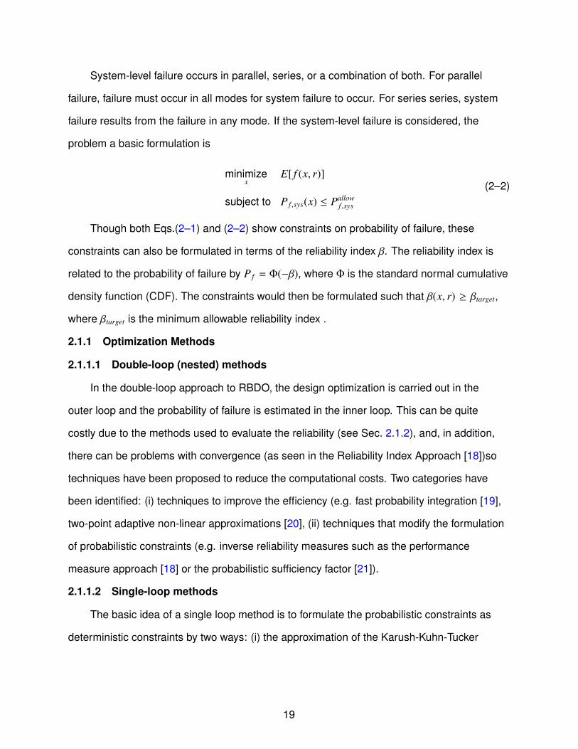
System-level failure occurs in parallel, series, or a combination of both. For parallel

failure, failure must occur in all modes for system failure to occur. For series series, system

failure results from the failure in any mode. If the system-level failure is considered, the

problem a basic formulation is

minimizex

E[ f (x, r)]

subject to P f ,sys(x) ≤ Pallowf ,sys

(2–2)

Though both Eqs.(2–1) and (2–2) show constraints on probability of failure, these

constraints can also be formulated in terms of the reliability index β. The reliability index is

related to the probability of failure by P f = Φ(−β), where Φ is the standard normal cumulative

density function (CDF). The constraints would then be formulated such that β(x, r) ≥ βtarget,

where βtarget is the minimum allowable reliability index .

2.1.1 Optimization Methods

2.1.1.1 Double-loop (nested) methods

In the double-loop approach to RBDO, the design optimization is carried out in the

outer loop and the probability of failure is estimated in the inner loop. This can be quite

costly due to the methods used to evaluate the reliability (see Sec. 2.1.2), and, in addition,

there can be problems with convergence (as seen in the Reliability Index Approach [18])so

techniques have been proposed to reduce the computational costs. Two categories have

been identified: (i) techniques to improve the efficiency (e.g. fast probability integration [19],

two-point adaptive non-linear approximations [20], (ii) techniques that modify the formulation

of probabilistic constraints (e.g. inverse reliability measures such as the performance

measure approach [18] or the probabilistic sufficiency factor [21]).

2.1.1.2 Single-loop methods

The basic idea of a single loop method is to formulate the probabilistic constraints as

deterministic constraints by two ways: (i) the approximation of the Karush-Kuhn-Tucker

19

optimality conditions at the most probable point [22], (ii) finding approximations of proba-

bilistic design through deterministic design [23–25]. Du and Chen developed the sequential

optimization and reliability assessment method (SORA), which uses the information from the

reliability assessment to shift the boundaries of violated constraints to the feasible region

[26].

2.1.2 Methods to Evaluate Reliability

Failure is defined by a limit state function g, which is a function of the design variables x

and the random variables r. It is often defined as the difference between the response R and

capacity C defined for a failure mode. The limit state function can be expressed as

g(x, r) = C(x, r) − R(x, r) (2–3)

where R and C are both functions of both the design and random variables. Failure occurs

when the response exceeds the capacity (g < 0). The probability of failure can be expressed

as

P f = P(g(R) < 0) =∫. . .

∫g(R)<0

fR(R)dX (2–4)

where fR(R) is the joint probability density function for the vector R that contains the random

variables r. As Melchers explains, the analytical calculation of this expression is challenging

because the joint probability density function fR(R) is not usually easily obtained, and, for the

cases when it is obtained, the integration over the failure domain is not easy. Moment and

simulation based methods were developed to calculate the probability of failure.

2.1.2.1 Moment based methods

In moment based methods, the vector of variables is mapped to an independent stan-

dard normal space (known as u-space) by a transformation. Different transformations exist

(e.g., Nataf transformation), but a common transformation is the Rosenblatt transformation

[3, 27]. Moment based methods of calculating the reliability have the advantage of being

generally cheaper than other methods. However, they can only evaluate the probability of

failure of a single mode.

20

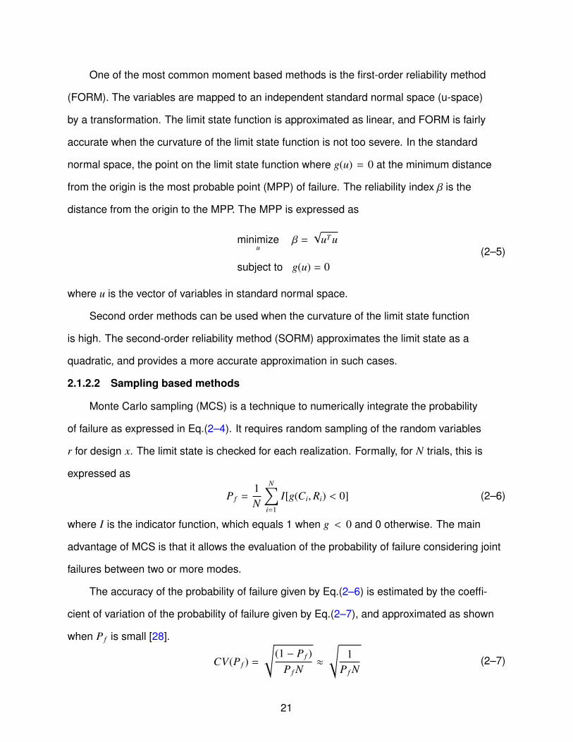
One of the most common moment based methods is the first-order reliability method

(FORM). The variables are mapped to an independent standard normal space (u-space)

by a transformation. The limit state function is approximated as linear, and FORM is fairly

accurate when the curvature of the limit state function is not too severe. In the standard

normal space, the point on the limit state function where g(u) = 0 at the minimum distance

from the origin is the most probable point (MPP) of failure. The reliability index β is the

distance from the origin to the MPP. The MPP is expressed as

minimizeu

β =√

uT u

subject to g(u) = 0(2–5)

where u is the vector of variables in standard normal space.

Second order methods can be used when the curvature of the limit state function

is high. The second-order reliability method (SORM) approximates the limit state as a

quadratic, and provides a more accurate approximation in such cases.

2.1.2.2 Sampling based methods

Monte Carlo sampling (MCS) is a technique to numerically integrate the probability

of failure as expressed in Eq.(2–4). It requires random sampling of the random variables

r for design x. The limit state is checked for each realization. Formally, for N trials, this is

expressed as

P f =1N

N∑i=1

I[g(Ci,Ri) < 0] (2–6)

where I is the indicator function, which equals 1 when g < 0 and 0 otherwise. The main

advantage of MCS is that it allows the evaluation of the probability of failure considering joint

failures between two or more modes.

The accuracy of the probability of failure given by Eq.(2–6) is estimated by the coeffi-

cient of variation of the probability of failure given by Eq.(2–7), and approximated as shown

when P f is small [28].

CV(P f ) =

√(1 − P f )

P f N≈

√1

P f N(2–7)

21

By this approximation, it is seen that, for a probability of failure of 1e-6, 100 million simula-

tions are needed to achieve 10% accuracy for one-sigma level of confidence. Clearly, when

the calculation of the limit state involves complex analyses, such as finite element models,

the accurate calculation of small probabilities of failure becomes expensive.

Smarslok et al. developed the separable Monte Carlo method (SMC) to reformulate the

limit state when the types of uncertainty in the limit state (i.e. response and capacity) are

independent [28]. In separable Monte Carlo, the number of simulations of the response and

capacity can be different, such that an expensive response can be evaluated a fewer number

of times.

P f =1

MN

N∑i=1

M∑j=1

I[g(C j,Ri) < 0] (2–8)

2.2 Definition of Types of Uncertainty

Many have attempted to identify and classify different types of uncertainty that should be

considered in a reliability assessment. A broad and often used classification of uncertainties

categorizes uncertainty as either aleatory (or intrinsic) or epistemic [1, 2]. The terms

“aleatory” and “epistemic” are often used interchangeably with “variability” and “error” ,

respectively.

Aleatory uncertainty generally refers to inherent uncertainties, such as those associated

with physical properties of materials or the environment [3]. Some examples include the

variations in the yield strength of a material, applied loads, or geometric dimensions of

a component. Variability can be reduced with more data (e.g. more tests to reduce the

variation of the yield strength of a material), or quality control (e.g. improved quality control to

reduce variations in dimensions).

Epistemic uncertainty, or error, arises due to lack of knowledge. It is often associated

with the inability to adequately characterize a phenomenon by use of models, such as finite

element models, or through experiments. Epistemic uncertainty can often by reduced by

22

simply adding more knowledge by more research, expert consultation, and tests to calibrate

analytical models, for example.

2.3 Uncertainty Reduction Methods in Reliability Based Design

After design, it is customary for the component to undergo various uncertainty reduction

measures (URMs) followed by remediation, such as redesign or repair, if necessary. Exam-

ples of URMs in the aerospace field include thermal and structural testing, inspection, health

monitoring, maintenance, and improved analysis and failure modeling.

In recent years, there has been a movement to quantify the effect of URMs on the safety

of the product over its life cycle. Much work has been completed in the areas of inspection

and maintenance for structures under fatigue loading. Fujimoto et al. [4], Toyoda-Makino

[5], and Garbatov et al. [6] developed methods to optimize inspection schedules for a given

structural design to maintain a specific level of reliability. Even further, Kale et al. [7, 29]

explored how simultaneous design of the structure and inspection schedule allows the

trading of cost of additional structural weight against inspection cost of stiffened panels

affected by fatigue crack growth.

There have been few studies that have incorporated the effects of future tests followed

by possible redesign on the design of a structure. Studies by Acar et al. [2, 30] investigated

the effects of future tests and redesign on the final distribution of failure stress and structural

design with varying numbers of tests at the coupon, element, and certification levels. Such

studies showed that these tests with possible redesign can greatly reduce the probability

of failure of a structure, and estimated the required structural weight to achieve the same

reduction without tests. Sankararaman et al. [8] proposed an optimization algorithm of test

resource allocation for multi-level and coupled systems.

2.4 The Role of Surrogates

Surrogate models, or meta-models, are often used to reduce the cost associated with

expensive function evaluations, such as those from finite element analysis or computational

fluid dynamics. Some examples of surrogates include polynomial response surfaces

23

[31, 32], kriging [33–35], support vector regression [36], and neural networks [37, 38]. In

optimization, surrogates are often used to provide approximations of the objective function

and/or constraints in optimization. The use of surrogates has been well documented, and for

a complete review surrogates and surrogate-based optimization techniques, the reader is

referred to references [39–43].

Traditional surrogate-based optimization progresses in iterations, or cycles, until an

optimum or suitable solution is found. In one cycle, data from expensive simulations is fit to a

surrogate, the surrogate is used to find a candidate optimum, and the optimum is evaluated

by the expensive simulator. The optimum is generally added to the surrogate in the next

iteration.

In recent years, many have proposed strategies for using multiple surrogates for opti-

mization [9–12]. Viana explains that the use of multiple surrogates over a single surrogate

makes sense because “(i) no single surrogate works well for all problems, (ii) the cost of

constructing multiple surrogates is often small compared to the cost of simulations, and (iii)

use of multiple surrogates reduces the risk associated with poorly fitted models” [39]. In

particular, the ability of multiple surrogates to give different interpretations (i.e., predictions

and uncertainty estimates) of the same design space is attractive.

Multiple surrogates have been used to simply compare the multiple solutions given by

each surrogate. For example, Samad et al. [10] compared polynomial response surface,

kriging, radial basis neural network, and a weighted average surrogate in the shape optimiza-

tion of a compressor blade, and found that the most accurate surrogate did not lead to the

best solution. Zerpa et al. [44] showed that the use of multiple surrogates helped to identify

alternative optimal solutions corresponding to different regions in the design space.

Multiple surrogate techniques include using an ensemble of surrogates, where the

prediction is a weighted result of the surrogate predictions [45–47]. The weights placed on

each surrogate prediction are generally based on local or global error metrics. Proposed

24

methods for choosing the weight factors include error correlation, cross-validation error,

prediction variance, and error minimization.

The addition of multiple points per optimization cycle has also been explored [48–50].

Viana and Haftka and later Chaudhuri et al. developed an algorithm for adding several

points per optimization cycle based on approximated computation of the probability of

improvement (the probability of being below a target value) [13, 51]. Comparing their results

with traditional sequential based optimization with kriging, they were able to deliver better

results in a fraction of the optimization cycles using this algorithm.

2.5 Integrated Thermal Protection System Test Case Description

This section describes the main test case that is used to illustrate the methodologies

presented in this proposal. The integrated thermal protection system was used as an

illustrative example in the articles in Refs. [52–57].

2.5.1 Integrated Thermal Protection System

Large portions of the exterior surface of many space vehicles are devoted to providing

protection from the severe aerodynamic heating experienced during ascent and atmospheric

reentry. Traditionally, thermal protection systems (TPS) do not provide structural support

functions, and are added to only to protect the underlying structure, thereby adding to the

launch weight. This is the case with the TPS of the Apollo, Space Shuttle Orbiter, and X-33

VentureStar. A proposed integrated thermal protection system (ITPS) provides structural

load bearing function in addition to its insulation function, and in so doing provides a chance

to reduce launch weight.

One proposed ITPS design is the corrugated core sandwich structure, which is illus-

trated in Fig. 2-1. This design evolved from studies for reusable launch vehicles (RLV) and

evolved towards robust metallic TPS concepts [58–60], which been the subject of several

studies [61–63]. These studies have shown that this design should be an adequately robust,

weight-efficient, load-bearing structure.

25

Figure 2-1. Corrugated core sandwich panel ITPS concept

The design consists of a top face sheet and webs made of titanium alloy (Ti-6Al-4V),

and a bottom face sheet made of beryllium (grade S200-F, vacuum hot pressed). Saffil R⃝

foam is used as insulation between the webs. The material properties are assumed to

be normally distributed (with the exception of the density of the insulation foam), with the

nominal values and coefficient of variations given in Table 2-1.

Table 2-1. ITPS material propertiesProperty Symbol Nominal CV(%)density of titanium1 ρTi 4429 kg

m3 2.89density of beryllium2 ρBe 1850 kg

m3 2.89density of foam ρS 24 kg

m3 0thermal conductivity of titanium kTi 7.6 W

m/K 2.89thermal conductivity of beryllium kBe 203 W

m/K 3.66thermal conductivity of foam kS 0.105 W

m/K 2.89specific heat of titanium cTi 564 J

kg/K 2.89specific heat of beryllium cBe 1875 J

kg/K 2.89specific heat of foam cS 1120 J

kg/K 2.89

1 Top face sheet and web material2 Bottom face sheet material

The relevant geometric variables of the ITPS design are also shown on the unit cell in

Fig. 2-1. The variables considered are the top face thickness (tT ), bottom face thickness (tB),

thickness of the foam (dS ), web thickness (tw), corrugation angle (θ), and length of unit cell

(2p).

26

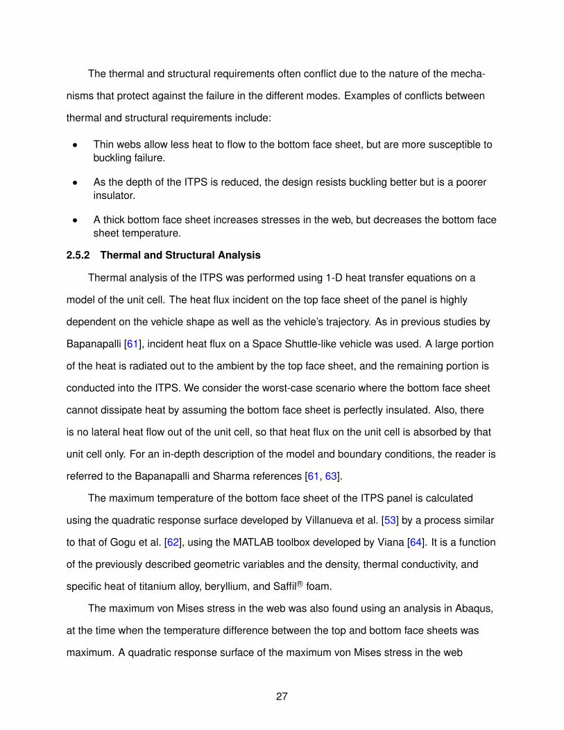
The thermal and structural requirements often conflict due to the nature of the mecha-

nisms that protect against the failure in the different modes. Examples of conflicts between

thermal and structural requirements include:

• Thin webs allow less heat to flow to the bottom face sheet, but are more susceptible tobuckling failure.

• As the depth of the ITPS is reduced, the design resists buckling better but is a poorerinsulator.

• A thick bottom face sheet increases stresses in the web, but decreases the bottom facesheet temperature.

2.5.2 Thermal and Structural Analysis

Thermal analysis of the ITPS was performed using 1-D heat transfer equations on a

model of the unit cell. The heat flux incident on the top face sheet of the panel is highly

dependent on the vehicle shape as well as the vehicle’s trajectory. As in previous studies by

Bapanapalli [61], incident heat flux on a Space Shuttle-like vehicle was used. A large portion

of the heat is radiated out to the ambient by the top face sheet, and the remaining portion is

conducted into the ITPS. We consider the worst-case scenario where the bottom face sheet

cannot dissipate heat by assuming the bottom face sheet is perfectly insulated. Also, there

is no lateral heat flow out of the unit cell, so that heat flux on the unit cell is absorbed by that

unit cell only. For an in-depth description of the model and boundary conditions, the reader is

referred to the Bapanapalli and Sharma references [61, 63].

The maximum temperature of the bottom face sheet of the ITPS panel is calculated

using the quadratic response surface developed by Villanueva et al. [53] by a process similar

to that of Gogu et al. [62], using the MATLAB toolbox developed by Viana [64]. It is a function

of the previously described geometric variables and the density, thermal conductivity, and

specific heat of titanium alloy, beryllium, and Saffil R⃝ foam.

The maximum von Mises stress in the web was also found using an analysis in Abaqus,

at the time when the temperature difference between the top and bottom face sheets was

maximum. A quadratic response surface of the maximum von Mises stress in the web

27

was developed as a function of the geometry, Young’s modulus, Poisson’s ratio, and the

coefficient of thermal expansion. The overall buckling of the web is assumed to be Euler

buckling. It is modeled as a function of the web thickness and width of the foam, along with

the coefficient of thermal expansion and Young’s modulus of the web material to represent a

load due to the temperature difference between the top and bottom.

The mass per unit area m of the ITPS is calculated using Eq.(2–9) where ρT , ρB, and ρw

are the densities of the materials that make up the top face sheet, bottom face sheet, and

web, respectively.

m = ρT tT + ρBtB +ρwtwdS

p sin θ(2–9)

28

CHAPTER 3INCLUDING THE EFFECT OF FUTURE TESTS AND REDESIGN IN RELIABILITY

CALCULATIONS

It is common to test components after they are designed and redesign if necessary. The

reduction of the uncertainty in the probability of failure that can occur after a test is usually

not incorporated in reliability calculations at the design stage. This reduction in uncertainty

is accomplished by additional knowledge provided by the test and by redesign when the test

reveals that the component is unsafe or overly conservative. In this chapter, we develop a

methodology to estimate the effect of a single future thermal test followed by redesign, and

model the effect of the resulting reduction of the uncertainty in the probability of failure. Using

assumed distributions of computation and experimental errors and given re-design rules, we

obtain possible outcomes of the future test and redesign through Monte Carlo sampling to

determine what changes in probability of failure, design, and weight will occur. In addition,

Bayesian updating is used to gain accurate estimates of the probability of failure after a test.

These methods are demonstrated through a future thermal test on an integrated thermal

protection system. We observe that performing redesign following a single future test can

reduce the probability of failure by orders of magnitude, on average, when the objective of

the redesign is to restore original safety margins. Redesign for a given reduced probability of

failure allows additional weight reduction.

3.1 Motivation for Examining Future Tests and Redesign

Traditionally, aerospace structures have been designed deterministically, employing

safety margins and safety factors to protect against failure. After the design stage, most

components undergo tests, whose purpose is to validate the model and catch unacceptable

designs and redesign them. After production, inspection and manufacturing are done to en-

sure safety throughout the lifecycle. In contrast, probabilistic design considers uncertainties

to calculate the reliability, which allows the trade-off of cost and performance.

In recent years, there has been a movement to quantify the effect of uncertainty

reduction measures, such as tests, inspection, maintenance, and health monitoring, on

29

the safety of a product over its life cycle. Much work has been completed in the areas of

inspection and maintenance for structures under fatigue [4–7]. Studies by Acar et al. [2]

investigated the effects of future tests and redesign on the final distribution of failure stress

and structural design with varying numbers of tests at the coupon, element, and certification

levels. Golden et al. [65] proposed a method to determine the optimal number of experiments

required to reduce the variance of uncertain variables. Sankararaman et al. [8] proposed

an optimization algorithm of test resource allocation for multi-level and coupled systems.

A method to simultaneously design a structural component and the corresponding proof

test considering the probability of failure and the probability of failing the proof test was

introduced by Venter and Scotti [66].

Most aerospace components are designed using a computational modeling technique,

such as finite element analysis. We expect some error, often labeled as epistemic uncer-

tainty (associated with lack of knowledge), in the modeled behavior. The true value of this

error is unknown, and thus we consider this lack of knowledge to lead to an uncertain future.

Tests are performed to reduce the error, thus narrowing the range of possible futures through

the knowledge gained and the correction of unacceptable futures by redesign.

In this study, we examine the effect of a single future thermal test followed by possible

redesign on the reliability and weight of an integrated thermal protection system (ITPS).

A description of the integrated thermal protection system is presented in Sec. 2.5.1. An

experiment that finds the bottom face sheet temperature of a small ITPS panel is usually

conducted in a vacuum chamber with heat applied to the top face sheet by heat lamps. The

sides of the panel are typically surrounded by some kind of insulation to prevent lateral heat

loss. The temperature of the bottom face sheet is found with thermocouples embedded into

or in contact with the lower surface of the bottom face sheet. The thermal test considered

in this study measures the maximum temperature of the bottom face sheet, which is critical

due to its proximity to the underlying vehicle structure. A design is considered to have failed

thermally if it exceeds the maximum allowable temperature.

30

In previous work on the optimization of the ITPS, Villanueva et al. [53] used probability of

failure calculations that considered only the variability in geometric and material parameters

and error due to shortcomings in the analytical model. Expanding on those studies, we

include the information gained from a test in a temperature estimate, the reduction in

uncertainty resulting from the test, and the ability of the test to guide redesign for dangerous

or overly conservative designs. Thereby, the objective of this chapter is to:

1. Present a methodology to both predict and include the effect of a future redesignfollowing a test during the design stage

2. Illustrate the ability of a test in combination with redesign to reduce the probability offailure even when a test shows that the design is computationally unconservative

3. Examine the overall changes in mass resulting from redesign based on the future test

The uncertainty model and probability of failure calculations are described in Section

3.2. Section 3.3 continues with the methodology to calibrate the computational model based

on a test and includes redesign based on the test. The method to simulate future tests is

summarized in Section 3.4. Section 3.5 presents an illustrative example that details the effect

of including the test and redesign in probability of failure calculations.

3.2 Uncertainty Modeling

3.2.1 Classification of Uncertainties

Oberkampf et al. [1] provided an analysis of different sources of uncertainty in engineer-

ing modeling and simulation, which was simplified by Acar et al. [2]. We use classification

similar to Acar’s to categorize types of uncertainty as errors (uncertainties that apply equally

to every ITPS) or variability (uncertainties that vary in each individual ITPS). We further

describe errors as epistemic and variability as aleatory. As described by Rao et al. [67], the

separation of the uncertainty into aleatory and epistemic uncertainties allows more under-

standing of what is needed to reduce the uncertainty. Tests reduce errors by allowing us to

calibrate analytical models. For example, testing can be done to reduce the uncertainty in

failure predictions due to high stresses. Variability can be reduced by lowering tolerances in

31

manufacturing. Variability is modeled as random uncertainties that can be modeled proba-

bilistically. In contrast, errors are fixed for a given ITPS and are largely unknown, but here

they are modeled probabilistically as well.

Variability in material properties and construction of the ITPS leads to variability in

the ITPS thermal response. More specifically, we will have variability in the calculated

temperature due to the input variabilities. We simulate this process with a Monte Carlo

simulation (MCS) that generates values of the random variables r based on an estimated

distribution and calculates the bottom face sheet temperature Tcalc for each, generating the

probability distribution function. The calculated temperature distribution that reflects the

random variability is denoted fcalc(T ). In estimating the probability of failure, we also need to

account for the modeling or computational error. We denote this computational error by ec,

where ec is modeled as a uniformly distributed random variable within confidence limits the

in the computational model as defined by the analyst. Unlike the variability, the error has a

single value, and the uncertainty is due to our lack of knowledge.

For a given design given by d and r, the possible true temperature TPtrue can be found by

Eq.(3–1) in terms of possible computational errors ec. The sign in front of ec is negative so a

positive error implies a conservative calculation, meaning it overestimates the temperature.

TPtrue(d, r, ec) = Tcalc(d, r)(1 − ec) (3–1)

Since the analyst does not know ec and it is modeled as a random variable, we can

form a distribution of the possible true temperature, denoted as fPtrue(T ). To illustrate

the difference between the true distribution of the temperature ftrue(T ) and possible true

distribution fPtrue(T ), let us consider a simple example where the calculated temperature

of the nominal design is 1, the true temperature is 1.05, and the computational error is

uniformly distributed in the range [-0.1,0.1]. The possible true temperature without variability

are uniformly distributed in [0.9,1.1] by Eq.(3–1). Now, let us consider an additional variability

in the temperature due to manufacturing tolerances in the range [-0.02, 0.01], such that

32

Tcalc(d, r) is uniformly distributed in the range [0.98,1.01]. Finally, the true temperature will

vary from [1.03,1.06] as ftrue(T ), and the possible true temperature from [0.882, 1.111] as

fPtrue(T ).

Figure 3-1 illustrates how we arrive at the distribution fPtrue(T ). The input random

variables have initial distributions, denoted as finp(r), and these random variables, in

combination with the design variables, lead to the distribution of the calculated temperature

fcalc(T ). The random computational error is applied, leading to the distribution of the possible

true temperature fPtrue(T ), which has a wider distribution than fcalc(T ).

Figure 3-1. Illustration of the variability of the input random variables, calculated value,computational error, and resulting distribution of possible true temperature

As previously noted, ec is modeled as a random variable not because it is random,

but because its value is unknown to the analyst. To emphasize this point, the actual true

temperature is known only when we know the actual value of ec as ec,true as illustrated in

Eq.(3–2).

Ttrue(d, r) = Tcalc(d, r)(1 − ec,true) (3–2)

Again, these true values are unknown to the analyst. This distinction between true values

and analyst-estimated, possible true values is important and will be a point of comparison

throughout this chapter.

Figure 3-2 shows an example of the probability distribution of the true temperature

ftrue(T ), as well as the probability density functions (pdf) of fcalc(T ) and fPtrue(T ). For this

example, we modeled the variability in the material properties and variability in geometry

33

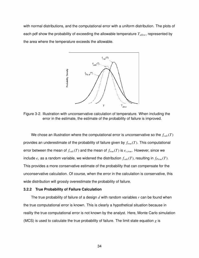
with normal distributions, and the computational error with a uniform distribution. The plots of

each pdf show the probability of exceeding the allowable temperature Tallow, represented by

the area where the temperature exceeds the allowable.

Figure 3-2. Illustration with unconservative calculation of temperature. When including theerror in the estimate, the estimate of the probability of failure is improved.

We chose an illustration where the computational error is unconservative so the fcalc(T )

provides an underestimate of the probability of failure given by ftrue(T ). This computational

error between the mean of fcalc(T ) and the mean of ftrue(T ) is ec,true. However, since we

include ec as a random variable, we widened the distribution fcalc(T ), resulting in fPtrue(T ).

This provides a more conservative estimate of the probability that can compensate for the

unconservative calculation. Of course, when the error in the calculation is conservative, this

wide distribution will grossly overestimate the probability of failure.

3.2.2 True Probability of Failure Calculation

The true probability of failure of a design d with random variables r can be found when

the true computational error is known. This is clearly a hypothetical situation because in

reality the true computational error is not known by the analyst. Here, Monte Carlo simulation

(MCS) is used to calculate the true probability of failure. The limit state equation g is

34

formulated as the difference between a capacity C and response R as shown in Eq.(3–3).

g = Tallow − Ttrue(d, r) ≡ C − R (3–3)

Since we consider failure to occur when the maximum bottom face sheet temperature

exceeds the allowable temperature Tallow, the response is Ttrue and the capacity is the

allowable temperature. The true probability of failure p f ,true is estimated with Eq.(3–4).

p f ,true =1N

N∑i=1

I[g(Ci,Ri) ≤ 0] (3–4)

The indicator function I equals 1 if the response exceeds the capacity, and equals 0 for the

opposite case. The number of samples is N.

3.2.3 Analyst-Estimated Probability of Failure Calculation

Since the true computational error is unknown, the true probability of failure is unknown

as well. Because of this, the best estimate the analyst can obtain uses the calculated

temperature Tcalc and the computational error through the possible true temperature of

Eq.(3–1) to determine the estimated probability of failure with the limit state equation

formulated as in Eq.(3–5).

g = Tallow − TPtrue(d, r, ec) ≡ C − R (3–5)

Since the two types of uncertainty (computational errors and variability in material

properties and geometry) in the response are independent, Separable Monte Carlo (SMC)

sampling[28] can be used when evaluating the probability of failure. The limit state equation

can be reformulated so that the computational error is on the capacity side, and all random

variables associated with material properties and geometry lie on the response side.

g =Tallow

1 − ec− Tcalc(d, r) ≡ C′ − R′ (3–6)

This analyst-estimated probability of failure p f ,analyst can then be calculated with Eq.(3–7),

where M and N are the number of capacity and response samples, respectively.

35

p f ,analyst =1

MN

N∑i=1

M∑j=1

I[g(C j,Ri) ≤ 0] (3–7)

3.3 Including the Effect of a Calibration Test and Redesign

We consider a test, performed for the purpose of validating and calibrating a model,

for a selected design dtest to determine the temperature of the test article Ttest. We further

assume that the test article is carefully measured for both dtest and rtest so that both are

accurately known, and that the errors in the computed temperatures due to uncertainty in the

values of dtest and rtest are small compared to the measurement errors and can be neglected.

If no errors are made in the measurements of dtest, rtest, and Ttest, then the experimental result

is actually the true temperature of the test article. We denote this error-free test temperature

Ttest,true.

Ttest,true = Ttrue(dtest, rtest) (3–8)

However, there is unknown measurement error ex, which we model as a random

variable based on our estimate of the accuracy of the test. The measured temperature Tmeas

then includes the experimental error ex,true. The experimental error could also include a

component due to the fact that rtest is not perfectly known.

Tmeas =Ttest,true

1 − ex,true(3–9)

Using the computational and experimental results, along with the corresponding error

estimates for the test article, we are able to refine the calculated value and its error for any

design described by the design variables d and random variables r. In this way, the result

of the single test can be used to calibrate calculations for other designs. We examine two

methods, which take different approaches in using the test as calibration. The first approach

introduces a simple correction factor based on the test result. The second uses the Bayesian

method to update the uncertainty of the calculated value for dtest based on the test result and

then transfers this updated uncertainty to other calculations as the means of calibration.

36

3.3.1 Correction Factor Approach

The correction factor approach is a fairly straightforward method of calibration. Assum-

ing that the test result is more accurate than the calculated result for the test article, we scale

Tcalc for any value of d and r by the ratio of the test result to the calculated result to obtain the

corrected calculation Tcalc,corr.

Tcalc,corr = Tcalc(d, r)(

Tmeas

Tcalc(dtest, rtest)

)(3–10)

3.3.2 Bayesian Updating Approach

Before the test, we have an expectation of the test results based on the computational

result of dtest and rtest. We denote this distribution by f initest,Ptrue, which can be viewed as the

distribution of fPtrue(T ) of the test article with fixed random variables rtest. Furthermore, it may

be viewed as the possible true temperature distribution of the test article just before the test.

In the test, we measure a temperature Tmeas. Because of experimental error ex, the true

test result Ttest,true is not equal to Tmeas (as seen in Eq.(3–9)). The possible true value of the

test result is instead given as

T meastest,Ptrue = Tmeas(1 − ex) (3–11)

where T meastest,Ptrue forms the distribution of possible true test results available from the measure-

ments only. We thus have two distributions of possible true test results. One is based on the

calculated value and the distribution of the calculation error, and the other is based on the

measurement and the distribution of the measurement error.

The Bayesian approach combines these two distributions to obtain a narrower and more

informative distribution. In this formulation, the probability distribution of the possible true

temperature of the test article ftest,Ptrue(T ) is updated as

f updtest,Ptrue(T ) =

ltest(T ) f initest,Ptrue(T )∫ +∞

−∞ ltest(T ) f initest,Ptrue(T )dT

(3–12)

37

where the likelihood function ltest(T ) is the conditional probability density of obtaining the test

result Tmeas when the true temperature of the test article is T . That is, ltest is the probability

density of T1−ex

evaluated at T = Tmeas.

The updated estimate f updtest,Ptrue(T ) is the distribution of the updated true possible

test result T updtest,Ptrue. This is used to find the distribution of the Bayesian estimate of the

computational error eBayes with Eq.(3–13).

eBayes = 1 −T upd

test,Ptrue

Tcalc(dtest, rtest)(3–13)

We can then replace the possible true temperature given by Eq.(3–1) with a true

temperature that uses the Bayesian estimate of the error.

TPtrue(d, r, eBayes) = Tcalc(d, r)(1 − eBayes)(1 − eextrap) (3–14)

The additional error eextrap is included to account for the error that occurs when applying this

Bayesian estimate of the error to some design other than the test design. This extrapolation

error is further described in Sec. 3.3.2.2.

Note that it is also possible to perform the Bayesian updating by reversing the roles of

the two possible true test temperatures. That is, we could take the distribution based on the

measurement error as the initial distribution, and take the computed result as the additional

information. However, in this case the likelihood function would require repeated simulations

for different possible true temperatures, greatly increasing the computational cost.

3.3.2.1 Illustrative example of calibration by the Bayesian approach

To illustrate how Bayesian updating is used to calibrate calculations based on a single

future test, we consider a simple case where both the computational and experimental errors

are uniformly distributed. To simplify the problem, we normalize all temperatures by the

calculated temperature so that Tcalc(dtest, rtest) = 1. The error bound of the calculation is ±10%

and the error bound of the test is ±7%. The normalized test result is Tmeas = 1.05.

38

In this work, we make the simplifying assumption that the likelihood function is about

Tmeas rather than T . That is, we use conditional probability of obtaining the temperature T

given the measured temperature. This allows for a uniform value of the likelihood function

where it is nonzero, which thereby results in a uniform distribution of the updated Bayesian

estimate of the computational error since the distribution of f updtest,Ptrue will also be uniform.

The effect of this approximation of the likelihood function is examined in Appendix A. The

initial probability distribution f initest,Ptrue(T ) and the likelihood function ltest are described by Eqs.

(3–15) and (3–16), respectively.

f initest,Ptrue(T ) =

1

0.2Tcalc(dtest ,rtest)if∣∣∣∣ TTcalc(dtest ,rtest)

− 1∣∣∣∣ ≤ 0.1;

0 otherwise.(3–15)

ltest(T ) =

1

0.14Tmeasif∣∣∣∣T−Tmeas

Tmeas

∣∣∣∣ ≤ 0.07;

0 otherwise.(3–16)

Since Tcalc(dtest) = 1 and the computation error bounds are ±10%, the initial distribution

of the true temperature is f initest,Ptrue(T ) = 5 on the interval (0.9, 1.1) and zero elsewhere. This

is shown in Fig. 3-3. The test result of Tmeas = 1.05 results in a likelihood of ltest = 6.803

on the interval (0.9765, 1.1235) and zero elsewhere. Equation (3–12) is used to find the

updated Ttrue distribution so that f updtest,Ptrue(T ) = 8.1 on the interval (0.9765, 1.1) and zero

elsewhere.

The updated distribution shows that the true temperature is somewhere on the interval

(0.9765, 1.1). Using this temperature distribution along with the calculated value Tcalc(dtest),

the updated error distribution eBayes can be found. Through Eq.(3–13), we determine that

eBayes is uniformly distributed from -10% to 2.35%.

3.3.2.2 Extrapolation error in calibration

Figure 3-4 illustrates how the Bayesian approach is used to calibrate the calculations for

other designs described by d. Here, we consider the case when the calculated temperature

39

Figure 3-3. Illustrative example of Bayesian updating showing the initial distribution (top),initial distribution and test (middle), and updated distribution (bottom).

is linear in the design variable d, and there is no variability (random variables fixed at nominal

values).

Figure 3-4. Illustration of the calibration using Bayesian updating

40

At design dtest, we have the same error scenario similar to that illustrated in Fig. 3-3.

That is, we represent the calculated temperature at dtest as a point on the solid black line,

and the error bounds about this calculation by the dotted black lines. The star represents

the experimentally measured temperature, and the error bars show the uncertainty in

this temperature. By the Bayesian approach, we obtain a corrected test temperature as

represented by the point on the grey line, as well as updated error bounds represented by

the grey dash-dot line.

However, this correction and updated error is most accurate at the test design. There-

fore, we apply an additional error, the extrapolation error eextrap, when calibrating designs

other than dtest. Note that at dtest the updated error bounds in Fig. 3-4 coincide with the error

bounds of the test. As the design becomes increasingly different from dtest, the updated error

bounds become wider.

The magnitude of eextrap is assumed to be proportional the distance between d and dtest,

such that

eextrap = (eextrap)max∥d − dtest∥∆dlim

(3–17)

This defines the extrapolation error so that it is maximum when the distance between d and

dtest is at limit of this distance ∆dlim and zero at the test design. The extrapolation error is a

measure of the variation of the errors in the model away from the test design. In this work,

we assume that the magnitude of eextrap is linear with the distance between d and dtest, which

would be reasonable for small changes in the design. However, we examine the effect of this

assumption in Appendix B where we use a quadratic variation.

3.3.3 Test-Corrected Probability of Failure Estimate

The corrected probability of failure p f ,analyst−corr after the test can be estimated by the

analyst using the updated error obtained from the Bayesian approach. Separable Monte

Carlo is used to calculate p f ,analyst−corr.

g =Tallow

1 − eBayes− Tcalc(d, r)(1 − eextrap) ≡ C − R (3–18)

41

p f ,analyst−corr =1

MN

N∑i=1

M∑j=1

I[g(C j,Ri) ≤ 0] (3–19)

3.3.4 Redesign Based on the Test

Two criteria for redesign are considered, each with different perspectives on the purpose

of the redesign. The first criterion is based on the agreement between the measured and

calculated values for the test article. The second criterion considers the probability of failure

estimated by the analyst.

3.3.4.1 Deterministic redesign

In deterministic redesign, redesign occurs when there is a significant difference between

the experimentally measured temperature Tmeas and the expected temperature given by the

computational model. It is assumed that the temperature given by the computational model

(Tcalc) is the desired value. Therefore, the component is redesigned to restore this original

temperature.

The deterministic redesign criterion is implemented by imposing limits on the acceptable

ratio of the measured temperature to the calculated temperature. Redesign occurs when

TmeasTcalc(dtest ,rtest)

is less than the lower limit DL (conservative computational model) or exceeds the

upper limit DU (unconservative computational model).

3.3.4.2 Probabilistic redesign

In probabilistic redesign, the original structure is designed for a specified probability of

failure, and redesign is also done to achieve a specified probability of failure. It is reasonable

to select the target redesign probability p f ,target to be the same as that obtained with proba-

bilistic design. The target redesign probability of failure can also be set to make the design

safer after the test. Therefore, redesign occurs when the test-corrected probability of failure

estimate, given by Eq.(3–19) is outside the limits of the acceptable range. The lower limit of

this range is denoted PL, and the upper limit PU .

42

3.4 Monte Carlo Simulations of a Future Test and Redesign

Monte Carlo simulations are used to simulate the effect of a future test for a design

described by design variables d and random variables r with the goal of simulating multiple

possible outcomes of this test. To simulate a single outcome of the future test, we first obtain

a single sample of the true computational and experimental errors.

Using the calculated value for the test design and the true computational error, we can

obtain the true temperature by Eq.(3–2). Next, the experimentally measured temperature is

found using Eq.(3–9). The choice can be made to calibrate by the correction factor approach

or the Bayesian updating approach, and, further, the choice of deterministic or probabilistic

redesign can be made.

The true and corrected analyst-estimated probabilities of failure after the test can then

be determined. At this point, the effect of only one possible outcome of the test has been

examined. The major steps and equations involved in the simulation of a single outcome of

the test are summarized in the pseudocode given in Algorithm 1 1 .

To determine another possible outcome, the true computational and experimental errors

are re-sampled and the process is repeated. Therefore, for n possible outcomes of a future

test, we sample n pairs of the errors and true probabilities of failure, n analyst-estimated

probabilities of failure after the test, and up to n updated designs. Note that there is a single

initial design, but if k of the n cases are re-designed we will end up with up to k + 1 different

designs.

3.5 Illustrative Example

In this example, we compare the probabilities of failure of an ITPS with the dimensions

and material properties of probabilistic optimum found in [53]. In that study, the optimum

1 In the implementation of this algorithm, it is assumed that all analysts performing the testhave the same value of rtest. Since each analyst accurately measured rtest,the effect of thisassumption is likely to be negligible.

43

Algorithm 1 Procedure to simulate n possible true computational errors to calculate proba-bility of failure for design d and r, and n possible outcomes of the future test with redesign fora design described by dtest and rtest. The random variables rtest are fixed for the test. The setof samples of r are fixed over the original design and the redesigns.

1: Sample set of values of random variables r (this set is fixed over the n possible out-comes, and for the original design d and any redesigned d)

2: Sample n values of ec and ex

3: Calculate Tcalc(d, r) using computational model and Tcalc,test(dtest, rtest)4: Calculate p f ,analyst by n samples of ec and Eqs. (3–6) and (3–7)5: for i = 1→ n do6: Set ec,true = ec(i) and ex,true = ex(i)7: Calculate p f ,true by Eqs. (3–3) and (3–4)8: Calculate Ttrue,test(dtest, rtest) by Eq. (3–2) and Tmeas by Eq. (3–9)9: if Correction-Factor Calibration then

10: Calculate Tcalc,corr(d, r) by Eq. (3–10)11: else if Bayesian Calibration then12: Calculate eBayes by Eqs. (3–12) and (3–13), and eextrap by Eq. (3–17)13: Update p f ,analyst−corr by n samples of ec and Eqs. (3–18) and (3–19)14: end if15: if Deterministic Redesign then16: if Tmeas

Tcalc(dtest ,rtest)< DL || Tmeas

Tcalc(dtest ,rtest)> DU then

17: Redesign for (Tcalc,corr(d, r))redesign = (Tcalc(d, r))original design

18: Update p f ,true by Eqs. (3–3) and (3–4)19: end if20: else if Probabilistic Redesign then21: if p f ,analyst−corr > p f ,target + PU || p f ,analyst−corr < p f ,target − PL then22: Redesign for p f ,analyst−corr = p f ,target

23: Update p f ,true by Eqs. (3–3) and (3–4)24: Update p f ,analyst−corr by n samples of ec and Eqs. (3–6) and (3–7)25: end if26: end if27: end for

was found with constraints on the maximum bottom face sheet temperature, buckling of the

web, and maximum von Mises stress in the webs with the bottom face sheet, web thickness,

and foam thickness as the design variables. The failure considered here is exceeding the

allowable bottom face sheet temperature Tallow. All random variables are normally distributed

with the mean and coefficient of variation (CV) shown in Table 3-1.

In this example, we consider uniform distributions of the errors, with the experimental

error significantly smaller at ±3% than the computational error at ±10%, as shown in Table

44

Table 3-1. ITPS variablesVariable Symbol Nominal CV(%)web thickness tw 1.77 mm 2.89bottom face sheet tB 7.06 mm 2.89foam thickness ds 71.3 mm 2.89top face sheet thickness tT 1.2 mm 2.89half unit cell length p 34.1 mm 2.89angle of corrugation θ 80◦ 2.89density of titanium1 ρTi 4429 kg

m3 2.89density of beryllium2 ρBe 1850 kg

m3 2.89density of foam ρS 24 kg

m3 0thermal conductivity of titanium kTi 7.6 W

m/K 2.89thermal conductivity of beryllium kBe 203 W

m/K 3.66thermal conductivity of foam kS 0.105 W

m/K 2.89specific heat of titanium cTi 564 J

kg/K 2.89specific heat of beryllium cBe 1875 J

kg/K 2.89specific heat of foam cS 1120 J

kg/K 2.891 Top face sheet and web material2 Bottom face sheet material

3-2. The original estimated probability of failure is 0.12% and the nominal mass per unit area

is 35.1 kg/m2. Since the distributions of the errors are bounded, we remove the possibility

of extreme differences between the calculated and experimentally measured values in

the simulated the future test. With these values of the errors, in the most extreme case,

the temperatures differ by approximately 13%, which occurs when the errors are sampled

at opposing bounds of the distribution (e.g. ec,true = 0.1 and ex,true = −0.03). If normal

distributions of the errors were used, this difference can become infinite.

Table 3-2. Distribution of errorsError Distribution Boundsec Uniform ±10%ex Uniform ±3%

The extrapolation error eextrap is estimated to be 2% when d is changed by ±10% from

dtest, and varies linearly with change in d.

eextrap = 0.02∥d − dtest∥0.1∥dtest∥

(3–20)

45

It is possible to assume other relationships between of the extrapolation error and the

distance of d from dtest. In Appendix B, we examine the effect of assuming the magnitude of

eextrap is quadratic with the change in d.

In this example, we examine the benefits of including a future test by examining several

cases that include future tests, one without redesign and one with redesign based on the

future test by the process described in Section 3.4. We will examine 10,000 possible future

test outcomes (10,000 samples of the errors), and use 10,000 samples of the random

variables. Therefore, the true probability of failure is calculated with 10,000 samples each of

the response and capacity, whereas the analyst-estimated probability of failure is calculated

with 10,000 samples of the capacity and 10,000 of the response by separable Monte Carlo.

To reduce the effect of noise, the set of 10,000 random variables was held constant through

each of the 10,000 possible future test outcomes.

3.5.1 Future Test without Redesign

Using the 10,000 possible outcomes of the single future test, we can estimate the

effectiveness of the Bayesian approach by comparing three cases. In the first case, the

analyst accepts Tcalc as the best estimate of the test article temperature. In the second, the

analyst accepts Tmeas. In the third, the analyst accepts TBayes where TBayes is the temperature

with the maximum likelihood in the updated distribution . Since this example simplifies the

likelihood function (see Section 3.3.2.1) so that the updated distribution is uniform, we take

the mean the distribution as TBayes. We compare the absolute error of each from the true

temperature in Table 3-3.

Table 3-3. Comparing absolute true error when using Tcalc, Tmeas and TBayes as the test articletemperature

T compared Mean error (%) Standard deviation of error (%)Tcalc 5.0 2.9Tmeas 1.5 0.8TBayes 1.3 0.8

These results show that the Bayesian approach provides the analyst with the most

accurate estimate of Ttrue for the test article. Accepting Tmeas results in a slightly increased

46

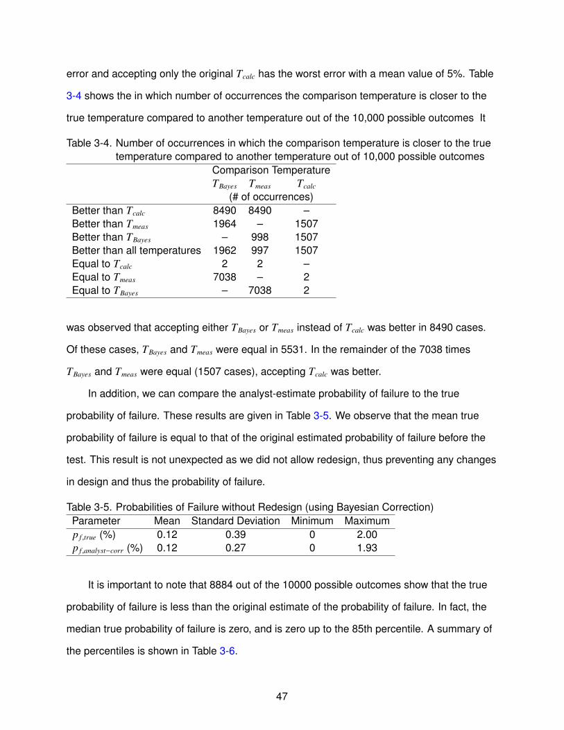
error and accepting only the original Tcalc has the worst error with a mean value of 5%. Table

3-4 shows the in which number of occurrences the comparison temperature is closer to the

true temperature compared to another temperature out of the 10,000 possible outcomes It

Table 3-4. Number of occurrences in which the comparison temperature is closer to the truetemperature compared to another temperature out of 10,000 possible outcomes

Comparison TemperatureTBayes Tmeas Tcalc

(# of occurrences)Better than Tcalc 8490 8490 –Better than Tmeas 1964 – 1507Better than TBayes – 998 1507Better than all temperatures 1962 997 1507Equal to Tcalc 2 2 –Equal to Tmeas 7038 – 2Equal to TBayes – 7038 2

was observed that accepting either TBayes or Tmeas instead of Tcalc was better in 8490 cases.

Of these cases, TBayes and Tmeas were equal in 5531. In the remainder of the 7038 times

TBayes and Tmeas were equal (1507 cases), accepting Tcalc was better.

In addition, we can compare the analyst-estimate probability of failure to the true

probability of failure. These results are given in Table 3-5. We observe that the mean true

probability of failure is equal to that of the original estimated probability of failure before the

test. This result is not unexpected as we did not allow redesign, thus preventing any changes

in design and thus the probability of failure.

Table 3-5. Probabilities of Failure without Redesign (using Bayesian Correction)Parameter Mean Standard Deviation Minimum Maximump f ,true (%) 0.12 0.39 0 2.00p f ,analyst−corr (%) 0.12 0.27 0 1.93

It is important to note that 8884 out of the 10000 possible outcomes show that the true

probability of failure is less than the original estimate of the probability of failure. In fact, the

median true probability of failure is zero, and is zero up to the 85th percentile. A summary of

the percentiles is shown in Table 3-6.

47

Table 3-6. Summary of the percentiles of the true probability of failure without redesignPercentiles

25% 50% 75% 88.8% 90% 95% 97.5%p f ,true (%) 0 0 0 0.15 0.20 1.10 1.80

Based on the large number of true probability of failures that are zero, it would be

expected that if redesign were implemented to restore the original estimated probability of

failure, most redesigns would increase the probability of failure.

3.5.2 Redesign Based on Test

In this section, we examine the effect of deterministic and probabilistic redesign for the

example. These two redesign methodologies are described in Sec. 3.3.4.

3.5.2.1 Deterministic redesign

We chose deterministic redesign to occur when the ratio TmeasTcalc(dtest ,rtest)

is greater than 1.05

(unconservative computational model) or less than 0.95 (conservative computational model).

We consider one design variable, the foam thickness ds. This variable was chosen since it

has a large impact on the bottom face sheet temperature. The results including deterministic

redesign are given in Table 3-7.

Table 3-7. Calibration by the correction factor approach with deterministic redesign.Parameter Original Mean Standard Deviation Minimum MaximumdS (mm) 71.3 71.5 1.2 44.8 99.4mass (kg/m2) 35.1 35.1 2.8 28.9 41.6p f ,true (%) 0.12 0.000712 0.009 0 0.201 Of the 10000 possible outcomes of the future test, 4964 required redesign.

Conservative cases account for 2425 of the redesigns, and unconservativecases account for 2539.

2 99.3% of true probability failures are below the mean.

These results show that the true probability of failure is greatly reduced when redesign

is allowed. In addition, the standard deviation is also reduced. Since the redesign is sym-

metric, it does not cause much change in the average mass. The reason for this drastic

reduction in probability of failure is the substantial reduction in error that allowed us to re-

design all the designs that had a probability of failure above 0.12%. So while the system was

48

designed for a probability of failure of 0.12%, it ended up with a mean probability of failure of

0.0007%.

However, we note a large standard deviation in ds, with the minimum and maximum

values quite different from the design value of 71.3 mm. In practice, the redesign may not

be allowed to be this drastic. Therefore, we also examine the case where the bounds of the

redesigned ds are restricted to ±10% of the original nominal dS . These results are given in

Table 3-8.

Table 3-8. Calibration by correction factor with deterministic redesign, bounds of redesignedds restricted to ±10% of original ds

Parameter Original Mean Standard Deviation Minimum MaximumdS (mm) 71.3 71.4 0.5 64.1 78.4mass (kg/m2) 35.1 35.1 1.2 33.4 36.7p f ,true (%) 0.12 0.0007 0.009 0 0.20

We observe that restricting the bounds of dS does not change the true probability of failure,

and does not cause a significant change in the average mass.

3.5.2.2 Probabilistic redesign

The initial design does not necessarily meet the reliability requirements of the designer.

It can be, for example, a candidate design in a process of design optimization. When it

comes to probabilistic redesign, one may examine re-design to the mean probability without

redesign or to a target probability. Here we assume the latter, and we examine cases where

the target redesign probability is p f ,target = 0.01% with and without bounds on ds. Here, we

require redesign to occur when the estimated probability of failure is not within ±50% of the

target. We require that all unconservative (dangerous) designs above the 50% threshold be

redesign but reject the redesign of overly conservative cases if its mass does not decrease

by at least 4.5%. Since only one design variable, the foam thickness, is considered, a

decrease in mass can only result from a decrease in foam thickness, which causes an

increase in temperature. The results are shown in Table 3-9.

49

Without bounds on the redesigned ds, we observe that the analyst-estimated target

probability of failure is close to the target of 0.01%. It is also observed that there is a signif-

icant reduction in mass (4% reduction) and a reduction in the original mean true probability

of failure from 0.12% to 0.003%. The analyst is able to estimate this true probability of failure

with reasonable accuracy.

When we include the bounds on ds, the true probability of failure is unable to converge

to the target probability of failure, but there is better agreement between the analyst-

estimated probabilities of failure and the true value. This is due to the inclusion of the

extrapolation error in the probability of failure in the redesign process. We also observe a

1.7% reduction in mean mass from the original value.

On a final note, we recognize that the large percentage of redesigns is undesirable. This

percentage can be greatly reduced by less stringent redesign rules while still having very low

probabilities of failure.

3.6 Summary and Concluding Remarks

This study presented a methodology to include the effect of a single future test followed

by redesign on the probability of failure of an integrated thermal protection system. Two

methods of calibration and redesign based on the test were presented. We observed that

the deterministic approach, which represents current design/redesign practices, leads to a

greatly reduced probability of failure after the test and redesign, a reduction that usually is

not quantified.

The probabilistic approach includes the Bayesian technique for calibrating the temper-

ature calculation and re-design to a target probability of failure. It provides a way to more

accurately estimate the true probability of failure after the test. In addition, it allows us to

trade weight against performing additional tests.

Though the methodology is presented in the context of a future thermal test and

redesign on the ITPS, the methodology is applicable for estimating the reliability of almost

any component that will undergo a test followed by possible redesign. Given a computational

50

model, uncertainties, errors, and redesign procedures, along with the statistical distributions,

the procedure of simulating the future test result by Monte Carlo sampling, calibration, and

redesign can be readily applied.

This study brought to light many tunable parameters in the test, such as the bounds on

the design variables, the target probability of failure for redesign, and the redesign criterion

itself. By including these parameters into the optimization, we will not only optimize the

design but optimize the test as well. This work is the focus of Ch. 4.

51

Table 3-9. Calibration by the Bayesian updating approach with probability of failure based redesign(p f ,target = 0.01%)

Restriction on redesigned ds Parameter Original Mean Standard Deviation Minimum Maximum

No bounds

dS (mm) 71.3 65.3 8.9 47.5 77.7mass (kg/m2) 35.1 33.7 2.1 29.5 36.5p f ,true (%) 0.12 0.00312 0.016 0 0.100p f ,analyst−corr (%) 0.12 0.007 0.004 0 0.015

Within ±10% of dtest


1 Of the 10,000 possible outcomes of the future test, 7835 are redesigned. With the requirement of a 4.5%decrease in mass, 5126 of the 7001 conservative models (p f ,analyst < p f ,target) are redesigned. For unconser-vative designs, 2709 are redesigned.

2 97.4% of true probabilities of failure are below the mean.

52

CHAPTER 4ACCOUNTING FOR FUTURE REDESIGN TO BALANCE PERFORMANCE AND

DEVELOPMENT COSTS

As seen in the previous chapter, most components undergo tests after they are de-

signed and are redesigned if necessary. Tests help designers find unsafe and overly con-

servative designs, and redesign can restore safety or increase performance. In general, the

expected changes to the performance and reliability of the design after the test and redesign

are not considered. In this chapter, we explore how modeling a future test and redesign

provides a company an opportunity to balance development costs versus performance by

simultaneously designing the design and the post-test redesign rules during the initial design

stage. Due to regulations and tradition, safety margin and safety factor based design is

common practice in industry as opposed to probabilistic design. In this chapter, we show that

it is possible to continue to use safety margin based design, and employ probability solely to

select safety margins and redesign criteria. In this study, we find the optimum safety margins

and redesign criterion for an integrated thermal protection system. These are optimized in

order to find a minimum mass design with minimal redesign costs. We observed that the

optimum safety margin and redesign criterion call for an initially conservative design and use

the redesign process to trim excess weight rather than restore safety. This would fit well with

regulatory constraints, since regulations usually impose minimum safety margins.

4.1 Motivation for Accounting for Future Redesign

The previous chapter described a method to simulate these possible futures including

test and redesign, and studied the effect of a single future thermal test followed by redesign

on the initial reliability estimates of an integrated thermal protection system (ITPS). Monte

Carlo sampling of the assumed computational and experimental errors was used to sample

future test alternatives, or the possible outcomes of the future test. Using the future alterna-

tives, the methodology included two methods of calibration and redesign. It was observed

that the deterministic approach to calibration and redesign, which acted to restore the orig-

inal (designed) safety margin, led to a greatly reduced probability of failure after the test

53

and redesign, a reduction that usually is not quantified. A probabilistic approach was also

presented, which provided a way to more accurately estimate the probability of failure after

the test, while trading off weight against performing additional tests. Matsumura et al. [68]

extended the methodology to include additional failure modes of the ITPS.

In this chapter, we show that modeling future redesign provides a company with the

opportunity to trade off development costs (test and redesign) and performance (mass) by

designing the initial design criteria and the redesign rules. As regulations and tradition drive

companies to use traditional deterministic design with safety margins and safety factors, we

limit ourselves to deterministic design and redesign processes. The probabilistic approach

can be limited to select safety margins and redesign criteria. This is a two-stage stochastic

optimization problem [69], a type of problem which has been studied extensively in the area

of process planning under uncertainty [70, 71]. Here, in the first stage, a decision is made

about the initial design before the test (i.e., an initial optimum design is found) and then

decisions are taken based on the updated information from the test result (i.e., to redesign or

not) in the second stage.

The following section of the chapter will provide a brief description of the test problem,

the integrated thermal protection system. In Sec. 4.3, the process of test and redesign

is described in detail. Section 4.4 provides a detailed description of the uncertainties

considered in this study, and Sec. 4.5 describes how these uncertainties are used to obtain

a distribution of the probability of failure. In Sec. 4.6, the process of simulating the future test

and redesign for a single candidate design is described. An illustrative example is provided in

Sec. 4.7.

4.2 Integrated Thermal Protection Shield Description

Figure 4-1 shows the ITPS panel that is studied, which is a corrugated core sandwich

panel concept. The design consists of a top face sheet and webs made of titanium alloy

(Ti-6Al-4V), and a bottom face sheet made of beryllium. Saffil R⃝ foam is used as insulation

between the webs. The relevant geometric variables of the ITPS design are also shown

54


on the unit cell in Figure 4-1. These variables are the top face thickness (tT ), bottom face

thickness (tB), thickness of the foam (dS ), web thickness (tw), corrugation angle (θ), and

length of unit cell (2p). The mass per unit area is calculated using Eq.(2–9).

m = ρT tT + ρBtB +ρwtwdS

p sin θ(2–9)

where ρT , ρB, and ρw are the densities of the materials that make up the top face sheet,

bottom face sheet, and web, respectively. In this chapter, the material properties used are

the same as listed in Table 3-1, but the density and the thermal conductivity values of the

materials are correlated as shown in Table 4-1.

Table 4-1. Correlated random variablesVariable Correlation Coefficientdensity of titanium

0.95thermal conductivity of titaniumdensity of beryllium

0.95thermal conductivity of berylliumdensity of foam

0.95thermal conductivity of foam

In this study, we again consider thermal failure to occur when the temperature of the

bottom face sheet exceeds an allowable temperature, and assume that tests of the structure

will be conducted to verify the design. Observed data from the test is used to calibrate errors

in analytical calculations.

55

4.3 Analysis and Post-Design Test with Redesign

It is assumed that an analyst has a computational model by which to calculate the

change in the temperature of the bottom face sheet of the ITPS, ∆Tcalc, for a design de-

scribed by design variables d and random variables r. The randomness is due to variabilities

in material properties, manufacturing, and environmental effects. Using ∆Tcalc, the calculated

temperature is defined as

Tcalc(d, r, v0) = T0(1 − v0) + ∆Tcalc(d, r) (4–1)

where T0 is the initial temperature of the bottom face sheet, which also has variability

represented by v0.

The design is obtained via a deterministic optimization problem which requires that the

calculated temperature be less than or equal to some deterministic allowable temperature

T detallow by some a safety margin S ini as shown in Eq.(4–2). Traditionally, the value of this safety

margin is determined by regulations and past experience.

mind={tw,tB,dS }

m(d)

subject to T0 + ∆Tcalc(d, rnom) + S ini ≤ T detallow

tw,L ≤ tw ≤ tw,U

tB,L ≤ tB ≤ tB,U

dS ,L ≤ dS ≤ dS ,U

(4–2)

Note that for the deterministic design, the random variables are held at the nominal value

rnom and the variability in the initial temperature is zero. The subscripts L and U on the

design variables represent the lower and upper bounds, respectively. The solution of the

optimization problem is denoted as d∗ini.

56

After the design stage, a test is conducted to verify the chosen design. The test is

performed on a test article described by dtest (possibly slightly different than d∗ini due to man-

ufacturing tolerances) and rtest1 , and an experimentally measured change in temperature,

∆Tmeas, is found. For this test design, ∆Tcalc(dtest, rtest) and Tcalc(dtest, rtest) are also calculated.

As a means of calibration, the experimentally measured and calculated temperatures

can be used in the form of a correction factor θ for the computational model. That is, the

corrected calculated temperature is given as

Tcalc,corr(d, r, v0) = T0(1 − v0) + θ∆Tcalc(d, r)

where θ =∆Tmeas

∆Tcalc(dtest ,rtest)

(4–3)

Note that this results in an updated distribution of the corrected-calculated temperature.

Should the test result show that a design is unacceptable, redesign occurs. The criterion

for redesign is based on the safety margin of the corrected calculated temperature of the

original design. The lower and upper limits of the safety margin of the corrected temperature

are represented with S L and S U , respectively. This is expressed as

Redesign if: S corr = T detallow −

(T0 + θ∆Tcalc(d∗ini, rnom)

)< S L

or S corr = T detallow −

(T0 + θ∆Tcalc(d∗ini, rnom)

)> S U

(4–4)

Deterministic redesign is performed so that the corrected calculated temperature of the

redesign (with the correction factor) is less than or equal to the allowable temperature by

a safety margin S re. This safety margin S re does not necessarily need to be equal to the

initial safety margin S ini. Since more information is gained from the test, the designer may

choose to design to save weight by reducing the safety margin. This can be formulated into

an optimization problem to minimize the mass given a constraint on the corrected calculated

1 It is assumed that the test article design is accurately measured such that both dtest andrtest are known, and there is no variability in the initial temperature.

57

temperature of the new redesign, where the design variables are the geometry.

mind={tw,tB,dS }

m(d)

subject to T0 + θ∆Tcalc(d, rnom)re + S re ≤ T detallow

tw,L ≤ tw ≤ tw,U

tB,L ≤ tB ≤ tB,U

dS ,L ≤ dS ≤ dS ,U

(4–5)

The optimum updated design is denoted d∗upd.

4.4 Uncertainty Definition

As described in Ch. 3 and summarized again here, this study requires the classification

of uncertainties. Oberkampf et al. [1] provided an analysis of different sources of uncertainty

in engineering modeling and simulation, which was simplified by Acar et al. [2]. We use

classification similar to Acar’s to categorize types of uncertainty as errors (uncertainties

that apply equally to every ITPS) or variability (uncertainties that vary in each individual

ITPS). We further describe errors as epistemic and variability as aleatory. As described by

Rao et al. [67], the separation of the uncertainty into aleatory and epistemic uncertainties

allows more understanding of what is needed to reduce the uncertainty (i.e., using tests to

gain more knowledge thereby reducing the error), and trade off the value of the information

needed to reduce the uncertainty against the cost of the reduction of the uncertainty.

Variability is modeled as random uncertainties that can be modeled probabilistically.

We simulate the variability through a Monte Carlo simulation (MCS) that generates values

of the random variables r based on an estimated distribution and calculates the change in

bottom face sheet temperature ∆Tcalc. In addition, we sample the variability v0 in the initial

temperature. This forms the temperature Tcalc for each sample, generating the probability

distribution function. The calculated temperature distribution that reflects the random

variability is denoted fcalc(T ). Additionally, we have variability in the allowable temperature

Tallow. Note that in Ch. 3, the variability in Tallow and v0 were not included, and we considered

58

the bottom face temperature rather that that change in temperature. The effect of this

different formulation and the additional uncertainties is discussed in Appendix D.

In contrast to variability, errors are fixed for a given ITPS and the true values are largely

unknown, so they can be modeled probabilistically as well. We have classified two sources of

error, which are described in Table 4-2.

Table 4-2. Description of ErrorsSymbol Descriptionec computational error due to modeling of the temperature change ∆Tcalc

ex experimental error in measuring ∆Tmeas

In estimating the temperature of a design, the error must also be considered. As

previously described, the calculated temperature distribution fcalc(T ) of the design reflects

random variability. If the true value of the computational error is known, then the true

temperature distribution, ftrue(T ), associated with fcalc(T ) is known, as shown in Fig. 4-2(a).

The true temperature still has randomness due to the variabilities.

Since the error is unknown and modeled probabilistically, we instead sample the

computational error to create several possible distributions of the true temperature

distributions, f iPtrue(T ) corresponding to the ith sample of ec. This sampling is illustrated in

Fig. 4-2(b) for four samples of ec. Using the allowable temperature distribution, the proba-

bility of failure can be calculated for each sample of the computational error. This forms a

distribution of the probability of failure, which is further described in the next section.

4.5 Distribution of the Probability of Failure

The true temperature for a design described by geometric design variables d and

random variables r can be defined as

Ttrue(d, r, v0) = T0(1 − v0) + (1 − ec,true)∆Tcalc(d, r) (4–6)

59

(a) Calculated, true, and allowable temperature distri-butions

(b) Calculated, allowable, and sampled possible truetemperature distributions

Figure 4-2. Example illustrating (a) known calculated and allowable temperature distributionsand unknown true distribution, (b) 4 possible true temperature distributionsobtained by sampling of 4 values of ec

The limit state for the probability of failure takes into account the variability in the

allowable temperature2 along with the distribution of the true temperature. The limit state

equation g is formulated as the difference between a capacity C and response R as shown in

Eq.(4–7).

2 The absence of the superscript “det” for Tallow denotes the allowable temperature withvariability to distinguish it from the deterministic allowable temperature T det

allow.

60

gtrue = Tallow − Ttrue(d, r, v0) = C − R (4–7)

Using the limit state equation, the probability of failure is calculated using Separable

Monte Carlo [28]. The probability of failure p f is calculated with Eq.(4–8), where M and N

are the number of capacity and response samples, respectively. The indicator function I is 1

if the g is less than zero and 0 otherwise.

p f =1

MN

N∑i=1

M∑j=1

I[gtrue(C j,Ri) < 0] (4–8)

As described in the previous section, a distribution of the probability of failure can be

formed by sampling the computational error for ec,true and calculating the probability of failure

for each sample. Therefore, for n samples of ec,true there are n probability distributions ftrue(T )

from which we can calculate n p f values. Recall that each sample represents a possible

future for the design. From these n values, we can calculate the mean and 95th percentile

of the probability of failure. The following section will describe this process of sampling the

errors to simulate the future alternatives.

4.6 Simulating Future Processes at the Design Stage

Monte Carlo sampling of the true values of the computational and experimental errors

from the assumed error distributions is used to simulate the future test and redesign alterna-

tives for the initial optimum design d∗ini. The steps to simulate a single alternative of the future

test with possible redesign, which has been simplified and adapted from Algorithm 1 to fit the

work in this chapter, are listed below:

1. Sample set of errors ec and ex from assumed distributions (from this, the “beforeredesign” probability of failure using the ec sample can be calculated)

2. Use the true ec and ex samples to simulate a test result and correction factor θ (Eq.(4–3) with further details in Appendix C)

3. Apply the correction factor based on the test result to ∆Tcalc (Eq.(4–3))

61

4. Calculate the safety margin with the corrected temperature and evaluate if redesign isnecessary based on S L and S U (Eq.(4–4)), then redesign, if necessary (Eq.(4–5))

5. If redesign took place, calculate the mass and probability of failure for this alternative

To simulate another alternative future, the true errors are re-sampled and the process

is repeated. For n possible future alternatives, we sample n sets of the errors, and obtain n

true probabilities of failure and up to n updated designs (with n mass values). With these n

values, we can calculate the mean and 95th percentile of the probability of failure and mass.

In how many futures we will need to redesign is determined by the the window defined by

S L, S U . If a redesign is needed, the updated design will be determined by the choice of

safety margin S re required in redesign. Figure 4-3 illustrates how the distribution of Tcalc,corr,

probability of failure, and mass changes with redesign for a given S ini, S re, S L, and S U for n

alternative futures.

If the choice of the safety margin and redesign window lead to k redesigns, the probabil-

ity of redesign pre is

pre =kn× 100% (4–9)

Figure 4-4 displays the above process, and the calculation of the mean mass, mean

probability of failure, and 95th percentile of the probability of failure of a candidate design,

for n alternative futures In this figure, a test is performed from which the correction factor

θ is obtained. The corrected safety margin is then used to determine if redesign should be

performed based on the redesign criterion. If redesign is required, then the design given

the redesign safety margin is found, and the mass and probability of failure are calculated.

Otherwise, the original mass of the design and probability of failure is calculated. After this is

repeated for the n alternatives (i.e., n θ values), the mean mass, mean probability of failure,

and 95th percentile of the probability of failure can be calculated.

62

(a) Tcalc,corr before redesign (b) Tcalc,corr after redesign

(c) p f before redesign (d) p f after redesign

(e) m before redesign (f) m after redesign

Figure 4-3. Illustrative example of before and after redesign distributions of (a)-(b) Tcalc,corr,(c)-(d) probability of failure, and (e)-(f) mass for n alternative futures for a givenS ini, S re, S L, and S U

4.7 Optimization of the Safety Margins and Redesign Criterion

4.7.1 Problem Description

The process shown in Fig. 4-4 can be thought of as the process that is used by a

designer in the design of an ITPS with a given set of safety margins (S ini and S re) and

redesign criterion (S L and S U), leading to a distribution of the future mass and probability

of failure. In this section, we explore how a company may use the probability of failure with

63

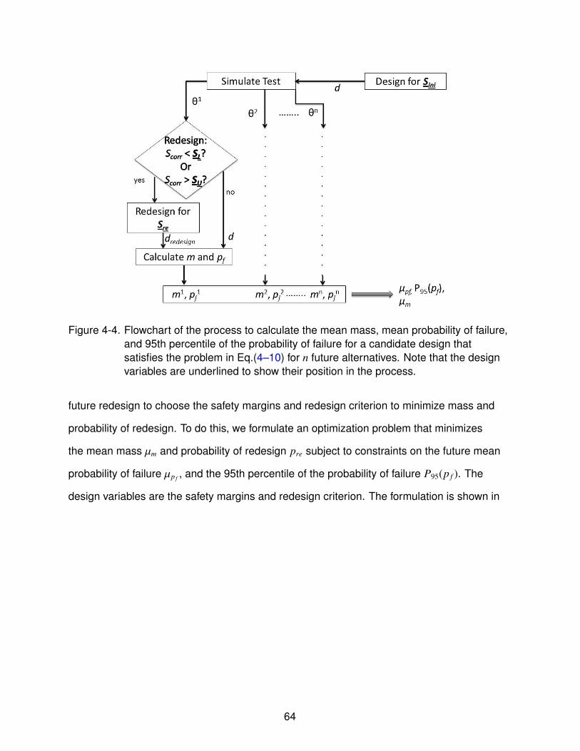
Figure 4-4. Flowchart of the process to calculate the mean mass, mean probability of failure,and 95th percentile of the probability of failure for a candidate design thatsatisfies the problem in Eq.(4–10) for n future alternatives. Note that the designvariables are underlined to show their position in the process.

future redesign to choose the safety margins and redesign criterion to minimize mass and

probability of redesign. To do this, we formulate an optimization problem that minimizes

the mean mass µm and probability of redesign pre subject to constraints on the future mean

probability of failure µp f , and the 95th percentile of the probability of failure P95(p f ). The

design variables are the safety margins and redesign criterion. The formulation is shown in

64

Eq.(4–10).

minS ini,S L,S U ,S re

µm, pre

subject to (µp f )Be f oreRedesign ≤ 0.1%

(P95(p f ))Be f oreRedesign ≤ 0.5%

(µp f )A f terRedesign ≤ 0.01%

(P95(p f ))A f terRedesign ≤ 0.05%

35 ≤ S ini, S re ≤ 65

S ini − 35 ≤ S L ≤ S ini

S ini ≤ S U ≤ S ini + 35

1.24mm ≤ tw ≤ 1.77mm

4.94mm ≤ tB ≤ 7.06mm

49.9mm ≤ dS ≤ 71.3mm

(4–10)

The constraints on S ini and S re restrict the two values to be within the window of 35 to

65 K, and they are not constrained to have equal values. The lower limit is intended to reflect

a regulatory mandate, but, just in case, bounds on the before redesign probability of failure

are present to prevent designs that are largely unsafe before redesign. The constraints

on S L and S U restrict the acceptable values of the safety margin after correction to within

35 K of S ini. Note that in this chapter the design and redesign policy is optimized on the

basis of a single panel. If an optimization like that is carried out in practice, we assume that

compromise values will be used based on similar optimization for several cases.

For this problem, the computational and experimental errors were distributed as

described in Table 4-3. Given these distributions, the correction factor θ ranged from 0.85

to 1.15. The distributions of the variables with uncertainty due to variability are provided in

Appendix D.

To reduce the computational cost of simulating a future test, surrogates of the mass and

reliability index were developed. The reliability index β is related to the probability of failure

65

Table 4-3. Bounds of computational and experimental errorsError Distribution Boundsec Uniform ±0.12ex Uniform ±0.03

by p f = Φ(−β), where Φ is the standard normal cumulative density function. For example,

for a probability of failure of 0.1%, the reliability index is 3.72. The development of these

surrogates is described in Appendix C.

The problem in Eq.(4–10) was solved by forming a cloud of 10,000 points using Latin

Hypercube sampling of the design variables S ini, S L, S U , and S re. For each set of design

variables, 10,000 alternative futures were sampled to obtain the distributions of the mass

and probability of failure, and the probability of redesign. The set of points that satisfied the

constraints on the probability of failure was found, and, from this set of feasible points, we

formed the Pareto front for minimum probability of redesign and mean mass after redesign.

4.7.2 Results

As a point of comparison, we first found the optimum design for minimum mass that

satisfied the “before redesign” constraints on the probability of failure. Since redesign was

not performed, the only value of interest is S ini. The minimum value of S ini = 48.9 K which

satisfied the probability constraints of a mean of 0.1% and 95th percentile of 0.5% led to

a mass of 24.7 kg/m2. In addition, we found the minimum S ini design that satisfied the

“after redesign” probability of failure constraints without actually performing redesign (i.e.,

the minimum S ini that satisfied µp f ≤ 0.01% and P95(p f ) ≤ 0.05% without any redesign).

In this case, the minimum S ini was 62.5 K for a mass of 25.3 kg/m3 for µp f = 0.01% and

P95(p f ) = 0.05%. Plots of the probability density of the safety margin after correction (i.e.,

S corr = Tallow − Tcalc,corr) for the S ini = 48.9 K and S ini = 62.5 K cases are shown in Fig. 4-5.

Figure 4-5 shows the distribution of the corrected safety margins with the two values

of S ini. The figure also shows the value of S needed to achieve the desired probabilities of

failure (S ini = 29.7 K for µp f = 0.1% in Fig. 4-5(a) and S ini = 41.3 K for µp f = 0.01% in Fig.

4-5(b)) in the absence of epistemic uncertainty. We observed that 79% of S corr values were

66

(a) S ini = 48.9K (b) S ini = 62.5K

Figure 4-5. Probability density function of the safety margin after correction for (a)S ini = 48.9K which also displays the S ini required in the absence of epistemicuncertainty for a mass of 23.9kg/m2 and (b) S ini = 62.5K which also displays theS ini required in the absence of epistemic uncertainty for a mass of 24.3kg/m2

greater than 29.7 K for S ini = 48.9 K and 84% greater than 62.5 K for for S ini = 41.3 K. This

was because the mean probability of failure was influenced disproportionally by a few large

values as the median probability of failure before redesign was 7.3e-4% for S ini = 48.9 K and

3.2e-6% for S ini = 62.5 K. The figure caption also notes that the mass required to achieve

the desired probability of failure in the absence of epistemic uncertainties was 23.9kg/m2

for 0.1% and 24.3kg/m2 for 0.01%. With the epistemic uncertainty, we required 25.3kg/m2

to compensate for the computational error, and this 1 kg/m2 or 4% penalty was what can be

reduced by more accurate computation or tests.

Allowing redesign, the Pareto front for minimum probability of redesign and mean

mass after redesign is displayed in Fig. 4-6 that satisfies the constraints of the problem in

Eq.(4–10). We observed reductions in mean mass with increasing probabilities of redesign.

The mean mass values after redesign at these points were less than the minimum mass

of 25.3 kg/m3 obtained when redesign was not allowed. At 40% probability of redesign,

the mean mass was even less than 24.7 kg/m3, the mass of the optimum design that

67

satisfied the relaxed “before redesign” constraints on probability of failure (µp f ≤ 0.1% and

P95(p f ) ≤ 0.5%).

Figure 4-6. Pareto front for minimum probability of redesign and mean mass after redesign.Feasible points in the design space are shown, along with the before-redesignmass of the points on the Pareto front

The values of the safety margins for the designs on the Pareto front are displayed in Fig.

4-7. We observed that the initial safety margin S ini was nearly constant at approximately 63

K. The lower bound of the acceptable safety margin with correction S L remained between 28

to 32 K, for which the difference from S ini is near the upper bound of 35 K (i.e., the constraint

on the lower bound of S L is active or nearly active). This resulted in the small probability of

redesign of unconservative designs. In Fig. 4-8, which shows the percentage of the total

probability of redesign that is conservative and unconservative, we observed that this was

indeed the case, and that less than 5% of the total probability of redesign was attributed to

unconservative redesign for all points on the Pareto front.

For the upper bound on acceptable safety margin with correction S U , we observed

that the values were large (nearly 100 K) but gradually reduced to values near S ini at 65 K.

This led to the gradual increase in probability of conservative redesign as the probability

of unconservative redesign remained at low values. Thus, the probability of conservative

68

(a) Initial and redesign safety margins (b) Bounds of corrected safety margin

Figure 4-7. For Pareto front for minimum probability of redesign and mean mass afterredesign, (a) initial and redesign safety margins versus total probability ofredesign and (b) bounds of the acceptable corrected safety margins versus totalprobability of redesign

Figure 4-8. Percentage of conservative and unconservative redesigns of the points on thePareto front

redesign comprised the majority of the total probability of redesign for the designs on the

Pareto front. At the same time, we observed that the safety margin S re of the redesign

was set to values below S ini and at values less than the minimum value without tests and

redesign of 63.5 K. That is, after the test, the redesign has a smaller safety margin than

possible for the original design. This value is even less that the safety margin required to

satisfy the relaxed before redesign constraints of S ini = 48.9 K. The combined effect of

69

redesigning conservative designs for a reduced safety margin was a reduction in the mean

mass while satisfying more stringent constraints on the probability of failure.

The results show that the optimal choice safety margins and redesign criterion can be

chosen based on the probability of failure that accounts for future redesign. We observe

that companies can benefit by having designers consider conservative safety margins for

the initial design, which correspond to the safety margin required to satisfy the probabilistic

constraints. The redesign criterion should then mostly result in the redesign of overly

conservative designs to trim mass by allowing a smaller safety margin for redesign (because

of additional knowledge due to the test in the correction factor), with a few unsafe designs

redesigned for safety.

4.7.3 Unconservative Initial Design Approach

While the Pareto optimal designs showed that the initial design should be conservative

with redesign performed to trim mass, we examined the trade-off in probability of redesign

and mass when starting with an initially unconservative design (i.e., an initial design that

does not satisfy the constraints of p f ). In this approach, the designer uses a smaller

safety margin to achieve a minimal weight design, relying on the test and redesign to

correct any dangerous designs. In this problem, the initial safety margin was fixed at 48.9

K (corresponding to a mass of 24.7 kg/m2) and the remaining safety margins (S re, S L, and

S U) were the design variables. The same constraints as in Eq.(4–10) were used. Figure 4-9

displays the Pareto front found with the unconservative approach, and compares the result to

the previously found results that used a conservative-first approach found in Sec. 4.7.2.

It was observed that to meet the probability of failure requirements, the probability of

redesign was at least 27% for the unconservative approach with S ini = 48.9 K. That is, the

designer must accept at least a 27% probability of redesign, which would lead to a mean

mass of approximately 25.2 kg/m2. This value of the mass is only 0.4% smaller than the

initial mass required to satisfy the probability constraints without redesign with the initially

conservative design.

70

Figure 4-9. Pareto front showing the Pareto front found for the unconservative approach (withS ini = 48.9 K) in comparison to the Pareto front with the conservative approach(with S ini = 62.5 K)

.

Figure 4-10 displays the values of the design variables of the Pareto optimal solutions,

and Fig. 4-11 displays the breakdown of the total probability of redesign due to conservative

and unconservative designs. It was observed that redesign was primarily performed to

increase safety at the smallest probabilities of redesign (27%), increasing the redesign of

conservative designs with increasing probability of redesign.

The histogram of the mass for 10,000 alternative futures after redesign is displayed in

Fig. 4-12(a). The approximately 2% increase in the mean mass after redesign is attributed

to the large probabilities of failure associated with redesign of unconservative designs. A

breakdown of the alternative futures that resulted in the mean mass is shown in Table 4-4. It

was observed that the redesign of unconservative designs resulted in a increase of 8% in the

mean mass.

In contrast, the same mean mass of 25.2 kg/m2 after redesign can be achieved with the

conservative-first approach with a probability of redesign around 8%, and for a probability of

redesign of 27%, the mean mass is nearly 24.7 kg/m2. In this case, the reduction in mean

71

(a) Initial and redesign safety margins (b) Bounds of corrected safety margin

Figure 4-10. For Pareto front for minimum probability of redesign and mean mass afterredesign with the unconservative-first approach, (a) initial and redesign safetymargins versus total probability of redesign and (b) bounds of the acceptablecorrected safety margins versus total probability of redesign

Figure 4-11. Percentage of conservative and unconservative redesigns of the points on thePareto front with the unconservative-first approach

mass is due to large reductions in mass in the cases that required redesign of conservative

designs. The histogram of the mass for 10,000 alternative futures is shown in Fig. 4-12(b)

and the mass and probability of redesign is detailed in Table 4-4. It was observed that the

redesign of overly conservative designs resulted in a 10% reduction in the mean mass.

72

(a) Initially Unconservative (b) Initially Conservative

Figure 4-12. Histograms of mass after redesign for 10,000 alternative futures for (a) initiallyunconservative design with 27% probability of redesign and (b) initiallyconservative design with 8% probability of redesign.

Table 4-4. Breakdown of alternative futures for the unconservative initial design with 27%probability of redesign and conservative initial design with 8% probability ofredesign

Outcome pre (%) Mean Mass (kg/m2)Initially Unconservative

No redesign 73 24.7Unconservative 25.5 26.8Conservative 1.5 23.5Total 25.21

Initially ConservativeNo redesign 93.5 25.3Unconservative 2.1 25.8Conservative 4.4 22.7Total 25.21

1 Calculated as pnoredesignm0+(preµm)conservative+

(preµm)unconservative

Comparing this value along with the 8% increase in mass seen in the initially unconservative

case, we observed that the change in mass due to redesign is much larger than the 2%

difference in mass of the two initial designs. However, with the initially conservative design

most redesigns act to reduce the mass, whereas the mass is mostly increased in the initially

unconservative redesign cases. Therefore, the designer has a choice:

73

1. use a smaller initial safety margin for an initially small mass and accept a 27% proba-bility of redesign that will increase the mass, or

2. use a larger initial safety margin for an initially larger mass that can achieve less thanor equal to the same mass with probabilities of redesign greater than 8%.

If the test shows the component does not have to be redesigned, there would be a nearly 2%

mass penalty in using the conservative safety margin.

4.7.4 Discussion

Using the minimal safety margin for the initial design can be thought of as using safety

margins given by regulatory agencies, which provide minimum values of safety margins

and safety factors. For example, the Federal Aviation Administration has recommended

minimum design and test factors for structures on reusable launch vehicles [72]. In this work,

the values of S ini (and S re) of 35 K may be the minimum value imposed by an agency, and

the value of 48.9 K may be the current minimum value imposed by a company based on

history or experience. The results presented in the chapter show that a company may have

an incentive to impose their own safety margins, and set the design and redesign rules to

balance development costs. The results in Sec. 4.7.2 showed that probabilistic constraints

can be satisfied by first using a conservative safety margin and accepting a risk of increased

development cost through increased redesign to trim excess mass. This directly contrasts

the approach of using minimal safety margin values and redesigning based on the test result

to increase safety. Considering the possible future redesign and its cost allows the company

to make better decisions at the design stage.

4.8 Summary and Discussion on Possible Future Research Directions

In this chapter, we used the modeling of future redesign to provide a way of balancing

development costs (test and redesign costs) and performance (mass) by designing the

design and redesign rules. We observed that the presence of epistemic uncertainty led to

a mass penalty, which could be reduced by a test and redesign. Since deterministic design

employing safety margins and safety factors is common practice in industry, we showed

that safety margins and redesign criteria can be chosen using the probability of failure with

74

future redesign. A study on an integrated thermal protection system showed that a minimum

mass design that satisfied probabilistic constraints can be achieved by having an initially

conservative design and a redesign criterion such that redesign is mainly performed on

overly conservative designs to trim excess mass. In contrast, we examined the trade-off in

starting with an initially small safety margin, which may be a minimum value recommended

by a regulatory agency, and using the test and redesign to correct dangerous designs.

Therefore, in this example, a company would have an incentive to use conservative safety

margins at the initial design stage, while increasing performance by implementing a redesign

criterion aimed at discovering overly conservative designs. This also provides a balance

between probabilistic design and the more traditional deterministic approach.

Possible future research includes considering the uncertainty reduction methods that

often take place after a component is designed but before a component is tested. For

example, lower fidelity methods may be used to find a starting point for the initial design.

Before a design is tested, it may be better characterized through higher fidelity modeling or

optimization in a smaller design space about this design. Both the higher fidelity modeling

and re-optimization can reduce the uncertainty in the design before a test is even performed.

Therefore, a study that models these actions and considers the subsequent uncertainty

reduction would be useful in finding the optimal balance in design and development costs

and performance.

75

CHAPTER 5DYNAMIC DESIGN SPACE PARTITIONING FOR LOCATING MULTIPLE OPTIMA: AN

AGENT-INSPIRED APPROACH

In this chapter, we explore the use of design space partitioning to tackle optimization

problems in which each point is expensive to evaluate and there are multiple local optima.

The overarching goal of the method presented is to locate all local optima rather than

just the global one. Locating multiple designs provides insurance against discovering

that late in the design process a design is poor due to modeling errors or overlooked

objectives or constraints. The proposed strategy to locate multiple candidate designs

dynamically partitions the search space among several “agents” that approximate their

sub-region landscape using surrogates. Agents coordinate by exchanging points to form

an approximation of the objective function or constraints in the sub-region and by modifying

the boundaries of their sub-regions. Through a self-organized process of creation and

deletion, agents adapt the partition as to exploit potential local optima and explore unknown

regions. This idea is demonstrated on a six-dimensional analytical function, and a practical

engineering example, the design of an integrated thermal protection system.

As part of a history on this research, the idea of working in partitioned designs spaces

was born out of an idea to decompose the problem among several agents, which act to

solve their own sub-problems and coordinate to solve the global problem. Combined with

the idea of solving these sub-problems cheaply, we then turned to the use of surrogates to

approximate expensive objective functions or constraints. Thus, we developed a method-

ology, presented in this chapter, in which an agent uses its own local surrogate to solve

the sub-problem in its sub-region. The goal was to limit the amount of information shared

between the agents, where each agent would find the best solution in its region. Later on, as

presented in the next chapter, we explored the effectiveness of using local surrogates rather

than global surrogates and also the use of partitions rather than starting optimization runs

from different points of the design space.

76

5.1 Motivation and Background on Locating Multiple Optima

Many contemporary applications can be modeled as distributed optimization problems

(ambient intelligence, machine-to-machine infrastructures, collective robotics, complex

product design, etc.). Optimization processes iteratively choose new points in the search

space and evaluate their performances until a solution is found. However, a practical and

common difficulty in optimization problems is that the evaluations of new points require ex-

pensive computations. For instance, if one wants to compute a property of a complex object

(e.g. large deflections of an aircraft wing under some loading), a high fidelity computation

(e.g. finite element analysis) may be required. Therefore, many researchers in the field of

optimization have focused on the development of optimization methods adapted to expensive

computations. The main ideas underlying such methods are often the use of surrogates,

problem decomposition, and parallel computation. The use of surrogates to replace ex-

pensive computations and experiments in optimization has been well documented [40–43].

Moreover, in optimization, a common way to decompose problems is to partition the search

space [73, 74]. Furthermore, to take advantage of parallel computing, many have proposed

strategies for using multiple surrogates in optimization [9–12]. The goal of most of these

algorithms is to locate the global optimum, while trying to minimize the number of calls to

the expensive functions. Like these algorithms, we try to reduce the number the number of

calls to the expensive functions, but our main goal is to locate multiple optima as multiple

candidate designs. For real-world problems, the ability to locate many optima in a limited

computational budget is desirable as the global optimum may be too expensive to find, and

because it provides the user with a diverse set of acceptable solutions as insurance against

late formulation changes (e.g., new constraints) in the design process.

Besides the aforementioned techniques for distributing the solving process, multi-

agent optimization is an active research field proposing solutions for distinct agents to

cooperatively find solutions to distributed problems [75]. They mainly rely on the distribution

(and decomposition) of the formulation of the problem. Generally, the optimization framework

77

consists of distributing variables and constraints among several agents that cooperate to set

values to variables that optimize a given cost function, like in the DCOP model [14]. Another

approach is to decompose or transform problems into dual forms that can be solved by

separate agents [15] (for problems with specific properties, such as linearity).

Here, we describe a multi-agent method in which the search space is dynamically

partitioned (and not the problem formulation) into sub-regions in which each agent evolves

and performs a surrogate-based continuous optimization. The novelty of this approach

comes from the joint use of (i) surrogate-based optimization techniques for expensive

computation and (ii) self-organization techniques for partitioning the search space and

finding all the local optima. Coordination between agents, through exchange of points and

self-organized evolution of the sub-region boundaries allows the agents to stabilize around

local optima. Like some nature-inspired niching methods [76, 77], such as particle swarm

[78–80] and genetic algorithms [81, 82], or clustering global optimization algorithms [83], our

goal is to locate multiple optima, but unlike these algorithms, our approach aims to sparingly

call the true objective function and constraints. Our multi-agent approach further (i) uses

the creation of agents for exploring the search space and, (ii) merges or deletes agents to

increase efficiency.

Additionally, the use of surrogates combined with partitioning of the design space allows

us to take advantage of local search methods by aiming to optimize using the surrogate

predictions rather than the true functions. Here, we propose a methodology that aims to

first exploit the surrogate prediction (i.e., by seeking first to minimize the function) and only

explore when no points that lead to further improvements can be found. Thus, in this method

we do not aim to explicitly balance exploitation versus exploration iterations as with most

global optimization algorithms, but instead primarily exploit, and explore through design

space partitioning and the occasional addition of space filling points.

In the following section, we discuss more deeply the motivation for multiple candidate

designs. Next, we provide some background on surrogate-based optimization. In Sec. 5.4,

78

we describe the autonomous agents that perform the cooperative optimization process.

In Sec. 5.5, we present the methods of space partitioning and point allocation that are

intended to distribute local optima among the partitions while maximizing the accuracy of

the surrogate in a self-organized way – through agent creation and deletion. In Sec. 5.6 a

six-dimensional problem is tackled using our multi-agent optimizer, and in Sec. 5.7 a practical

engineering example, the design of an integrated thermal protection system, is presented.

5.2 Motivation for Multiple Candidate Designs

In optimization courses, we often tell students that defining an optimization problem

properly is the most important step for obtaining a good design. However, even experienced

hands often overlook important objective functions and constraints. There are also epistemic

uncertainties, such as modeling errors, in the objective functions and constraints definitions

that will typically perturb their relative values throughout the design space. In one case, Na-

gendra et al. [81] used a genetic algorithm to find several structural designs with comparable

weight and identical load carrying capacity. However, when three of these designs were

built and tested, their load carrying capacity was found to differ by 10%. For such reasons,

alternative local optima may be better practical solutions to a given optimization problem than

a single idealized global optimum. As advances in computer power have made it possible to

move from settling on local optima to finding the global optimum, when designing engineer-

ing systems. This usually requires search in multiple regions of design space, expending

most of the computation needed to define multiple alternate designs. Thus, focusing solely

on locating the best design may be wasteful.

In engineering design, the simulated behavior of objective functions and constraints

usually has modeling error, or epistemic uncertainty, due to the inability to perfectly model

phenomena. Modeling errors can degrade local optima or even cause them to disappear.

Let us now turn to a practical engineering design example to demonstrate the presence,

diversity, and fragility of candidate designs. Large portions of the exterior surface of many

space vehicles are devoted to providing protection from the severe aerodynamic heating

79

experienced during ascent and atmospheric reentry. A proposed integrated thermal pro-

tection system (ITPS) provides structural load bearing function in addition to its insulation

function and in doing so provides a chance to reduce launch weight. Figure 5-1 displays the

corrugated-core sandwich panel concept of an ITPS, which consists of top and bottom face

sheets, webs, and insulation foam between the webs and face sheets.

Figure 5-1. Integrated thermal protection system provides both insulation and load carryingcapacity, and consequently can lead to alternative optima of similar mass butdifferent way of addressing the thermal and structural requirements.

The thermal and structural requirements often conflict due to the nature of the mecha-

nisms that protect against the failure in the different modes. For example, thin webs prevent

the flow of heat to the bottom face but are more susceptible to buckling and strength failure.

A reduction in foam thickness (panel depth) improves resistance against buckling of the

webs but increases heat flow. A thick bottom face sheet acts as a heat sink and reduces the

temperature at the bottom face but increases stress in the web.

These conflicts may be resolved by candidate designs in different ways. Figure 5-2

displays the infeasible and feasible regions with constraints on the temperature of the bottom

face sheet and stress in the web for the three-dimensional example, in which the web, bottom

face, and foam thicknesses were the design variables.

Three islands of feasibility are observed, in which the design is driven to protect against

different failure modes. The two minimum mass designs are in Regions 1 and 2. In Region

1, the failure is primarily from stress, because the webs are thin. This is compensated by

80

Figure 5-2. Feasible regions 1-3 and infeasible regions (left) and mass objective functionrepresented by color (right). The two competitive optima in Regions 1 and 2 relyon different concepts. In Region 1 the thermal function is satisfied by a thickbottom face sheet acting as heat sink, while in Region 2 it is satisfied by thickinsulation.

reducing the length of the web by reducing the foam thickness, and to compensate for

the increase heat flow, the bottom face sheet is increased to provide a larger heat sink. In

Region 2, both failure modes are present, so that the insulation is thicker to prevent thermal

failure and the bottom face is thinner to reduce stress in the web. With both feasible regions

being rather narrow, modeling errors can easily wipe out one of these regions, so that having

both designs provides valuable insurance. Furthermore, even if modeling errors do not wipe

out Region 2 but only narrow it, this can result in substantial increase in mass, while Region

1 is more robust.

This example demonstrates the benefit of multiple candidate designs due to the

fragility designs from errors. In the following sections, the dynamic design space partitioning

algorithm is described, and a six dimensional analytical example is presented before

returning to the ITPS example in Sec. 5.7.

81

5.3 Surrogate-Based Optimization

A surrogate is a mathematical function that (i) approximates outputs of a studied model

(e.g. the mass or the strength or the range of an aircraft as a function of its dimensions),

(ii) is of low computation cost and (iii) aims at predicting new outputs [84]. The set of initial

candidate solutions, or points, used to fit the surrogate is called the design of experiments

(DOE). Known examples of surrogates are polynomial response surface, splines, neural

networks or kriging.

Let us consider the general formulation of a constrained optimization problem,

minimizex∈S⊂ℜn

f (x)

subject to g(x) ≤ 0(5–1)

In surrogate-based optimization, a surrogate is built from a DOE, denoted by X that consists

of sets of the design variables x. For the design of experiments, there are the calculated

values of the objective function f and constraints g that are associated with the DOE, which

we denote as F and G, respectively. We will refer to X and its associated values of F and G

as a database.

The database is used to construct the surrogate approximation of the objective function

f and the approximation of the constraint g. We can approximate the problem in Eq.(5–1)

using the surrogates and formulate the problem as


f (x)


The solution to this approximate problem is denoted x∗.

Surrogate-based optimization calls for more iterations to find the true optimum, and

is therefore dependent on some iteration time t. That is, after the optimum of the problem

in Eq.(5–2) is found, the true values f (x∗) and g(x∗) are calculated and included in the

DOE along with x∗. At the next iteration, the surrogate is updated, and the optimization is

82

performed again. Therefore, we denote the DOE at a time t as Xt and the associated set of

objective function values and constraint values as Ft and Gt, respectively. The surrogate-

based optimization procedure is summarized in Algorithm 2 (which also refers to a global

optimization procedure in Algorithm 3).

Algorithm 2 Overall surrogate-based optimization1: t = 1 (initial state)2: while t ≤ tmax do3: Build surrogates f and g from (Xt,Ft,Gt)4: Optimization to find x∗ (see Algorithm 3)5: Calculate f (x∗) and g(x∗)6: Update database (Xt,Ft,Gt) ∪ (x∗, f (x∗), g(x∗))7: t = t + 18: end while

Algorithm 3 Constrained optimization procedure

1: Input: f , g, Xt,L2: Output: x∗

3: x∗ ← argminx∈L

f (x) subject to g(x) ≤ 0

4: if x∗ is near Xt or out of the search domain L then5: x∗ ← argmax

x∈Sdistance(Xt)

6: end if

5.4 Agent Optimization Behavior

As stated in the introduction, our approach consists in splitting the space in sub-regions

and assigning agents to each of these sub-regions as presented in Fig. 5-3. Therefore,

Algorithm 6 can be thought of as the procedure followed by a single agent to find one point,

that will be repeating until termination. However, in the multi-agent approach we describe

here, each agent is restricted to only a sub-region of the design space, i.e., S is replaced

by a part of S. The rationale behind this idea is that each agent has an easier optimization

subproblem to solve because it searches a smaller space, which we denote as Pi for the ith

agent, and considers a simpler function. Each agent must consider only the points in its sub-

region, which are available in its internal database (Xt,Ft,Gt)i. The sub-region of an agent

is defined by the position of its center c. A point in the space belongs to the sub-region with

83

the nearest center, where the distance is the Euclidean distance. This creates sub-regions

that are Voronoi cells [85]. The choice of where to place the center is discussed in the next

section. Figure 5-3 illustrates the partition of a two-dimensional space into four sub-regions

for four agents, which requires four centers. In this example, we place the centers randomly.

space partitions will be discussed in Section 5.5.

Figure 5-3. Multi-agent System overview: agents perform surrogate-based optimization indifferent sub-regions of the partitioned search space based on personalsurrogates (dashed l.) and exchange points with their direct neighbors (dotted l.)

The procedure of a single agent is given in Algorithm 4. Assuming that sub-regions are

defined, each agent fits several surrogates it knows (as many different ways to approximate)

and chooses the one that maximizes the accuracy in its sub-region (line 5-9). To avoid

ill-conditioning, if more points are needed than are available to an agent, the agent asks

neighboring agents for points. The neighboring agents then communicate the information

associated with these points (lines 6–8). We define the best surrogate as the one with the

minimum cross-validation error, the partial prediction error sum of squares PRES S RMS . This

is found by leaving out a point, refitting the surrogate, and measuring the error at that point.

The operation is repeated for p points in the agent’s sub-region (disregarding any points

received from other agents) to form a vector of the cross-validation errors eXV . The value of

84

PRES S RMS is then calculated by

PRES S RMS =

√1p

eTXVeXV (5–3)

Algorithm 4 Agent i optimization in its sub-region.1: t = 1 (initial state)2: while t ≤ tmax do3: Update Pi = {x ∈ S s.t.||x − ci||2 ≤ ||x − c j||2 , j , i}4: Update internal database from the new space partition5: Build surrogates f and g from (Xt,Ft,Gt)i

6: if Not sufficient number of points in internal database to build a surrogate then7: Get points from other agents closest to ci

8: Build surrogates9: end if

10: Choose best surrogate based on partial PRES S RMS error11: Optimization to find x∗ [with Algorithm 3 ( f , g,Xt,Pi)]12: Calculate f (x∗) and g(x∗)13: (Xt+1,Ft+1,Gt+1)i ← (Xt,Ft,Gt)i ∪ (x∗, f (x∗), g(x∗))14: Update center ci (see Section 5.5.1)15: Check for merge, split or create (see Section 5.5.2)16: t = t + 117: end while

Once the agents have chosen surrogates (line 10), the optimization is performed to

solve the problem in Eq.(5–2) inside the sub-region (line 11). If the optimizer gives an

infeasible point (i.e., the point does not satisfy the constraint in Eq.(5–2) or is out of the sub-

region) or repeats an existing point, the agent then explores to find an alternate point in the

sub-region. To explore, the agent adds a point to the database that maximizes the minimum

distance from the points already in its internal database (see Algorithm 3). The true values f

and g of the iterate are then calculated (line 12), and (x∗, f (x∗), g(x∗)) is added to the internal

database (lines 12–13).

5.5 Dynamic Design Space Partitioning

The previous section expounds the cooperative optimization process performed by

agents in a pre-partitioned space. The goal of this method is to have each agent locate a

single optimum, such that the partitioning strongly depends on the topology of the space.

85

Therefore, as a part of the cooperative optimization process, we propose a self-organizing

mechanism to dynamically partition the space which adapts to the search space. By self-

organizing, we mean that agents (and therefore sub-regions) will be created and deleted

depending on the cooperative optimization process. Agents will split when points are

clustered inside a single region (creation), and will be merged when local optima converge

(deletion).

5.5.1 Moving the Sub-regions’ Centers

The method of space partitioning we propose focuses on moving the sub-regions’

centers to different local optima. As a result, each agent can choose a surrogate that is

accurate around the local optimum, and the agent can also explore the sub-region around

the local optimum. At the beginning of the process, only one agent exists and is assigned to

the whole search space. Then it begins optimization by choosing a surrogate, fitting it and

optimizing on this surrogate. As a result the agent computes a new point x∗t−1. Then, the

center of the sub-region is moved to the “best” point in the sub-region in terms of feasibility

and objective function value (line 14). This is done by comparing the center at the last

iteration ct−1 to the last point added by the agent x∗t−1. The center is moved to the last point

added by the agent if it is better than the current center. Otherwise, the center remains at the

previous center. For convenience, in comparing two points xm and xn, we use the notation

xm ≻ xn to represent xm “is better than” xn. For two centers, instead of points x we would

consider the centers c. The conditions to determine the better of two points are given in

Algorithm 5.

5.5.2 Merge, Split and Create Sub-regions

Once an agent has added a new point in its database (line 13) and moved its center

to the best point (line 14), it will check whether to split, or to merge with other ones (line

15). Merging agents (and their sub-regions) prevents agents from crowding the same area,

allowing one agent to capture the behavior in a region. Splitting an agent is a way to explore

the space as it refines the partitioning of the space in addition to the search that each agent

86

Algorithm 5 Algorithm to determining if, for two points xm and xn, xm “is better than” xn

(xm ≻ xn) and vice versa. Note that for the algorithm below, the time (superscript t) is omittedas the algorithm is valid for the comparison of any two points at any time.

1: Given f (xm), f (xn),max(g(xm)),max(g(xn))2: if max(g(xm)) ≤ 0 & max(g(xn)) ≤ 0 then3: // both points are feasible4: if f (xm) ≤ f (xn) then5: xm ≻ xn

6: else7: xn ≻ xm

8: end if9: else if max(g(xm)) ≤ 0 & max(g(xn)) > 0 then

10: // only xm is feasible11: xm ≻ xn

12: else if max(g(xm)) > 0 & max(g(xn)) ≤ 0 then13: // only xn is feasible14: xn ≻ xm

15: else if max(g(xm)) > 0 & max(g(xn)) > 0 then16: // both are infeasible17: if max(g(xm)) ≤ max(g(xn)) then18: // maximum constraint violation of xm is less thanxn

19: xm ≻ xn

20: else21: xn ≻ xm

22: end if23: end if

can perform in its sub-region. Split and merge occurs at the end of each iteration (line 15):

agents are first merged (if necessary), the points belonging to the merged agent(s) are

distributed to the remaining agents based on distance from the center of the remaining

agents’ sub-regions, and then each remaining agents examines to determine whether to split

or not.

5.5.2.1 Merge converging agents

Agents are merged (deleted) if the centers of the agents’ sub-regions are too close as

measured by the Euclidean distance between the centers. We measure the minimum Eu-

clidean distance between two centers as a percentage of the maximum possible Euclidean

distance between points in the design space. When examining the agents, the agent with the

87

center with the lowest performance is deleted. For example, for agents 1 and 2, if c1 ≻ c2,

agent 2 is deleted. Before deletion, the deleted agent distributes its internal database points

to closest neighbors.

5.5.2.2 Split clustered sub-regions

It is desirable to create an agent if it is found that points are clustered in two separate

areas of a single agent’s sub-region, as illustrated in Fig.5-4(a). Such a situation can occur if

there are two optima in a subregion.

.........................

Potential clusters

.

Present bestsolution &

Agent i’s center

.

(a) Potential clusters within a sub-region

.......................

Centers from k-means

.


Agent i’s center

...c1..

c2

(b) Clusters from k-means

..................................

New agent j’s center

.


Agent i’s center

... c2

(c) Final clusters after moving centers topresent best solution and nearest datapoint

Figure 5-4. Illustration of process used to create an agent j given points in a single agent i’ssub-region.

Agents are created by using k-means clustering [86] for two clusters (k = 2) given the

points in the sub-region, where the initial guesses of the centers are the present best solution

(the current center) and the mean of the dataset. Since k-means clustering gives centers

that are not current data points as illustrated in Fig.5-4(b), we move the centers to available

data points to avoid more calls to evaluate the expensive functions. This is done by first

88

measuring the distance of the centers from k-means to the present best solution, and moving

the closest center to the present best solution, as we want to preserve this solution. For the

other center, we measure the distance of the current data points to the other center, and

make the closest data point the other center. The final clustering is illustrated in Fig.5-4(c).

The result is a new agent with a center at an already existing data point, where the creating

agent retains its center at its present best solution.

This final clustering is validated using the mean silhouette value of the points in the

sub-region. The silhouette, introduced by Rousseeuw [87], is used to validate the number

of clusters, by providing a measure of the within-cluster tightness and separation from other

clusters for each data point i for a set of points. The silhouette value for each point is given

as

s(i) =b(i) − a(i)

max{a(i), b(i)} (5–4)

where ai is the average distance between point i and all other points in the cluster to which

point i belongs, and bi is the minimum of the average distances between point i and the

points in the other clusters. The values of si range from -1 to 1. For si near zero, the point

could be assigned to another cluster. If si is near -1, the point is misclassified, and, if all

values are close to 1, the data set is well-clustered. The average silhouette of the data points

is often used to characterize a clustering. In this work, we accept the clustering if all si are

greater than 0 and the average value of the silhouette is greater than some value.

5.5.2.3 Create new agents

The agents may reach a point where there is no improvement made by the overall

system in several iterations (i.e., the centers of all agents have remained at the same

points). For example, this can occur when each agent has located the best point in its

sub-region, the area around each best point is populated by points, each agent is driven

to explore for several iterations, and no other potential local optima are located. This can

also occur at early iterations in which the surrogates are not well-trained in the sub-region.

In order to improve exploration, a new agent is created in the design space when there is

89

no improvement for n iterations (i.e., the centers of the sub-regions have not moved for n

iterations). We call this parameter the stagnation threshold. To create a new agent, a new

center is created at an already existing data point that maximizes the minimum distance

from the already existing centers, thus forming a new agent. The design space is then

repartitioned.

5.6 Six-Dimensional Analytical Example

In this section, we examine the six-dimensional Hartman function (Hartman 6) that is

often used to test global optimization algorithms.

minimizex

fhart(x) = −q∑

i=1

aiexp

− m∑j=1

bi j(x j − di j)2

subject to 0 ≤ x j ≤ 1, j = 1, 2, . . . ,m = 6

(5–5)

In this instance of Hartman 6, q = 4 and a =[1.0 1.2 3.0 3.2

]where

B =

10.0 3.0 17.0 3.5 1.7 8.0

0.05 10.0 17.0 0.1 8.0 14.0

3.0 3.5 1.7 10.0 17.0 8.0

17.0 8.0 0.05 10.0 1.0 14.0

D =

0.1312 0.1696 0.5569 0.0124 0.8283 0.5886

0.2329 0.4135 0.8307 0.3736 0.1004 0.9991

0.2348 0.1451 0.3522 0.2883 0.3047 0.3047

0.4047 0.8828 0.8732 0.5743 0.1091 0.0381

As we wish to locate multiple optima, we modified Hartman 6 to contain 4 distinct local

optima by “drilling” two additional Gaussian holes at two locations to form two local optima,

in addition to the global optimum and one local optimum provided in the literature [39]. The

modified Hartman 6 function is

f (x) = fhart(x) − 0.52ϕ1(x) − 0.18ϕ2(x) (5–6)

90

where the mean and standard deviation associated with ϕ1 and µ1 =

[0.66 0.07 0.27 0.95 0.48 0.13

]and σ = 0.3 (all directions), respectively. The mean and standard deviation associated with

ϕ2 and µ2 =

[0.87 0.52 0.91 0.04 0.95 0.55

]and σ2 = 0.25 (all directions), respectively.

The optima are displayed in Table 5-1. To obtain an approximate measure of the size of the

basins of attraction that contain the optima, we measured the percentage of local optimiza-

tion runs that converged to each optimum. To do this, twenty-thousand points were sampled

using Latin Hypercube sampling and a local optimization was performed starting at each one

of these points using a SQP algorithm.

Table 5-1. Modified Hartman6 optima and the percentage of runs that found each optimumwith multiple starts and a SQP optimizer

Optimum f x percentage of runsGlobal -3.33 (0.20 0.15 0.48 0.28 0.31 0.66) 50Local 1 -3.21 (0.40 0.88 0.79 0.57 0.16 0.04) 21Local 2 -3.00 (0.87 0.52 0.91 0.04 0.95 0.55) 9Local 3 -2.90 (0.64 0.07 0.27 0.95 0.48 0.13) 20

The percentage of starts that converged to an optimum is also a measure of the volume

of its basin of attraction in comparison to other basins. Since Local 2 has the smallest

percentage of runs, it was expected that it would be the most difficult optimum to locate by

the agents. Note, however, that in six-dimensional space a ratio of 9%50% in volume would be

produced by a ratio of 0.75 in characteristic dimension.

5.6.1 Experimental Setup

Since there are no nonlinear constraints, only the objective function is approximated by

surrogates.. The three possible surrogates, which are kriging surrogates with different trend

functions, are described in Table 5-2. From this set, each agent chose the best surrogate

based on PRES S RMS . The set of surrogates and the minimum number of points used to fit

each surrogate are provided in Table 5-2. If the minimum number of points are not available,

points are borrowed from neighboring sub-regions in the order of increasing distance to the

agent center, and, if the requirement is still not met, then all available points are used.

91

Table 5-2. Surrogates considered in this studyID Description minimum # of pts for fit1 Kriging (quadratic trend)

1.5 * # coefficients for quadratic response surface2 Kriging (linear trend)3 Kriging (constant trend)

The parameters in Table 5-3 were used for all results. These parameters include

maximum number of agents (e.g., the maximum number of computing nodes available),

parameters that dictate how close points and centers can be, and parameters that define

if a new agent should be created. Since we are simulating expensive function evaluations,

we also fixed a computational budget to 400 function evaluations. Beyond this number, the

system stops: this is our only termination criterion. Finally, we start the multi-agent system

with a single agent able to split and merge with time.

Table 5-3. Multi-Agent Parameters for modified Hartman 6Parameter ValueMax # of function evaluations 400Max # of agents 8Initial/Min # of agents 1Min distance between agent centers 10% of max possible distance in

spaceMinimum distance between points 1e-3 (absolute for each dimension)Min average silhouette 0.25Min # of points in each agent after creation 4Stagnation threshold 3

The success and efficiency of the multi-agent approach is compared to a single agent

system which performs a classical surrogate-based optimization procedure as described

in Algorithm 6. However, this single agent is unable to perform dynamic partitioning and

optimizes over the whole space. This single agent has also a computation budget of 400

calls to the expensive function. The single agent configuration is a standard to which we

compare our multi-agent optimizer.

In each case, (multi- or single agent), as to evaluate the capability of the algorithms

to explore the search space, we also ran several experiments for different initial DOE sizes

92

(351 , 56, and 100) that still account for the number of function evaluations. Therefore, for a

larger initial DOE, the system executes fewer steps. For each of the cases that were studied,

the results shown are the median of 50 repetitions (i.e, 50 different initial DOEs). The local

optimization problems were solved with a sequential quadratic programming (SQP) algorithm

[88]. DOEs are obtained using Latin Hypercube sampling and the maximin criterion for five

iterations.

5.6.2 Successes to Locate Optima

For 50 repetitions, the percentage of repetitions that successfully located a solution a

1% distance from the optimum with a single agent and a multi-agent system is shown in Fig.

5-5. This distance is the Euclidean distance normalized by the maximum possible distance

between points in the design space (here,√

6). It was observed that the single agent had

fewer successes with an equivalent number of function evaluations compared to the multi-

agent case. In both the single and multi-agent cases, Local 2 was the optimum that was the

most difficult to locate with less than 10 successes with a single agent and 32 successes

with a multi-agent system. Based on the small percentage of runs that located Local 2 with

multiple starts and the true function values with the SQP optimizer (c.f. Table 5-1), this was

not unexpected.

5.6.3 Agent Efficiency and Dynamics

The median objective function value of the solution closest to each optimum is shown

in Fig. 5-6. For the global optimum and Local 1, it was observed that the efficiency is nearly

equal in the single and multi-agent cases. It was also observed that the smaller DOEs

required fewer function evaluations to find these optima. For Local 2 and Local 3, the multi-

agent system has a clear advantage in finding solutions with the objective function near the

1 This does not satisfy the minimum required number of points for the fit, so all points areused (a single surrogate spans the entire design space) until a sufficient number of pointsare obtained.

93

Figure 5-5. For the modified Hartman 6 example, the percentage of repetitions that located asolution within 1% distance from each optimum.

true optimum value. While it is clear for the global optimum and Local 1 that smaller DOEs

are more efficient, there is no clear relationship between DOE size and efficiency (consider

Local 2). Recall that Local 2 was expected to be the most difficult optimum to find judging by

the small percentage of runs of multiple starts with the SQP optimizer that were successful.

These results confirm that exploration is required to locate Local 2, and the multi-agent

system, in which exploration is an inherent feature, is more capable of finding this optimum.

Exploration by the multi-agent system was measured by the percentage of calls to the

true objective function in which exploitation or exploration occurred as shown in Fig. 5-7.

We define an exploitation call as when the agent adds a point that minimizes the objective

function. Note that we constrained the minimum distance a new point should be from an

already existing data point so that multiple local optima could be located. Exploration is when

a random point is added by an agent. Exploration generally occurs when exploitation has

failed, meaning all starts in the sub-region resulted in points that were not far enough from

existing data points or were outside of the sub-region.

94

Figure 5-6. Median objective function value of solution closest to each optimum with numberof function evaluations. The single agent case is denoted by “S” and themulti-agent case by “M”, with the initial DOE size represented by the number.

Figure 5-7. For the modified Hartman 6 example, the percentage of points that were addedin exploitation or exploration.

We observed that the multi-agent case mostly performed exploitation with a few

explorations, whereas the single agent performed exploration only 1% of the time. This

could be due to the single agent seeking to tune around the global optimum and Local 1,

which it locates with the fewest function evaluations. The number of times in which the an

95

agent puts point to tune around the optimum can be reduced by increasing the minimum

distance between points. In addition, it was observed that the single agent was slowly adding

exploitation points in the vicinity of Local 3 as shown in Fig. 5-6.

Figure 5-8 shows the median number of agents. While up to 8 agents could be created,

it was observed that the median number of agents stabilized around 4, the number of local

optima. This is because once all the local optima are located, new agents are created but

are soon deleted as they converge to the basins of attraction of the already found optima.

Figure 5-8. For a multi-agent system, the median number of agents

The accuracy of the surrogates was measured by the partial PRES S RMS and the error

at 1000 test points by the erms. PRES S RMS is a leave-one-out cross-validation error. In the

single agent case the calculation of PRESS is straightforward, but for the multi-agent case it

is taken by calculating PRES S RMS in each sub-region and taking the mean of the values. The

values of PRES S RMS and eRMS are displayed in Fig. 5-9. The PRES S RMS indicated that the

error was decreasing for both the single and multi-agent cases, with the single agent case

slightly more accurate. However, the eRMS provided a more global indication of the accuracy

of the surrogate and showed that the approximation made by the multiple agents improved

with function evaluations more than the approximation of the single agent did. This is due

to the single agent putting many points near the global optimum and Local 1, making the

surrogate accurate in these locations but less accurate globally. The slow location of Local 3

96

by the single agent can also be partially explained by the poor accuracy of the single agent’s

surrogate.

(a) PRES S (b) erms

Figure 5-9. For the modified Hartman 6 example, (a) the PRES S RMS and (b) error at 1000test points.

5.7 Engineering Example: Integrated Thermal Protection System

In this section, we illustrate the multi-agent method and the importance of locating

multiple candidate designs on an integrated thermal protection system (ITPS). Figure 2-1

shows the ITPS panel that is studied, which is a corrugated core sandwich panel concept.

The design consists of a top face sheet and webs made of titanium alloy (Ti-6Al-4V), and a

bottom face sheet made of beryllium. Saffil R⃝ foam is used as insulation between the webs.

The relevant geometric variables of the ITPS design are also shown on the unit cell in Figure

5-10. These variables are the top face thickness (tT ), bottom face thickness (tB), thickness

of the insulation foam (dS ), web thickness (tw), and corrugation angle (θ). The mass per unit

area is calculated using Eq.(2–9)

f = ρT tT + ρBtB +ρwtwdS

p sin θ(2–9)

where ρT , ρB, and ρw are the densities of the materials that make up the top face sheet,

bottom face sheet, and web, respectively.

97


The optimization problem to minimize the mass subject to constraints on the maximum

bottom face sheet temperature TB and maximum stress in the web σw is shown in Eq.(5–7).

minimizex={tw,tB,dS ,tT ,θ}

f (x)

subject to TB(x) − T allowB ≤ 0

σw(x) − σalloww ≤ 0

xL,i ≤ xi ≤ xU,i for i = 1 . . . 5

where xL =

[1.31 6.00 60.6 1.13 75.3

]and xU =

[1.96 9.00 60.6 1.27 84.8

]

(5–7)

The bottom face sheet temperature and the maximum stress, which are both functions of

the design variables all five design variables, are constrained to by their maximum allowable

values. As described in Sec. 5.2, the 3-D problem, where the bottom face, web, and foam

thicknesses were the design variables, had three distinct feasible regions containing three

local optima. For the 5-D problem, we found the true optima by solving the true optimization

problem with 1000 random initial points with the SQP optimizer. Table 5-4 lists the optima

that were found and gives the percentage of the runs that located each optimum. As the

percentage of runs that converge to each optimum is a measure of the difficulty to locate the

optimum, we observed that optimum 3 would be the most difficult to locate by the agents.

98

Table 5-4. 5-D ITPS example optima and the percentage of runs that found each optimumwith multiple starts and a SQP optimizer

Optimum f x percentage of runs1 29.27 (1.31 6.00 76.8 1.13 81.5) 502 29.29 (1.31 6.00 75.6 1.13 76.5) 303 29.30 (1.31 6.00 77.5 1.13 84.8) 44 31.30 (1.31 8.29 60.6 1.27 84.8) 85 34.65 (1.31 9.00 74.0 1.13 75.3) 66 38.06 (1.84 9.00 65.9 1.25 84.8) 1Other (points that were not true local optima) 1


In this example, we follow the same experimental setup as for the modified Hartman6

example, with the parameters provided in Table 5-3. However, the computational budget

is fixed at 120 evaluations of the expensive functions and the maximum number of agents

is raised to 10. As the objective function, the mass, calculated by the simple expression in

Eq.(2–9) the agents only approximate the two limit states g1 and g2 with surrogates. The

initial DOE size was varied at 25, 42, and 84 points.

5.7.2 Successes to Locate Optima

For 50 repetitions, the percentage of repetitions that were successful at locating a

feasible solution within 1% distance from each optimum is provided in Fig. 5-11. The

differences in the number of successes between the single and multi-agent cases for all

optima were small partitcularly for optima 1 and 2, while the single agent was clearly more

efficient and successful in locating optimum 3. It was observed that the multi-agent system

was less successful at locating optimum 3, particularly with the initial DOE size of 84. In

comparing the success of locating all optima in a single repetition, it was clear that the

success in locating all optima was dictated by the success in locating optimum 3.

5.7.3 Agents Efficiency and Dynamics

The median objective function value of the closest solution to each optimum is shown in

Fig. 5-12. It should be noted that all solutions were feasible and that in all cases the smallest

initial DOE size of 25 was the most efficient. For optima 1, 2, and 4, it was observed that the

99

Figure 5-11. For the 5-D ITPS example, the percentage of repetitions that located a solutionwithin 1% distance from each optimum.

differences between the single and multi-agent cases with varying initial DOEs were small.

Within 30 function evaluations, both the single and multi-agent cases were able to locate

each optimum. For optima 5 and 6, it is clear that the single agent is more efficient that the

multi-agent, locating the optimum with 5-10 fewer function evaluations. For optimum 3, which

both agents had difficulty locating, we observed that the single agent is clearly much more

efficient than the multiple agents. Note that for all initial DOE sizes, the closest solution to

optimum 3 is at optimum 1 ( f = 29.27), which is not unexpected as the two optima are only a

distance of 0.16 (in the normalized design space and normalized by√

5) apart making these

the closest pair of all the optima.

Figure 5-13 displays the median number of agents. Though up to 10 agents could be

created, the median number of agents stabilized around 3. Figure 5-14 compares the num-

ber of exploitations and explorations for the single and multi-agent cases for different initial

DOE sizes. We observed that, although the number of agents stabilizes at 3, exploitation

is still performed more by the multiple agents considering the constraint on the minimum

100

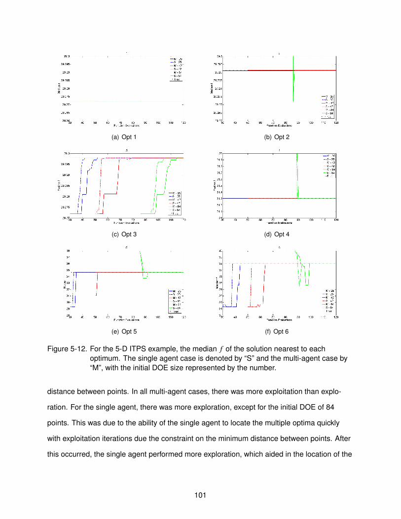
(a) Opt 1 (b) Opt 2

(c) Opt 3 (d) Opt 4

(e) Opt 5 (f) Opt 6

Figure 5-12. For the 5-D ITPS example, the median f of the solution nearest to eachoptimum. The single agent case is denoted by “S” and the multi-agent case by“M”, with the initial DOE size represented by the number.

distance between points. In all multi-agent cases, there was more exploitation than explo-

ration. For the single agent, there was more exploration, except for the initial DOE of 84

points. This was due to the ability of the single agent to locate the multiple optima quickly

with exploitation iterations due the constraint on the minimum distance between points. After

this occurred, the single agent performed more exploration, which aided in the location of the

101

most difficult optimum to locate, optimum 3. For the initial DOE of 84, the single agent had

fewer evaluations in which to locate all optima, so exploitation was dominant.

(a) Number of active agents (b) Number of iterations vs function evaluations

Figure 5-13. For the 5-D ITPS example, the number of active agents and the number ofiterations.

Figure 5-14. For the 5-D ITPS example, the percentage of points that were added inexploitation or exploration.

The superior performance by the single agent was also attributed to the accuracy of

its surrogate approximations. Fig. 5-15 compares the PRES S RMS of each surrogate for

the single and multi-agent cases. The PRES S RMS decreased with increasing number of

function evaluations after it initially increased. This was due to the placement of points

around the optima, which made the surrogate less accurate further from the optima. This led

to large errors when a point that was far away from other points was left out in calculating the

102

cross-validation error. As more exploration points were added, the PRES S RMS was reduced.

For the multi-agent case, we observed that the PRES S RMS increased through the function

evaluations. This was due to the large number of points put around the optima in exploitation

iterations, which outnumbered the exploration iterations.

Figure 5-15. Median PRES S RMS of the surrogates of the limit states for the 5-D ITPSexample

Figure 5-16 displays the error at 1000 test points eRMS . We observed much of the

same trends as with PRES S RMS , with the surrogates in the multi-agent case decreasing in

accuracy while the surrogates of the single agent cases increased accuracy.

5.8 Discussion

The single agent approach showed a clear advantage over the multi-agent method in

the ITPS example in Sec. 5.7. The single agent approach is simple : a global surrogate is

used and a constraint on the minimum distance between points is the only way to instigate

exploration of the design space. It is advantageous in its simplicity and ease of implemen-

tation, but its success depends on how well a single surrogate can approximate the global

behavior. The accuracy measures of the limit states for the ITPS example in Fig. 5-16 show

103

Figure 5-16. Median error at 1000 test points eRMS of the surrogates of the limit states for the5-D ITPS example

that the global surrogate of the single agent is indeed more accurate than several local sur-

rogates. Upon further investigation of the temperature and stress trends in the design space,

it was found that simple quadratic response surfaces over the design space were sufficient

approximations.

On the contrary, the modified Hartman 6 function presented in Sec. 5.6, for which

the unmodified version is often used as a benchmark function for surrogate-based global

optimization algorithms, is thought to be more complex compared to the ITPS example. The

error at test points (c.f. Fig. 5-9(b)) shows that the accuracy of the local surrogates is slightly

better than that of the single agent’s global surrogate. In this example, we observed that the

multi-agent method can be successful and efficient.

With that said, the comparisons made here in terms of efficiency are based on the

number of function evaluations. Ideally, the multi-agent partitioning method would be

parallelized such that a single iteration would involve simulatenous optimization in each

sub-region. That is, a single iteration could account for four function evaluations if there

104

are four agents working in four sub-regions. Therefore, in terms of efficiency the iterations,

which give an idea of wall clock time, should also be compared. For the ITPS example, the

single agent was shown to be more efficient at locating some optima by five to ten function

evaluations, but in terms of iterations the multiple agents are more efficient if the number of

function evaluations is translated into iterations by Fig. 5-13(b).

Otherwise, what does this say about this multi-agent algorithm? Based on these two

examples, the success rate and efficiency of the multi-agent method may be dependent on

having higher accuracy local surrogates compared to a global surrogate. Otherwise, simpler

algorithms may be more efficient. Further investigation on the need for local surrogates is

required, and a study that uses a global surrogate with the agent-based dynamic design

space partitioning is planned. It will allow us to study separately two ingredients that make

up the method investigated here: local versus global surrogate and space partitioning to

increase chances of visiting many basins of attraction leading to different local optima.

Additionally, the efficiency gains from parallelization should be investigated.

5.9 Summary and Discussion on Possible Future Research Directions

This chapter introduced a multi-agent methodology for optimization that dynamically

partitions the design space as to find multiple optima. Multiple designs provide insurance

against discovering that late in the design process a design is poor due to modeling errors or

overlooked objectives or constraints. The method used surrogates to approximate expensive

functions and agents optimized using the surrogates in the sub-regions. The centers of the

agents subregions moved to stabilize around optima, and agents were created and deleted

at run-time as a means of exploration and efficiency, respectively.

The method was applied to two examples, an analytical test function and a practical

engineering example. It was observed that for problems in which the behavior is simple to

approximate with a global surrogate, the simpler single agent is more efficient and successful

than the multiple agents. For the more complicated test function, in which local surrogates

were slightly more accurate, the multiple agents outperformed the single agent. These

105

results lead us to believe that the success of the current agent algorithm is dependent on

local surrogates being more accurate than a global surrogate.

This method aims too exploit the surrogate predictions by purely minimizing the function

rather than exploring the design space as evidenced by the comparison of the percentage

of iterations that put points near the optima. There is a focus on using surrogate predictions

to aid multiple cheap local searches throughout the design space. This is an important

differentiation between this algorithm and many global optimization algorithms that aim for

and tout the balance of exploitation and exploration.

Continuing research can focus on using a global surrogate with the dynamic partitioning

still in place. The reason for this is two-fold: (i) in the authors’ experience, there are few

situations in which local surrogates are significantly more accurate than a global surrogate,

(ii) the complication of managing points between sub-regions to create surrogates is

removed. Efficient Global Optimization[89] (EGO) is a popular global optimization algorithm

that uses a global surrogate and adds points based on the present best solution (the present

best data point). It is planned to modify the EGO algorithm for use with the dynamic design

space partitioning, in which each sub-region has its own present best solution.

The proposed agent optimization method also has a great potential for parallel com-

puting. As the number of computing nodes n increases, the calculation of the expensive

objective and constraints functions scales with 1/n in terms of wall-clock time. But the speed

at which problems can be solved then becomes limited by the time taken by the optimizer,

i.e., the process of generating a new candidate solution. In the algorithm we have developed,

the optimization task itself can be divided among the n nodes through agents. We plan to

explore how agents can provide a useful paradigm for optimizing in parallel, distributed,

asynchronous computing environments.

106

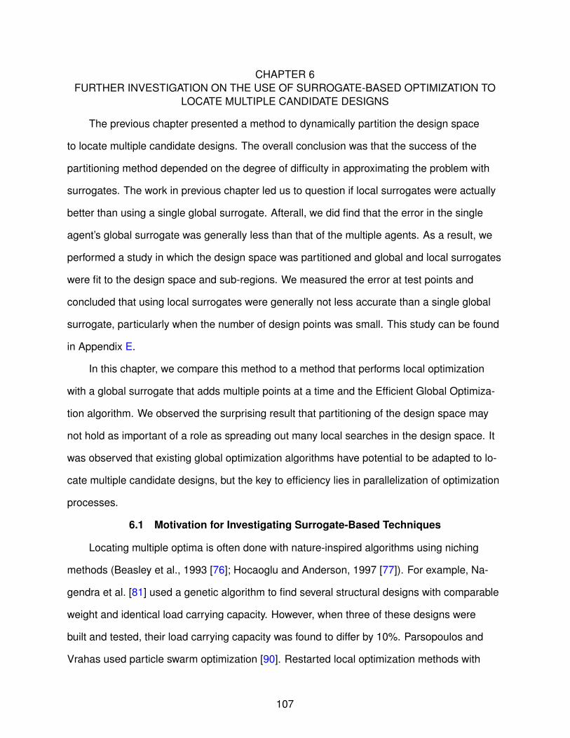
CHAPTER 6FURTHER INVESTIGATION ON THE USE OF SURROGATE-BASED OPTIMIZATION TO

LOCATE MULTIPLE CANDIDATE DESIGNS

The previous chapter presented a method to dynamically partition the design space

to locate multiple candidate designs. The overall conclusion was that the success of the

partitioning method depended on the degree of difficulty in approximating the problem with

surrogates. The work in previous chapter led us to question if local surrogates were actually

better than using a single global surrogate. Afterall, we did find that the error in the single

agent’s global surrogate was generally less than that of the multiple agents. As a result, we

performed a study in which the design space was partitioned and global and local surrogates

were fit to the design space and sub-regions. We measured the error at test points and

concluded that using local surrogates were generally not less accurate than a single global

surrogate, particularly when the number of design points was small. This study can be found

in Appendix E.

In this chapter, we compare this method to a method that performs local optimization

with a global surrogate that adds multiple points at a time and the Efficient Global Optimiza-

tion algorithm. We observed the surprising result that partitioning of the design space may

not hold as important of a role as spreading out many local searches in the design space. It

was observed that existing global optimization algorithms have potential to be adapted to lo-

cate multiple candidate designs, but the key to efficiency lies in parallelization of optimization

processes.

6.1 Motivation for Investigating Surrogate-Based Techniques

Locating multiple optima is often done with nature-inspired algorithms using niching

methods (Beasley et al., 1993 [76]; Hocaoglu and Anderson, 1997 [77]). For example, Na-

gendra et al. [81] used a genetic algorithm to find several structural designs with comparable

weight and identical load carrying capacity. However, when three of these designs were

built and tested, their load carrying capacity was found to differ by 10%. Parsopoulos and

Vrahas used particle swarm optimization [90]. Restarted local optimization methods with

107

clustering (Torn and Zilinkas [83], Torn and Viitanen [91]) have also been proposed for

finding many local optima. These methods require a large number of function evaluations,

which is prohibitively costly if the functions are expensive to evaluate.

To reduce the cost of optimization, surrogate models are often used (e.g. Jones et

al., 1998 [89], Alexandrov et al., 1998 [92]) to approximate the output of the simulations.

A surrogate (or metamodel) is an algebraic expression fit to a number of simulations.

Traditionally, the locations where simulations are carried out were selected independently

of the optimization, so that a surrogate fitting phase preceded the optimization phase. More

recently, global optimization algorithms that combine surrogate fitting and optimization have

gained popularity, most notably the Efficient Global Optimization (EGO) algorithm (Schonlau,

1997 [93], Jones et al., 1998 [89]). These use adaptive sequential sampling with points

added at locations with high potential of improving the design.

The research in the previous chapter described a methodology that sought to extend

adaptive sampling surrogate techniques to locate multiple optima. The proposed approach

was based on the conjunction of two principles to identify many candidate optima: i) dynamic

partitioning of the search space and ii) local surrogate approximations. In this chapter,

we examine the effectiveness of this approach in locating multiple optima along with two

methods: multiple starting points for local optimization and EGO, which is perhaps the

currently favored surrogate-based global optimization algorithm. Additionally, we compare

the use of global surrogate approximations in our previously developed approach in place of

local surrogates.

The next section of this chapter briefly summarizes the general idea behind surrogate-

based optimization to motivate the two approaches used as comparisons in this study,

multiple starting points of multiple local optimizations and the EGO algorithm, and describes

why they are interesting for this study. Section 6.3 compares these methods on two two-

dimensional numerical examples, minimization of the Branin-Hoo and Sasena functions.

108

6.2 Surrogate-Based Optimization

As described in Sec. 5.3, a surrogate is a mathematical function that (i) approximates

outputs of a studied model (e.g. the mass or the strength or the range of an aircraft as a

function of its dimensions), (ii) is of low computation cost and (iii) aims at predicting new

outputs [84]. The set of initial candidate solutions, or points, used to fit the surrogate is

called the design of experiments (DOE). Well-known examples of surrogates are polynomial

response surface, splines, neural networks, and kriging. Using the surrogate, a new point is

added based on some sampling criterion, and the surrogate is updated with the new point.

This process continues as dictated by some stopping criterion. The general procedure for a

problem with inequality constraints described by the limit states g proceeds as in Algorithm

6. The choice of how to use the surrogate prediction to find the optimum x∗ is considered in

Algorithm 6 Overall surrogate-based optimization1: t = 1 (initial state)2: while t ≤ tmax do3: Build surrogates f and g from (Xt,Ft,Gt)4: Optimization to find x∗ (see Algorithm 3)5: Calculate f (x∗) and g(x∗)6: Update database (Xt+1,Ft+1,Gt+1) ∪ (x∗, f (x∗), g(x∗))7: t = t + 18: end while

the next two sub-sections. There is the choice of simply solving original optimization problem

(i.e, minimizing f ) by solving Eq.(5–2), but there are many popular in-fill sampling criteria

that have been developed. The following two sub-sections expand on two options to find the

optimum x∗ .


f (x)


6.2.1 Multiple-Starting Points

In this research, we focus on local, gradient-based algorithms that remain efficient in

high dimensions, but have the disadvantage of being highly dependent on the starting point.

109

The choice of the starting point or “initial guess” can affect the ability of a local algorithm

to find the global optimum. Note that stochastic methods are also affected by the initial

configurations (e.g., the initial population in genetic algorithms). An optimizer that uses

gradients may not find the global optimum if its starting point is in the basin of attraction of a

poorer local optimum. To overcome this, multiple starting points are often used, in order to

take multiple trajectories to find a solution. Thus, the use of multiple starting points is good

practice when using such algorithms. There is the possibility of obtaining as many solutions

as starting points, though not all solutions may be unique as some starts may find the same

solution. The choice of starting points is important, and typically comes from sampling

methods (e.g., random sampling, grid sampling, Latin Hypercube sampling, etc.). There is

also the option of halting the optimization for poor trajectories.

Using multiple starting points is a relatively simple approach that can become pro-

hibitively costly if the objective function or constraints is expensive. In problems where the

cost of fitting and evaluating a surrogate is much less than the cost of evaluating the true ob-

jective function or constraints, using multiple starting points in conjunction with surrogates is

a viable approach to find multiple optima. Thus, we can investigate the use of multiple start-

ing points to find multiple optima by solving Eq.(5–2). In an iterative optimization scheme,

the single best solution of the starts or the multiple points resulting from multiple starting

points can added per iteration. Some random sampling is needed to prevent premature

convergence. This research investigates both surrogate and multi-start approaches.

6.2.2 Efficient Global Optimization

The Efficient Global Optimization (EGO) algorithm [89] is a sequential sampling global

optimization method. It starts by fitting a surrogate that comes with a prediction uncertainty.

After fitting the surrogate, the algorithm iteratively adds points to the data set in an effort to

improve upon the present best sample. In each cycle, the next point to be sampled is the

one that maximizes the expected improvement, E[I(x)]. Though another variant of the EGO

algorithm uses maximizes the probability of improvement on a targeted solution (EGO-AT

110

[51]), this work focuses on E[I(x)]. E[I(x)] is a measure of how much improvement upon

the present best sample we expect to achieve if we add a point. Rather than only searching

for the optimum predicted by the surrogate, EGO will also favor points where surrogate

predictions have high uncertainty. Therefore, EGO is able to balance exploitation of areas

with small objective function values and exploration of areas with high uncertainty. For further

details on the EGO algorithm, the reader may seek out one of the many papers on EGO,

notably [89, 93].

Since EGO tries to improve upon the present best solution, it may not be possible for it

to locate multiple optima if the values of the optima are very different or when some optima

are very poor. For example, if a local optimum of a function is already found, the expected

improvement may not be large enough to put a point in an area that contains another

optimum with a poorer objective function value. For this reason, for locating multiple optima

we restrict the comparisons of the EGO method to optima that are close in objective function

value. Additionally, EGO is capable of adding more than one point per iteration [50, 94], but

this research only considers the use of EGO in adding a single point per iteration.

6.3 Numerical Examples

This section compares the success and efficiency of the methods presented in this

chapter on locating multiple candidate designs for two numerical examples. Five methods

are compared: Two multi-agent methods that use dynamic partitioning but different surrogate

setups, two single agent methods that add one or three points per iteration, and EGO. The

methods considered are described in Table 6-1. The first case listed in Table 6-1 uses the

dynamic partitioning described in Ch. 5, but shares a global surrogate among the agents

rather than fitting a local surrogate to each agent. Using a global surrogate removes the

complication of exchanging points between sub-regions in order to avoid ill-conditioning

when fitting a local surrogates. Additionally, it may be more accurate than several local

surrogates as shown in the previous chapter. The method that uses local surrogates with

partitioning is still studied and listed as the second method in Table 6-1.

111

Table 6-1. Description of methodsMethod DescriptionAgents and Partitioning: Global(Sec. 5.4)

Uses multi-agents with dynamic partitioning. Agents use thesame global surrogate. As many points as agents are addedper iteration.

Agents and Partitioning: Local(Sec. 5.4)

Uses multi-agents with dynamic partitioning. Agent useslocal surrogate for its sub-region. As many points as agentsare added per iteration.

Single (Sec. 6.2.1) Single global surrogate agent adding one point per iteration.Multiple starts are used and the best point in terms of fea-sibility and objective function value is chosen. Explorationoccurs when a start gives a solution too near an alreadyexisting point. Exploration adds a point that maximizes theminimum distance from existing points.

Single: Multiple Points Per Iteration(MPPI) (Sec. 6.2.1)

Single global surrogate adding 3 points per iteration by 3start points for local optimization. Exploration occurs whena start gives a solution too near to an already existing point.Exploration adds a point that maximizes the minimum dis-tance from existing points.

EGO (Sec. 6.2.2) Global surrogate using EGO algorithm to add one point periteration

In all cases, the number of function evaluations was fixed at 100, including those

required for the initial design of experiments, for both examples. The number of points added

for the Single:MPPI case was set to three because it was observed that this was the mean

number of points added in the multi-agent cases for the same examples. Thus, we fixed

the number of points per iteration to three to provide a fairer comparison between the two

methods.

As different methods listed in Table 6-1 add a different number of points per iteration

(i.e., the Single:MPPI method adds three points per iteration, multi-agent method adds as

many points as agents, and Single and EGO cases only add one point per iteration), we

examine two values when comparing efficiency: number of function evaluations and number

of iterations. The advantage of adding multiple points per iteration as in the Single:MPPI and

multi-agent methods comes from parallelization between the processes that add the multiple

points. Thus, comparing these methods to ones that add only a single point per iteration

should be done based on the number of iterations rather than function evaluations. In the

112

results presented for the two examples in this section, we present both values. Note that for

the Single Agent and EGO cases the iterations and function evaluations are equal as both

only add a single point per cycle.


For the example considered in this study, there are no nonlinear constraints, so only the

objective function is approximated by surrogates.. The three possible surrogates are kriging

surrogates with quadratic, linear, or constant trend function. From this set, each agent chose

the best surrogate based on PRES S RMS . The set of surrogates and the minimum number of

points used to fit each surrogate is 1.5 x the number of coefficients of a quadratic response

surface. If the minimum number of points are not available when fitting local surrogates to

the sub-regions, points are borrowed from neighboring sub-regions in the order of increasing

distance to the agent center, and, if the requirement is still not met, then all available points

are used.

For the agent cases with partitioning, the parameters are provided in Table 6-2. For

Table 6-2. Multi-agent parameters for example problemsParameter ValueMax # of function evaluations 100Max # of agents 6Initial/Min # of agents 1Min distance between agent centers 10% of max possible distance in spaceMin distance between points 0.2% of max possible distance in spaceMin average silhouette 0.25Min # of points in each agent after creation 4Stagnation threshold 3Number of starting points for local optimization 10

distances, we consider the distance in the normalized space as a fraction of the maximum

possible distance between two points in the design space (e.g., for two-dimensional prob-

lems, we normalized by√

2). For example, we use this distance when considering the

minimum distance between centers and the minimum distance between data points as given

in Table 6-2.

113

The initial size of the DOE for both example problems was 12, with the points sampled

by Latin Hypercube Sampling. In each case given in Table 6-1, the results shown are the

median of 50 repetitions (i.e, 50 different initial DOEs). The local optimization problems were

solved with a sequential quadratic programming (SQP) algorithm [88]. DOEs are obtained

using Latin Hypercube sampling and the maximin criterion for five iterations.

6.3.2 Branin-Hoo Test Function

The first example is the minimization of the Branin-Hoo test function, a common

benchmark test function used in surrogate-based global optimization. It is given in Eq.(6–1).

f (x) =(x2 −

5.14π2 x2

1 +5π

x1 − 6)+ 10

(1 − 1

8π

)cos(x1) + 8 ≤ 0 (6–1)

The domain of the function is −5 ≤ x1 ≤ 10 and 0 ≤ x1 ≤ 15. There are three global optima

of the Branin-Hoo function, for which f = 0.40. A contour plot of the Branin-Hoo function is

shown in Fig. 6-1.

Figure 6-1. Contour plot of Branin-Hoo function showing three optima. For all optima,f = 0.40.

114

For 50 repetitions, the percentage of repetitions that successfully located a solution a

1% distance from the optimum is shown in Fig. 6-2, where the number of function evalua-

tions shown does not include the evaluations required for the inital DOE of 12 points. This

distance is the Euclidean distance normalized by the maximum possible distance between

points in the design space (here,√

2).

Figure 6-2. For the Branin-Hoo example, the percentage of 50 repetitions that found asolution within 1% distance from each optimum. For the cases that multiplepoints per iteration (agents and Single:MPPI) the value in terms of iterations isgiven by the solid lines and dashed lines for function evaluations.

115

First, if we make the comparison in terms of iterations, we observed that the Sin-

gle:MPPI method is quickly successful in 80% of the repetitions. However, to reach percent-

ages greater than 90%, the multi-agent method with the global surrogate located all optima

with the fewest iterations. In terms of the number of iterations, the general trend was that the

multi-agent method with a global surrogate reached 100% success with the fewest iterations

followed by either the multi-agent method with local surrogates or Single:MPPI, then the

single agent adding one point per iteration, and finally EGO. However, it should be noted that

EGO actually found solutions near to the optima with a small number of function evaluations,

but required more function evaluations to put a point within 1% of all optima as it was driven

to search other regions with higher expected improvement due to larger uncertainty in the

surrogate.

When considering the number of function evaluations, which does not account for the

parallelization in the addition of multiple points per iteration, the single agent is the most

efficient while the multi-agent method with local surrogates is the least efficient with the other

methods falling in between.

Figure 6-3 displays the median objective function value with iterations and function

evaluations for the solution nearest to each optimum. We observed that the Single:MPPI

method had a median f value closest to the global optimum of f = 0.39 with the fewest

iterations, and even the fewest function evaluations as compared to the other cases. In

fact, the Single:MPPI method considering function evaluations was even more efficient than

agents in terms of iterations. Otherwise, we observed much of the same trends between the

one-point-per iteration methods and the agent methods.

116

Figure 6-3. For the Branin-Hoo example, the median objective function of the solutionnearest to each optimum. For the cases that multiple points per iteration (agentsand Single:MPPI) the value in terms of iterations is given by the solid lines anddashed lines for function evaluations.

Figure 6-4 displays the placement of points in the design space after 100 total function

evaluations for each method for a single repetition. It is observed that the single agent

method put many points around the optima and only few points in the rest of the design

space in exploration. In contrast, the Single:MPPI method both clustered points around

the optima and filled the design space. The EGO method did not put nearly as many

points around the optima and put many points in exploration in the design space, which is

consistent with its goal of searching in areas with promising improvement.

117

Figure 6-4. For the Branin-Hoo example, the plot of the points found by different methods forone repetition

The placement of points for the multi-agent cases was quite different when using global

and local surrogates. While both put many points around each optimum, local surrogates

resulted in many points away from the optima. This was partially due to the error in the

surrogate, which predicted good objective function values away from the optima. To measure

the error, we calculated the error at 1000 test points by erms. The erms normalized by the

estimated range of the Branin-Hoo function is provided in Fig. 6-5.

118

Figure 6-5. For the Branin-Hoo example, the error at 1000 test points with erms as thepercentage of the estimated range of the function

It was observed that local surrogates were the least accurate, while the single global

surrogate in the Single:MPPI method had less than 1% error after 20 function evaluations.

After observing that agent method using the global surrogate was only slightly less

efficient than using a single agent adding 3 points per iteration, we examined the case with a

constant 3 agents (3 sub-regions) and compared it to the Single:MPPI method adding three

points per iteration. This simulates a case when three computing nodes are available, and all

resources are used by assigning one agent to one node. Recall, that we previously set the

initial number of agents at one, and let the number of agents evolve over time while setting

the maximum number of agents at six. Figure 6-6 displays the percentage of 50 repetitions

that located a solution with 1% distance from each optimum with iterations and function

evaluations.

119

Figure 6-6. For the Branin-Hoo example, a comparison between the percentage of 50repetitions that found a solution within 1% of the each optimum for the a constant3 agents with a global surrogate and the Single: MPPI approach. Note that bothmethods add three points per iteration.

It was observed that the rate at which 100% success was achieved was quite similar

between the two cases, with the agent method slightly more efficient. Therefore, efficiency

may be increased by maximizing the use of computational resources by setting a constant

number of agents rather than letting the number of agents evolve over time. However, it

should be noted that Single:MPPI only allows three starting points in the design space,

whereas the three agents each have ten starting points in the design space, for a total of

30 starting points. Thus, it is not entirely unexpected that the three agents achieve success

at a slightly higher rate as they choose from 10 points to find the best point per iteration as

compared to one. This shows that spreading out a large number of local searches in the

design space, which is done by adding multiple points per iteration with the single global

surrogate, may simply be as effective as partitioning of the design space.

120

6.3.3 Sasena Test Function

The second example problem, is the minimization of the Sasena function, which was

used by Sasena under the name “mystery” function due to its unknown origin[95].

f (x) = 2 + 0.01(x2 − x21)2 + (1 − x1)2 + 2(2 − x2)2 + 7sin(0.5x1)sin(0.7x1x2) (6–2)

The domain of the function is 0 ≤ x1, x2 ≤ 5. A contour plot of the Sasena function is

shown in Fig. 6-7. There are four optima, as shown in the figure, but the values of optima 3

( f = 12.7) and 4 ( f = 33.2) are 40% and 90% from the global optimum ( f = −1.46) in terms

of the range of the function (38.6). Optimum 2 ( f = 2.87), which has 11% difference from the

global optimum is the only competitive optimum. Therefore, it is expected that the methods

compared here are only effective at locating optimum 1 and 2.

Figure 6-7. Contour plot of Sasena function showing four optima

121

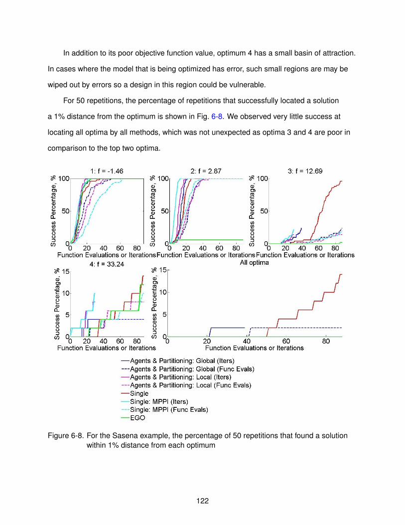
In addition to its poor objective function value, optimum 4 has a small basin of attraction.

In cases where the model that is being optimized has error, such small regions are may be

wiped out by errors so a design in this region could be vulnerable.

For 50 repetitions, the percentage of repetitions that successfully located a solution

a 1% distance from the optimum is shown in Fig. 6-8. We observed very little success at

locating all optima by all methods, which was not unexpected as optima 3 and 4 are poor in

comparison to the top two optima.

Figure 6-8. For the Sasena example, the percentage of 50 repetitions that found a solutionwithin 1% distance from each optimum

122

When the comparison is made in terms of number of iterations, the methods that call for

parallelization of the optimization processes (i.e, the multi-agent methods and Single:MPPI)

outperform the one-point-per-iteration single agent and EGO algorithm. The Single:MPPI

method again achieves a high percentage of successes with only a few iterations for optima

1 and 2, but the rate of success for both multi-agent cases is comparable for the global

optimum. Another thing to note is the comparable performance of the multi-agent method

with local surrogates compared to the global surrogate, which was not observed in the

Branin-Hoo example.

It was also observed that EGO was efficient in locating the global optimum, but only had

under 10% success in locating optimum 2. Based on this example, the current implementa-

tion of EGO has less potential to be successful in locating multiple optima when the optima

are not almost equal.

When comparing the efficiency in terms of number of function evaluations, the one-

point-per-iteration single agent is the most efficient. In fact, the single agent is able to locate

optimum 3 in 90% of the repetitions. This is because the single agent locates optima 1 and 2

in early iterations, and is able to put points in the other parts of the space to locate optimum

3.

Figure 6-9 displays the median objective function value with iterations and function

evaluations for the solution nearest to each optimum. We observed that the Single:MPPI

method had a median f value closest to optima 1, 2, and 3 with the fewest iterations, and in

most cases, the fewest function evaluations. Additionally, it was observed that for optimum 3,

the median f for the Single:MPPI method is quite close to the true value, which was not clear

when examining the success percentage. For optimum 4, it was observed that the nearest

solution for all cases except Single:MPPI had a median f of 35.9, which corresponds to a

space-filling point at the corner of the design space at (5, 5).

123

Figure 6-9. For the Sasena example, the median objective function of the solution nearest toeach optimum. For the cases that multiple points per iteration (agents andSingle:MPPI) the value in terms of iterations is given by the solid lines anddashed lines for function evaluations.

The error of the surrogate approximations at 1000 test points is shown in Fig. 6-10. As

in the Branin-Hoo example, it is observed that the single surrogate with multiple points per

iterations was the most accurate and the local surrogates from the multi-agent system were

the least accurate.

Figure 6-10. For the Sasena example, the error at 1000 test points with erms as thepercentage of the estimated range of the function

124

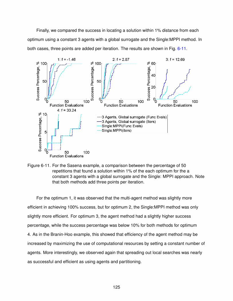
Finally, we compared the success in locating a solution within 1% distance from each

optimum using a constant 3 agents with a global surrogate and the Single:MPPI method. In

both cases, three points are added per iteration. The results are shown in Fig. 6-11.

Figure 6-11. For the Sasena example, a comparison between the percentage of 50repetitions that found a solution within 1% of the each optimum for the aconstant 3 agents with a global surrogate and the Single: MPPI approach. Notethat both methods add three points per iteration.

For the optimum 1, it was observed that the multi-agent method was slightly more

efficient in achieving 100% success, but for optimum 2, the Single:MPPI method was only

slightly more efficient. For optimum 3, the agent method had a slightly higher success

percentage, while the success percentage was below 10% for both methods for optimum

4. As in the Branin-Hoo example, this showed that efficiency of the agent method may be

increased by maximizing the use of computational resources by setting a constant number of

agents. More interestingly, we observed again that spreading out local searches was nearly

as successful and efficient as using agents and partitioning.

125

6.4 Discussion and Summary

This chapter provided a comparison of the success and efficiency in locating multiple

optima by different surrogate-based optimization methods. Our previously developed multi-

agent method that dynamically partitions the design space was compared against the EGO

algorithm and a simple method that uses multiple starts in the design space to either add

one or several points in an iteration. It was observed that EGO has the potential to locate

multiple optima when optima functions values are similar, while the other methods presented

here have this ability for optima that are within 11% of the range of the function. In practice,

this is an ideal scenario as one would not want to waste resources on searching for poor

optima.

The most efficient methods of those studied here aimed to take advantage of parallel

computing for optimization. The use of multiple starting points for local optimization and

adding multiple points per cycle proved to be a simple yet efficient method that warrants fur-

ther research. The multi-agent approach, which involves optimization in several dynamically

changing sub-regions in parallel, was also shown to be efficient in locating competitive op-

tima. This shows that the benefit of partitioning the design space is that it helps spread local

searches throughout the design space, and also increases the potential for parallelization.

We observed that the error in local surrogate approximations by the multiple agents

was larger compared to a global surrogate. Additionally, we did not observe that local

surrogates outperformed the global surrogate in either test problem, which supports the

study in Appendix E that compared the accuracy of global to local surrogates for several

test functions. For these reasons, it may be possible to only use a global surrogate, which

removes the complication of exchanging points between agents to fit local surrogates.

In the future, a more in-depth look at the advantages of using multiple points per

iteration can be studied. There is the possibility to explore asynchronous agents that partition

the starting points for local optimization in the space and update the global surrogate as new

points are added.

126

CHAPTER 7CONCLUSIONS

The initial stages of design include the formulation of the optimization problem, including

objective functions and constraints, and often include building a computational model with

which to perform the initial design optimization. However, there is uncertainty in the process,

which stems from the inability to perfectly formulate the optimization problem, inherent

uncertainties in the design, and the uncertainties in the computational model. Tests and

redesign are often performed on candidate designs, which allows for the identification of

dangerous designs that can be redesigned and also provides measures by which to calibrate

computational models. This research considers two areas of the design of engineering

systems: 1) the trade-off of the effect of a test and post-test redesign on reliability and cost

and 2) the search for multiple candidate designs as insurance against unforeseen faults in

some designs.

The main contributions of this research are as follows:

1. A methodology to quantify the effect of a single future test and redesign on perfor-mance and cost

2. An investigation on how to trade off performance and development costs by includ-ing the effect of a single future test and redesign, and additionally how this allowscompanies probabilistically set design and re-design rules

3. A dynamic partitioning method of the design space that combines surrogates and localsearch to locate multiple candidate designs

First, a methodology to quantify the effect of a single future test and redesign on

performance and cost was presented for fixed design and redesign rules. This method was

based on sampling computational and experimental errors to simulate alternative future

test outcomes, for which the decision to design or redesign was made. Two methods of

calibration and redesign were presented. In one method, a simple correction factor based

on the ratio of the simulated experimental measurement to the predicted value from the

computational model was used in calibration, and redesign was performed deterministically

to restore the initial level of safety of the design as dictated by a required safety margin. The

127

second method used Bayesian updating to update the initial computational error distribution

and redesigned to meet a targeted reliability level given the updated error distribution. It was

observed these methods provided estimates of the distribution of the probability of failure

and performance of a design after test and redesign.

As an extension of the previous research, it was shown that the probabilistic quantifi-

cation of the effect of the future test and redesign could be used to trade off performance

and development costs by setting design and redesign rules. This research considered

deterministic design and redesign rules, which are representative of current design practice

used presently in industry. In this study, it was shown that the optimal trade-off called for

initially conservative designs with large safety margins, which were made less conservative

but with increased performance with increasing redesign (development) costs. This result

was compared to the opposite approach in which a minimum required safety margin is given,

which reflects the practice of regulatory agencies providing minimal required safety margins

and factors.

The third area of research focused on locating multiple candidate designs by a combi-

nation of dynamic design space partitioning and surrogate-based optimization by mutliple

local searches in sub-regions. This research focused on how to partition the design space

such that the center of each region was located on a local optimum, while creating regions

to explore the design space and merging regions that converged to the same area. The

coordination between regions for surrogate-fitting, optimization, and exchange of design

points was inspired by multi-agent approaches seen in distributed optimization algorithms

that take advantage of the decomposition of the optimization formulation. This research

mainly explored the use of local and global surrogates, where a local surrogate was used in

each region of the design space in order to provide a more accurate approximation of the

local behavior. This method was compared to a relatively simple approach in which a single

surrogate using multiple starting points for local optimization over the entire design space.

It was observed that the success of the partitioning method was primarily due to the use

128

of multiple starting points for local searches in the space. In effect, this led the multi-agent

method to exploit regions of predicted low function value and only explore sparsely populated

regions of the design space when this was not possible. Additionally, it was found that the

success and efficiency of the partitioning with local versus global surrogates method may

be dependent on the degree of difficulty in approximating the behavior with surrogates. For

several test problems, it was found that using local surrogates was not as advantageous as a

single global surrogate. It was also observed that there may be large gains in efficiency if the

optimization in the regions is parallelized.

7.1 Perspectives

Based on the research presented in this dissertation, future research includes three

tasks: 1) efficient identification of individual local optima, 2) establishing the range of accept-

able designs based on the vulnerability of the best optima 3) distributed implementation of

the methods.

7.1.1 Efficient Identification of Individual Local Optima

While the research in Ch. 5 have shown that locating multiple optima with surrogates

is a promising direction of research, there are remaining formidable challenges that can be

addressed.

7.1.1.1 Isolating basins of attraction

The goal is to isolate and characterize the basins of attraction of each local optimum.

In past implementations, only the performance of design points was considered to center

the agents. Yet, one sub-region may span two or more basins of attraction, such that a local

optimum may be missed because the optimization repeatedly finds the optimum with the

lower objective function value. There is a need to develop an efficient method to detect that a

sub-region contains more than one acceptable optimum.

Proposed approach. Since the center of the sub-region is at the best point in the

sub-region in terms of the objective function value (and feasibility in constrained problems),

the poorer other optima are not explicitly identified. The proposed improvement is to tag

129

the potential local optima that are found using multi-start local methods on the surrogates

according to whether or not they satisfy optimality conditions.There should also be a

distinction between optima inside a sub-region and optima at the boundary of a sub-region,

as the boundaries between sub-regions are artifacts of the method but not real design

constraints. For example, if there are three optima in two sub-regions, two centers may

be located at the two centers, but one basin of attraction may span both sub-regions.

Recognizing the position of the points at the boundary along with tagging the potential

optima may aid in the creation of sub-regions that will lead to the isolation of basins of

attraction.

7.1.1.2 Suspending or allocating few resources to unpromising sub-regions

Some sub-regions may appear to have local optima that are too poor to be worthwhile.

It is important to not write-off these regions completely as they may contain a good optimum

in a very narrow basin of attraction. However, search in the sub-region may be suspended

or fewer expensive function evaluations may be allocated to this region until more promising

sub-regions are explored. Developing such a criterion is an important step to make this type

of method more efficient.

Proposed approach. A common stopping criterion found in global optimization is based

on the convergence of the objective function value [96, 97]. For this research, it is proposed

that the criterion to suspend search in a sub-region or allocate fewer resources to the region

is based on objective function value, feasibility, size of the domain, and its vulnerability to

modeling errors. Such a criterion would differentiate between relatively small regions with

poor objective function values in which search may be suspended, and large regions with

small function values which may still benefit from further exploration to identify more optima.

In the DIRECT method, Jones et al. [98] allocated resources in the regions of the design

space that represented the best compromises, according to Pareto dominance, between the

objective function and the size of the unexplored neighborhood. It is proposed to extend such

a multi-criterion rationale in guiding the search considering i) the performance of the designs

130

and ii) the density of the starting points in the agent sub-regions, and (iii) vulnerability indices

as the criteria for allocating computing resources. With such an approach, narrow basins

of attraction will be found early if they are in a region of good objective functions, and vice

versa, which matches the practical interest they may have (an optimum in a narrow valley

surrounded by poor performance designs is likely to be too unstable for practical purposes).

7.1.2 Vulnerability Analysis and Range of Acceptable Objective Functions

Chapters 3 and 4 presented a methodology that sought to model the effect of errors

on the eventual mass of a design by simulating futures where the errors force redesign

based on bounds on modeling errors. This was done assuming that the errors are small to

moderate and future tests that will reveal them to require only re-calibration of the analysis.

The research demonstrated that a design can significantly change when considering errors

in combination with tests and redesign to check for and compensate for these errors. By

considering the effect of errors and simulating possible futures, the vulnerability of a design

to be affected by errors can be measured by the probability of redesign (the probability that

the design does not meet requirements), while performance measures, such as mass, give

an indication of the extent of the changes to the design that have to be made to compensate

for the errors.

Additional research in this area has extended this methodology to multiple failure modes

[68] and also sought to model the effect of unexpected large errors [99]. This work can

be extended to allow the comparison of multiple designs and to estimate the probability of

islands of feasibility being wiped out.

Proposed approach that takes advantage of modeling of the effect of future tests

and redesign. The present approach is based on Monte Carlo simulations of multiple

possible futures associated with different error magnitudes. The associated computational

cost is high, and therefore not feasible to be incorporated inside a global optimization

algorithm. We propose to develop approximate estimates of the mean objective function

increment after future redesign as well as its standard deviation. This will be based on a

131

simple re-calibration approach that we have explored in Ch. 3. It is also proposed to develop

estimates of the probability that an island of feasibility associated with a given local optimum

will completely disappear. This can happen when the island is narrow due to small errors

that are within the expected range anticipated by the designer. For example, for the example

presented in Ch. 5, an error of 12 K in the temperature model of the ITPS will wipe out

Region 2 of Figure 3 due to thermal failure. However, feasible regions may also disappear

due to unexpected appearance of overlooked failure modes or objective functions. It is

proposed to allow designers to assign such probabilities based on the closeness of the

design to their past experience. Designs that appear to be mere refinements of previous

experience may be assigned low probability while designs that look very different may be

assigned higher probabilities.

132

APPENDIX ACOMPARISON OF BAYESIAN FORMULATIONS

In a rigorous formulation of the likelihood function, we would calculate the conditional

probability of obtaining the measured temperature when the true temperature of the test

article is T , as shown in Eq.(A–1)

ltest(T ) =

1

0.14T if∣∣∣T−Tmeas

T

∣∣∣ ≤ 0.07;

0 otherwise.(A–1)

In the illustrative example in Section 3.3.2.1, we simplified this formulation so that we

calculated the conditional probability of obtaining T given Tmeas, as shown in Eq.(3–16). In

Fig.A-1, we compare the two likelihood functions and the resulting updated distribution of

f updtest,Ptrue for the case in the example.

Figure A-1. Illustrative example of Bayesian updating using the likelihood about Tmeas (top),and the likelihood about T (bottom)

The figures show only a small difference in the bounds of the updated temperature

distribution and the values of the pdf. A comparison is shown in Table A-1.

133

Table A-1. Comparison of f updtest,Ptrue with different formulations of the likelihood function

Comparison ltest(T ) about Tmeas ltest(T ) about TBounds where updated distribution is nonzero [0.9765, 1.1] [0.9813, 1.1]Max f upd

test,Ptrue and location 8.1 on [0.9765, 1.1] 8.9 at T = 0.9813

134

APPENDIX BEXTRAPOLATION ERROR

In this research, it was assumed the variation in the magnitude of the extrapolation

error eextrap was linear with the distance of the design from the test design. The choice of this

extrapolation error is very much up to the analyst, as it is a measure in the variation of the

errors from the updated Bayesian estimate away from the test design. Here, we examine the

effect of an assumption that the extrapolation error is quadratic, as expressed in Eq.(B–1).

eextrap = (eextrap)max

(∥d − dtest∥∆dlim

)2

(B–1)

For the example problem in Section 3.5, we estimated eextrap to be 2% when d is

changed by ±10% from dtest. With the quadratic extrapolation error, this is expressed as in

Eq.(B–2). Because of this requirement, the magnitude of the quadratic extrapolation error

is smaller for designs at a distance less that ±10% away from the test design but larger at

greater distances compared to the linear variation. We present this comparison in Fig.(B-1).

Examining the same 10000 possible outcomes of the future test with probabilistic redesign

(p f ,target = 0.01%), the results in Table B-1 were obtained.

eextrap = 0.02(∥d − dtest∥0.1∥dtest∥

)2

(B–2)

The results show that there is improved agreement between the true and analyst

estimated probabilities of failure, as well as a slightly decreased mass and variation in the

mass, with the quadratic variation in extrapolation error. Since the extrapolation error is

smaller at a distance less than ±10% away from the test design, the agreement between the

true and analyst-estimated probabilities of failure is better with the quadratic extrapolation

error. However, the agreement still suffers due to the large magnitude of the extrapolation

error at distances greater than ±10%.

135

Figure B-1. Comparison of the eextrap with linear and quadratic variation with the distance ofthe design from the test design (test design is d = 71.3 mm)

136

Table B-1. Calibration by the Bayesian updating approach with probability of failure based redesign (p f ,target = 0.01%), quadraticextrapolation error, and no bounds on redesign dS

Variation in eextrap with ds Parameter Original Mean Standard Deviation Minimum Maximum

Linear


Quadratic


137

APPENDIX CSIMULATING A TEST RESULT AND CORRECTION FACTOR θ

As described in Sec. 4.3, a test is performed to verify a design, and the test is performed

on a test article denoted by dtest and rtest to find the experimentally measured temperature

∆Tmeas. For this design, we can calculate ∆Tcalc(dtest, rtest). We can relate both the mea-

sured and calculated temperatures to the true temperature of the test article by the true

experimental and computational errors as

Ttest,true = T0 + ∆Tmeas(dtest, rtest)(1 − ex,true) = T0 + ∆Tcalc(dtest, rtest)(1 − ec,true) (C–1)

Rearranging this equation, we arrive at the correction factor θ = 1−ec,true

1−ex,true.

In this section, it is shown that the mass before and after redesign can be found

using a surrogate that is a function of safety margin and difference between the allowable

temperature Tallow and initial temperature T0. A surrogate of of the probability of failure that is

a function of the same two variables and the computational error ec can be made as well.

As shown in Eq.(4–2), the initial design satisfies

T0 + ∆Tcalc(d, r) + S 1 = Tallow (C–2)

Rearranged so that ∆Tcalc(d, r) is on the left hand side, this becomes

∆Tcalc(d, r) = (Tallow − T0) − S 1 (C–3)

By Eq.(4–5)the redesign should satisfy

T0 + θ∆Tcalc(d, r) + S 4 = Tallow (C–4)

which rearranged so that ∆Tcalc(d, r) is on the left hand side is

∆Tcalc(d, r) = (Tallow − T0)/θ − S 4/θ (C–5)

138

By Eqs.(C–3) and (C–5), the two are equivalent if (Tallow − T0) = [(Tallow − T0)/θ]a f terredesign and

S 1 = S 4/θ. Therefore, ∆Tcalc, along with its corresponding mass and probability of failure, is a

function of (Tallow −T0) and S , where the values with and without redesign are related through

θ. This allows the mass to be calculated simply using surrogates with the inputs (Tallow − T0)

and S . A surrogate to obtain the probability of failure can also be obtained by including the

computational error ec as an input.

Note that ∆Tcalc(d, r) does not need to be calculated because, for a given (Tallow − T0)

and S 1, we can find ∆Tcalc(d, r) by

(Tallow − T0) − S 1 = ∆Tcalc(d, r) (C–6)

When the correction is applied, then we evaluate if redesign is necessary by

Redesign if: (Tallow − T0) − θ[(Tallow − T0) − S 1] ≤ S 2

or (Tallow − T0) − θ[(Tallow − T0) − S 1] ≥ S 3

(C–7)

which simplifies to

Redesign if: (Tallow − T0)(1 − θ) + θS 1 ≤ S 2

or (Tallow − T0)(1 − θ) + θS 1 ≥ S 3

(C–8)

Kriging surrogates (quadratic trend function with a Gaussian correlation model) were

used for the surrogates of the mass and reliability index. The accuracy of the surrogates was

measured by the PRES S RMS , a leave-one-out cross validation error measure, and the eRMS

at 50 test points. A summary of the surrogates is provdied in Table C-1.

Table C-1. Summary of surrogatesSurrogate Inputs # of Points for Fitting PRES S RMS

1(%) Test eRMS2(%)

β (Tallow − T0) , S , ec 40 11 7m (Tallow − T0) , S 20 0.5 0.1

1PRES S RMS =√

1peT

XVeXV , where p is the number of points used for fitting and eXV isthe vector of the difference between the true value and the surrogate prediction

2 eRMS =√

1qeT

testetest, where q is the number of test points and etest is a the vector ofthe difference between the true value and the surrogate prediction

139

APPENDIX DEFFECT OF ADDITIONAL UNCERTAINTIES

In Ch. 4 we formulated the probability of failure is calculated with the limit state g as

gtrue = Tallow − Ttrue(d, r, v0) (4–7)

where

Ttrue(d, r, v0) = T0(1 − v0) + (1 − ec,true)∆Tcalc(d, r) (4–6)

Given the uncertainties in v0, ∆Tcalc, ec, and Tallow, we can calculate the variance of the limit

state as

σ2g,current = T 2

0σ2v0+ σ2

∆Tcalc+ ∆T 2

calcσ2ec+ σ2

∆Tcalce2

c + σ2ecσ2∆Tcalc+ σ2

Tallow(D–1)

We use the subscript “current” to denote this as the limit state that is used in Ch. 4.

In Ch. 3 and in [100], the limit state was formulated as

gprevious = T detallow − Tcalc(d, r)(1 − ec) (D–2)

for which the variance is

σgprevious = σ2Tcalc+ T 2

calcσ2ec+ σ2

Tcalce2

c + σ2ecσ2

Tcalc(D–3)

In Ch. 4, we included the additional uncertainties in the initial temperature, calculated change

and temperature, and allowable temperature to form a more realistic problem.

Let us consider two cases where redesign the combination of the test and redesign

reduces the standard deviation of ec for the design listed in Table D-1. The values of the

uncertain variables are given in Table 3-1, for which the variables involved in the calculation

of Tcalc and ∆Tcalc result in a standard deviation of 12.4 K in these values.

Using Eqs.(D–3) and (D–1), we calculate the standard deviation of the limit state g

as shown int Table D-2. It was observed that the additional uncertainties, particularly the

uncertainty in Tallow, reduced the effect of the test and redesign’s reduction of σec on the

reduction of the standard deviation of the limit state. The reductions were more than two

140

Table D-1. Values of the uncertain variables in the limit states.Distribution Before Redesign After Redesign Case 1 After Redesign Case 2T0 300 (deterministic)Tcalc N(550,12.42)∆Tcalc N(250,12.42)Tallow LN(660,162)ec N(0,0.0692)1 N(0,0.06212)2 N(0,0.0352)3

1 This is the standard deviation of the normal distribution that is equivalent tothe uniform distribution of ec between ±0.12 (i.e., 0.12√

3).

2 In case 1, redesign causes a 10% reduction in standard deviation of ec.3 In case 2, redesign causes a 50% reduction in standard deviation of ec.

Table D-2. Standard deviation of the limit states before and after redesign. Note that thenominal value of ec is 0.

Distribution Before Redesign After Redesign Case 1 After Redesign Case 2(% change) (% change)

σgprevious 39.9 36.4 (-9%) 22.7 (-43%)σgcurrent 26.8 25.7 (-4%) 22.2 (-17%)

times larger using the previous formulation, which accounts for the differences in mean and

95th percentile of the probability of failure we observed in Ch. 4 and the work in the Ch. 3.

141

APPENDIX EGLOBAL VS LOCAL SURROGATES

In this appendix, the accuracy of a single global surrogate over the design region

is compared to several local surrogates fit in sub-regions. In this study we examine five

two-dimensional functions and one six-dimensional function. Four of the two-dimensional

functions were taken from a study by Xiong et al. [101], in which some functions were

examined because they had visible non-stationary behavior (varying levels of smoothness

or bumpiness in the space) such that the stationary assumption of a stationary covariance

structure that underlies kriging does not hold. The six functions studied are listed below,

where the functions that come from the study [101] are labeled.

1. Branin-Hoo:

f (x) =(x2 −

5.14π2 x2

1 +5π

x1 − 6)+ 10

(1 − 1

8π

)cos(x1) + 8 ≤ 0

x1ϵ[−5, 10], x2ϵ[0, 15](6–1)

2. Sasena (“mystery function” in [101]):

f (x) = 2 + 0.01(x2 − x21)2 + (1 − x1)2 + 2(2 − x2)2 + 7sin(0.5x1)sin(0.7x1x2)

x1,x2ϵ[0, 1](6–2)

3. Function 3 [101]:

f (x) = sin(1

x1x2), x1,x2ϵ[0.3, 1] (E–1)

4. Function 4 [101]:f (x) = x1exp(−x2

1 − x22), x1,x2ϵ[−2.5, 2.5] (E–2)

5. Function 5 [101]:

f (x) = cos(6(x1 − 0.5)) + 3.1|x1 − 0.7| + 2(x1 − 0.5) + · · ·

7sin(1

|x1 − 0.5| + 0.31) + 0.5x2 x1,x2ϵ[0, 1]

(E–3)

6. Hartman 6:

f (x) = −q∑

i=1

aiexp

− m∑j=1

bi j(x j − di j)2

xiϵ[0, 1]

(E–4)

In this instance of Hartman 6, q = 4 and a =[1.0 1.2 3.0 3.2

]where

142

B =

10.0 3.0 17.0 3.5 1.7 8.00.05 10.0 17.0 0.1 8.0 14.03.0 3.5 1.7 10.0 17.0 8.0

17.0 8.0 0.05 10.0 1.0 14.0

D =

0.1312 0.1696 0.5569 0.0124 0.8283 0.58860.2329 0.4135 0.8307 0.3736 0.1004 0.99910.2348 0.1451 0.3522 0.2883 0.3047 0.30470.4047 0.8828 0.8732 0.5743 0.1091 0.0381

The test procedure can be described as follows:

1. Generate a DOE using LHS

2. Fit a global surrogate

3. Fit local surrogates: Partition the design space into n regions by choosing c randomcenters from the DOE and partition the space based on the distance of a point to thenearest center. Fit a surrogate in each region. Repeat for 10 random sets of centers.

4. Calculate error at 500 test points and then calculate eRMS for global and local surro-gates

This process is repeated for 50 DOEs for the size of 12, 22, 31, 41, and 50 points for the

two-dimensional functions and 56, 80, 103, 127, and 150 for Hartman 6.

Due to the randomness in choosing centers, it is possible that some sub-regions may be

small and hold only a small number of points. In order to avoid ill-conditioning in these cases,

the nearest points from neighboring sub-regions used to build the surrogate. For both the

quadratic response surface and kriging, the minimum number of points used to fit a surrogate

was 12 for the two-dimensional problems and 56 for the six-dimensional problem.

Figure E-1 shows the test error at 500 test points, measured by the root mean square

of the error, and normalized by the mean of the available data. Overall, it was observed

that the kriging surrogate was more accurate than the quadratic response surface. It was

observed that a global kriging surrogate was clearly more accurate for the Sasena function

and function 4. For the other test problems, there was only a small observable distance

in accuracy between global and local kriging, with global kriging seemingly slightly more

accurate. At large DOEs, there is less of a difference in accuracy between global and local

surrogates.

143

Figure E-1. For 4 equal sized regions, a comparison of the test error for global and localkriging surrogates.

From this study, we can conclude that several local surrogates generally do not carry an

advantage over local surrogates. However, in this study, the sub-regions did not result from a

partitioning scheme that considered function value; they were the results of randomly placed

centers in the design space. It is not clear if dividing the design space into partitions that

captured local behavior would improve the accuracy of the surrogate.

Additionally, knowing how to smartly split the design space would require an accurate

estimation of the global behavior, which would come from an accurate global surrogate. In

terms of optimization, accurate global surrogates could lead to a switch from optimization

with a surrogate to local optimization with the true function in interesting regions rather

than forming a local surrogate at the interesting region and continuing optimization with a

surrogate.

144

REFERENCES

[1] Oberkampf, W. L., Deland, S. M., Rutherford, B. M., Diegert, K. V., and Alvin, K. F.,“Error and Uncertainty in Modeling and Simulation,” Reliability Engineering andSystem Safety, Vol. 75, 2002, pp. 333–357.

[2] Acar, E., Haftka, R. T., and Kim, N. H., “Effects of Structural Tests on Aircraft Safety,”AIAA Journal, Vol. 48, No. 10, 2010, pp. 2235–2248.

[3] Melchers, R. E., Structural Reliability Analysis and Prediction, New York: Wiley, 1999.

[4] Fujimoto, Y., C., K. S., Hamada, K., and Huang, F., “Inspection Planning Using GeneticAlgorithm for Fatigue Deteriorating Structures,” International Offshore and PolarEngineering Conference, Vol.4, International Society of Offshore and Polar Engineers,Golden, CO, 1998, pp. 99–109.

[5] Toyoda-Makino, M., “Cost-based Optimal History Dependent Strategy for RandomFatigue Cracks Growth,” Probabilistic Engineering Mechanics, Vol. 14, No. 4, Oct.1999, pp. 339–347.

[6] Garbatov, Y. and Soares, C. G., “Cost and Reliability Based Strategies for FatigueMaintenance Planning of Floating Structures,” Reliability Engineering and SystemsSafety, Vol. 73, No. 3, 2001, pp. 293–301.

[7] Kale, A., Haftka, R. T., and Sankar, B. V., “Efficient Reliability-Based Design andInspection of Panels Against Fatigue,” Journal of Aircraft , Vol. 45, No. 1, 2008, pp. 86–96.

[8] Sankararaman, S., McLemore, K., Liang, C., Bradford, S. C., and Peterson, L., “Testresource allocation for uncertainty quantification of multi-level and coupled systems,”52nd AIAA/ASME/ASCE/AHS/ASC Structures, Structural Dynamics, and MaterialsConference, Denver, CO, 2011.

[9] Voutchkov, I. and Keane, A. J., “Multiobjective optimization using surrogates,” 7thInternational Conference on Adaptive Computing in Design and Manufacture, Bristol,UK, 2006, pp. 167–175.

[10] Samad, A., Kim, K., Goel, T., Haftka, R. T., and Shyy, W., “Multiple surrogate modelingfor axial compressor blade shape optimization,” Journal of Propulsion and Power,Vol. 25, No. 2, 2008, pp. 302–310.

[11] Viana, F. A. C. and Haftka, R. T., “Using multiple surrogates for metamodeling,” 7thASMO-UK/ISSMO International Conference on Engineering Design Optimization,Bath, UK, 2008.

[12] Glaz, B., Goel, T., Liu, L., Friedmann, P., and Haftka, R. T., “Multiple-surrogateapproach to helicopter rotor blade vibration reduction,” AIAA Journal, Vol. 47, No. 1,2009, pp. 271–282.

145

[13] Viana, F. A. C. and Haftka, R. T., “Surrogate-based optimization with parallel simula-tions using probability of improvement,” 13th AIAA/ISSMO Multidisciplinary Analysisand Optimization Conference, Fort Worth, TX, 2010.

[14] Modi, P. J., Shen, W., Tambe, M., and Yokoo, M., “ADOPT: Asynchronous DistributedConstraint Optimization with Quality Guarantees,” Artificial Intelligence, Vol. 161, No. 2,2005, pp. 149–180.

[15] Holmgren, J., Persson, J. A., and Davidsson, P., “Agent Based Decomposition ofOptimization Problems,” First International Workshop on Optimization in Multi-AgentSystems, 2008.

[16] Welcomme, J.-B., Gleizes, M.-P., and Glize, P., “Resolution de problemes multidisci-plinaires multi-objectifs par systemes multi-agents adaptifs: Application a la conceptionpreliminaire avion,” Journees Francophones sur les Systemes Multi-Agents (JFSMA2007), Carcassonne, 2007, pp. 1–15.

[17] Picard, G. and Glize, P., “Model and analysis of local decision based on cooperativeself-organization for problem solving,” Multiagent and Grid Systems, Vol. 2, No. 3,2006, pp. 253–265.

[18] Tu, J., Choi, K. K., and Park, Y. H., “A New Study on Reliability Based Design Opti-mization,” Journal of Mechanical Design, Vol. 121, No. 4, 1999, pp. 557–564.

[19] Y.-T., W., “Computational Methods for Efficient Structural Reliability and ReliabilitySensitivity Analysis,” AIAA Journal, Vol. 32, No. 8, 1994, pp. 1717–1723.

[20] Grandhi, R. V. and Wang, L. P., “Reliability-Based Structural Optimization UsingImproved Two-Point Adaptive Nonlinear Approximations,” Finite Element Analysis andDesign, Vol. 29, No. 1, 1998, pp. 35–48.

[21] Qu, X. and Haftka, R. T., “Reliability-based Design Optimization Using ProbabilisticSufficiency Factor,” Structural and Mutlidisciplinary Optimization, Vol. 27, No. 5, 2004,pp. 314–325.

[22] Liang, J., Mourelatos, J. P., and Nikolaidis, E., “A Single-Loop Approach for SystemReliability-Based Design Optimization,” Journal of Mechanical Design, Vol. 129,No. 12, 2007, pp. 1215–1224.

[23] Ba-abbad, M. A., Nikolaidis, E., and Kapania, R. K., “New Approach for SystemReliability-Based Design Optimization,” AIAA Journal, Vol. 44, No. 5, 2006, pp. 1087–1096.

[24] Wu, Y.-T., Shin, Y., Sues, R., and Cesare, M., “Safety-Factor Based Approach forProbabilistic-Based Design Optimization,” 42nd AIAA/ASME/ ASCE/AHS/ASCStructures, Structural Dynamics and Materials Conference, Seattle, WA, 2001.

146

[25] Castillo, E., Minguez, R., Teran, A. R., Fernandez-Canteli, A., Minguez, and R. Teran,A. R., “Design and sensitivity analysis using the probability-safety-factor method. Anapplication to retaining walls,” Structural Safety, Vol. 26, No. 2, 2004, pp. 159–179.

[26] Du, X. and Chen, W., “Sequential Optimization and Reliability Assessment Method forEfficient Probabilistic Design,” Journal of Mechanical Design, Vol. 126, No. 2, 2004,pp. 225–233.

[27] Rosenblatt, M., “Remarks on a Multivariate Transformation,” The Annals of Mathemati-cal Statistics, Vol. 23, No. 3, 1952, pp. 470–472.

[28] Smarslok, B. P., Haftka, R. T., Carraro, L., and Ginsbourger, D., “Improving accuracyof failure probability estimates with separable Monte Carlo,” International Journal ofReliability and Safety, Vol. 4, No. 4, 2010, pp. 393–414.

[29] Kale, A. and Haftka, R. T., “Tradeoff of Weight and Inspection Cost in Reliability-BasedStructural Optimization,” Journal of Aircraft , Vol. 45, No. 1, 2008, pp. 77–85.

[30] Acar, E., Haftka, R. T., Kim, N. H., and Buchi, D., “Including the Effects of Future Testsin Aircraft Structural Design,” 8th World Congress for Structural and MultidisciplinaryOptimization, Lisbon, Portugal, June 2009.

[31] Meyers, R. H. and Montgomery, D. C., Response surface methodology: process andproduct optimization using design experiments, John Wiley and Sons, 1995.

[32] Meyers, R. H., Classical and modern regression with applications, Duxbury Press,2000.

[33] Kleijnen, J. P. C., “Kriging metamodeling and simulation: a review,” European Journalof Operational Research, Vol. 192, No. 3, 2009, pp. 707–716.

[34] Simpson, T. W., Mauery, T. M., Korte, J. J., and Mistree, F., “Kriging models for globalapproximation in simulation-based multidisciplinary design optimization,” AIAA Journal,Vol. 39, No. 12, 2001, pp. 2233–2241.

[35] Stein, M. L., Interpolation of Spatial Data: some theory for kriging, Springer Verlag,1999.

[36] Smola, A. J. and Scholkopf, B., “A tutorial on support vector regression,” Statistics andcomputing, Vol. 14, No. 3, 2004, pp. 199–222.

[37] Park, J. and Sandberg, I. W., “Universal approximation using radial-basis-functionnetworks,” Neural Computation, Vol. 3, No. 2, 1991, pp. 246–257.

[38] Smith, M., Neural Networks for Statistical Modeling, Von Nostrand Reinhold, 1993.

[39] Viana, F. A. C., Multiple Surrogates for Prediction and Optimization, Ph.D. thesis,University of Florida, 2011.

147

[40] Jin, R., Du, X., and Chen, W., “The use of metamodeling techniques for optimizationunder uncertainty,” Structural and Multidisciplinary Optimization, Vol. 25, No. 2, 2003,pp. 99–116.

[41] Queipo, N. V., Haftka, R. T., Shyy, W., and Goel, T., “Surrogate-based analysis andoptimization,” Progress in Aerospace Sciences, Vol. 41, No. 1, 2005, pp. 1–28.

[42] Sacks, J., Welch, W. J., J., M. T., and Wynn, H. P., “Design and analysis of computerexperiments,” Statistical Science, Vol. 4, No. 4, 1989, pp. 409–435.

[43] Simpson, T. W., Peplinski, J. D., Koch, P. N., and Allen, J. K., “Metamodels for com-puter based engineering design: survey and recommendations,” Engineering withComputers, Vol. 17, No. 2, 2001, pp. 129–150.

[44] Zerpa, L. E., Queipo, N. V., Pintos, S., and Salager, J.-L., “An optimization method-ology of alkaline-surfactant-polymer flooding processes using field scale numericalsimulation and multiple surrogates,” Journal of Petroleum Science and Engineering,Vol. 47, No. 3–4, 2005, pp. 197–208.

[45] Goel, T., Haftka, R. T., Shyy, W., and Queipo, N. V., “Ensemble of Surrogates,”Structural and Multidisciplinary Optimization, Vol. 33, No. 3, 2007, pp. 199–216.

[46] Acar, E. and Rais-Rohani, M., “Ensemble of metamodels with optimized weightfactors,” Structural and Multidisciplinary Optimization, Vol. 37, No. 3, 2010, pp. 279–294.

[47] Acar, E., “Various approaches for constructing an ensemble of metamodels usinglocal measures,” Structural and Multidisciplinary Optimization, Vol. 42, No. 6, 2010,pp. 879–896.

[48] Ginsbourger, D., Le Riche, R., and Carraro, L., “Computational Intelligence in Expen-sive Optimization Problems,” chap. Kriging is, Springer series in Evolutionary Learningand Optimization, 2010, pp. 131–162.

[49] Queipo, N. V., Verde, A., Pintos, S., and Haftka, R. T., “Assessing the value of anothercycle in Gaussian process surrogate-based optimization,” Structural and Multidisci-plinary Optimization, Vol. 39, No. 5, 2009, pp. 1–17.

[50] Viana, F. A. C., Haftka, R. T., and Watson, L. T., “Why not run the efficient globaloptimization algorithm with multiple surrogates?” 51th AIAA/ASME/ASCE/AHS/ASCStructures, Structural Dynamics, and Materials Conference, Orlando, FL,USA, 2010.

[51] Chaudhuri, A., Haftka, R., and Viana, F., “Efficient Global Optimization with AdaptiveTarget for Probability of Targeted Improvement,” 8th AIAA Multidisciplinary Design Op-timization Specialist Conference, American Institute of Aeronautics and Astronautics,Honolulu, HI, April 2012, pp. 1–13.

148

[52] Kumar, S., Villanueva, D., Haftka, R. T., and Sankar, B. V., “Probabilistic Optimizationof an Integrated Thermal Protection System,” 12th AIAA/ISSMO MultidisciplinaryAnalysis and Optimization Conference, Victoria, BC, 2008.

[53] Villanueva, D., Sharma, A., Haftka, R. T., and Sankar, B. V., “Risk Allocation byOptimization of an Integrated Thermal Protection System,” 8th World Congress forStructural and Multidisciplinary Optimization, Lisbon, Portugal, 2009.

[54] Villanueva, D., Haftka, R. T., and Sankar, B. V., “Including Future Tests in the Designand Optimization of an Integrated Thermal Protection System,” 12th AIAA Non-Deterministic Approaches Conference, Orlando, FL, 2010.

[55] Villanueva, D., Haftka, R. T., and Sankar, B. V., “Probabilistic Optimization of anIntegrated Thermal Protection System Including the Effect of Future Tests,” 2ndInternational Conference on Engineering Optimization, Lisbon, Portugal, 2010.

[56] Villanueva, D., Le Riche, R., Picard, P., and Haftka, R. T., “A Multi-Agent SystemApproach To Reliability Based Design Optimization Including Future Tests,” 12eCongr{e}s de la Soci{e}t{e} Francaise de Recherche Op{e}rationnelle et d’Aide {a} laDecision (ROADEF’11), Saint-Etienne, France, 2011.

[57] Villanueva, D., Le Riche, R., Picard, G., Haftka, R. T., and Sankar, B. V., “Decomposi-tion of System Level Reliability-Based Design Optimization to Reduce the Number ofSimulations,” ASME 2011 International Design Engineering Technical Conferences andComputers and Information in Engineering Conference, Washington, DC, USA, 2011.

[58] Freeman, D. C., Talay, T. A., and Austin, R. E., “Reusable Launch Vehicle TechnologyProgram,” Acta Astronautica, Vol. 41, No. 11, 1997, pp. 777–790.

[59] Blosser, M. L., “Development of Advance Metallic, Thermal-Protection-SystemPrototype Hardware,” Journal of Spacecraft and Rockets, Vol. 41, No. 2, 2004,pp. 183–194.

[60] Poteet, C. C., Abu-Khajeel, H., and Hsu, S.-Y., “Preliminary thermal-mechanical sizingof a metallic thermal protection system,” Journal of Spacecraft and Rockets, Vol. 41,No. 2, 2004, pp. 173–182.

[61] Bapanapalli, S. K., Design of an Integrated Thermal Protection System for FutureSpace Vehicles, Ph.D. thesis, University of Florida, 2007.

[62] Gogu, C., Haftka, R. T., Bapanapalli, S. K., and Sankar, B. V., “Dimensionality Reduc-tion Approach for Response Surface Approximations: Application to Thermal Design,”AIAA Journal, Vol. 47, No. 7, 2009, pp. 1700–1708.

[63] Sharma, A., Multi-fidelity design of an integral thermal protection system for futurespace vehicle during re-entry, Ph.D. thesis, University of Florida, 2010.

[64] Viana, F. A. C., “SURROGATES Toolbox User’s Guide, Version 2.1,” 2010.

149

[65] Golden, P., Millwater, H., Dubinsky, C., and Singh, G., “Experimental ResourceAllocation for Statistical Simulation of Fretting Fatigue Problem (Preprint),” Tech. rep.,DTIC Document, 2012.

[66] Venter, G. and Scotti, S. J., “Accounting for Proof Test Data in a Reliability-BasedDesign Optimization Framework,” AIAA Journal, Vol. 50, No. 10, 2012, pp. 2159–2167.

[67] Durga Rao, K., Kushwaha, H., Verma, A., and Srividya, A., “Quantification of epistemicand aleatory uncertainties in level-1 probabilistic safety assessment studies,” ReliabilityEngineering & System Safety, Vol. 92, No. 7, July 2007, pp. 947–956.

[68] Matsumura, T., Haftka, R. T., and Sankar, B. V., “Reliability Estimation IncludingRedesign Following Future Test for an Integrated Thermal Protection System,” 9thWorld Congress on Structural and Multidisciplinary Optimization, Shizuoka, Japan,2011.

[69] Birge, J. R. and Louveaux, F., Introduction to Stochastic Programming, Springer Seriesin Operations Research and Financial Engineering, Springer New York, New York, NY,2011.

[70] Liu, M. L. and Sahinidis, N. V., “Optimization in Process Planning under Uncertainty,”Industrial & Engineering Chemistry Research, Vol. 5885, No. 95, 1996, pp. 4154–4165.

[71] Gupta, A. and Maranas, C. D., “A Two-Stage Modeling and Solution Framework forMultisite Midterm Planning under Demand Uncertainty,” Industrial & EngineeringChemistry Research, Vol. 39, No. 10, Oct. 2000, pp. 3799–3813.

[72] “Guide to Verifying Safety-Critical Structures for Reusable Launch and Reentry Vehi-cles, Version 1,” Tech. Rep. November, Federal Aviation Administration, Washington,DC, USA, 2005.

[73] Zhao, D. and Xue, D., “A multi-surrogate approximation method for metamodeling,”Engineering with Computers, Vol. 27, No. 2, 2005, pp. 139–153.

[74] Wang, G. G. and Simpson, T. W., “Fuzzy Clustering Based Hierarchical Metamodelingfor Design Space Reduction and Optimization,” Engineering Optimization, Vol. 36,No. 3, 2004, pp. 313–335.

[75] Shoham, Y. and Leyton-Brown, K., Multiagent Systems: Algorithmic, Game-Theoric,and Logical Foundations, Cambridge University Press, 2009.

[76] Beasley, D., Bull, D. R., and Martin, R. R., “A sequential niche technique for multimodalfunction optimization,” Evolutionary computation, Vol. 1, No. 2, 1993, pp. 101–125.

[77] Hocaoglu, C. and Sanderson, A. C., “Multimodal function optimization using minimalrepresentation size clustering and its application to planning multipaths,” EvolutionaryComputation, Vol. 5, No. 1, 1997, pp. 81–104.

150

[78] Brits, R., Engelbrecht, A. P., and van den Bergh, F., “Locating multiple optima usingparticle swarm optimization,” Applied Mathematics and Computation, Vol. 189, No. 2,2007, pp. 1859–1883.

[79] Parsopoulos, K. E. and Vrahatis, M. N., Artificial Neural Networks and GeneticAlgorithms, chap. Modificati, Springer, 2001, pp. 324–327.

[80] Li, X., “Adaptively Choosing Neighbourhood Bests Using Species in a ParticleSwarm Optimizer for Multimodal Function Optimization,” Genetic and EvolutionaryComputation (GECCO 2004), Vol. 3102 of Lecture Notes in Computer Science, 2004,pp. 105–116.

[81] Nagendra, S., Jestin, D., Gurdal, Z., Haftka, R. T., and Watson, L. T., “Improved geneticalgorithm for the design of stiffened composite panels,” Computers & Structures,Vol. 58, No. 3, 1996, pp. 543–555.

[82] Li, J. P., Balazas, M. E., Parks, G., and Clarkson, P. J., “A Species Conserving GeneticAlgorithm for Multimodal Function Optimization,” Evolutionary Computation, Vol. 10,No. 3, 2002, pp. 207–234.

[83] Torn, A. and Zilinskas, A., “Global Optimization,” Lecture Notes in Computer Science350, Springer Verlag, 1989.

[84] Kleijen, J., Design and analysis of simulation experiments, Springer, 2008.

[85] Aurenhammer, F., “Voronoi diagrams: a survey of a fundamental geometric datastructure,” ACM Computing Surveys (CSUR), Vol. 23, No. 3, 1991, pp. 345–405.

[86] Hartigan, J. A. and Wong, M. A., “Algorithm AS 136: A K-Means Clustering Algorithm,”Journal of the Royal Statistical Society. Series C (Applied Statistics), Vol. 28, No. 1,1979, pp. 100–108.

[87] Rousseeuw, P. J., “Silhouettes: a Graphical Aid to the Interpretation and Validation ofCluster Analysis,” Computational and Applied Mathematics, Vol. 20, 1987, pp. 53–65.

[88] MATLAB, version 7.9.0.529 (R2009b), chap. fmincon, The MathWorks Inc., Natick,Massachusetts, 2009.

[89] Jones, D. R., Schonlau, M., and Welch, W. J., “Efficient Global Optimization ofExpensive Black-Box Functions,” Journal of Global Optimization, Vol. 13, No. 4, 1998,pp. 455–492.

[90] Parsopoulos, K. E. and Vrahatis, M. N., “Modification of the Particle Swarm Optimizerfor locating all the global minima,” Artificial Neural Networks and Genetic Algorithms,2001, pp. 324–327.

[91] Torn, A. and Viitanen, S., “Topographical global optimization using pre-sampled points,”Journal of Global Optimization, Vol. 5, No. 3, Oct. 1994, pp. 267–276.

151

[92] Alexandrov, N. M., Dennis Jr, J. E., Lewis, R. M., and Torczon, V., “A trust-regionframework for managing the use of approximation models in optimization,” StructuralOptimization, Vol. 15, No. 1, 1998, pp. 16–23.

[93] Schonlau, M., Computer experiments and global optimization, Ph.D. thesis, Universityof Waterloo.

[94] Janusevskis, J., Le Riche, R., Ginsbourger, D., and Girdziusas, R., “Expected im-provements for the asynchronous parallel global optimization of expensive functions:Potentials and challenges,” Learning and Intelligent Optimization, Springer, 2012, pp.413–418.

[95] Sasena, M. J., Flexibility and Efficiency Enhancements for Constrained Global DesignOptimization with Kriging Approximations by, Ph.D. thesis, University of Michigan,2002.

[96] Zielinski, K. and Laur, R., “Stopping criteria for a constrained single-objective particleswarm optimization algorithm,” INFORMATICA-LJUBLJANA-, Vol. 31, No. 1, 2007,pp. 51.

[97] Schwefel, H.-P. P., Evolution and optimum seeking: the sixth generation, John Wiley &Sons, Inc., 1993.

[98] Jones, D. R., Perttunen, C. D., and Stuckman, B. E., “Lipschitzian optimization withoutthe Lipschitz constant,” Journal of Optimization Theory and Applications, Vol. 14,No. 3, 2004, pp. 199–222.

[99] Matsumura, T., Haftka, R., and Kim, N., “The Contribution of Building Block Test toDiscover Unexpected Failure Modes,” 52th AIAA/ASME/ASCE/AHS/ASC Structures,Structural Dynamics, and Materials Conference, American Institute of Aeronautics andAstronautics, 2011.

[100] Villanueva, D., Haftka, R. T., and Sankar, B. V., “Including the Effect of a FutureTest and Redesign in Reliability Calculations,” AIAA Journal, Vol. 49, No. 12, 2011,pp. 2760–2769.

[101] Xiong, Y., Chen, W., Apley, D., and Ding, X., “A non-stationary covariance-basedKriging method for metamodelling in engineering design,” International Journal forNumerical Methods in Engineering, Vol. 71, No. 6, 2007, pp. 733–756.

152

BIOGRAPHICAL SKETCH

Diane Villanueva was born in Jacksonville, Florida in 1986. She graduated with a

Bachelor of Science in Aerospace Engineering from the University of Florida in 2008.

The same year, she joined the Structural and Multidisciplinary Optimization Group at the

University of Florida. During the summer of 2009, she was a visiting researcher at NASA

Langley Research Center in Hampton, Virginia. In 2010, she entered into a joint Ph.D.

program with the Ecole des Mines de Saint-Etienne in France. She was awarded the Alumni

Fellowship from the University of Florida and the Amelia Earhart Fellowship from Zonta

International.

Her research interests include uncertainty analysis, non-deterministic methods, and

distributed optimization techniques.

153

reliability based design including future tests...

Documents