relaxation projections and the method of moments
TRANSCRIPT

Dieckmann U & Law R (2000). Relaxation Projections and the Method of Moments. In: The Geometryof Ecological Interactions: Simplifying Spatial Complexity, eds. Dieckmann U, Law R & Metz JAJ,pp. 412–455. Cambridge University Press. c© International Institute for Applied Systems Analysis
21Relaxation Projections and the
Method of MomentsUlf Dieckmann and Richard Law
21.1 IntroductionTheory in spatial ecology has to steer a narrow and challenging coursebetween the Scylla of oversimplification and the Charybdis of intractabil-ity. Until about 15 years ago, most of theoretical ecology was based on themean-field paradigm, thus targeting well-mixed ecological systems. Al-though the underlying assumption of spatial homogeneity is violated formany, if not most, ecological populations and communities in the field,mean-field approaches appeared to be the only way forward. They eventook center stage in certain areas, as in epidemiological systems (Bailey1975; Anderson and May 1991), today recognized as typical examples ofecological processes for which space matters. It was only with the adventand ready availability of modern computer technology that explorationsinto critical effects of spatial heterogeneities became feasible (Levin 1974,1976; Weiner and Conte 1981; Weiner 1982; Pacala and Silander 1985;Holsinger and Roughgarden 1985; Pacala 1986; Hogeweg 1988). Today,computer screens and journals abound with images of spatially extendedsimulations that have convincingly demonstrated that many predictions ofclassical ecological theory are inappropriate in the presence of spatiallystructured habitats or short-range ecological interactions.
Despite their value as counterexamples to mean-field predictions andtheir usefulness in exploring the emergence of macroscopic effects resultingfrom microscopic ecological mechanisms, simulation studies often remaininconclusive. Are the reported phenomena robust under changed ecolog-ical parameters? Where, among the noisy dynamics of individual-basedand stochastic models, is the ecological signal? How many (usually time-consuming) spatial simulations have to be run before reliable conclusionscan be drawn? These questions remind us that only part of our ecological
412

21 · Relaxation Projections and the Method of Moments 413
understanding is based on description: on top of this, we look for mechanis-tic explanations and for reliable generalizations from observations. Specif-ically, we are interested in qualitative rules, and for this reason we wouldlike heterogeneous ecological processes to be amenable to tools that allowrobust conclusions to be drawn. For many systems, such sound qualitativeinsight can only be derived from careful quantitative analyses (well-knownexamples from classical ecological theory are many inequality conditionsand results of bifurcation analyses).
Is it realistic to hope for a middle ground between oversimplified mean-field models and intractable computer simulations? The answer dependson how many essential degrees of freedom there are in spatial ecologicalsystems. A degree of freedom here is a quantitative piece of informationneeded to specify the current state of and the expected change in a givensystem. How many degrees of freedom are considered essential often de-pends on the purpose of an investigation. Think of the trajectory traced bya stone thrown into the air. A detailed description of the flying stone wouldaccount for the state of all its atoms. For practical predictions of the stone’sexpected path, however, most of these details are utterly irrelevant: onlythe position and velocity of its center of mass are essential, and even thestone’s orientation and rotational speed can be neglected. Another illustra-tion is provided by milk being poured into a cup of coffee. To specify theinitially intricate pattern of milk and coffee mixing, very many variablesare needed. After a short while, however, the milk concentration becomesuniform and can be specified by a single number. Likewise, in ecologicalsystems we can often ignore most of the physiological or biochemical de-tails of individuals, provided that our interest rests at the population level.Lewontin has introduced the term dynamic sufficiency for distinguishingbetween essential and dispensable degrees of freedom: a subset of vari-ables is called dynamically sufficient if sufficiently accurate predictions offuture dynamics can be based on these variables alone (Lewontin 1974).
Sometimes the dynamically sufficient number of variables is small fromthe outset (the thrown stone), and sometimes it quickly decreases as a con-sequence of internal processes (the milk drop). The rapid “destruction” ofdegrees of freedom is also typical for many spatially extended systems: of-ten, a small set of variables is dynamically sufficient for adequately captur-ing the system’s state. In a grassland, for instance, observing a few spatialstatistics in a few square meters may provide most of the information re-quired to characterize the whole area. We do not need to know the preciseposition of every single shoot in this area to predict the system’s expected

414 D · Simplifying Spatial Complexity: Techniques
Box 21.1 Relaxation projections in spatial ecology
Spatio-temporal processes usually possess some degrees of freedom oper-ating on a fast time scale: any initial pattern p, taken from the set P of allpossible patterns, will quickly converge to a more limited set Pr of patterns.A smaller number of variables – called essential degrees of freedom – is re-quired to characterize patterns within Pr than within P .
Spatial statistics are variables for describing the state of a spatio-temporal process at any point in time. If S denotes a set of spatial statisticssufficient to characterize patterns in P , and Sr contains those needed forPr , the statistics in S′ = S\Sr are only needed to distinguish between pat-terns in P ′ = P\Pr and hence are no longer essential after the system’sfast degrees of freedom have decayed.
State space
Initial state
Relaxation projection
Actual dynamic
Relaxation manifold
Illustration of the rapid decay of initial conditions toward a relaxation manifold in a three-dimensional dynamic. The relaxation projection defines a relaxation manifold and a projectionof initial conditions onto this manifold; both are supposed to approximate the actual dynamics’first phase of rapid decay.
As S′ thus retains no essential information about the state of the processafter relaxation, all spatial statistics of resulting patterns can be expressedapproximately as functions of those in Sr , S′ = f (Sr ). Hence, the func-tions f simplify the complexity of describing the state of a spatial process.In addition, the functions f simplify the dynamics of the process: in thespace S of statistics, the functions f define
� a projection of arbitrary initial conditions s = (sr , s ′) in S onto a relax-ation manifold, (sr , s ′)→ (sr , f (sr )), and
� the shape of the relaxation manifold itself, which is the subspace of allstates s in S invariant under that projection, thus satisfying (sr , s ′) =(sr , f (sr )).
The projection mimics the fast relaxation of the spatio-temporal process.The relaxation manifold can be used for constructing a simplified dynamicon that manifold: starting from a state sr on the relaxation manifold, themissing statistics s′ can be reconstructed as s′ = f (sr ). Now the changeddt s of the state s = (sr , s ′) follows from the dynamics of the spatio-temporal process and implies a change d
dt sr along the relaxation manifold.continued

21 · Relaxation Projections and the Method of Moments 415
Box 21.1 continued
We call projections of this kind relaxation projections. In general, projec-tions are non-invertible mappings, and objects projected consequently carrya diminished amount of information. In particular, relaxation projectionsremove the dynamically nonessential information from a spatial pattern.The art of constructing relaxation projections amounts to finding suitablesmall sets of statistics S and simple functions f so that the actual relaxationprocess as well as the resulting relaxation manifold are well approximatedand the relaxation projection itself is sufficiently simple to allow for thederivation of tractable dynamics.
development at the population level: specifying a much smaller number ofessential degrees of freedom will suffice. But only in systems that even-tually become completely homogeneous, like the milk in the cup of cof-fee, does the number of essential degrees of freedom become minimal. Inother cases, a certain amount of heterogeneity is preserved in the systemsince certain mechanisms counteract full mixing. In ecological systems,these mechanisms arise from the local interactions between individuals,their restricted dispersal, and their dependence on a potentially heteroge-neous habitat; we therefore cannot simply expect all variables apart frommean densities to become superfluous. Instead, a balance between forcesof mixing and ordering (Watt 1947) will lead to states with more essentialdegrees of freedom than in mean-field approximations, but still with only afraction of the vast number of degrees of freedom possible.
This general expectation is corroborated by observations and explicitsimulations of spatial ecological dynamics that start from arbitrarily com-plicated initial configurations and whose internal dynamics, after a while,reliably sustain only a small class of patterns. Imagine gardeners setting upa plot with ornate patterns of plants, like those in the baroque gardens atVersailles. Without continuous examination and lots of effort on the part ofthe gardeners, that intricate distribution will soon relax into a more natu-ral configuration, characterized by considerably fewer essential degrees offreedom than were initially present. Interactions between plants tend to op-erate at a local scale; therefore, in the absence of external heterogeneities,any long-range correlations between plants present in the gardeners’ orig-inal setup cannot persist – leaving the Versailles gardens unattended fora century would eradicate most of the artful patterns originally devised.In our quest for a tractable but still dynamically sufficient description ofecological systems in space and time, we can capitalize on this tendency

416 D · Simplifying Spatial Complexity: Techniques
Box 21.2 The Dirac delta function in spatial ecology
Dirac’s delta function is a particularly useful tool for characterizing thedistribution of individuals across continuous spaces. Imagine a plot ofplants, each occupying a specific location. One way of describing theirspatial distribution relies on quadrat counts: after imposing a square gridon the ecological space, the number of plant individuals within each squareis counted. The resulting information can be represented as a histogram,where the volume of each column is proportional to the number of individ-uals present in the underlying square (Figure a).
0
9
18
27
Den
sity
(a) (b) (c)
200
100
0
2500
0
Histograms of increasing resolution, constructed for the same spatial pattern of individualsdistributed over the unit square (depicted as points on the top plane). The high-resolutionlimit yields a Dirac delta function at the location of each individual.
The information captured by quadrat counts, however, is incomplete.Within each square of the grid, no information is available about the dis-tribution of individuals. The situation can be improved by choosing a gridof higher resolution in which each square is of a smaller size. For a suffi-ciently fine grid, most of the squares will contain either zero or one individ-ual, with squares containing two or more individuals being the exception.If the volume of histogram columns is still to correspond to the number ofindividuals, the height of columns has to be increased as their base squaresare shrunk (Figure b). To assess the number of individuals within a certainarea, we can then just add the volume of all histogram columns over thatarea.
Plants and animals, of course, possess a spatial extension as well asa spatial location. It is often convenient to distinguish these two aspectsof spatial structure by thinking of individuals as being centered at somelocation, while including information about their extension, if necessary,in the state of individuals. Although on finer grids accuracy is improved,information regarding the precise location of individuals within squares isstill discarded.
For theoretical considerations, then, it is natural to let the size of squaresshrink to zero, so that full information about the location of individuals isretained. Keeping our interpretation of the volumes of histogram columnsrequires letting their height go to infinity. From this limit we obtain a Dirac
continued

21 · Relaxation Projections and the Method of Moments 417
Box 21.2 continued
delta function at the location of each individual. These functions are zeroeverywhere, except at one specific location. There, their height is infinite,such that their integral is 1 (for illustration of this point, a very fine grid isshown in Figure c). By integrating over all delta functions within a givenarea, we thus obtain the abundance of individuals occupying that area.
In summary, a spatial pattern of individuals can be described by a sumof delta functions, each peaked at the location of a single individual, thusdescribing its contribution to the population’s density function.
of natural systems to “destroy” degrees of freedom by relaxation. Hence,for models of ecological heterogeneity, we have to cast the set of all possi-ble configurations onto that much smaller subset toward which the systemwill rapidly relax; we call this general procedure a relaxation projection(see Box 21.1). Relaxation projections help establish the middle groundbetween oversimplification and intractability. By culling the dynamicallyirrelevant degrees of freedom initially present in many spatially heteroge-neous systems, we reduce the number of variables to manageable propor-tions. Obviously, this culling must not go too far: retaining only meandensities would take us back to mean-field descriptions.
These considerations lead to the following question: if we are to capturethe essential aspects of spatial heterogeneity in a dynamically sufficientway, which variables should we use to complement mean densities? To ad-dress that central issue in detail, this chapter uses a widely applicable classof stochastic models for individual-based and spatially extended ecologicalsystems, described in Section 21.2. In Section 21.3, we introduce and ana-lyze a flexible set of spatial statistics, called correlation densities or spatialmoments, which are candidates for providing the extra spatial informationneeded on top of mean densities. Section 21.4 explains how relaxation pro-jections can be applied to the dynamics of spatial moments. We examinealternative projection schemes and show that some of these provide power-ful descriptions of spatially heterogeneous ecological change. Section 21.5considers extensions of the framework and examines consequences of thestochastic effects that inevitably arise when individuals interact with finitenumbers of neighbors. We conclude that the novel class of ecological mod-els developed in Sections 21.3 and 21.4 allows for robust and generalizableinsights into the inner workings of spatially structured ecological popula-tions and communities.

418 D · Simplifying Spatial Complexity: Techniques
21.2 Individual-based Dynamics in Continuous SpaceIn this section we introduce a class of spatially explicit, individual-based,stochastic birth–death–movement processes that, on the one hand, can becalibrated to reflect ecological dynamics as observed in the field and, onthe other hand, are suitable targets for applying the technique of relaxationprojections (Sections 21.3 and 21.4). Such individual-based stochastic pro-cesses in continuous space also underlie the analyses in Chapter 20, and itis helpful to make them explicit.
Patterns of individuals in continuous space
A natural starting point for specifying ecological details of a spatially ex-plicit model is the demographic events experienced by individuals. As astep toward the real world, we allow birth and death rates of individualsto depend on their local environment. In the class of models below, indi-viduals can disperse (at birth) and relocate (during their lifetime) withina given habitat. We think it is preferable to envisage individuals at loca-tions in continuous space rather than at discrete sites on a grid. Avoidingthe discretization of space into regular cells – which, for most ecologicalsystems, is artificial – offers a more faithful and direct correspondence be-tween model parameters and model dynamics and those quantities and pro-cesses that can be measured in the field. This modeling framework hasthe additional advantage of adequately reflecting the gradual effects of in-creased physical distance on the interaction strength between individuals,and it allows for continuous changes of dispersal and relocation probabili-ties with distance traveled.
Individuals can belong to different species i , with i = 1, . . . , n, where nis the number of species in the community. All individuals inhabit a spaceof locations x ; the habitat can have one, two, or three spatial dimensions.Most applications in plant ecology, of course, focus on planar habitats. Thespatial extension of the habitat is measured by A, denoting the habitat’slength, area, or volume, respectively. Individuals l in species i are situatedat spatial locations xil , with l = 1, . . . , ANi , where Ni is the mean popu-lation density of species i . The distribution of individuals in each species iis described by spatial density functions pi (x) =∑l δxil (x), where δxil de-notes Dirac’s delta function peaked at location xil (for an explanation of thisrepresentation and the motivation behind it, see Boxes 21.2 and 21.3). Thedensity function pi (x) is thus peaked at all locations occupied by individ-uals of species i and is zero elsewhere. At any moment in time, the spatialpattern within the community is given by collecting the density functionsof all species into a vector p(x) = (p1(x), . . . , pn(x)).

21 · Relaxation Projections and the Method of Moments 419
Box 21.3 Properties of the Dirac delta function
The delta function was introduced by the English physicist Paul A.M. Dirac(Dirac 1926, 1958), and relates to previous work by G. Kirchhoff andO. Heaviside (Jammer 1966). Dirac’s idea was to construct a strictly lo-calized function on the real numbers: δ(x) is zero for any x , except forx = 0, where it is peaked.
To make this notion precise, the delta function is defined by∫ +∞
−∞f (x ′)δ(x ′ − x) dx ′ = f (x)
for any continuous function f . This is called the sifting property of thedelta function: since the term δ(x ′ − x) is 0 except at x ′ = x (where thedelta function’s argument vanishes), only at that point can the value of fcontribute to the integral. This can also be expressed by f (x ′)δ(x ′ − x) =f (x)δ(x ′ − x).
From this definition we can derive other useful properties of the deltafunction:
� The delta function is symmetric: δ(−x) = δ(x).� Its integral equals 1:
∫ +∞−∞ δ(x ′) dx ′ = 1.
� One or more zeros in the delta function’s argument contribute accordingto their inverse slope: δ(g(x)) =∑i δ(x − xi )/|g′(xi )|, summing overall zeros xi of g.
� Its primitive function is the unit-step or Heaviside function:∫ x−∞ δ(x ′) dx ′ = θ(x), where θ(x) equals 0 for negative and 1 for posi-
tive x .� The Fourier and Laplace transforms of the delta function are equal to 1.
The Dirac delta function can also be envisaged as the limit of a seriesof functions. Setting h(x) to 1/ε for |x | < ε/2 and to 0 elsewhere, wecan write δ(x) = limε→0 h(x). Compare this with the figures in Box 21.2:while the width of such a function shrinks to zero, its height goes to infinity.Setting h to a normal distribution with mean 0 and standard deviation ε hasthe same effect. All properties of the delta function can alternatively bederived from such limit representations (theory of distributions; Schwartz1950).
In more than one dimension, the delta function is defined as the productof one-dimensional delta functions: δ(x) = δ(x1)δ(x2) . . . δ(xn) for x =(x1, x2, . . . , xn). For convenience, the location of a delta function’s peak isoften given as a subscript: δ(x ′ − x) = δx (x ′).

420 D · Simplifying Spatial Complexity: Techniques
Birth, death, and movement events
The per capita death rates of individuals can depend on the presence orabsence of other individuals in their local environment. We denote byw
(d)i j
(x − x ′
)the strength with which an individual of species j at loca-
tion x ′ affects the mortality of an individual of species i at location x . Thefunctions w
(d)i j are called interaction kernels for density-dependent death
and are scaled so that they integrate to 1,∫
w(d)i j (ξ) dξ = 1. (In this chapter
we denote absolute spatial locations by xs and relative locations by ξs.)The reason for calling these functions kernels becomes evident when werealize that, in the death rate of an individual of species i at location x in acommunity with spatial pattern p,
Di (x, p) = di +∑
j
d ′i j
∫w
(d)i j
(x ′ − x
)[pj(x ′)− δi jδx(x ′)
]dx ′ , (21.1a)
w(d)i j occurs as the kernel of a convolution integral (see also Boxes 20.1
and 20.2). Here, di denotes the intrinsic per capita death rate of species i ,and d ′i j weighs the density-dependent effect of species j on the mortalityof individuals in species i . The integral in Equation (21.1a) collects thecontributions from all locations x ′ according to their interaction strengthw
(d)i j (x ′ − x) and local density pj (x ′). Obviously, individuals do not com-
pete with themselves; therefore the contribution of the focal individual atlocation x , given by δx(x ′), is removed from the integration when the sum-mation over j reaches the focal species i (the Kronecker symbol δi j equals1 for i = j and is 0 otherwise).
The rate of movement of an individual in species i at location x to an-other location x ′ is given by
Mi(x, x ′, p
) = mi(x ′ − x
). (21.1b)
Equation (21.1b) implies that rates of movement events are homogeneousin space; they only depend on the distance moved x ′−x , and not on absolutelocation x or on spatial pattern p. Nevertheless, the movement kernel mi
can differ from species to species. It is convenient to keep the movementkernel unnormalized: its integral |mi | =
∫mi (ξ) dξ measures the expected
total per capita rate of movement.Like death events, we allow the per capita reproduction rate for each in-
dividual to depend on its local environment. Unlike death events, however,an offspring takes, by means of dispersal, a spatial location different fromthat of its parent. The rate of reproduction of an individual in species i at

21 · Relaxation Projections and the Method of Moments 421
location x , giving rise to a new individual at location x ′, is given by
Bi(x, x ′, p
) = [bi +∑
j
b′i j
∫w
(b)i j (x ′′ − x)
× [pj(x ′′)− δi jδx(x ′′)]
dx ′′]m(b)
i (x ′ − x) .
(21.1c)
Here bi and b′i j denote the density-independent and density-dependent com-ponents of the per capita birth rate, respectively; w
(b)i j is the interaction ker-
nel for density-dependent birth and m(b)i is the dispersal kernel. Like the
kernels of interaction, the dispersal kernel is normalized to 1. In Equa-tion (21.1c), competitive interactions occur for b′i j < 0; these will be themost natural choice for many ecological systems. Yet, mixtures of compe-tition with neutral (b′i j = 0) or mutualistic (b′i j > 0) interactions are alsopossible and can be readily incorporated. Equations (21.1a) and (21.1c)describe the spatial analogues of Lotka–Volterra competition and provide anatural starting point for exploring interaction effects in spatially heteroge-neous systems. Alternative assumptions, allowing for nonlinear dependen-cies of Di and Bi on p, are discussed in Section 21.5.
Pattern dynamics
Starting from an initial spatial configuration, we can now investigate howa pattern changes with the ecological events described above. Accordingto Equations (21.1), the dynamics of patterns are stochastic (any two runsfrom the same starting patterns are expected to result in different patterns)and Markovian (rates of change at any moment in time depend only onthe current pattern). Such processes are characterized by so-called masterequations (van Kampen 1992). Denoting by P(p) the probability densityfor observing pattern p, the rate of change in this probability density isgiven by
d
dtP(p) =
∫ [w(p|p′)P(p′)− w(p′|p)P(p)
]dp′ , (21.2a)
where w(p′|p) is the probability density per unit time that any event willturn a pattern p into another pattern p′. Hence the first term on the right-hand side corresponds to an increase in the probability density of patternp due to events that lead to p and originate from a different pattern p′,while the second term captures the decrease of the probability density at presulting from events that change pattern p into a different pattern p′.

422 D · Simplifying Spatial Complexity: Techniques
Box 21.4 The generalized delta function
The generalized delta function � extends the functionality of the Kroneckersymbol and the Dirac delta function from the realm of integers and realnumbers, respectively, to that of functions.
Markovian jump processes on integers, reals, or functions are describedby master equations (for an introduction, see, e.g., van Kampen 1992). Thisclass of equations is based on transition rates and characterizes the flowof probability into and out of states of a stochastic process, as in Equa-tion (21.2a). Transitions between states often result from different types ofevent, each of which changes the state of the process in a particular manner.Switch functions are used to link descriptions of events and their rates totransition rates of the process; these functions are “on” only for a particulartransition. An important role for all three delta functions is to serve as suchswitches.
State variable Master equation / transition rates / switch function
Integer i ddt Pi =
∑i ′ [wi i ′ Pi ′ − wi ′i Pi ]
wi ′i =∑
∆i E∆i,i δi+∆i,i ′∑i ′ Fi ′ δi ′i = Fi (Kronecker symbol)
Real number r ddt P(r) = ∫ [w(r |r ′)P(r ′)− w(r ′|r)P(r)] dr ′
w(r ′|r) =∑∆r E(∆r, r) δ(r +∆r − r ′)∫F(r ′) δ(r ′ − r) dr ′ = F(r) (Dirac delta function)
Function f ddt P( f ) = ∫ [w( f | f ′)P( f ′)− w( f ′| f )P( f )] d f ′
w( f ′| f ) =∑∆ f E(∆ f, f )�( f +∆ f − f ′)∫F( f ′)�( f ′ − f ) d f ′ = F( f ) (Generalized delta function)
While the sums in the equations for transition rates w extend over all possi-ble jumps ∆i , ∆r , or ∆ f , only permitted jumps with non-vanishing eventrates E contribute to the transition rates w. Substituting the transition ratesinto the corresponding master equation, the switch functions select onlythose states i ′, r ′, or f ′ that can be reached by permitted jumps.
We can envisage the generalized delta function � as an infinitelynarrow and infinitely high peak in the space of functions f . Such aheuristic notion, together with the functional integration occurring inthe master equation for functions, is made exact by defining the gen-eralized delta function so as to collapse the functional integration in∫
F( f ′) �( f ′ − f ) d f ′ by yielding the functional F’s value at the loca-tion of �’s peak, F( f ). This definition is analogous to that of Dirac’s
continued

21 · Relaxation Projections and the Method of Moments 423
Box 21.4 continued
delta function (Box 21.3). After the functional transition rates are thuscombined with the functional master equation, neither a functional integra-tion nor a generalized delta function remain in the end result. Or, in thewords of Dirac (1958): “The use of delta functions thus does not involveany lack of rigour in the theory, but is merely a convenient notation, en-abling us to express in a concise form certain relations which we could,if necessary, rewrite in a form not involving delta functions, but only in acumbersome way which would tend to obscure the argument.”
The functions w(p′|p) are also known as transition rates and for ourmodel are simply given by summing and integrating over all possible birth,death, and movement events that can turn a pattern p into a pattern p′,
w(p′|p) =∑
i
∫∫Bi(x, x ′, p)pi (x)�(p + uiδx ′ − p′) dxdx ′
+∑
i
∫Di (x, p)pi (x)�(p − uiδx − p′) dx
+∑
i
∫∫Mi(x, x ′, p)pi (x)�(p − uiδx + uiδx ′ − p′) dxdx ′ .
(21.2b)
The unit vector ui for species i has 1 as its i th element and zeros else-where. We refer to � as the generalized delta function (Dieckmann 1994;Dieckmann et al. 1997, in press), see Box 21.4. Like Dirac’s delta functionδ (Boxes 21.2 and 21.3), it is peaked where its argument is zero, and is zeroelsewhere. Unlike Dirac’s delta function, however, generalized delta func-tions take functions as arguments. All three sums on the right-hand side ofEquation (21.2b) comprise terms of the form �(pevent − p′). They there-fore only contribute to the transition rate w(p′|p) when pevent = p′, in otherwords, only if the considered event can turn the current pattern p into thenew pattern p′. For example, the expression �(p+uiδx ′ − p′) is “switchedon” when p+uiδx ′ = p′ (that is, only if a birth event in species i , producinga new individual at location x ′, changes pattern p into pattern p′).
Models of the kind described in this section are flexible tools for study-ing the dynamics of spatially extended ecological systems. Their param-eterization gets closer than mean-field models to individual-based pro-cesses in the field and should permit incorporation of empirical measure-ments. Moreover, their intrinsic mixture of randomness and determinism

424 D · Simplifying Spatial Complexity: Techniques
(a)
(b)
(c)
Figure 21.1 Examples of individual-based birth–death–movement processes. (a) A sin-gle species with dispersal and local logistic competition. Owing to spatial aggregation, theasymptotic mean density is significantly below the mean-field prediction. (b) Two dispers-ing species with competitive interactions. Under mean-field conditions, this pair of speciescannot coexist. (c) Three dispersing species with competitive interactions. Notice howquickly any regularity of the initial pattern is destroyed. For all three systems, stochasticrealizations are shown at three different moments in time: initial pattern (left column), in-termediate pattern (center column), and a pattern from the asymptotically stable distribution(right column). Parameters for all three systems are given in Table 21.1.
corresponds well to processes in natural populations. Models of this kindare also easily implemented as computer simulations (see Figures 21.1,14.1, and 14.5). Thus individual realizations of the stochastic processesdefined above are readily available; their properties can be investigatedin detail without introducing any further simplifying assumptions. At thesame time, these complicated interactive dynamics are ideal candidates fordemonstrating how to simplify spatial complexity. As we will see in the fol-lowing two sections, considerable insight can be gained by subjecting thesedynamics to relaxation projections and to the resulting method of moments.

21 · Relaxation Projections and the Method of Moments 425
Table 21.1 Parameter values for the three systems in Figure 21.1.
System Timesa Parametersb
Figure 21.1a 0, 10, 30 N1(0) = 200b1 = 0.4, d1 = 0.2, d ′11 = 0.001
s.d. w(d)11 = 0.04, s.d. m(b)
1 = 0.02
Figure 21.1b 0, 5, 15 N1(0) = N2(0) = 150b1 = b2 = 0.6, d1 = d2 = 0.2d ′11 = d ′22 = 0.001, d ′12 = 0.004, d ′21 = 0.005
s.d. w(d)11 = s.d. w(d)
12 = s.d. m(b)1 = s.d. m(b)
2 = 0.06
s.d. w(d)21 = s.d. w(d)
22 = 0.05
Figure 21.1c 0, 0.2, 2 N1(0) = N2(0) = N3(0) = 200b1 = b2 = b3 = 0.8, d1 = d2 = d3 = 0.2d ′11 = d ′22 = d ′33 = 0.001, d ′12 = 0.003, d ′13 = 0.004d ′21 = 0.005, d ′23 = 0.003, d ′31 = 0.002, d ′32 = 0.006
s.d. w(d)11 = s.d. w(d)
12 = s.d. w(d)13 = s.d. w(d)
21 =s.d. w(d)
22 = s.d. w(d)23 = s.d. w(d)
31 = s.d. w(d)32 =
s.d. w(d)33 = 0.06
s.d. m(b)1 = 0.06, s.d. m(b)
2 = 0.07, s.d. m(b)3 = 0.05
a Times at which the three snapshots are taken. Each snapshot depicts the unit square withperiodic boundary conditions.b Interaction and dispersal kernels are Gaussian with standard deviations (s.d.) as indicated.Parameters not mentioned are zero.
21.3 Dynamics of Correlation DensitiesWith the general class of birth–death–movement models in place(Section 21.2), we consider how to simplify the spatial complexity of thesemodels by applying a relaxation projection. As a first step in this process,we have to decide which are the essential degrees of freedom in the spatialpatterns under consideration.
Scales of spatial heterogeneitySpatial heterogeneity can occur at various scales, and therefore a basic dis-tinction is helpful here:
� either patterns are small scale relative to the extension of the habitat, inwhich case the whole habitat contains many varied instances of a unitpattern,
� or we are dealing with large-scale patterns, for which the habitat is notlarge enough to comprise many replicates of any unit pattern.
The term “unit pattern” here is not meant in the sense of a spatial tiling,but rather refers to the totality of spatial configurations at the scale above

426 D · Simplifying Spatial Complexity: Techniques
which the pattern becomes repetitive and conveys no further informationon essential degrees of freedom (for a way of estimating this scale, seeChapter 12). Think, for example, of an ecological habitat that is dividedinto two disjunct spatial domains, each of which is occupied by a singlespecies. Here, the pattern of spatial segregation spans the entire habitatand thus occurs at a large scale relative to this habitat. In contrast, imaginethat local clumps are formed by individuals of one species, and that theseare gradually invaded by individuals of a second species, while at the sametime new clumps of the former are re-established elsewhere. In this case, anot-too-small habitat will comprise many clumps and we therefore refer tothe pattern as being small scale (with the various shapes of clumps playingthe role of “unit patterns”). The dichotomy is important because essentialdegrees of freedom for large-scale patterns vary from pattern to pattern.This means that for each type of large-scale pattern, it would be necessaryto evaluate which essential degrees of freedom best capture the system’sstate. For small-scale patterns, however, matters are simpler: here, averageinformation on the local environments of individuals often can capture theessentials of the spatial pattern. Although relaxation projections can alsobe devised for large-scale patterns (Ellner et al. 1998), in this chapter wefocus attention on techniques suitable for understanding the implications ofsmall-scale spatial heterogeneity.
Correlation densities
Given that interactions between individuals are local, the fate of each indi-vidual is determined by its local environment. To understand the ensuingdynamics, we must take a “plant’s-eye view” (Turkington and Harper 1979)of spatial heterogeneity. If patterns are sufficiently small scale, individualswithin each species experience similar “views,” and essential degrees offreedom are thus given by descriptions of their average local environment.For example, Mahdi and Law (1987) measured average local environmentsin a community of grassland species by determining the expected densitiesof several other species at various radial distances around individuals of afocal species (see Figure 21.2a). We can do the same for the spatial patternssimulated in Figure 21.1b; results are shown in Figure 21.2b.
The quantities illustrated in Figure 21.2 are special cases of a generalclass of spatial statistics. These statistics are based on the densities at whichcertain spatial configurations appear in a given spatial pattern.
� The simplest spatial configuration is a singlet; the density of single in-dividuals in a species across a given habitat simply corresponds to themean density of the considered species.

21 · Relaxation Projections and the Method of Moments 427
10 2 3
Pair
corr
elat
ion
dens
ity
Distance
0
311
2
1
10 2 30
312
2
1
10 2 30
322
2
1
0.1 0.2 0.1 0.20 0.1 0.20
611
4
5
2
3
1
0
12
0
22
(b)
(a)
0
6
4
5
2
3
1
0
6
4
5
2
3
1
Figure 21.2 Pair correlation densities for field data and simulated pattern. Pair densitiesare normalized so that mean-field expectations are 1 (shown as dashed lines). (a) Mea-surements by Mahdi and Law (1987). Species 1 is Carex caryophyllea; species 2 is Carexflacca; distances are measured in cm. At short distances, small cross-correlations indicateheterospecific segregation. (b) Pair densities for the spatial pattern in Figure 21.1b at timet = 15. As can be verified by examining the original pattern, large auto-correlations andsmall cross-correlations suggest the existence of conspecific aggregations at spatial scalesof 0.1 to 0.2.
� Now consider the spatial density of pairs comprising an individual ofspecies i and one of species j (where j can be equal to i) that are a vec-torial distance ξ apart (see Figures 21.3a and 21.3b). Pair densities thusgive information about the average local environments of individuals ineach species. Local environments often are isotropic, that is, there areno special directions in space along which the pattern is aligned. In suchcases (as in Figure 21.2), it is convenient to construct angular averages ofpair densities, or, equivalently, to determine the spatial density of pairsthat are a given length r = |ξ | apart (see Figures 21.3c and 21.3d).
� Apart from pairs, we can also examine spatial configurations comprisingthree individuals; for instance, individuals of species j and k that areat distances ξ and ξ ′, respectively, from an individual of species i . Inan isotropic setting, these triangular configurations are characterized bythree radii, r , r ′, and r ′′ = |ξ ′ − ξ |, corresponding to the three edges ofthe spanned triangle.

428 D · Simplifying Spatial Complexity: Techniques
Focalindividual
dξ1
dξ2
dr
r
(a)
(b)
r
Pair
corr
elat
ion
dens
ity
-0.20
0.2
-0.200
0.2
1
2
3
(c)
(d)
Pair
corr
elat
ion
dens
ity
ξ1
ξ2
0.1 0.200
3
2
1
(ξ1,ξ2)
Focalindividual
Figure 21.3 Measuring pair correlation densities. (a) For a given planar pattern of area Aand mean density N , the density of pairs at distance ξ = (ξ1, ξ2) is assessed by counting,for a focal individual at location x , the number of paired individuals within the square(x1 + ξ1, x1 + ξ1 + dξ1) × (x2 + ξ2, x2 + ξ2 + dξ2), using a sufficiently small spatialresolution dξ . Repeating this procedure with each individual in turn being the focal one anddividing the total count by A and by dξ1dξ2 yields the pair density at distance ξ . Figure (b)illustrates how the resulting pair densities depend on ξ . (c) For isotropic patterns, it is usefulto average pair densities over all angles of ξ . Equivalently, paired individuals are countedin rings of radius r = |ξ | and width dr , centered on a focal individual. Total counts overall focal individuals are divided by A and by 2πr dr . Figure (d) shows the resulting radialpair density. Pair densities in (b) and (d) are normalized by division through N 2 so thatmean-field expectations are 1.
For any given pattern p we can thus define correlation densities of or-der m by
Ci1...im (ξ1, . . . , ξm−1, p) = 1
A
∫pi1(x)
m∏j=2
pij (x + ξj−1) dx , (21.3a)
where i1 to im specify the species of the m individuals constituting the spa-tial configuration, and ξ1 to ξm−1 denote the distances of individuals 2 to m,respectively, from individual 1. The integration extends over all locationsx in the area A, which is assumed to be large enough that effects resultingfrom its boundary are negligible. As described above, special cases of cor-relation densities are given by mean densities (also referred to as global orsinglet densities),
Ci (p) = 1
A
∫pi (x) dx , (21.3b)

21 · Relaxation Projections and the Method of Moments 429
by pair densities (also referred to as local, environs, or doublet densities),
Ci j (ξ, p) = 1
A
∫pi (x)pj(x + ξ) dx , (21.3c)
and by triplet densities,
Ci jk(ξ, ξ ′, p) = 1
A
∫pi (x)pj(x + ξ)pk(x + ξ ′) dx . (21.3d)
All correlation densities are given as integrals over products of spatial den-sity functions and are therefore also known as spatial moments. Pair den-sities (second moments) Ci j are also called auto-correlations for i = j andcross-correlations for i �= j . For mnemonic convenience, we denote meandensities (first moments) by Ni = Ci and triplet densities (third moments)by Ti jk = Ci jk .
The spatial pattern p of an ecological community comprising m indi-viduals is completely characterized (apart from its absolute location andorientation) by a correlation density of order m. This is because for twoindividuals the pair correlation density has a single peak at a location givenby the vectorial distance between the two individuals. For three individuals,the triplet correlation function would have such a single peak at a locationdetermined by the distances between individuals in the triangular config-uration. Analogously, for m individuals, information about all relative lo-cations of individuals is available from the mth-order correlation density.Although it is difficult to measure correlation densities of high order, it isevident that information about a spatial pattern can be represented eitherin location-based form (by specifying a pattern p) or in correlation-basedform (by specifying a correlation density C of sufficient order). These tworepresentations contain exactly the same information about the relative po-sition of all individuals. We can regard this equivalence as a coordinatetransformation, expressing the same information in two different ways.
What, then, is the advantage of describing the dynamics of spatial pat-terns in correlation-based form? There are several reasons for doing so;here we give a preview of features that will be developed in this chapter.
� Quantitative descriptions of spatial patterns ought to be based on suit-able summary statistics; correlation densities define such statistics. Inparticular, this class of statistics includes both mean densities and pairdensities, two statistics that are natural for describing small-scale pat-terns and are readily applied to field data (Ripley 1981; Diggle 1983).Therefore, the expected dynamics of low-order correlation densities pro-vide valuable insight into the main characteristics of a developing spatialprocess.

430 D · Simplifying Spatial Complexity: Techniques
� Because first-order correlations correspond to mean densities, mean-field models can be envisaged as a subset of correlation-based models.Correlation densities thus offer a systematic way of gradually extendingand refining the set of summary statistics by successive integration ofhigher correlation orders. Such a task would be more difficult if basedon sets of disparate types of spatial statistics.
� High-order correlations often relax much faster than low-order correla-tions (see Figure 21.4); consequently, essential degrees of freedom arecaptured by the low-order end of the correlation spectrum. It is for thisreason that, for many spatio-temporal processes, relaxation manifolds(see Box 21.1) take a simple and tractable form in the space of cor-relation densities, whereas these manifolds tend to have a complicatedtopology in the space of spatial patterns or when expressed in terms ofother spatial statistics. This feature of correlation densities greatly facil-itates the application of relaxation projections.
� Pair densities naturally arise when assessing population-level conse-quences of pairwise interactions under spatial heterogeneity. In fact, theintegrals over pair densities in Equations (21.1a) and (21.1c) extend theprinciple of “mass action” to spatially heterogeneous settings: formallyspeaking, individuals respond to linear functionals of spatial distribu-tions.
� Whereas essential degrees of freedom in large-scale patterns can varywidely from process to process, correlation densities offer a universalrepresentation of these essential degrees of freedom for small-scale pat-terns. A general theory of small-scale heterogeneity in ecological pro-cesses can therefore be built on the basis of correlation densities.
Corrected correlation densitiesA simple modification of the correlation densities defined above is oftenhelpful. Whenever a spatial configuration of order m > 1 is considered, thesame individual may figure twice in the description of the configuration.Whereas formally it is correct to count pairs that individuals form withthemselves, from an ecological point of view such pairs are meaninglessand misleading. For this reason, it is useful to construct corrected corre-lation densities, from which so-called self-pairs and similar repetitive con-figurations are removed. Corrected pair densities are marked by a tildeand, corresponding to Equation (21.3c) for uncorrected pair densities, aredefined by
Ci j (ξ, p) = 1
A
∫pi (x)
[pj(x + ξ)− δi jδx(x + ξ)
]dx . (21.4a)

21 · Relaxation Projections and the Method of Moments 431
0 1 2
0 20 40 60 80 100
3
1
0
2
(a)
(b)
2
3
0
1
Time
nct
Figure 21.4 Relaxation time scales of correlation densities. Already for a single-species system, dynamics of pair and triplet densities cannot be depicted in full. We thususe integral statistics c = N−2
1
∫w
(d)11 (ξ)C11(ξ) dξ and t = N−3
1
∫∫w
(d)11 (ξ)w
(d)11 (ξ ′)
× T111(ξ, ξ ′) dξdξ ′ instead and, for convenience, also normalize mean densities to n =N1/N1(0). As an initial condition, we choose a distribution of individuals, designed tosatisfy t = 0. Even in the reduced state space (n, c, t), the system’s response to such anartificial state is evident from the figure: (a) fast relaxation at a very short time scale isfollowed by (b) subsequent changes occurring over a much longer time scale. To diminishthe amount of noise, time series are averaged over 10 realizations. Parameters are the sameas in Figure 21.1a, except for s.d. w(d)
11 = 0.015 and s.d. m(b)1 = 0.05.
With this correction, the focal individual of the first density function at lo-cation x is removed from the second density function evaluated at locationx + ξ . Of course, such removal is only necessary if the two density func-tions describe the same species; otherwise, individuals contributing to thesefunctions belong to different species and therefore can never be identical;this is taken care of by the Kronecker symbol δi j . Similarly, we can removeself-pairs and self-triplets from the third-order correlation densities,
Ti jk(ξ, ξ ′, p) = 1
A
∫pi (x)
[pj (x + ξ)− δi jδx(x + ξ)
](21.4b)
× [pk(x + ξ ′)− δikδx (x + ξ ′)− δjkδx+ξ (x + ξ ′)]
dx ,

432 D · Simplifying Spatial Complexity: Techniques
where, for the third density function, we have to subtract contributions ofthe focal individuals of both the first and second density functions.
With this additional refinement in place, we can now turn to describingthe dynamics of spatial patterns in terms of the corresponding dynamics ofcorrected correlation densities.
Correlation dynamicsWhenever a stochastic process of pattern dynamics is run, it creates a dif-ferent realization (see, for example, Figure 14.2). This is in keeping withfield observations which show that, although we may try to generate verysimilar initial spatial setups in, for example, plots of plants intended asreplicates, the actual processes in each plot usually result in a wide varietyof spatial patterns at later points in time. To extract the deterministic sig-nal of a spatial ecological process from among all accompanying stochasticnoise, averages over replicates are needed. If, however, we were to averagespatial density functions across the many different patterns that can arisefrom a single initial condition, we would merely obtain an uninformativeand rather unstructured “average pattern”: in the long run, high abundancesat some location in one replicate would cancel out low abundances at thesame location in other replicates. It is therefore important to average overspatial statistics, rather than across spatial patterns. For example, the meandensity of a particular species averaged across realizations is a meaningfulecological quantity.
In this vein, we define expected values of corrected correlation func-tions as
Ci1...im (ξ1, . . . , ξm−1) =∫
Ci1...im (ξ1, . . . , ξm−1, p)P(p) dp , (21.5)
that is, by weighting the correlation densities for a pattern p with the proba-bility density P(p) for that pattern to occur. We can now study the dynam-ics of expected correlation densities [for notational convenience we omitthe arguments (ξ1, . . . , ξm−1) of Ci1...im in the next three equations],
d
dtCi1...im =
∫Ci1...im (p)
d
dtP(p) dp . (21.6a)
Using Equation (21.2a), this gives
d
dtCi1...im =
∫Ci1...im (p)
∫ [w(p|p′)P(p′)−w(p′|p)P(p)
]dp′dp , (21.6b)
which, by separating the difference into two integrals, swapping the inte-gration variables p and p′ in the first of them, and then joining the two

21 · Relaxation Projections and the Method of Moments 433
integrals again, yields
d
dtCi1...im =
∫ {∫ [Ci1...im (p′)− Ci1...im (p)
]w(p′|p)dp′
}P(p)dp . (21.6c)
The term in curly braces is known as the first jump moment (van Kampen1992) of the mth-order correlation density; it describes the correlation den-sity’s expected rate of change around a given pattern p, and we denote it byai1...im (ξ1, . . . , ξm−1, p).
Dynamics of mean densitiesWe can now evaluate the expected rate of change in mean densities, orfirst spatial moments, by using Equations (21.2b) and (21.3b) in Equa-tion (21.6c). According to Equation (21.2b), ai (p), the first jump momentof the first spatial moment in species i , can be decomposed into three con-tributions coming from birth, death, and movement events, respectively,
ai (p) = a(b)i (p)+ a(d)
i (p)+ a(m)i (p) . (21.7)
The birth contribution is
a(b)i (p) =
∫ [Ni (p′)− Ni(p)
](21.8a)
×∑
j
∫∫Bj(x, x ′, p)pj (x)�(p + ujδx ′ − p′) dxdx ′dp′ ,
which, after collapsing the integration over p′ using the definition of thegeneralized delta function (see Box 21.4), simplifies to
a(b)i (p)=
∑j
∫∫ [Ni(p + ujδx ′)−Ni(p)
]Bj(x, x ′, p)pj (x)dxdx ′ . (21.8b)
For all j �= i , the term in square brackets is 0, while for j = i it is 1A .
We see this by considering Ni(p + ujδx ′) = 1A
∫(p + ujδx ′)i(x) dx =
1A
∫pi (x) dx + 1
Aδi j
∫δx ′(x) dx = Ni(p)+ 1
A δi j . This gives
a(b)i (p) = 1
A
∫∫Bi(x, x ′, p) pi (x) dxdx ′ , (21.8c)
or, by using Equation (21.1c) and exploiting that m(b)i is the probability
density for dispersal and thus integrates to 1,
a(b)i (p) = 1
A
∫ [bi +
∑j
b′i j
∫w
(b)i j (x ′′ − x)
× [pj (x ′′)− δi jδx(x ′′)]
dx ′′]
pi (x) dx ,
(21.8d)

434 D · Simplifying Spatial Complexity: Techniques
or, when separating terms for density-independent and density-dependentbirth,
a(b)i (p) = bi
1
A
∫pi (x) dx +
∑j
b′i j
1
A
∫∫w
(b)i j (x ′′ − x)
×pi (x)[
pj (x ′′)− δi jδx(x ′′)]
dxdx ′′ .
(21.8e)
We now replace the integration over x with one over ξ = x ′′ − x , use thedefinitions of Ni (p) and Ci j (ξ, p), and thus obtain
a(b)i (p) = bi Ni(p)+
∑j
b′i j
∫w
(b)i j (ξ)Ci j (ξ, p) dξ . (21.8f)
For death events, we have Ni (p−ujδx)− Ni (p) = − 1Aδi j , which yields
a(d)i (p) = −di Ni(p)−
∑j
d ′i j
∫w
(d)i j (ξ)Ci j (ξ, p) dξ , (21.8g)
while Ni(p − ujδx + ujδx ′)− Ni (p) = 0 for movement events gives
a(m)i (p) = 0 . (21.8h)
Collecting all three results together, and using Equations (21.6c) and(21.7), gives the expected rate of change in the mean density of species i
d
dtNi =+ bi Ni +
∑j
b′i j
∫w
(b)i j (ξ)Ci j (ξ) dξ
− di Ni −∑
j
d ′i j
∫w
(d)i j (ξ)Ci j (ξ) dξ .
(21.9)
This result is readily interpreted. Movement does not contribute to the dy-namics of mean densities at all: moving individuals around does not altertheir abundance. Notice that, according to Equation (21.9), for both birthand death events the interaction kernels w
(b)i j (ξ) and w
(d)i j (ξ) of individu-
als of species j at distance ξ from individuals in species i , are weightedwith the density Ci j (ξ) at which individuals of species j are expected tobe found at a distance ξ around individuals of species i . Effective lo-cal densities – that is, the integrals in Equation (21.9) – are then simplythe sum of all such contributions. In this way, the mean densities withina spatial pattern change according to the “individual’s-eye view” of itslocal environment, as described by the pair densities. If spatial hetero-geneity were removed by setting Ci j (ξ) = Ni Nj for all i , j , and ξ , wewould recover the familiar Lotka–Volterra dynamics of mean-field theory,ddt Ni = (bi − di )Ni +∑j(b
′i j − d ′i j )Ni Nj . For spatially heterogeneous
systems, however, this simple description is incorrect and the dynamics ofmean densities become contingent on those of pair densities.

21 · Relaxation Projections and the Method of Moments 435
Dynamics of pair densities
To provide the information on corrected pair densities Ci j (ξ) as requiredin Equation (21.9), we need to work out their expected rates of change.For this purpose, we follow the same sequence of steps as was used forderiving the dynamics of mean densities and thereby gain the followinggeneral result:
d
dtCi j(ξ) =
Birth
⎧⎪⎪⎪⎪⎪⎪⎪⎪⎪⎪⎪⎪⎪⎪⎪⎨⎪⎪⎪⎪⎪⎪⎪⎪⎪⎪⎪⎪⎪⎪⎪⎩
+ δi j bi m(b)i (−ξ)Ni
+ bi
∫m(b)
i (ξ ′)Ci j (ξ + ξ ′) dξ ′
+ δi j m(b)i (−ξ)
∑k
b′ik
∫w
(b)ik (ξ ′′)Cik(ξ
′′) dξ ′′
+∑
k
b′ik
∫∫m(b)
i (ξ ′)w(b)ik (ξ ′′)Ti jk(ξ + ξ ′, ξ ′′) dξ ′dξ ′′
+ b′i j
∫m(b)
i (ξ ′)w(b)i j (ξ + ξ ′)Ci j(ξ + ξ ′) dξ ′
Death
⎧⎪⎪⎪⎪⎪⎪⎨⎪⎪⎪⎪⎪⎪⎩
− di Ci j (ξ)
−∑
k
d ′ik
∫w
(d)ik (ξ ′′)Ti jk(ξ, ξ ′′) dξ ′′
− d ′i jw(d)i j (ξ)Ci j (ξ)
Movement
⎧⎪⎪⎨⎪⎪⎩− |mi | Ci j (ξ)
+∫
mi(ξ′)Ci j (ξ + ξ ′) dξ ′
+ 〈i, j, ξ → j, i,−ξ〉 .
(21.10)
The derivation of this equation is provided in Appendix 21.A. All termson the right-hand side have a precise interpretation, given below. We firstfocus on the i individual of the i j pair; analogous considerations apply toevents undergone by the j individual, as discussed at the end of the section.
The first five terms on the right-hand side describe the increase in thedensity of i j pairs at vectorial distance ξ resulting from birth events inspecies i .

436 D · Simplifying Spatial Complexity: Techniques
� A new i individual, arising from density-independent birth, generates aparent–offspring pair of type i i with its parent. This is accounted forby the first term, which therefore only contributes to the expected dy-namics of auto-correlation densities; this is reflected by the Kroneckerdelta δi j . Multiplying the mean density of individuals Ni by the density-independent per capita birth rate bi gives the rate for such events creat-ing a pair at any distance ξ ; different distances occur at spatial densitym(b)
i (−ξ) of parents around dispersed offspring.� The second term also accounts for density-independent birth, but focuses
on the new pair that the i offspring forms with the j neighbor of itsparent. If the i individual of an i j pair at distance ξ + ξ ′ gives birth to anew individual at distance ξ ′ from its parent, a new i j pair at distance ξ
is generated. The per capita rate for density-independent birth is bi , thedensity of i j pairs at distance ξ+ξ ′ is Ci j(ξ+ξ ′), and the spatial densityof offspring settling around the i parent is m(b)
i (ξ ′). Multiplying thesethree factors and integrating over all possible distances ξ ′ of offspringdispersal yields the second term.
� The third term describes how, under density-dependent birth, a newparent–offspring pair changes the density of i i pairs. Fecundity of ani individual can be modified by the presence of a k individual at dis-tance ξ ′′. The expected density of k individuals around the i individualis Cik(ξ
′′), the interaction kernel for the ik pair yields w(b)ik (ξ ′′), so that
integrating over all interaction distances ξ ′′ gives the third term’s inte-gral. We then have to sum over all species k that exert such an effect:sign and weight for the contribution of each species are determined bycoefficients b′ik . The resulting density-dependent per capita birth rateis multiplied by δi j , since this term only affects the dynamics of auto-correlations, and by m(b)
i (−ξ), the density of parent individuals as seenfrom the i offspring.
� The fourth term describes the effect of new offspring–neighbor pairs oftype i j arising from density-dependent birth. As in the previous term,the fecundity of an i individual in an i j pair at distance ξ + ξ ′ can bemodified by the presence of a k individual at distance ξ ′′ relative to the iindividual. Under these circumstances, an i offspring, located at distanceξ ′ from its parent, generates a new i j pair at distance ξ . The density ofthe original i jk triplet configuration is Ti jk(ξ + ξ ′, ξ ′′), the interactionkernel for the ik pair yields w
(b)ik (ξ ′′), and the spatial density of offspring
around parent individuals is m(b)i (ξ ′). Multiplying these factors and inte-
grating over all possible dispersal distances ξ ′ and interaction distances

21 · Relaxation Projections and the Method of Moments 437
ξ ′′ weights the effect of species k in the fourth term’s sum. The resultingintegrals are summed over all species k that exert such an effect on i’s fe-cundity: signs and weights for these contributions are again determinedby the interaction coefficients b′ik .
� The fifth term, the last to account for birth effects, describes the con-sequences of density-dependence of birth rates within the i j pair. Thedensity of such pairs at distance ξ + ξ ′ is Ci j (ξ + ξ ′), and the effect thatinteraction with j has on i’s birth rate is given by b′i jw
(b)i j (ξ + ξ ′). An
i offspring at distance ξ ′ from the i parent, arising at density m(b)i (ξ ′),
creates a new i j pair at distance ξ . Integrating these three factors overall dispersal distances ξ ′ yields the fifth term.
The next three terms account for the decrease in the density of i j pairsat distance ξ due to death events in species i .
� Density-independent death of the i individual of the i j pair occurs at percapita rate di . Multiplying di by the density Ci j (ξ) of i j pairs at distanceξ in the sixth term gives the resulting decrease in that density.
� Density-dependent death of the i individual of the i j pair can result fromthe presence of a k individual at distance ξ ′′. Such triplet configura-tions occur at density Ti jk(ξ, ξ ′′), and the cumulative effect of individu-als of species k, situated at different distances from the i individual, isobtained by weighting the triplet density with w
(d)ik (ξ ′′), given by the in-
teraction kernel for density-dependent death, and integrating the productover all interaction distances ξ ′′. Multiplying this contribution of speciesk with the corresponding interaction coefficient d ′ik and summing overall species k gives the seventh term.
� Like birth events, the density-dependent component of death rates canalso be affected by interaction of the focal i individual with its j partnerwithin the i j pair. The interaction coefficient for this interaction is d ′i j ,the effect of distance ξ on the strength of interaction is measured byw
(d)i j (ξ), and the pair configuration occurs at density Ci j (ξ). The product
of these three factors gives the eighth term.
The next two terms describe how the density of i j pairs at distance ξ
changes because of movement of the i individual.
� When the i individual moves, the original i j pair at distance ξ is de-stroyed. The ninth term reflects this: here, the per capita rate |mi | for i’smovement is multiplied by the density Ci j (ξ) of the original pair config-uration.

438 D · Simplifying Spatial Complexity: Techniques
� On the other hand, a new i j pair at distance ξ is created when the originalpair distance is ξ+ξ ′ and the i individual moves a distance ξ ′. This effectis captured by the tenth term, which weights the density Ci j(ξ+ξ ′) of theoriginal pair configuration with the movement kernel mi (ξ) for speciesi and integrates over all possible movement distances ξ ′.In all events described above we have focused on the i individual. Of
course, analogous events can occur to the j individual of the i j pair. Whenswapping the roles of the i and j individuals, the distance vector ξ mustalso be reversed. The last term 〈i, j, ξ → j, i,−ξ〉 accounts for this: it isshorthand for all preceding terms after changing i to j , j to i , and ξ to −ξ .
21.4 Moment Closures and their PerformanceA critical step toward simplifying the spatial complexity of ecologicalbirth–death–movement models is to close the correlation dynamics derivedin Equations (21.9) and (21.10). In this section, we introduce alternativeclosures and investigate their relative performance.
Moment hierarchies and moment closures
While the right-hand side of the mean densities’ dynamics, Equation (21.9),depends on pair densities, that of the pair densities’ dynamics, Equa-tion (21.10), contains triplet densities. This observation can be generalized:when interactions are pairwise, for any order m of correlation densities, dy-namics are contingent on correlation densities of order m+1. The resultingsequence of equations is called a moment hierarchy, the head of which isgiven by Equations (21.9) and (21.10). This hierarchy precludes exploit-ing the dynamics of N unless we have information on C ; this informationcomes from the dynamics of C , for which we need information on T , andso on.
To escape from this cascade of dependencies, the moment hierarchy hasto be truncated. In other words, we have to express the correlation densitiesof order m + 1 in terms of those of order m and below. Such expressionsare called moment closures. In the previous section, we saw that inserting
Ci j (ξ) = Ni Nj (21.11)
into Equation (21.9) yields a closed dynamical system that is the mean-field approximation of the considered birth–death–movement process. Thiscomes as no surprise: assuming Ci j (ξ) = Ni Nj for all ξ implies pairdensities that are independent of distance or, equivalently, the absence of

21 · Relaxation Projections and the Method of Moments 439
salient spatial structure. These are precisely the circumstances under whichthe mean-field assumption is valid. We therefore conclude that using themoment closure given in Equation (21.11) to truncate the moment hierar-chy after the first order recovers the mean-field approximation.
To improve on this result we go beyond the first order of the hierarchy:the natural next step is to truncate the hierarchy after its second order. Forthis purpose, we have to express triplet densities, or third moments T , interms of first and second moments N and C . Notice that in the derivationof Equations (21.9) and (21.10) no approximations have been introduced;consequently, these equations are exact. The price that has to be paid fora moment closure is that the resulting description is an approximation. Infact, the performance of such an approximation may vary with the momentclosure chosen. So what criteria can guide the choice of moment closuresto give a good approximation and the desired truncation of the momenthierarchy at the second order?
Conditions for moment closures
Moment closures are not uniquely determined and thus alternative versionscan be chosen. Yet, some conditions narrow the range of options.
� Condition (C1). In the absence of any pair correlations, no informationon spatial structure is available to closures for triplet densities, and there-fore individuals in triplets must also be assumed to be uncorrelated. Inother words, if Ci j (ξ) = Ni Nj for all i , j , and ξ , any consistent momentclosure ought to yield Ti jk(ξ, ξ ′) = Ni Nj Nk for all i , j , k, ξ , and ξ ′.
� Condition (C2). Because attention is focused on small-scale spa-tial structure, pairs of individuals separated by large distances areassumed to be uncorrelated. Therefore, lim|ξ |→∞ Ci j (ξ) = Ni Nj
and lim|ξ |→∞ ddt Ci j (ξ) = d
dt (Ni Nj) = Niddt Nj + Nj
ddt Ni for all i and
j , hold in general: any potentially developing structure is sup-posed not to affect pair densities at large distances. When evaluat-ing Equation (21.10) in this limit, consistency with Equation (21.9)requires that we assume (i) lim|ξ |→∞
∫w
(d)ik (ξ ′′)Ti jk(ξ, ξ ′′) dξ ′′ =
Nj
∫w
(d)ik (ξ ′′)Cik(ξ
′′) dξ ′′ and (ii) lim|ξ |→∞∫∫
m(b)i (ξ ′)w(b)
ik (ξ ′′)Ti jk(ξ +ξ ′, ξ ′′) dξ ′dξ ′′ = Nj
∫w
(b)i j (ξ ′′)Ci j (ξ
′′) dξ ′′ for all i , j , and k, and for allkernels w
(d)ik , w
(b)ik , and m(b)
i . Conditions (i) and (ii) are fulfilled if, andonly if, lim|ξ |→∞ Ti jk(ξ, ξ ′′) = NjCik(ξ
′′) holds for all i , j , k, and ξ ′′.The two conditions above provide criteria for valid moment closures. Wenow have to consider how to characterize good moment closures.

440 D · Simplifying Spatial Complexity: Techniques
Moment closures as relaxation projections
To distinguish better moment closures from less suitable ones, the notion ofrelaxation projections (see Box 21.1) becomes critical. Usually, not all de-grees of freedom in a system change on the same time scale. Some degreesof freedom are fast and decay quickly, while others are slower and thus re-main essential for a longer time. In particular, triplet densities often have amuch faster pace of change than both pair and mean densities. Figure 21.4gives an example illustrating this feature.
After a system’s fast degrees of freedom have decayed, they are nolonger independent variables and instead become functions of the slowerdegrees of freedom. For example, when pair densities C have decayed, itmust become possible to express them in terms of mean densities N . Sucha relation is provided by Equation (21.11); it truncates the moment hier-archy at first order. The mean-field approximation therefore can also beinterpreted as a relaxation projection. Likewise, after triplet densities Thave decayed, they lose their role as essential degrees of freedom and canbe expressed as functions of pair densities C and mean densities N . Suchrelations are the moment closures we are seeking for truncating the mo-ment hierarchy at second order. As described in Box 21.1, good momentclosures match a system’s relaxation manifold and define a projection ontothis manifold that resembles the system’s actual relaxation dynamics.
Candidate moment closures
To express triplet densities T as a function of pair densities C and meandensities N , different assumptions for the relaxation manifold can be made.Here we introduce and investigate four possible candidates:
Ti jk(ξ, ξ ′) = Ci j(ξ)Nk + Cik(ξ′)Nj
+ Cjk(ξ′ − ξ)Ni − 2Ni Nj Nk ,
(21.12a)
Ti jk(ξ, ξ ′) = Ci j(ξ)Cik(ξ′)/Ni , (21.12b)
Ti jk(ξ, ξ ′) = 12
[Ci j (ξ)Cik(ξ
′)/Ni
+ Ci j (ξ)Cjk(ξ′ − ξ)/Nj
+ Cik(ξ′)Cjk(ξ
′ − ξ)/Nk − Ni Nj Nk]
,
(21.12c)
Ti jk(ξ, ξ ′) = Ci j(ξ)Cik(ξ′)Cjk(ξ
′ − ξ)/(Ni Nj Nk) . (21.12d)

21 · Relaxation Projections and the Method of Moments 441
i
j
k
ξ
ξ’
ξ’- ξ
Figure 21.5 Triplet configuration for moment closure. Individuals of species i , j , and kare separated by vectors ξ , ξ ′, and ξ ′ − ξ .
All these candidate closures satisfy Conditions (C1) and (C2) asdefined above. As a counterexample, consider an alternative candidate,Ti jk(ξ, ξ ′) = 1
3 [Ci j(ξ)Nk + Cik(ξ′)Nj + Cjk(ξ
′ − ξ)Ni ], for which Condi-tion (C1) holds but (C2) is violated.
The salient ingredients for these closures are the pair correlations alongthe three sides of the triangular configuration of the i , j , and k individuals:Ci j (ξ), Cik(ξ
′), and Cjk(ξ′ − ξ) (see Figure 21.5). The closures above can
be constructed according to the following recipe.
� First, choose the power of the closure. This is the number of pair den-sities that are multiplied by each other and determines the “buildingblocks” of the closure: for a power-1 closure, each building block is apair density; for a power-2 closure it is the product of two pair densities;and for a power-3 closure, the product of three pair densities.
� Second, construct all building blocks arising from permutations amongthe three corners of the triangle.
� Third, modify each building block by multiplying or dividing by meandensities such that it satisfies Condition (C1).
� Fourth, add all blocks.� Fifth, modify the sum by adding or subtracting Ni Nj Nk blocks and di-
vide by the resulting net number of blocks so that Condition (C2) is met.
Closures in Equations (21.12a), (21.12c), and (21.12d) simply follow thisrecipe for powers 1, 2, and 3, respectively. Higher powers are not consid-ered since they would require repeating pair densities in building blocks.
The closure in Equation (21.12b) is obtained from the same recipe bymodifying the second step. This is motivated by the asymmetric way tripletdensities enter into Equation (21.10): triplet densities there characterize thedensity of j and k individuals around a focal i individual (or of i and k indi-viduals around a focal j individual, see below), whose birth and death rates

442 D · Simplifying Spatial Complexity: Techniques
are affected by its local surroundings. The i individual therefore has a spe-cial role in the triplet; this is reflected in the closure in Equation (21.12b),which concentrates on the pair densities along those two edges of the i jktriangle that are connected to the corner occupied by the i individual (i.e.,the i j and ik edges). For a focal j individual, the same consideration ap-plies: now the triplet configuration in Equation (21.10) is j ik, and in Equa-tion (21.12b) the special role is assumed by the j individual. The closurein Equation (21.12c), in contrast, gives equal weight to all three pairs ofedges of the triangle; the resulting expression for Ti jk is thus completelysymmetric under permutations of the i , j , and k individuals. Closures thatreflect the special role of the one focal individual cannot be constructed forpowers 1 and 3; thus, the asymmetric power-2 closure, Equation (21.12b),is the only asymmetric closure included in the considered set of candidates.
The power-1 moment closure in Equation (21.12a) can be motivated bydefining so-called central third moments, T (c)
i jk (ξ, ξ ′, p) = 1A
∫ [pi(x) −Ni ][pj(x + ξ) − Nj ][pk(x + ξ ′) − Nk] dx , and is based on the assump-tion that these are vanishing (see Chapter 20; Bolker and Pacala 1997).In contrast, the motivation for power-2 closures comes from a probabilisticargument. When assessing the probability density of a triangular configura-tion based on pair correlations along edges, we notice that only two of thetriangle’s three edge vectors can be chosen independently; the third edgevector directly follows from choosing the other two. Envisaging the prob-ability density for a particular triangle as the joint probability density fortwo of its edge vectors and assuming that the contribution of both edges isstatistically independent naturally leads to moment closures that use prod-ucts of two pair densities as building blocks (see Chapter 14; Dieckmannet al. 1997, in press). The power-3 closure in Equation (21.12d) has a longtradition in the literature of theoretical physics, where it is known as theKirkwood superposition approximation (Kirkwood 1935; Ziman 1979).
Testing the candidate closures
We now test the performance of the four candidate closures by comparingthe results of individual-based simulations with predictions derived fromthese moment closures.
The first test considers triplet densities directly. This requires measuring,at one moment in time, the distribution of triplets in the three-dimensionalspace spanned by the edge lengths (r, r ′, r ′′) of all triangles formed bytriplets of individuals. For a triplet configuration with a pair (ξ, ξ ′) of edgevectors, we have r = |ξ |, r ′ = |ξ ′|, and r ′′ = |ξ ′ − ξ | (see Figure 21.5).Contour surfaces resulting from such a measurement of triplet densities are

21 · Relaxation Projections and the Method of Moments 443
00.1 0.2
0
0.1
0.2
0.2
00.1
0
0.1
0.2
0.2
00.1
0.2
00.1
0
0.1
0.2
0
0.1
0.2
0
0.1
0.2
00.1 0.2
00.1 0.2
(a)
(b)
(c)
(d)
(e)
r
r’
r’’
Figure 21.6 Comparison of triplet densities in a single-species system with densities pre-dicted by candidate moment closures. (a) Triplet densities with radial distances (r, r ′, r ′′)realized at time t = 100 in the system described in Figure 21.4 are shown as contour sur-faces. Triplet densities can be envisaged as clouds of varying intensity, and contour surfacesof increasing value are nested inside one another; the surfaces shown correspond to tripletdensities of 2 (left column), 2.5 (center column), and 3 (right column), all measured rela-tive to a mean-field expectation of 1. Notice that the three main diagonals of the boundaryplanes through the origin span a pyramid, outside of which triplet densities are zero – aconfinement resulting from the three triangle inequalities for (r, r ′, r ′′). Realized singletand pair densities at time t = 100 are combined with one of the four moment closures inEquations (21.12a) to (21.12d) and predicted triplet densities are shown in panels (b) to (e),respectively. To diminish the amount of noise, densities are averaged over 100 realizations.

444 D · Simplifying Spatial Complexity: Techniques
depicted in Figure 21.6a, based on the same system as in Figure 21.4 attime t = 100. Figures 21.6b to 21.6e are obtained by applying the momentclosures in Equations (21.12a) to (21.12d), respectively, to the mean andpair densities of the individual-based dynamics measured at the same time.All four closures describe the triplet density’s shape roughly correctly; itwould be difficult to say which one performs best. An obvious discrepancyoccurs for the asymmetric power-2 closure, which does not approximatethe triplet density for small distances r ′′ very well. This is not surprisingas, in a triplet, r ′′ measures the distance between the two neighbors of a fo-cal individual; the pair correlation density between these neighbors (whichcan differ from 1 when r ′′ is small) does not enter into Equation (21.12b).Ideally, one would want to repeat comparisons as in Figure 21.6 for differ-ent points in time, different initial conditions and process parameters, anddifferent numbers of species. Measuring, depicting, and comparing den-sities in three-dimensional spaces, however, is relatively difficult and timeconsuming and we therefore turn to describing two alternative types of test.
In a second test, we consider the performance of the candidate clo-sures in predicting time series of mean densities for different parametersettings of a single-species system. When used in conjunction with Equa-tions (21.9) and (21.10), to what extent can the closures forecast the tran-sient and asymptotic behavior exhibited by mean densities? We use threedifferent parameter settings, leading to mean densities that are similar to(Figure 21.7a), lower than (Figure 21.7b), or higher than (Figure 21.7c)those expected from the mean-field approximation. As one would expect,there is little to choose between the closures when the dynamics are closeto those of the mean field (Figure 21.7a). Under strong spatial aggregation(Figure 21.7b), the asymmetric power-2 closure performs better than theothers. In the case of overdispersion (Figure 21.7c), the symmetric power-2 closure performs best.
We extend the comparison of closure performances to predict populationdynamics in a two-species system. In a third test, we investigate phaseportraits of trajectories for the mean densities of two competing species,with each trajectory starting from a different initial condition. Results ofindividual-based dynamics are shown in Figure 21.8a. Moment closures inEquations (21.12a) to (21.12d) are used to describe the dynamics of auto-correlation and cross-correlation pair densities, Equation (21.10), whichaffect the dynamics of mean densities, Equation (21.9). The phase portraitspredicted by those moment closures are displayed in Figures 21.8b to 21.8e.In this test, the power-2 closures clearly perform best and yield accurate

21 · Relaxation Projections and the Method of Moments 445
Mea
n de
nsity
0 20 40 60 80 100
0 20 40 60 80 100
300
100
0
200
300
100
0
200
(a)
(b)
0 20 40 60 80 100
300
100
0
200
(c)
Time
Power–1Asymmetric power–2Symmetric power–2Power–3
Figure 21.7 Comparison of mean-density dynamics of a single-species system with pre-dictions by candidate moment closures. For a spatial logistic model, three different pa-rameter combinations result in asymptotic mean densities (a) similar to, (b) lower than,or (c) higher than the mean-field equilibrium of N1 = 200. In each case, time series ofmean densities for three realizations are shown in gray. Dynamics predicted by pair cor-relation dynamics in conjunction with one of the moment closures in Equations (21.12a)to (21.12d) are superimposed in black. Parameters are the same as in Figure 21.1a,except for (a) s.d. w(d)
11 = 0.15, s.d. m(b)1 = 0.15; (b) s.d. w(d)
11 = 0.05, s.d. m(b)1 = 0.05;
(c) s.d. w(d)11 = 0.015, s.d. m(b)
1 = 0.15.
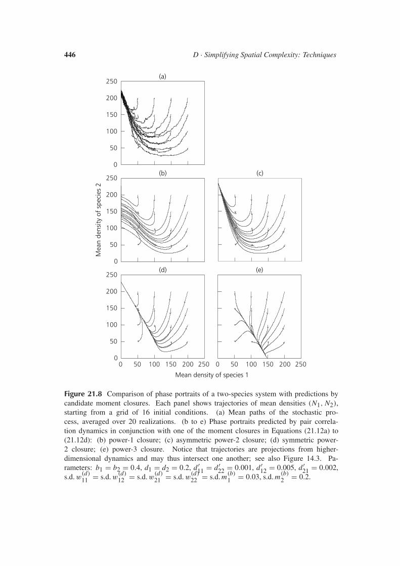
446 D · Simplifying Spatial Complexity: Techniques
(b) (c)250
200
150
100
50
(d)250
200
150
100
50
0 25020015010050
(a)
Mean density of species 1
(e)
0 25020015010050
Mea
n de
nsity
of
spec
ies
2
250
200
150
100
50
0
0
0
Figure 21.8 Comparison of phase portraits of a two-species system with predictions bycandidate moment closures. Each panel shows trajectories of mean densities (N1, N2),starting from a grid of 16 initial conditions. (a) Mean paths of the stochastic pro-cess, averaged over 20 realizations. (b to e) Phase portraits predicted by pair correla-tion dynamics in conjunction with one of the moment closures in Equations (21.12a) to(21.12d): (b) power-1 closure; (c) asymmetric power-2 closure; (d) symmetric power-2 closure; (e) power-3 closure. Notice that trajectories are projections from higher-dimensional dynamics and may thus intersect one another; see also Figure 14.3. Pa-rameters: b1 = b2 = 0.4, d1 = d2 = 0.2, d ′11 = d ′22 = 0.001, d ′12 = 0.005, d ′21 = 0.002,s.d. w(d)
11 = s.d. w(d)12 = s.d. w(d)
21 = s.d. w(d)22 = s.d. m(b)
1 = 0.03, s.d. m(b)2 = 0.2.

21 · Relaxation Projections and the Method of Moments 447
portraits of the actual dynamics. In particular, only the asymmetric power-2 closure captures the fine details of the phase portrait. Performance of thepower-1 closure is compromised by an instability at small densities, and thepower-3 closure even results in prediction of a wrong attractor.
The first test above (summarized in Figure 21.6) is independent of thecorrelation dynamics and therefore directly probes the accuracy of themoment closures. In contrast, the last two tests (recorded in Figures 21.7and 21.8) rely on evaluations of the joint performance of closures and cor-relation dynamics. While a benefit of the first test is its independence ofadditional theory, more discriminating results and more direct relevance topredictive quality are advantages of the latter pair. On the basis of thesetests, we have chosen the asymmetric power-2 closure for exploring eco-logical processes in Chapter 14. There is, however, much to be learnedabout moment closures, and we do not intend to suggest that this particu-lar closure performs best under all circumstances. To gain further insight,there appears to be no alternative to empirical tests for particular ecologicalsettings, in the manner of Figures 21.7 and 21.8.
21.5 Further Developments and ExtensionsIn this chapter we have derived a closed dynamical system for describingspatially heterogeneous change in general ecological communities of inter-acting species. Instead of considering the simultaneous dynamics of meanand pair densities, Equations (21.9) and (21.10), we can further simplifythe description by using Equation (21.10) alone. This is possible becauseCondition (C2), see Section 21.4, which is satisfied for small-scale spatialpatterns, implies lim|ξ |→∞ Cii (ξ) = N 2
i : consequently, information aboutmean densities is implicit in the description of pair dynamics. After insert-ing one of the moment closures from Equations (21.12), Equation (21.10)represents the central result of this chapter and provides a powerful tool forreducing the complexity of individual-based models. We have explainedhow this result is based on the method of moments: expressing the essen-tial degrees of freedom for a developing spatial pattern in terms of spa-tial moments and truncating the resulting moment hierarchy using a suit-able moment closure yields an approximation for the expected dynamicsof moments. The utility of such moment dynamics for describing and un-derstanding ecological processes under spatial heterogeneity is examinedin Section 21.4; a variety of successful applications are also presented inChapter 14.
448 D · Simplifying Spatial Complexity: Techniques
To conclude this chapter, we briefly review several directions for furtherelaborations on the method of moments. These extensions remove someremaining restrictions of the results presented and broaden the scope ofecological systems amenable to simplifying spatial complexity.
External heterogeneity and internal states
Moment dynamics can account for small-scale spatial heterogeneity in theexternal environment of populations. As discussed in Section 4.3, whichvariables are considered external to a system depends on how the system’sboundaries are defined. On a short time scale, for example, the concen-tration of soil nutrients in a spatially extended plant community may befixed in time and thus can be considered external to the system. In the longrun, however, we expect feedback between the dynamics of plants and nu-trients. Another example is the effect that landscape patterns have on thedispersal behavior of animals. Some butterflies, for instance, inhabit mead-ows that arise in gaps created by forest fires, and while the meadows areeasily traversed, stretches of forest act as dispersal barriers. In this case,there is no significant feedback between the dynamics of butterflies andforest trees. With or without such feedback, spatial heterogeneity of en-vironmental conditions encountered by a focal population can be formallytreated on par with the heterogeneity arising from the presence of extrapopulations. Straightforward generalizations of Equations (21.10) there-fore account for a population’s unfolding against the backdrop of a hetero-geneous landscape. Salient state variables are the auto-correlations of thefocal population, complemented by the auto-correlations of environmentalconditions (these may be variable or fixed) as well as the cross-correlationsbetween the population and its environment. Moment dynamics of thiskind can provide insights into complex interactions between internal andexternal mechanisms of ecological pattern formation.
Another extension of moment dynamics allows the incorporation of de-tails about the state of individuals. For example, instead of characterizinga population of trees just by the locations on which they are centered, thesize of each tree (height or crown diameter) can be accounted for as well.Implications of asymmetric competition for light, for instance, can thusbe studied in spatially heterogeneous settings. Also, a plea for dynamicneighborhoods (see Section 2.5) that vary with, for example, plant size canbe met in this way. Other such internal states by which location-basedinformation can be augmented are the age of individuals, their physiologi-cal status, or their phenotype. In each case, pair correlation densities take

21 · Relaxation Projections and the Method of Moments 449
two extra arguments, measuring the internal state of paired individuals inaddition to their distance. Merging physiologically structured and spatiallystructured population models in such a way is not easy; yet, such integrationwould bring models closer to the reality of field systems and is therefore animportant path to follow in developing ecological theory.
Fluctuation and correlation corrections
The importance of taking an “individual’s-eye view” in determining the re-sponse of a population to its environment has already been emphasized. Inthis context, we must realize that, for populations of finite density, anybounded neighborhood around an individual will comprise only a finitenumber of individuals. When numbers of neighbors are large, resultingsampling variation is negligible. But for many systems, neighbors aroundeach individual are few enough for the latter to experience substantiallyvarying local environments. We thus have to ask whether and how suchfluctuations feed through to population dynamics and their description bymoment equations. The answer comes in three steps.
We observe, first, that local fluctuations do not bear on the expecteddynamics of moments if individuals respond linearly to the local densi-ties of individuals in their surroundings. Equations (21.1a) and (21.1c) arebased on this assumption – per capita birth and death rates in these spa-tial analogues of Lotka–Volterra competition depend linearly on the patternof individuals – and therefore no fluctuation-related terms arise in Equa-tions (21.9) or (21.10). Under such circumstances, the mean response of apopulation to a distribution of environments equals the response predictedfor the distribution mean; consequently, local fluctuations have no effect.
Second, even in the absence of spatial structure (i.e., without pair corre-lations), the behavior of a well-mixed population of individuals that respondnonlinearly to relatively small numbers of neighbors is different from thatof a population under mean-field conditions. A typical result is explainedin Box 21.5.
Third, we can investigate the implications of nonlinear responses ofindividuals to local fluctuations in the presence of pair correlations.Let us consider a single species for which per capita birth and deathrates are nonlinearly dependent on local densities, so that, analogousto Equations (21.1a) and (21.1c), we have D(x, p) = d (n(x, p)) andB(x, x ′, p) = b (n(x, p)) m(b)(x ′ − x), with local densities n(x, p) =∫
w(x ′′ − x)[p(x ′′)− δx(x ′′)]dx ′′. Under mean-field conditions, the globalmean density simply changes according to d
dt N = f (N )N , with a per
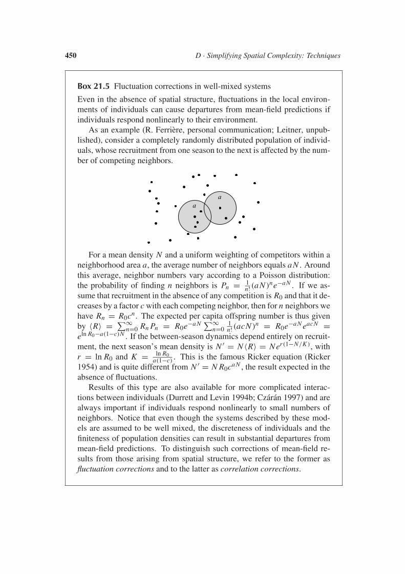
450 D · Simplifying Spatial Complexity: Techniques
Box 21.5 Fluctuation corrections in well-mixed systems
Even in the absence of spatial structure, fluctuations in the local environ-ments of individuals can cause departures from mean-field predictions ifindividuals respond nonlinearly to their environment.
As an example (R. Ferriere, personal communication; Leitner, unpub-lished), consider a completely randomly distributed population of individ-uals, whose recruitment from one season to the next is affected by the num-ber of competing neighbors.
aa
For a mean density N and a uniform weighting of competitors within aneighborhood area a, the average number of neighbors equals aN . Aroundthis average, neighbor numbers vary according to a Poisson distribution:the probability of finding n neighbors is Pn = 1
n! (aN )ne−aN . If we as-sume that recruitment in the absence of any competition is R0 and that it de-creases by a factor c with each competing neighbor, then for n neighbors wehave Rn = R0cn . The expected per capita offspring number is thus givenby 〈R〉 = ∑∞
n=0 Rn Pn = R0e−aN ∑∞n=0
1n! (acN )n = R0e−aN eacN =
eln R0−a(1−c)N . If the between-season dynamics depend entirely on recruit-ment, the next season’s mean density is N ′ = N 〈R〉 = Ner(1−N/K ), withr = ln R0 and K = ln R0
a(1−c) . This is the famous Ricker equation (Ricker1954) and is quite different from N ′ = N R0caN , the result expected in theabsence of fluctuations.
Results of this type are also available for more complicated interac-tions between individuals (Durrett and Levin 1994b; Czaran 1997) and arealways important if individuals respond nonlinearly to small numbers ofneighbors. Notice that even though the systems described by these mod-els are assumed to be well mixed, the discreteness of individuals and thefiniteness of population densities can result in substantial departures frommean-field predictions. To distinguish such corrections of mean-field re-sults from those arising from spatial structure, we refer to the former asfluctuation corrections and to the latter as correlation corrections.

21 · Relaxation Projections and the Method of Moments 451
capita growth rate f = b − d . With local fluctuations and correlations,however, reasoning analogous to that in Section 21.3 shows that the mean-field result ought to be replaced with d
dt N = [ f (n) + 12σ
2 f ′′(n)]N , withan average n = N−1
∫w(ξ)C(ξ)dξ and a variance σ 2 of local densities.
Comparing both dynamics for the global mean density, we observe twocorrections relative to the mean-field result. First, a correlation correc-tion replaces the global mean density N with the average local density nin the argument of the response function f . This reflects the fact that, inthe presence of correlations, the average environment around individuals isdifferent from the environment averaged over the entire habitat. Withoutpair correlations, we have C(ξ) = N 2 [see Equation (21.11)], which yieldsn = N , thus recovering the mean-field result. Second, a fluctuation correc-tion adds the extra term 1
2σ2 f ′′(n) to the population’s response function.
Notice that the sign of the term and thus the direction of this correction de-pends on the response function’s curvature at the average local density. Wealso see that this term vanishes if there are no fluctuations in local densities(σ 2 = 0) or if the response function is linear ( f ′′ = 0).
Other spatial statistics and further reductions of complexity
Low-order correlation densities often capture the essential degrees of free-dom in spatial ecological processes. For isotropic systems, spatial com-plexity can be simplified even further by considering angular averages ofpair densities, as explained in Section 21.3 and Figure 21.2. Such a trans-formation of Equation (21.10) then describes pair densities as a functionof radial distance instead of vectorial distance. One further step in remov-ing non-essential degrees of freedom can be accomplished by a short-rangeexpansion of Equation (21.10), approximating pair dynamics by the dy-namics of intercept, slope, and curvature of pair densities at distance zero.That slope in particular is often a good measure of a pattern’s correlationlength, characterizing how rapidly pair correlations decay with distance.Correlation lengths can change in the course of ecological dynamics andthus carry key information about patterns as well as processes.
These extensions emphasize that alternative kinds of spatial statisticsmay be most appropriate for describing a given ecological system. In fact,correlation functions are not the only choice of statistics suitable for sim-plifying spatial complexity – for particular systems, other relaxation pro-jections may offer superior performance. Chapter 15 provides an exampleby constructing a patch-based approximation of a spatial host–parasite sys-tem. Instead of tracing through time the probabilistic cellular-automaton

452 D · Simplifying Spatial Complexity: Techniques
dynamics of that system, only the expected average abundances of speciesin patches of different types are considered, thus yielding a deterministicdescription of substantially reduced complexity. Other examples are the so-called local structure approximations of Hiebeler (1997) and the pair-edgeapproximation of Ellner et al. (1998). The latter approach is especiallysuited to a class of large-scale spatial patterns where two types of popu-lations live in adjacent domains and a traveling invasion wave develops attheir interface (see also Chapters 16, 17, 22, and 23); for such patterns, theposition of the invasion front is the central degree of freedom.
This chapter has introduced a general theory of small-scale heterogene-ity in ecological processes that is based on correlation densities. Eventu-ally, a tool kit of successful relaxation projections and associated spatialstatistics should become available to help ecologists reduce various kindsof complex spatio-temporal models to manageable approximations.
Appendix 21.A Derivation of Pair DynamicsIn this appendix we explain how to derive the dynamics of corrected pair densities,presented in Equation (21.10).
The expected rates of change in corrected pair densities Ci j (ξ) are determinedby the first jump moments of these densities, see Equation (21.6c),
d
dtCi j (ξ) =
∫ai j (ξ, p)P(p) dp , (21.13a)
with contributions coming from birth, death, and movement events,
ai j (ξ, p) = a(b)i j (ξ, p)+ a(d)
i j (ξ, p)+ a(m)i j (ξ, p) . (21.13b)
Let us focus on the birth contribution first. From Equation (21.6c) and Equa-tion (21.2b), we have
a(b)i j (ξ, p) =
∫ [Ci j (ξ, p′)− Ci j (ξ, p)
]×∑
k
∫∫Bk(x, x ′, p)pk(x)�(p + ukδx ′ − p′) dxdx ′dp′ ,
(21.14a)
which, after collapsing the integration over p′ using the definition of the general-ized delta function (see Box 21.4), simplifies to
a(b)i j (ξ, p) =
∑k
∫∫ [Ci j (ξ, p + ukδx ′)− Ci j (ξ, p)
]× Bk(x, x ′, p)pk(x) dxdx ′ .
(21.14b)

21 · Relaxation Projections and the Method of Moments 453
With Ci j (ξ, p + ukδx ′) = 1A
∫(p + ukδx ′)i (x)[(p + ukδx ′)j (x + ξ) − δi jδx (x +
ξ)] dx = 1A
∫ [pi (x) + δikδx ′(x)][pj (x + ξ) + δjkδx ′(x + ξ) − δi jδ(ξ)] dx =Ci j (ξ, p)+ 1
A [δjk pi (x ′−ξ)+δik pj (x ′+ξ)+δikδjkδ(ξ)−δikδi jδ(ξ)] = Ci j (ξ, p)+1A [δjk pi (x ′ − ξ)+ δik pj (x ′ + ξ)], we obtain
a(b)i j (ξ, p) ==∑
k
1
A
∫∫ [δjk pi (x ′−ξ)+δik pj (x ′+ξ)
]Bk(x,x ′,p)pk(x)dxdx ′
= 1
A
∫∫ [pi (x ′−ξ)Bj (x,x ′,p)pj (x)+ pj (x ′ + ξ)Bi (x,x ′,p)pi (x)
]dxdx ′
= 1
A
∫∫pi (x)pj (x ′+ξ)Bi (x,x ′,p)dxdx ′+〈i, j,ξ → j,i,−ξ〉 . (21.14c)
As in Equation (21.10), the expression 〈i, j, ξ → j, i,−ξ〉 is shorthand and standsfor all its preceding terms after changing i to j , j to i , and ξ to −ξ . Inserting Bi
according to Equation (21.1c) yields
a(b)i j (ξ,p) = 1
A
∫∫pi (x)pj (x ′+ ξ)
[bi +
∑k
b′ik
∫w
(b)ik (x ′′ − x)
× [pk(x ′′)− δikδx (x ′′)]dx ′′]m(b)
i (x ′− x)dxdx ′+ 〈i, j,ξ → j,i,−ξ〉 ,
(21.14d)
or, when separating terms for density-independent and density-dependent birth,
a(b)i j (ξ, p) = + bi
1
A
∫∫pi (x)pj (x ′ + ξ)m(b)
i (x ′ − x) dxdx ′
+∑
k
b′ik1
A
∫∫∫pi (x)pj (x ′ + ξ)
× [pk(x ′′)− δikδx (x ′′)]
m(b)i (x ′ − x)w
(b)ik (x ′′ − x) dxdx ′dx ′′
+ 〈i, j, ξ → j, i,−ξ〉 .
(21.14e)
The x-integration of pi pj in the first term and of pi pj pk in the second resemblesthe definitions of Ci j and Ti jk in Equation (21.4a) and (21.4b), respectively. Forfull compatibility with integrands in these definitions, we must subtract (and thenadd in again) one self-pair term for Ci j , pi (x)pj (x ′ + ξ) = pi (x)[pj (x ′ + ξ) −δi jδx (x ′ + ξ)] + pi (x)δi jδx (x ′ + ξ), and two such terms for Ti jk , pi (x)pj (x ′ +ξ)[pk(x ′′)− δikδx (x ′′)] = pi (x)[pj (x ′ + ξ)− δi jδx (x ′ + ξ)][pk(x ′′)− δikδx (x ′′)−δjkδx ′+ξ (x ′′)] + pi (x)δi jδx (x ′ + ξ)[pk(x ′′)− δjkδx ′+ξ (x ′′)] + pi (x)[pj (x ′ + ξ)−δi jδx (x ′ + ξ)]δjkδx ′+ξ (x ′′). With ξ ′ = x ′ − x and ξ ′′ = x ′′ − x , we thus obtain

454 D · Simplifying Spatial Complexity: Techniques
a(b)i j (ξ, p) =+ bi
∫m(b)
i (ξ ′)Ci j (ξ + ξ ′, p) dξ ′
+ δi j bi m(b)i (−ξ)Ni (p)
+∑
k
b′ik
∫∫m(b)
i (ξ ′)w(b)ik (ξ ′′)Ti jk(ξ + ξ ′, ξ ′′, p) dξ ′dξ ′′
+ δi j m(b)i (−ξ)
∑k
b′ik
∫w
(b)ik (ξ ′′)Cik(ξ
′′, p) dξ ′′
+ b′i j
∫m(b)
i (ξ ′)w(b)i j (ξ + ξ ′)Ci j (ξ + ξ ′, p) dξ ′
+ 〈i, j, ξ → j, i,−ξ〉 .
(21.14f)
We now turn to calculating the death contribution,
a(d)i j (ξ, p) =
∑k
∫ [Ci j (ξ, p − ukδx )− Ci j (ξ, p)
]Dk(x, p)pk(x) dx . (21.15a)
With Ci j (ξ, p − ukδx ) = 1A
∫ [pi (x ′) − δikδx (x ′)][pj (x ′ + ξ) − δjkδx (x ′ + ξ) −δi jδ(ξ)] dx ′ = Ci j (ξ, p) + 1
A [−δjk pi (x − ξ) − δik pj (x + ξ) + δikδjkδ(ξ) +δikδi jδ(ξ)] = Ci j (ξ, p)− 1
A {δik[pj (x+ ξ)− δjkδ(ξ)]+ δjk [pi (x− ξ)− δikδ(ξ)]},we obtain
a(d)i j (ξ, p) =− 1
A
∫pi (x)
[pj (x + ξ)− δi jδ(ξ)
]Di (x, p) dx
+ 〈i, j, ξ → j, i,−ξ〉 .
(21.15b)
After inserting Di according to Equation (21.1a), this yields
a(d)i j (ξ, p) =− di
1
A
∫pi (x)
[pj (x + ξ)− δi jδ(ξ)
]dx
−∑
k
d ′ik1
A
∫∫pi (x)
[pj (x + ξ)− δi jδ(ξ)
]× [pk(x ′′)− δikδx (x ′′)
]w
(d)ik (x ′′ − x) dxdx ′′
+ 〈i, j, ξ → j, i,−ξ〉 .
(21.15c)
Notice that the integral in the first term matches the definition of Ci j . To achievefull compatibility with the definition of Ti jk in the second term, we subtract (andthen add in again) a self-pair term, as we did in calculating the birth contribu-tion: pi (x)[pj (x + ξ) − δi jδ(ξ)][pk(x ′′) − δikδx (x ′′)] = pi (x)[pj (x + ξ) −δi jδx (x + ξ)][pk(x ′′)− δikδx (x ′′)− δjkδx+ξ (x ′′)] + pi (x)[pj (x + ξ)− δi jδx (x +ξ)]δjkδx+ξ (x ′′). With ξ ′′ = x ′′ − x , we arrive at
a(d)i j (ξ, p) =− di Ci j (ξ, p)
−∑
k
d ′ik
∫w
(d)ik (ξ ′′)Ti jk(ξ, ξ ′′, p) dξ ′′
− d ′i jw(d)i j (ξ)Ci j (ξ, p)
+ 〈i, j, ξ → j, i,−ξ〉 .
(21.15d)

21 · Relaxation Projections and the Method of Moments 455
Finally, we calculate the contribution of movement events to the dynamics ofcorrected pair densities,
a(m)i j (ξ, p) =
∑k
∫∫ [Ci j (ξ, p − ukδx + ukδx ′)− Ci j (ξ, p)
]× Mk(x, x ′, p)pk(x) dxdx ′ .
(21.16a)
With Ci j (ξ, p − ukδx + ukδx ′) = 1A
∫ [pi (x ′′)− δikδx (x ′′)+ δikδx ′(x ′′)][pj (x ′′ +ξ)−δjkδx (x ′′+ξ)+δjkδx ′(x ′′+ξ)−δi jδ(ξ)] dx ′′ = Ci j (ξ, p)+ 1
A [−δjk pi (x−ξ)+δjk pi (x ′−ξ)−δik pj (x+ξ)+δikδjkδ(ξ)−δikδjkδx ′(x+ξ)+δikδi jδ(ξ)+δik pj (x ′+ξ)− δikδjkδx (x ′ + ξ)+ δikδjkδ(ξ)− δikδi jδ(ξ)] = Ci j (ξ, p)− 1
A {δik[pj (x ′ + ξ)−pj (x + ξ)− δjkδx (x ′ + ξ)+ δjkδ(ξ)] + δjk [pi (x ′ − ξ)− pi (x − ξ)− δikδx (x ′ −ξ)+ δikδ(ξ)]}, and with Mi (x, x ′, p) = mi (x ′ − x) from Equation (21.1b), we get
a(m)i j (ξ, p) = + 1
A
∫∫pi (x)
[pj (x ′ + ξ)− pj (x + ξ)
− δi jδx (x ′ + ξ)+ δi jδ(ξ)]mi (x ′ − x) dxdx ′
+ 〈i, j, ξ → j, i,−ξ〉 .
(21.16b)
For matching the definition of Ci j , we rewrite this equation by splitting the integralin two,
a(m)i j (ξ, p) =+ 1
A
∫∫pi (x)
[pj (x ′ + ξ)− δi jδx (x ′ + ξ)
]mi (x ′ − x) dxdx ′
− 1
A
∫∫pi (x)
[pj (x + ξ)− δi jδ(ξ)
]mi (x ′ − x) dxdx ′
+ 〈i, j, ξ → j, i,−ξ〉 .
(21.16c)
With ξ ′ = x ′ − x , this yields
a(m)i j (ξ, p) =+
∫mi (ξ
′)Ci j (ξ + ξ ′, p) dξ ′
− Ci j (ξ, p)
∫mi (ξ
′) dξ ′
+ 〈i, j, ξ → j, i,−ξ〉 .
(21.16d)
Inserting the three results from Equations (21.14f), (21.15d), and (21.16d)into Equations (21.13) recovers the dynamics of corrected pair densities,Equation (21.10).

ReferencesReferences in the book in which this chapter is published are integrated in a single list,which appears on pp. 517–552. For the purpose of this reprint, references cited in thechapter have been assembled below.
Anderson RM & May RM (1991). Infectious Diseases of Humans: Dynamics andControl. Oxford, UK: Oxford University Press
Bailey NTJ (1975). The Mathematical Theory of Infectious Diseases and Its Ap-plications. London, UK: Griffin
Bolker B & Pacala SW (1997). Using moment equations to understand stochasti-cally driven spatial pattern formation in ecological systems. Theoretical Popu-lation Biology 52:179–197
Dieckmann U (1994). Coevolutionary Dynamics of Stochastic Replicator Systems.Juelich, Germany: Central Library of the Research Center Juelich
Dieckmann U, Herben T & Law R (1997). Spatio-temporal processes in plantcommunities. In Yearbook 1995/96, Institute for Advanced Study Berlin, ed.Lepenies W, pp. 296–326. Berlin, Germany: Nicolaische Verlagsbuchhand-lung
Dieckmann U, Herben T & Law R. Spatio-temporal processes in ecological com-munities. CWI Quarterly. In press
Diggle PJ (1983). Statistical Analysis of Spatial Point Patterns. London, UK:Academic Press
Dirac PAM (1926). The physical interpretation of the quantum dynamics. Pro-ceedings of the Royal Society of London A 113:621–641
Dirac PAM (1958). The Principles of Quantum Dynamics, 4th edn. Oxford, UK:Clarendon Press
Ellner SP, Sasaki A, Haraguchi Y & Matsuda H (1998). Speed of invasion inlattice population models: Pair-edge approximation. Journal of MathematicalBiology 36(5):469–484
Hiebeler D (1997). Stochastic spatial models: From simulations to mean field andlocal structure approximations. Journal of Theoretical Biology 187:307–319
Hogeweg P (1988). Cellular automata as a paradigm for ecological modeling.Applied Mathematics and Computation 27:81–100
Holsinger KE & Roughgarden J (1985). A model for the dynamics of an annualplant-population. Theoretical Population Biology 28:288–313
Jammer M (1966). The Conceptual Development of Quantum Mechanics. NewYork, NY, USA: McGraw-Hill
Kirkwood JG (1935). Statistical mechanics of fluid mixtures. Journal of ChemicalPhysics 3:300–313
Leitner W. From individual life history processes to population dynamics: a deriva-tion of the Ricker map. Unpublished
Levin SA (1974). Dispersion and population interactions. The American Natural-ist 108:207–228
Levin SA (1976). Population dynamical models in heterogeneous environments.Annual Review of Ecology and Systematics, Vol. 7, pp. 287–310

Lewontin RC (1974). The Genetic Basis of Evolutionary Change. New York,NY, USA: Columbia University Press
Mahdi A & Law R (1987). On the spatial organization of plant species in a lime-stone grassland community. Journal of Ecology 75:459–476
Pacala SW (1986). Neighborhood models of plant population dynamics. II. Multi-species models of annuals. Theoretical Population Biology 29:262–292
Pacala SW & Silander JA Jr (1985). Neighborhood models of plant popula-tion dynamics. I. Single-species models of annuals. The American Naturalist125:385–411
Ricker WE (1954). Stock and recruitment. Journal of the Fisheries ResearchBoard of Canada 11: 559–623
Ripley BD (1981). Spatial Statistics. New York, NY, USA: WileySchwartz L (1950). Theorie des distributions. Paris, France: HermannTurkington RA & Harper JL (1979). The growth, distribution and neighbour rela-
tionships of Trifolium repens in a permanent pasture. I. Ordination, pattern andcontact. Journal of Ecology 67:201–218
Turkington RA & Harper JL (1979). The growth, distribution and neighbour rela-tionships of Trifolium repens in a permanent pasture. I. Ordination, pattern andcontact. Journal of Ecology 67:201–218
van Kampen NG (1992). Stochastic Processes in Physics and Chemistry. Amster-dam, Netherlands: North-Holland
Watt AS (1947). Pattern and process in the plant community. Journal of Ecology35:1–22
Weinberger HF (1982). Long-time behaviour of a class of biological models.SIAM Journal of Mathematical Analysis 13:353–396
Weiner J (1982). A neighborhood model of annual-plant interference. Ecology63:1237–1241
Weiner J & Conte PT (1981). Dispersal and neighborhood effects in an annualplant competition model. Ecological Modelling 13:131–147
Ziman JM (1979). Models of Disorder: The Theoretical Physics of Homoge-neously Disordered Systems. Cambridge, UK: Cambridge University Press