relaxation of rank-1 spatial constraint in overdetermined blind source separation

Daichi KitamuraNobutaka Ono

Hiroshi SawadaHirokazu KameokaHiroshi Saruwatari

Relaxation of Rank-1 Spatial Constraint in Overdetermined Blind Source Separation

(SOKENDAI)(NII/SOKENDAI)(NTT)(The Univ. of Tokyo/NTT)(The Univ. of Tokyo)

EUSIPCO 2015, 2 Sept.,14:30 - 16:10, SS30 Acoustic scene analysis using microphone array

Research Background• Blind source separation (BSS)

– Estimation of original sources from the mixture signal

– We only focus on overdetermined situations • Number of sources Number of microphones• Ex) Independent component analysis, independent vector analysis

• Applications of BSS– Acoustic scene analysis, speech enhancement, music

analysis, reproduction of sound field, etc.2/21

Original sources Observation (mixture) Estimated sources

Mixing system BSS

Unknown

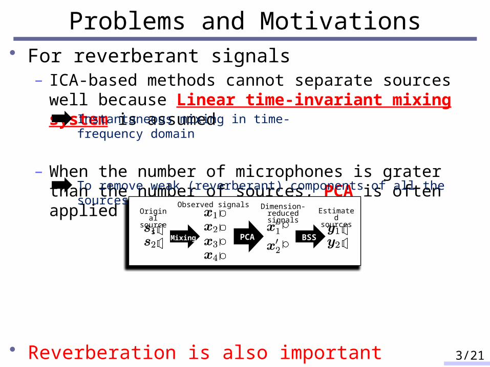
Problems and Motivations• For reverberant signals

– ICA-based methods cannot separate sources well because Linear time-invariant mixing system is assumed

– When the number of microphones is grater than the number of sources, PCA is often applied before BSS

• Reverberation is also important information to analyze acoustic scenes– We should separate the sources with their own

reverberations.3/21

Original sources

Observed signals

Mixing

Estimated sources

BSS

Dimension-reduced signals

PCA

Instantaneous mixing in time-frequency domain

To remove weak (reverberant) components of all the sources

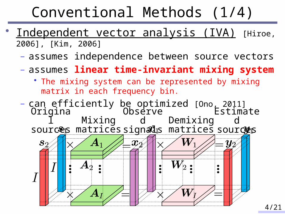
• Independent vector analysis (IVA) [Hiroe, 2006], [Kim, 2006]

– assumes independence between source vectors – assumes linear time-invariant mixing system

• The mixing system can be represented by mixing matrix in each frequency bin.

– can efficiently be optimized [Ono, 2011]

Conventional Methods (1/4)

4/21

……

Original sources Mixing

matrices…… …

Observed signals Demixing

matrices

Estimated sources

Conventional Methods (2/4)• Nonnegative matrix factorization (NMF) [Lee, 2001]

– decomposes spectrogram into spectral bases

– Decomposed bases should be clustered into each source.• Very difficult problem

– Multichannel extension of NMF has been proposed.

5/21

Amplitude

Am

plitu

de

Observed matrix(power spectrogram)

Basis matrix(spectral patterns)

Activation matrix(Time-varying gain)

Time

: Number of frequency bins : Number of time frames : Number of bases

Time

Freq

uenc

y

Freq

uenc

y

Basis

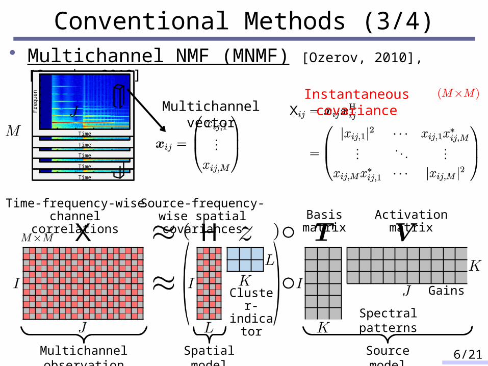
• Multichannel NMF (MNMF) [Ozerov, 2010], [Sawada, 2013]

　　　　　　　　　　　　　　　　　　　　　　　　　　　　　　　　　　　　　　　　　

　　　　　　　　　　　　　　　　　　　　　　　　　

　　　　　　　　　　　　　　　　　　　　　　　　　　　　　　　　　　　　　　　　　

　　　　　　　　　　　　　　　　　　　　　　　　　

　　　　　　　　　　　　　　　　　　　　　　　　　　　　　　　　　　　　　　

　　　　　　　　　　　　　　　　　　　　　　　　　

　　　　　　　　　　　　　　　　　　　　　　　　　　　　

　　　　　　　　　　　　　　　　　　　　　　　　　

　　　　　　　　　　　　　　　　　　　　　　　　　　　　

　　　　　　　　　　　　　　　　　　　　　　　　　

　　　　　　　　　　　　　　　　　　　　　　　　　　　　

　　　　　　　　　　　　　　　　　　　　　　　　　


6/21

Time-frequency-wise channel correlations

Multichannel observation

Multichannel vector

Time

Freque

nc

y

Time

Freque

nc

y

Time

Freque

nc

y

Time

Freque

nc

y

Time

Freque

nc

y

Instantaneous covariance

Source-frequency-wise spatial covariances Basis matrix Activation matrix

Spatial model Source model

Cluster-indicator Spectral patterns

Gains

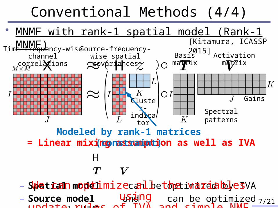
• MNMF with rank-1 spatial model (Rank-1 MNMF)

– Spatial model can be optimized by IVA– Source model and can be optimized by simple NMFWe can optimize all the variables using

update rules of IVA and simple NMF

　　　　　　　　　　　　　　　　　　　　　　　　　　　　　　　　　　　　　　　　　

　　　　　　　　　　　　　　　　　　　　　　　　　

　　　　　　　　　　　　　　　　　　　　　　　　　　　　　　　　　　　　　　　　　

　　　　　　　　　　　　　　　　　　　　　　　　　

　　　　　　　　　　　　　　　　　　　　　　　　　　　　　　　　　　　　　　

　　　　　　　　　　　　　　　　　　　　　　　　　

　　　　　　　　　　　　　　　　　　　　　　　　　　　　

　　　　　　　　　　　　　　　　　　　　　　　　　

　　　　　　　　　　　　　　　　　　　　　　　　　　　　

　　　　　　　　　　　　　　　　　　　　　　　　　

　　　　　　　　　　　　　　　　　　　　　　　　　　　　

　　　　　　　　　　　　　　　　　　　　　　　　　

Time-frequency-wise channel correlations

Source-frequency-wise spatial covariances Basis matrix Activation matrix

Spectral patterns

Gains


7/21

[Kitamura, ICASSP 2015]

= Linear mixing assumption as well as IVAModeled by rank-1 matrices (constraint)

Cluster-indicator

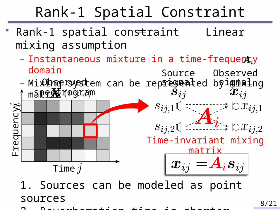
• Rank-1 spatial constraint Linear mixing assumption– Instantaneous mixture in a time-frequency domain– Mixing system can be represented by mixing matrix

Rank-1 Spatial Constraint

8/21

1. Sources can be modeled as point sources2. Reverberation time is shorter than FFT length

　　　　　　　　　　　　　　　　　　　　　　　　　　　　　　　　　　　Fr

eque

ncy

Time

Observed spectrogram

Time-invariant mixing matrix

Observed signal

Source signal

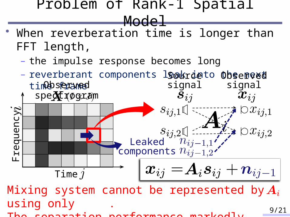
• When reverberation time is longer than FFT length,– the impulse response becomes long– reverberant components leak into the next time frame

Problem of Rank-1 Spatial Model

9/21

Mixing system cannot be represented by using only . The separation performance markedly degrades.

　　　　　　　　　　　　　　　　　　　　　　　　　　　　　　　　　　　Fr

eque

ncy

Time

Observed spectrogramObserved

signalSource signal

Leaked components

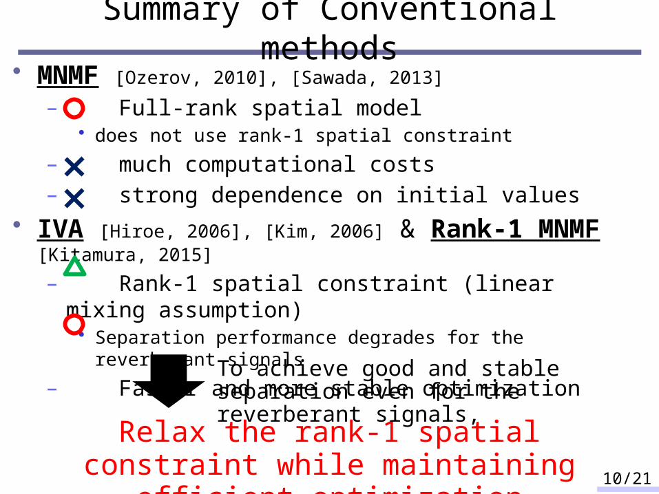
Summary of Conventional methods• MNMF [Ozerov, 2010], [Sawada, 2013]

– Full-rank spatial model• does not use rank-1 spatial constraint

– much computational costs– strong dependence on initial values

• IVA [Hiroe, 2006], [Kim, 2006] & Rank-1 MNMF [Kitamura, 2015]

– Rank-1 spatial constraint (linear mixing assumption)• Separation performance degrades for the reverberant signals

– Faster and more stable optimization

10/21

Relax the rank-1 spatial constraint while maintaining efficient optimization

To achieve good and stable separation even for the reverberant signals,

• Dimensionality reduction with principal component analysis (PCA)– remove reverberant components of all the sources by PCA– But the reverberant components are important!

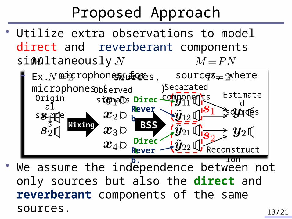
• Utilize extra observations to model direct and reverberant components simultaneously.– microphones for sources, where

Proposed Approach

11/21

Original sources

Observed signals

Mixing

Estimated sources

BSS

Dimension-reduced signals

PCA

Ex. sources, microphones ( )

Proposed Approach

12/21


Original sources

Observed signals

Mixing


Estimated sources

Reconstruction

Separated components

BSS

IVA or Rank-1 MNMF

Proposed Approach

13/21


Original sources

Observed signals

Mixing


DirectReverb.

DirectReverb.

Estimated sources

Reconstruction


BSS

• We assume the independence between not only sources but also the direct and reverberant components of the same sources.

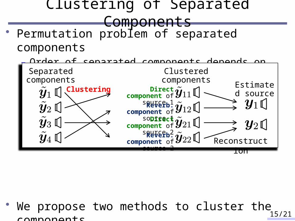
• Permutation problem of separated components– Order of separated components depends on initial values

• We propose two methods to cluster the components– 1. Using cross-correlations for IVA– 2. Sharing basis matrices for Rank-1 MNMF

Clustering of Separated Components

14/21


? Which separated components belong to which source?

• Permutation problem of separated components– Order of separated components depends on initial values

• We propose two methods to cluster the components– 1. Using cross-correlations for IVA– 2. Sharing basis matrices for Rank-1 MNMF

Clustering of Separated Components

15/21

Estimated source

Reconstruction


Clustered components

Direct component of source 1

Clustering

Reverb. component of source 1



Clustering Using Spectrogram Correlation• Direct and reverberant components of the same

source have a strong cross-correlation.

• Cross-correlation of two power spectrograms

– Calculate for all combination of separated components– Merge the components in a descending order of

16/21

Power spectrogram of Power spectrogram of

・・・

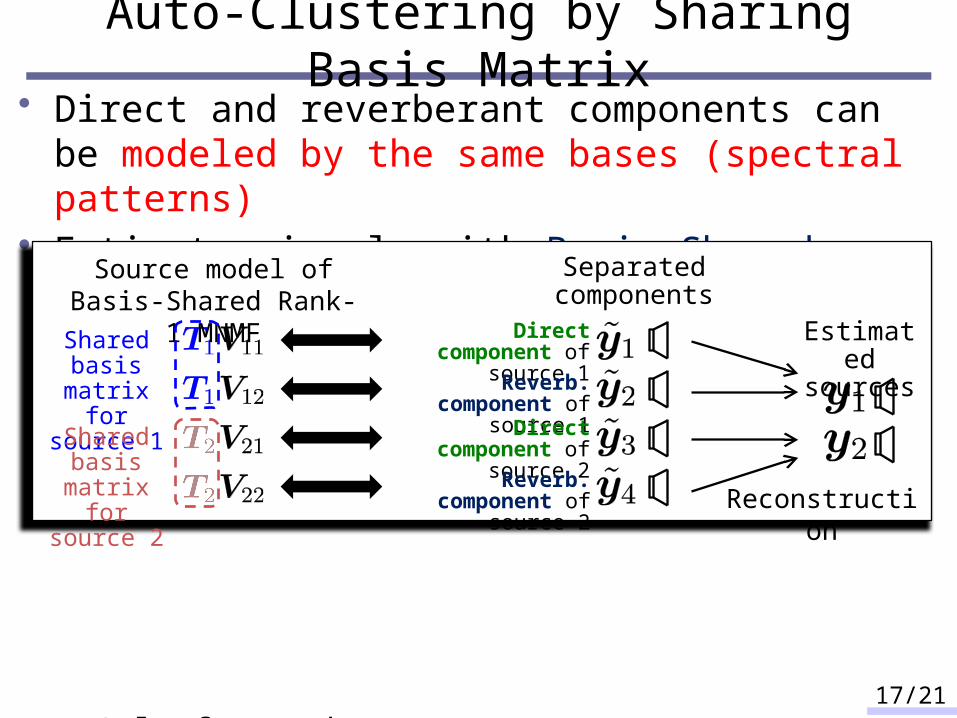
• Direct and reverberant components can be modeled by the same bases (spectral patterns)

• Estimate signals with Basis-Shared Rank-1 MNMF

– Only for Rank-1 MNMF• because IVA doesn’t have NMF source model

– By imposing basis-shared source model, Rank-1 MNMF can automatically cluster the components.

Auto-Clustering by Sharing Basis Matrix

17/21


Source model of Basis-Shared Rank-1 MNMF

Shared basis matrix for source 1

Reconstruction

Estimated sources

Shared basis matrix for source 2





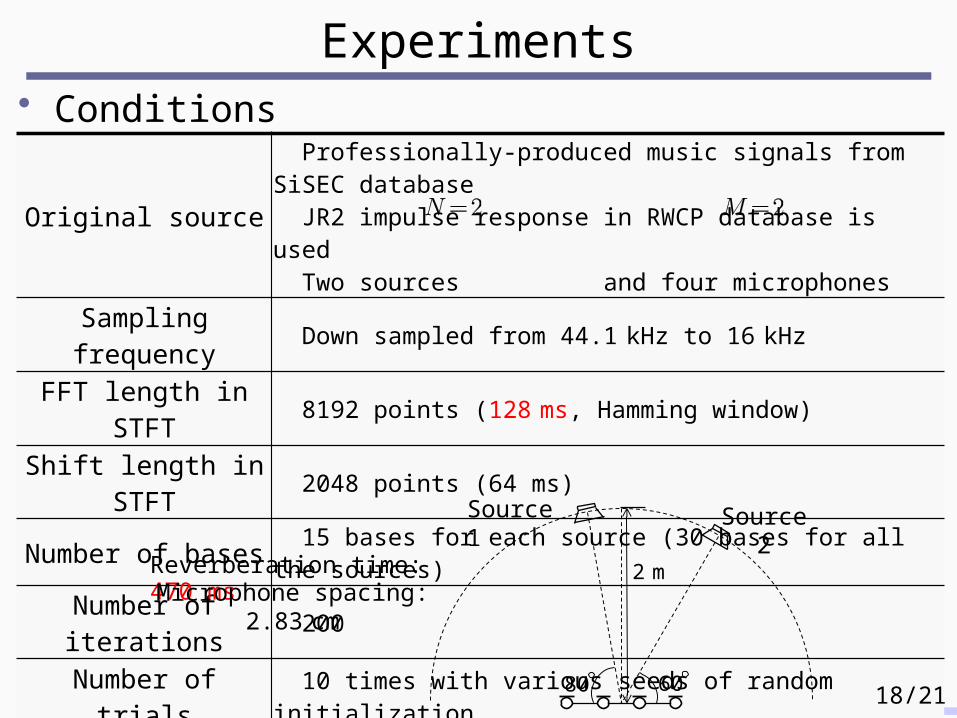
• Conditions

– JR2 impulse response

Experiments

Original source Professionally-produced music signals from SiSEC database JR2 impulse response in RWCP database is used Two sources and four microphones

Sampling frequency Down sampled from 44.1 kHz to 16 kHz

FFT length in STFT 8192 points (128 ms, Hamming window)

Shift length in STFT 2048 points (64 ms)

Number of bases 15 bases for each source (30 bases for all the sources)

Number of iterations 200

Number of trials 10 times with various seeds of random initialization

Evaluation criterion Average SDR improvement and its deviation

18/21

Reverberation time: 470 ms 2 m

Source 1

80 60

Microphone spacing: 2.83 cm

Source 2

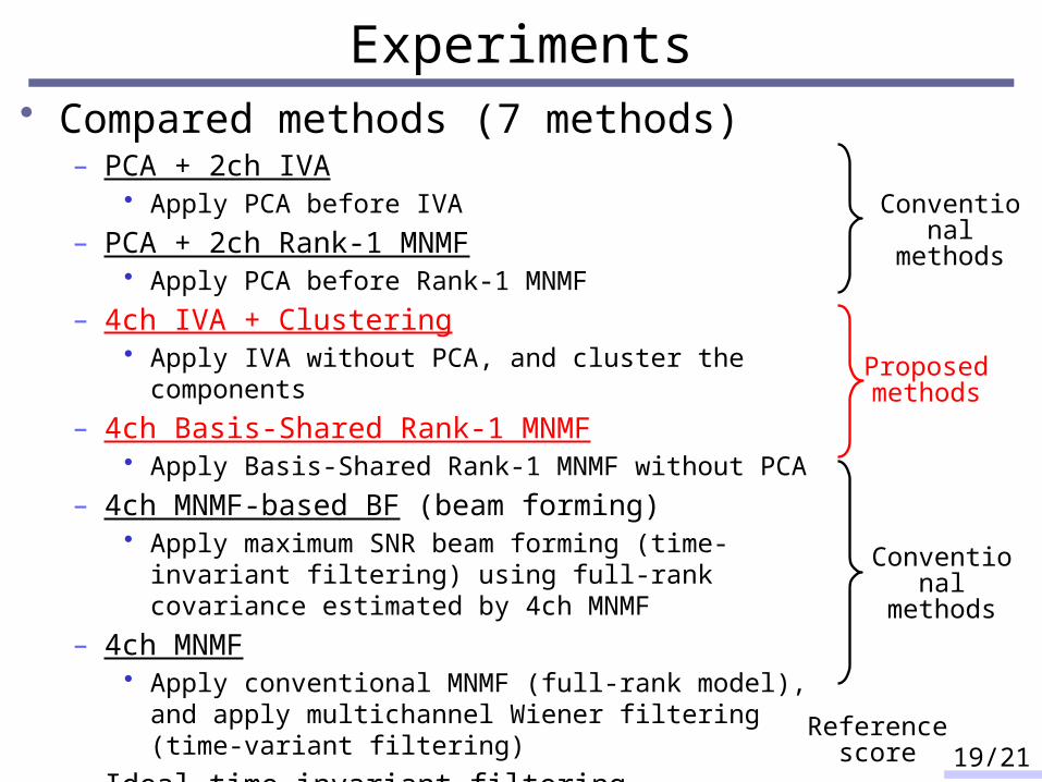
• Compared methods (7 methods)– PCA + 2ch IVA

• Apply PCA before IVA– PCA + 2ch Rank-1 MNMF

• Apply PCA before Rank-1 MNMF– 4ch IVA + Clustering

• Apply IVA without PCA, and cluster the components– 4ch Basis-Shared Rank-1 MNMF

• Apply Basis-Shared Rank-1 MNMF without PCA– 4ch MNMF-based BF (beam forming)

• Apply maximum SNR beam forming (time-invariant filtering) using full-rank covariance estimated by 4ch MNMF

– 4ch MNMF• Apply conventional MNMF (full-rank model), and apply

multichannel Wiener filtering (time-variant filtering)– Ideal time-invariant filtering

• The upper limit of time-invariant filtering (supervised)

Experiments

19/21

Conventional methods

Proposed methods

Conventional methods

Reference score

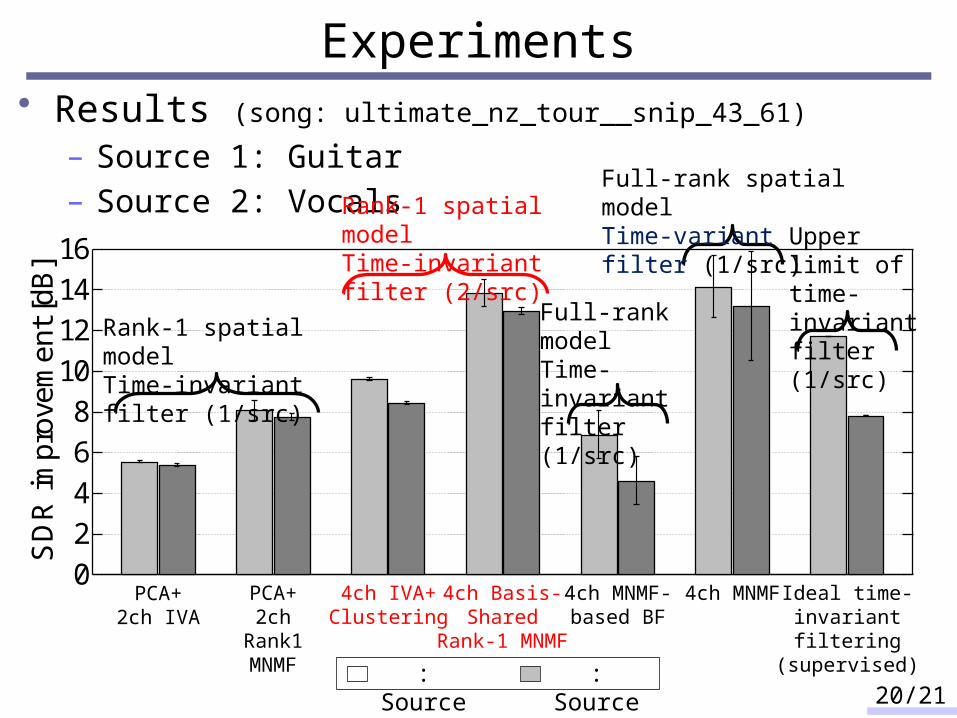
• Results (song: ultimate_nz_tour__snip_43_61)

– Source 1: Guitar– Source 2: Vocals1614121086420

SD

R im

prov

emen

t [dB

]Experiments

20/21

Rank-1 spatial modelTime-invariant filter (1/src)

Full-rank modelTime-invariant filter (1/src)

Full-rank spatial modelTime-variant filter (1/src)

Upper limit of time-invariant filter (1/src)

Rank-1 spatial modelTime-invariant filter (2/src)

: Source 1 : Source 2

PCA+2ch IVA

PCA+2ch Rank1

MNMF

4ch IVA+Clustering

4ch MNMF-based BF

4ch MNMF Ideal time-invariant filtering

(supervised)

4ch Basis-Shared Rank-1

MNMF

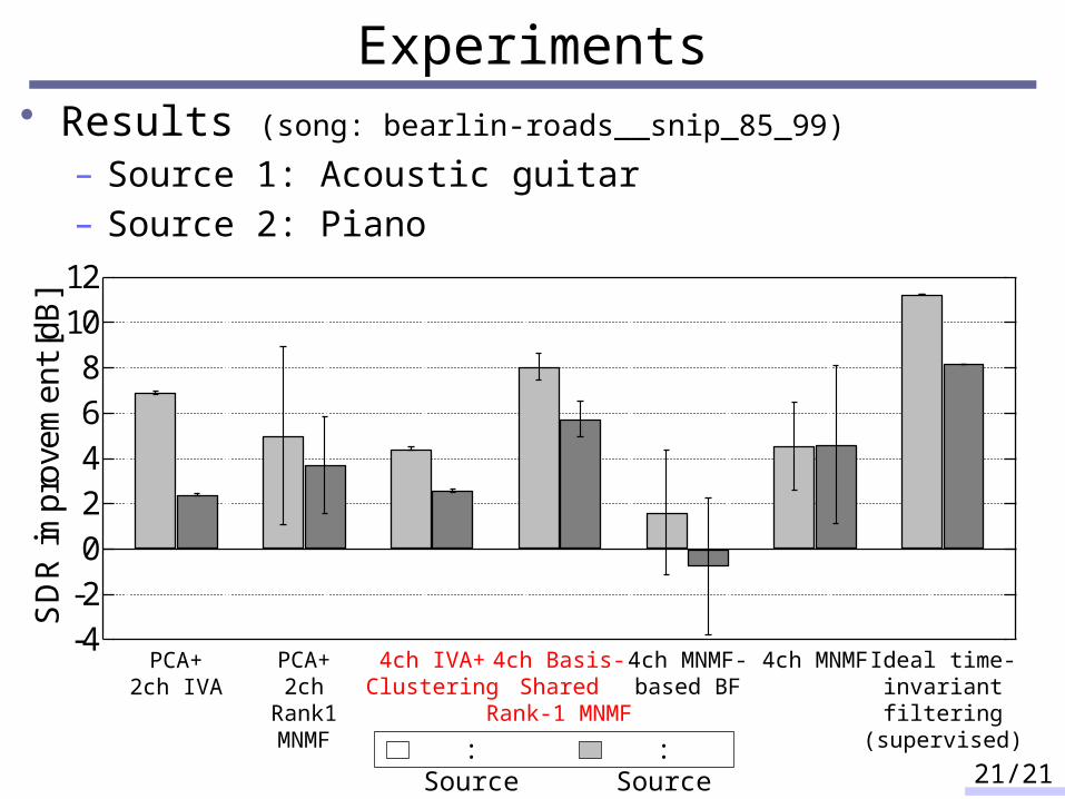
• Results (song: bearlin-roads__snip_85_99)

– Source 1: Acoustic guitar– Source 2: Piano121086420-2-4

SD

R im

prov

emen

t [dB

]Experiments

21/21: Source 1 : Source 2

PCA+2ch IVA

PCA+2ch Rank1

MNMF

4ch IVA+Clustering

4ch MNMF4ch Basis-Shared Rank-1

MNMF

Ideal time-invariant filtering

(supervised)

4ch MNMF-based BF

Experiments

22/21

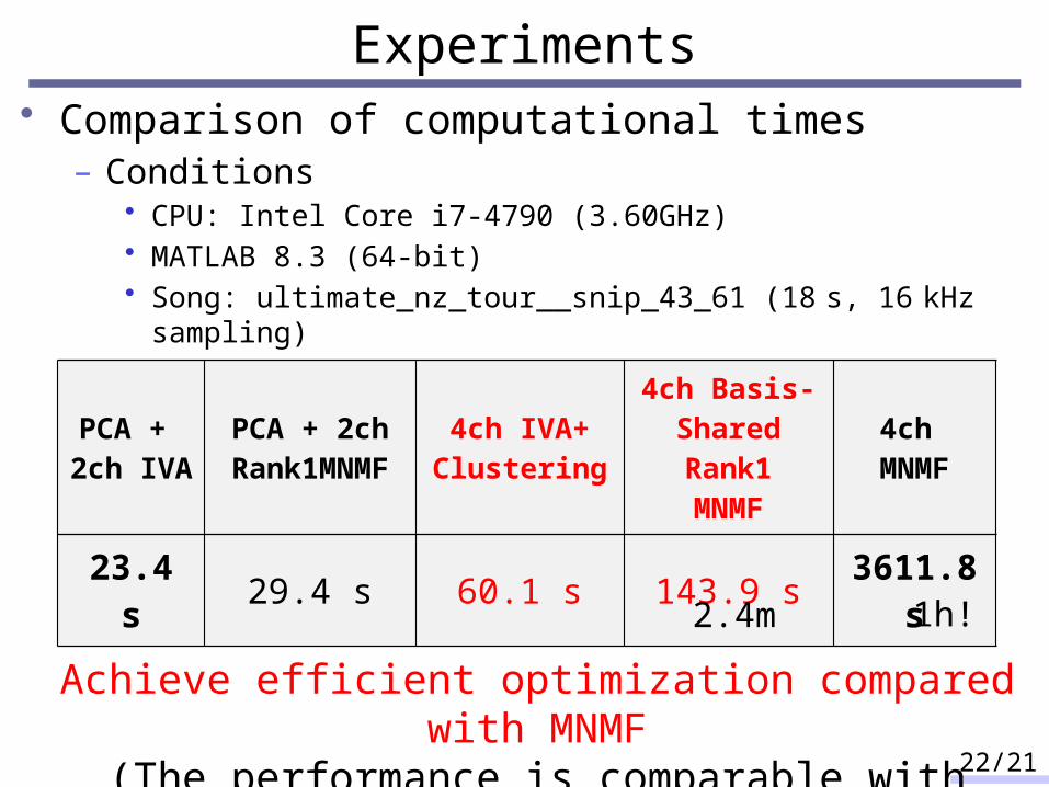
• Comparison of computational times– Conditions

• CPU: Intel Core i7-4790 (3.60GHz)• MATLAB 8.3 (64-bit)• Song: ultimate_nz_tour__snip_43_61 (18 s, 16 kHz sampling)

PCA + 2ch IVA

PCA + 2ch Rank1MNMF

4ch IVA+Clustering

4ch Basis-Shared Rank1

MNMF4ch

MNMF

23.4 s 29.4 s 60.1 s 143.9 s 3611.8 s

Achieve efficient optimization compared with MNMF(The performance is comparable with MNMF)

1h!2.4m

Conclusion• For the case of reverberant signals

– Achieve both good performance and efficient optimization• The proposed method

– Can be applied when the number of microphones is grater than twice the number of sources

– separately estimates direct and reverberant components utilizing extra observations

– can be thought as a relaxation of rank-1 spatial constraint• Experimental results show better performance

– The proposed method outperforms the upper limit of time-invariant filtering in some cases

23/21Thank you for your attention!

relaxation of rank-1 spatial constraint in overdetermined blind source separation

Technology