Relativity and Structure in Neutron Stars

Brian Friesen

December 9, 2011

Abstract

We explore the structure of neutron stars using the Tolman-Oppenheimer-Volkoffequation of hydrostatic equilibrium, the solution to which describes the complete me-chanical structure of a spherically symmetric, self-gravitating, static mass in generalrelativity. We close this equation by supplying a nuclear equation of state and cal-culate mass-radius and mass-central density relations, giving particular attention tothe maximum mass predicted for a neutron star with this equation of state. Finallywe compare these predictions to those from other work in the literature and discussconstraints imposed by neutron star masses inferred from observations.

1 IntroductionNeutron stars (NSs) are compact celestial objects which display some of the most exoticphysical behavior of any objects in the observable universe. With mass densities of ∼ 5×1015

g cm−3 and Fermi energies of ∼ 100 MeV, NS matter is more dense than nuclear matter,ρnuc ∼ 1014 g cm−3, and even at the high temperatures characteristic of NSs (106 − 108 K),this enormous density renders much of it degenerate. At the macroscopic scale the matterproduces gravitational fields so strong that general relativistic effects become substantial,rendering the Newtonian theory of gravity insufficient for predicting the physical propertiesof these stars.

This paper focuses primarily on the effects of general relativity on the structure of neutronstars, while also giving some attention to aspects of nuclear physics relevant in constructingthe nuclear equation of state (EOS). Specifically we explore the structure of a simple neutronstar model: a spherically symmetric, uncharged, non-rotating mass composed of a perfect(incompressible) fluid in general relativistic spacetime. This work is based on foundationalcalculations performed by Tolman 1939 and Oppenheimer and Volkoff 1939, but improvesupon them by using more realistic EOSs as well as sophisticated numerical methods.

In Section 2 we review briefly the current NS observational efforts and results; next, inSection 3 we introduce the Tolman-Oppenheimer-Volkoff (TOV) differential equations andthe properties of the spacetime from which they are constructed; in Section 4 we reviewproperties of the EOS used to close this system of equations (this discussion is only cursory,given the complexity of nuclear theory); in Section 5 we discuss the role the TOV equations

1

play in analyzing neutron star observations; Section 6 contains an overview of the numericalmethods we have applied in solving these equations. Finally, in Section 7 we analyze ourresults and compare them both to other calculations existing in the literature, as well as toobservations.

2 Neutron Star ObservationsAn NS forms when the core of a massive star (& 8M�) exhausts its nuclear fuel, with onlyiron “ash” remaining, and collapses under extreme gravitational pressure. During collapsethe iron nuclei deleptonize via electron capture and eventually the density becomes so largethat the short-range repulsive component of the strong force overwhelms that of gravity,causing the core to rebound and ejecting the outer layers of the star. This is a core-collapsesupernova. What remains is a rapidly rotating mass of neutron-rich material with a strongmagnetic field: a NS.

The angular velocity of NSs varies but can be as high as several 100 Hz; however rotationdecelerates over time due to angular momentum loss from energy radiated away in theirmagnetic fields. Rapidly rotating NSs with misaligned magnetic and rotational axes emitintense beams of radio waves from their magnetic poles and appear to “pulse” as one polesweeps across the Earth. These pulsars and were first discovered in 1967 (Hewish et al. 1968).However older NSs which have slowed significantly cease pulsating entirely (even though theyare still rotating) and are much more difficult to detect (Chen and Ruderman 1993). So faronly a handful have been discovered, the first in 1996 (Walter, Wolk, and Neuhäuser 1996).The difficulty in detecting these “plain” neutron stars stems from a combination of theirblackbody-like nature and their small size. Such difficulty is evident through the followingcalculation. According to the Stefan-Boltzmann law the luminosity L of a blackbody withradius R and temperature T is

L = 4πR2σT 4 (1)

where σ ' 5.67× 10−5 erg cm−2 s−1 K−4 is the Stefan-Boltzmann constant. Shortly after aneutron star is born it has a temperature of ∼ 1011 K but cools quickly via neutrino emissionand spends most of its life at ∼ 106 K (Heiselberg and Pandharipande 2000). Combiningthis temperature with the compactness of these objects (a typical radius is 10 km), we canestimate their total luminosity:

LNS ∼ 4π(10 km)2σ(106 K)4 ∼ 1033 erg s−1 ∼ 1L�. (2)

Even though a neutron star can be as bright as the Sun, due to its high temperature itsspectral energy distribution peaks at a much shorter wavelength than does that of the Sun.One may calculate this peak using Wien’s displacement law:

λmaxT ' 2.90× 10−3 m ·K (3)

which for a 106 K blackbody corresponds to λmax ' 3 nm, in the X-ray portion of the electro-magnetic spectrum. The Earth’s atmosphere is opaque to radiation at this energy, limiting

2

neutron star detectors to space-based observatories. Since the first X-ray observatories werebuilt only in the 1970s (X-ray Astronomy 2010) it is not surprising that the first detectionof an isolated NS occured just 15 years ago.

In Fig. 1 is contained a current list of neutron star masses inferred from observations,organized by the type of binary star system in which the star was found.1 The spread inmass shown in this figure is considerable, ranging from 0.7M� to nearly 3M�. The averagemasses of each group are shown as vertical dotted lines, and error-weighted average massesare shown as vertical dashed lines. In each type of NS binary system both averages are closeto 1.4M�. The most striking of these is J1748-2021B, a ∼ 2.8M� NS, by a wide margin themost massive NS ever detected (Freire et al. 2008). In the following sections we will showhow in the largest of these observed masses, with this object in particular, play a centralrole in constraining the nuclear EOS.

3 The Tolman-Oppenheimer-Volkoff (TOV) equationHaving reviewed the observational progress and difficulties of NSs we now turn to the math-ematical construction of neutron star models. In 1939 R. C. Tolman, J. R. Oppenheimer andG. M. Volkoff solved the Einstein field equations for a perfect, self-gravitating, non-rotating,spherically symmetric, hydrostatic fluid (Oppenheimer and Volkoff 1939; Tolman 1939). Theresult, based on the interior Schwarzschild metric of the form

ds2 = −eΦ(r)(cdt)2 +

(1− 2Gm(r)

c2r

)−1

dr2 + r2(dθ2 + sin2 θdφ2) (4)

is an integro-differential equation for the pressure p which bears their names,

dp

dr= −Gm(r)ρ(r)

r2

(1 +

p(r)

ρ(r)c2

)(1 +

4πr3p(r)

m(r)c2

)(1− 2Gm(r)

c2r

)−1

(5)

(see Appendix for a derivation) where

m(r) ≡∫ r

0

4πρ(r′)r′2dr′, (6)

and ρ is the mass-energy density:

ρ(T ) ≡ ρ0

(1 +

ε(T )

c2

)(7)

1Most of these NSs are in fact rotating pulsars. There exist analytic solutions to the Einstein equations forrotating spherical masses (see Kerr 1963) but calculations in this spacetime are enormously more complicatedthan those in non-rotating Schwarzschild spacetime and are beyond the scope of this discussion (see Hartle1967). Fortunately for us, however, the effects of rotation on internal NS structure are insignificant exceptin objects with periods . 1 ms. (Heiselberg and Pandharipande 2000).

3

where ρ0 is the rest mass, ε is the internal energy per baryon and T is the baryon temperature(Baumgarte and Shapiro 2010). The TOV solution also provides a differential equation forthe metric component Φ(r):

dΦ

dr=

2Gm(r)

c2r2

(1 +

4πr3p(r)

m(r)c2

)(1− 2Gm(r)

c2r

)−1

. (8)

There are some illuminating features of the TOV equation which deserve some attention.First, this equation is nothing more than the Newtonian differential equation of hydrostaticequilibrium with a few multiplicative correction terms. In the non-relativistic limit (c → ∞)each of these corrections goes to unity. Second, each of the three correction terms is > 1, sorelativistic effects always lead to a steeper pressure gradient in the star than in the Newtoniancase. Third, in both the relativistic and non-relativistic cases, the RHS of the dp/dr equationis negative throughout the star; this means that p(r) in every model decreases monotoni-cally as r increases. (This last feature in particular is helpful in establishing boundaries onphysically reasonable models, as we will discuss below.) Finally, the integrand in Eq. 6 isnot simply ρdV for a spherically symmetric shell in this spacetime. To show this we recallthat in general the 4-volume element dV is

dV =√−gd4x (9)

where g ≡ det gαβ , and gαβ is the metric tensor. For constant t (this is a hydrostatic model)the 3-volume element for a spherical shell in these coordinates is then

dV = 4πr2(√grrdr) = 4πr2

(1− 2Gm(r)

c2r

)−1/2

dr (10)

For dV to remain finite, r > 2Gm(r)/c2, in which case dV (r) ≥ 4πr2dr. Therefore Eq. 6will always be smaller than

∫ρdV . The negative contribution comes from the gravitational

binding energy of the star.One can transform the TOV integro-differential equation into two first-order differential

equations by applying the Leibniz integral rule:

d

dx

[∫ g(x)

f(x)

h(x, y)dy

]=

(dg

dx

)h(g, x)−

(df

dx

)h(f, x) +

∫ g(x)

f(x)

∂

∂x[h(x, y)]dy. (11)

Applying this to m(r), we havedm

dr= 4πρ(r)r2. (12)

We writem(r) as an ODE rather than as an integral for simplicity in its numerical integration.We then have three ordinary differential equations (5, 8 and 12) for four variables (p,

ρ, m and Φ). To solve the system uniquely we require a fourth equation as well as threeboundary conditions, one for each of the three first-order ODEs. However we note herethat, in the course of solving the TOV system, we will neglect the solution for Φ(r). The

4

reasons are twofold: first, because neither p(r) nor m(r) depend on Φ(r), one need notintegrate it simultaneously with p(r) and ρ(r). Second, the physical interpretation of Φ(r)is of limited utility for our purposes in this paper; it describes the dilation or contractionof the coordinate time t and therefore contains information about the gravitational redshiftof radiation emitted from the star, but the star’s mechanical structure, with which we arechiefly concerned in this work, is unaffected by this quantity. In this case, we have only twoODEs (5 and 12) for three variables, p, ρ and m. We still require an equation relation p toρ, as well as two boundary conditions for the two ODEs.

The EOS provides the link between p and ρ. To construct an EOS of the form P = P (ρ, T )we turn to the first law of thermodynamics:

dU ≡ TdS − pdV +∑i

µidNi (13)

where U is the total internal energy, S is the entropy, V is the fluid volume, µi and Ni arerespectively the chemical potential and the number population of species i. A perfect fluidis isentropic so dS = 0, and its particle number is conserved so dN = 0. Then we have

dU = −pdV. (14)

If we define U and V as the energy and volume per baryon, respectively, then we may write

V ≡ 1

nb→ dV = − 1

n2b

dnb (15)

where nb is the baryon number density. From the definition of ρ,

dU = d(ρc2), (16)

in which casep = n2

b

d(ρc2)

dnb(17)

Since ρ = ρ(ρ0, T ), we now have p = p(ρ0, T ) as desired. Most EOSs use Eq. 17, not Eq. 7to calculate p.

There exists in the TOV equation no constraint on T ; therefore to use a proper two-parameter EOS one must provide by some other means the complete temperature structureof the star. Fortunately even a poor guess for T (r) should play a minor role in the overallstructure of the star: in much of the NS the matter is at least as dense as nuclear matter(nnuc ∼ 0.16 fm−3), leading to Fermi energies of several 10 MeV (Heiselberg and Pandhari-pande 2000). The thermal contribution even at 106 K is only kT ∼ 100 eV and is thereforenegligible.

Despite the meager influence of thermal energy on the NS structure, a mere guess at T isundesirable. One solution is to exploit the isentropic nature of perfect fluids, in which casewe may set T , p and ρ implicitly by forcing the EOS to follow an adiabat, along which theentropy S is constant. Alternatively, and more simply, we may assume the NS is isothermaland fix T everywhere. The latter is an especially popular choice; in fact, many workerssimply set T = 0.

5

4 The Nuclear Equation of StateThe nuclear EOS connects thermodynamic variables such as pressure, energy density andtemperature, in a system composed of nuclear matter. It is of particular astrophysical interestbecause of its pivotal role in driving the dynamics of core-collapse supernova explosions, theresult of which is the formation of neutron stars. However its precise nature continues toelude both the particle physics and astrophysics communities due to large uncertainties inthe theory of the strong interaction, which is responsible for interactions among nucleons(Danielewicz 2001). A thorough study of the nuclear EOS requires a formidable commandof quantum chromodynamics and a detailed discussion is beyond the scope of this work.Instead we examine in some detail a phenomenologically constructed EOS which containsboth experimental and theoretical underpinnings, from Bethe and Johnson 1974 (BJ74).

4.1 The Liquid Drop Model

Many nuclear EOSs are based on an empirical model of the nucleus called the liquid dropmodel. (Incidentally the EOS we have chosen for calculations in this work is not, but theliquid drop model is popular enough that it nonetheless warrants a review here.) First sug-gested by G. Gamow, this model attempts to calculate the nuclear mass and binding energyusing a number properties found in macroscopic liquid drops; in particular it assumes thatthe interior density is constant, and that the total binding energy of a nucleus is propor-tional to its mass (Martin 2009). C. F. von Weizsäcker quantified these and other propertiesthrough an equation called the semi-empirical mass formula (SEMF), which describes thetotal mass of the nucleus:

M(Z,A) = Z(Mp +me) +Mn(A− Z)− a1A+ a2A2/3 (18)

+ a3Z(Z − 1)

A1/3+ a4

(Z − A

2

)2

A+ f5(Z,A). (19)

The first two terms represent the fermionic content of the nucleus: Z is the atomic number,A is the atomic weight,Mp is the proton mass,Mn is the neutron mass andme is the electronmass.

The next five terms contain correction factors, with ai > 0. The third term on the RHS,−a1A, is a volume correction term, which accounts for the saturation of the strong force,causing only neighboring nucleons to interact with one another via gluon exchange. (TheCoulomb and gravitational forces, in contrast, exhibit no such saturation.) Experimentalevidence shows that the nuclear radius goes like A1/3, so the volume, or mass, goes like(A1/3)3 = A. It is the only of the five correction terms in the SEMF which contributesto the binding energy and reduces the nuclear mass. The fourth term, a2A

2/3, accountsfor an overestimation in the volume correction term, since nucleons on the surface of thenucleus are not surrounded. The term is proportional to the surface area, which goes likethe square of the radius, or (A1/3)2 = A2/3. The next term, a3

Z(Z−1)

A1/3 , represents the Coulombinteractions among the protons in the nucleus. The penultimate term, a4

(Z−A/2)2

A, accounts

6

for the tendency of nuclei to have equal numbers of protons and neutrons. The last term isa pairing term,

f5(Z,A) =

−a5A

−1/2 if Z,N even+a5A

−1/2 if Z,N odd0 otherwise

(20)

which describes the tendency of like nucleons in the same spatial state to couple, producingan overall spin-0 state (Martin 2009).

4.2 Bethe and Johnson (BJ74)

Rather than fitting mass and simple binding energy formulae to experimental data as mostSEMF-based EOSs do, BJ74 instead calculates nucleon-nucleon interactions directly usingnon-relativistic, many-body theory. The strong force is modeled empirically by accounting forits attraction between distant nucleons and repulsion between nearby nucleons. Physicallythey assume the long-distance attractive component is due to exchange of scalar mesons(that is, spin-0 mesons with even parity), while the short-range repulsive core is due toexchange of vector mesons (spin-1 mesons with odd parity); mathematically they representthis interaction using a Reid core potential (Reid 1968), which consists of attractive andrepulsive Yukawa potentials:

VAB = (µr)−1∑n

Cn(AB)e−nµr (21)

where the Cn are positive or negative coefficients whose values depend on the interactingnucleons A and B as well as the angular momenta of each, and µ ≡ mc/~ is the reciprocalCompton wavelength of the meson (with mass m) exchanged between the two nucleons. Itis these coefficients, rather than those discussed in the previous subsection, which are fittedto experimental results, specifically phase shifts in nucleon scattering. BJ74 modify slightlythe Reid core, in that while Reid required n ∈ Z, BJ74 allow n ∈ R. There are many moredetails in this EOS than are presented here, and we refer the interested reader to Bethe andJohnson 1974.

5 TOV’s Role in Compact Object AstrophysicsOne noteworthy feature of self-gravitating compact objects such as NSs is the existence of afinite maximum mass. That is, for a given nuclear EOS there exists a single central densityρc which produces the most massive star possible in stable mechanical equilibrium. Starswith lower masses than this are also stable, but those above are not and therefore do notexist in nature. In neutron stars this mass is called the TOV mass or the TOV limit, whichin 1939 Tolman, Oppenheimer and Volkoff calculated to be about 0.7M�. As will be shownbelow, this value is much lower than predictions with current models. The reason is that theauthors assumed the NS is composed of a completely degenerate, non-interacting neutron

7

gas, the EOS for which is extremely “soft,” meaning a small change in P causes a largechange in ρ.

Astronomers and particle physicists alike place such faith in the predictions of generalrelativity that one of their primary methods of constraining the nuclear EOS (which remainslargely unknown) consists of observing neutron star masses and comparing them with thelargest masses predicted by various EOSs (Lattimer and Prakash 2005; Lattimer 2007). Thattwo branches of physics conspire across so many orders of magnitude in scale to answer asingle scientific query illustrates a truly remarkable property of the TOV model.

6 Numerical MethodsThe TOV differential equations for p and m are coupled and therefore must be integratedsimultaneously; the equation for Φ, however, is decoupled and can be solved after p(r) andm(r) have been found, although we will not do so in this work. The P and ρ ODEs are wellbehaved (non-singular, non-oscillatory, etc.) in the domain r > 0 and p > 0 and thereforemay be integrated using even very simple numerical methods.

We have written a code2 in C called TOV_solver which integrates the TOV equationsusing the fifth-order Runge-Kutta Dormand-Prince algorithm (Dormand and Prince 1980).The code calls the EOS in a modular way such that the user may use any EOS he wishes.Alternatively, if an EOS cannot easily be incorporated into the code, or if its source code isnot publically available, TOV_solver can interpolate thermodynamic data from tables. Mostpublic EOSs such as Ishizuka et al. 2008, Cooperstein 1985 and Timmes and Swesty 2000 arewritten in “callable” form, in anticipation of being used in a wide variety of simulation codes.TOV_solver exploits this fact and consequently may be used to constrain the nuclear EOSby comparing their maximum predicted masses of neutron stars with those masses inferredfrom observation.

Before we can integrate the TOV equations we must specify boundary conditions. First,as discussed at length in Oppenheimer and Volkoff 1939 the only value of m(r = 0) ≡ mc

which prevents the metric tensor component grr from diverging is mc = 0. Also, we definethe surface of the star as the location R where p(r = R) = 0. The only free parameter inthis system of equations is therefore ρ(r = 0) ≡ ρc. Setting this value manually allows usto integrate the TOV equation and calculate the complete mechanical structure of the star,including its total mass m(r = R) ≡M .

7 Analysis of Results

7.1 Thermodynamic Predictions of BJ74

Before showing any NS calculations we first show some of the characteristic thermodynamicproperties of BJ74 in Fig. 2. In this plot and throughout this work we have used T = 0,

2The source is freely available at GitHub: http://git.io/QUGTIg.

8

owing to the insignificance of thermal effects. In the majority of this plot the EOS followsa nearly straight line in the log-log plot, corresponding to a power-law relationship, thevalue of the power being equal to the slope of the line. It is for this reason that polytropic(power-law) representations of EOSs, which have the form p ∼ ρΓ, remain so popular.

7.2 Internal NS Structure

We now explore the structure of a typical NS through the relations p(r), m(r) and ρ(r)for a given EOS and ρ0. However we must first address a complication which plagues allcalculations performed in GR, namely that the curvature of spacetime changes the physicalrepresentation of the coordinates chosen for the calculation. In this case the problem liesin that the proper length ds as defined in Eq. 4 is not linear in the coordinate dr. In flatspacetime we could write the metric as

ds2 = −(cdt)2 + dr2 + r2(dθ2 + sin2 θdφ2) (22)

in which case one could treat r exactly as in a solid, Euclidean 2-sphere: at a given fixedtime t it is a coordinate whose value is zero at the center of the sphere, reaches a maximumat the sphere’s surface, and increases linearly along a geodesic connecting those two points.

In the interior Schwarzschild spacetime, however, this is no longer the case, and wemust scrutinize the “radial curvature” in order to determine if we can perform at least aqualitatively accurate analysis of the NS using r as a radius. (In the exterior Schwarzschildsolution the radial coordinate r diverges as one approaches the Schwarzschild radius, eventhough the spacetime at that point is physically well-behaved.) One way to do this is tocalculate the Riemann tensor Rαβγδ, the Ricci tensor Rαβ or the curvature scalar R as afunction of r. However we choose a slightly more intuitive approach: we calculate thestructure of a NS with ρ0 = 1015 g cm−3 using BJ74, and in Fig. 3 we plot the quantityds/dr, which is just (1− 2Gm(r)/c2r)−1/2, versus r. A value of unity in this figure indicatesflat spacetime. If the space were flat or nearly so, we could perform this calculation usingthe much simpler Newtonian formulation of gravity. We see in the figure that deviationsfrom unity are significant, with |(dL/dr)− 1| . 25%. If we ignored relativistic effects thesedeviations would most likely result in errors of this magnitude or more in the prediction ofthe TOV limit. However the interior coordinate r diverges nowhere within the star, and soin the following qualitative discussions we will treat it as a radius in a Euclidean 2-sphere.

We are now equipped to study the mechanical structure of a typical NS. Again using theBJ74 EOS with ρ0 = 1015 g cm−3, we show m(r) and ρ(r) in Figs. 4 and 5, respectively.Both figures show that the BJ74 result corroborates the canonical NS model which consistsof a super-dense body with a very thin “atmosphere.” The low-density region (in Fig. 4 theregion where m(r) is flat) is very narrow and in Fig. 5 ρ stays nearly constant from the coreall the way to the surface, then drops to zero in a span of ∆r . 1 km.

We note also that the region of maximum spacetime curvature is at r ∼ 10 km in Fig. 3.This corresponds to the location of the majority of the stellar mass as shown in Fig. 4. Thisverifies the intuitive interpretation of the theory of general relativity: more mass (energy)leads to more curvature.

9

7.3 The TOV Limit

Among the most popular calculations performed with the TOV equations with a particularEOS are the mass-radius and mass-central density relations. Pictoral summaries of currentprogress in this field are shown in Fig. 6 (mass-radius) and in Fig. 7 (mass-central density).These figures show a wide distribution of maximum mass predictions, ranging from 1.3 M�to 2.8 M�. One is able to validate (or invalidate) an EOS by calculating the TOV limit andsearching for any observed non-rotating NS masses which are larger. If such stars exist, thenthe EOS must be incorrect or incomplete.

The number of observed NS stars with inferred masses is small, and until a much largersample is compiled, and the observational uncertainties reduced, one cannot use them con-fidently to rule out any EOS. However the results compiled so far are nevertheless quiteinformative. We draw special attention to the pulsar J1748-2021B in Fig. 1, whose mass of2.8M� (with small error bars) is so far the largest of any observed NS. It is also larger thanthe TOV limit of nearly every EOS in Figs. 6 and 7. The discovery of this pulsar, if itsinferred mass is correct, will have profound effects on the study of the nuclear EOS, sincenearly every one is too soft to attain a mass so large.

In Fig. 8 we show the mass-central density relation for BJ74, and in Fig. 9 we showthe mass-radius relation. BJ74 predicts a maximum NS mass of ∼ 1.9M�, which is slightlylower than the average of the EOSs show in Fig. 6, but toward the upper end of the observedmasses in Fig. 1. Not only is its maximum mass prediction close to those of other EOSs, butalso does the overall shape of its mass-radius and mass-central density relations. However,like the other EOSs, its TOV limit falls well below the 2.8M� of the pulsar J1748-2021B.

8 SummaryWe have developed the mathematical framework to calculate the complete mechanical struc-ture of a spherically symmetric, non-rotating, static mass composed of a perfect fluid ingeneral relativity. Within this framework we have included a modern nuclear EOS, BJ74,in order to calculate the maximum mass of a non-rotating neutron star. This EOS predicts∼ 1.9M�, in rough agreement with other EOSs. We have also compared this result to alist of observed NS masses and found it be larger than most. However BJ74 and almostevery other nuclear EOS appear to conflict with a recently discovered 2.8M� pulsar which, ifthe mass estimate of this object is accurate, indicates that there exists some crucial nuclearprocesses which have yet to be discovered.

ReferencesBaumgarte, Thomas W. and Stuart L. Shapiro (2010). Numerical Relativity: Solving Ein-

stein’s Equations on the Computer. Cambridge, UK: Cambridge University Press.

10

Bethe, H.A. and M.B. Johnson (1974). “Dense baryon matter calculations with realisticpotentials.” In: Nuclear Physics A 230.1, pp. 1 –58. issn: 0375-9474. doi: 10.1016/0375-9474(74)90528-4. url: http://www.sciencedirect.com/science/article/pii/0375947474905284.

Chen, K. and M. Ruderman (Jan. 1993). “Pulsar death lines and death valley.” In: Astro-physical Journal 402, pp. 264–270. doi: 10.1086/172129.

Cooperstein, J. (1985). In: Nucl. Phys. A438, p. 722.Danielewicz, Paweł (2001). “Nuclear equation of state.” In: AIP Conference Proceedings

597.1. Ed. by Xizhen Wu et al., pp. 24–42. doi: 10.1063/1.1427443. url: http://link.aip.org/link/?APC/597/24/1.

Dormand, J.R. and P.J. Prince (1980). “A family of embedded Runge-Kutta formulae.” In:Journal of Computational and Applied Mathematics 6.1, pp. 19 –26. issn: 0377-0427.doi: 10.1016/0771-050X(80)90013-3. url: http://www.sciencedirect.com/science/article/pii/0771050X80900133.

Freire, P. C. C. et al. (Mar. 2008). “Eight New Millisecond Pulsars in NGC 6440 and NGC6441.” In: Astrophysical Journal 675, pp. 670–682. doi: 10.1086/526338. arXiv:0711.0925.

Hartle, J. B. (Dec. 1967). “Slowly Rotating Relativistic Stars. I. Equations of Structure.” In:Astrophysical Journal 150, p. 1005. doi: 10.1086/149400.

Heiselberg, Henning and Vijay Pandharipande (2000). “RECENT PROGRESS IN NEU-TRON STAR THEORY.” In: Annual Review of Nuclear and Particle Science 50.1,pp. 481–524. doi: 10.1146/annurev.nucl.50.1.481. eprint: http://www.annualreviews.org/doi/pdf/10.1146/annurev.nucl.50.1.481. url: http://www.annualreviews.org/doi/abs/10.1146/annurev.nucl.50.1.481.

Hewish, A. et al. (Feb. 1968). “Observation of a Rapidly Pulsating Radio Source.” In: Nature217, pp. 709–713. doi: 10.1038/217709a0.

Hughston, L. P. and K. P. Tod (1990). An Introduction to General Relativity. Cambridge,UK: Cambridge University Press.

Ishizuka, C. et al. (Aug. 2008). “Tables of hyperonic matter equation of state for core-collapse supernovae.” In: Journal of Physics G Nuclear Physics 35.8, p. 085201. doi:10.1088/0954-3899/35/8/085201. arXiv:0802.2318 [nucl-th].

Kerr, Roy P. (1963). “Gravitational Field of a Spinning Mass as an Example of AlgebraicallySpecial Metrics.” In: Phys. Rev. Lett. 11 (5), pp. 237–238. doi: 10.1103/PhysRevLett.11.237. url: http://link.aps.org/doi/10.1103/PhysRevLett.11.237.

Lattimer, J. M. and M. Prakash (2001). “Neutron Star Structure and the Equation of State.”In: The Astrophysical Journal 550.1, p. 426. url: http://stacks.iop.org/0004-637X/550/i=1/a=426.

Lattimer, J. M. and M. Prakash (Mar. 2005). “Ultimate Energy Density of Observable ColdBaryonic Matter.” In: Physical Review Letters 94.11, 111101, p. 111101. doi: 10.1103/PhysRevLett.94.111101. eprint: arXiv:astro-ph/0411280.

11

Lattimer, James (2007). “Equation of state constraints from neutron stars.” In: Astrophysicsand Space Science 308 (1). 10.1007/s10509-007-9381-3, pp. 371–379. issn: 0004-640X.url: http://dx.doi.org/10.1007/s10509-007-9381-3.

Martin, B. R. (2009). Nuclear and Particle Physics. 2nd. Chichester, West Sussex, UK: JohnWiley & Sons Ltd.

Oppenheimer, J. R. and G. M. Volkoff (Feb. 1939). “On Massive Neutron Cores.” In: PhysicalReview 55, pp. 374–381. doi: 10.1103/PhysRev.55.374.

Reid, Roderick V. (1968). “Local phenomenological nucleon-nucleon potentials.” In: Annalsof Physics 50.3, pp. 411 –448. issn: 0003-4916. doi: 10.1016/0003-4916(68)90126-7.url: http://www.sciencedirect.com/science/article/pii/0003491668901267.

Timmes, F. X. and F. D. Swesty (Feb. 2000). “The Accuracy, Consistency, and Speed of anElectron-Positron Equation of State Based on Table Interpolation of the Helmholtz FreeEnergy.” In: Astrophysical Journal Supplement 126, pp. 501–516.

Timmes, Frank X. (Nov. 2011). Cold Neutron Stars. url: http://cococubed.asu.edu/images/nstar/rho_mass_web_large.jpg.

Tolman, R. C. (Feb. 1939). “Static Solutions of Einstein’s Field Equations for Spheres ofFluid.” In: Physical Review 55, pp. 364–373. doi: 10.1103/PhysRev.55.364.

Walter, F. M., S. J. Wolk, and R. Neuhäuser (Jan. 1996). “Discovery of a nearby isolatedneutron star.” In: Nature 379, pp. 233–235. doi: 10.1038/379233a0.

X-ray Astronomy (Dec. 2010). url: http://imagine.gsfc.nasa.gov/docs/science/know_l2/history_xray.html.

12

Figure 1: A list of neutron star masses inferred from observations of binary systems. Thevertical dotted lines indicate the average masses in each type of system; the dashed lines areerror-weighted averages. This figure is an updated version of Fig. 2 of Lattimer and Prakash2005.

13

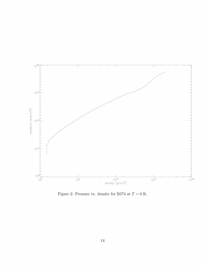
Figure 2: Pressure vs. density for BJ74 at T = 0 K.

14

Figure 3: Comparison of geodesic length ds with “radial” coordinate length dr for a NS usingBJ74 with a central density of ρ0 = 1015 g cm−3 (solid line). A value of ds/dr = 1, shown asthe dotted line, indicates s is linear in r, i.e., the spacetime is flat along the radial direction.The NS spacetime deviates up to 25% from the flat spacetime result, showing that neglectingGR effects could results in errors of this magnitude or larger.

15

Figure 4: Inclusive mass vs. radius for a NS using BJ74 with ρ0 = 1015 g cm−3.

16

Figure 5: Mass density vs. radius for a NS using BJ74 with ρ0 = 1015 g cm−3.

17

Figure 6: Mass-radius relation for neutron stars according to different nuclear EOSs. Thisfigure is Fig. 7 of Lattimer and Prakash 2001. The predicted maximum masses as well astheir corresponding radii are quite disparate.

18

Figure 7: Mass-central density relation for neutron stars with different EOSs. Taken fromTimmes 2011.

19

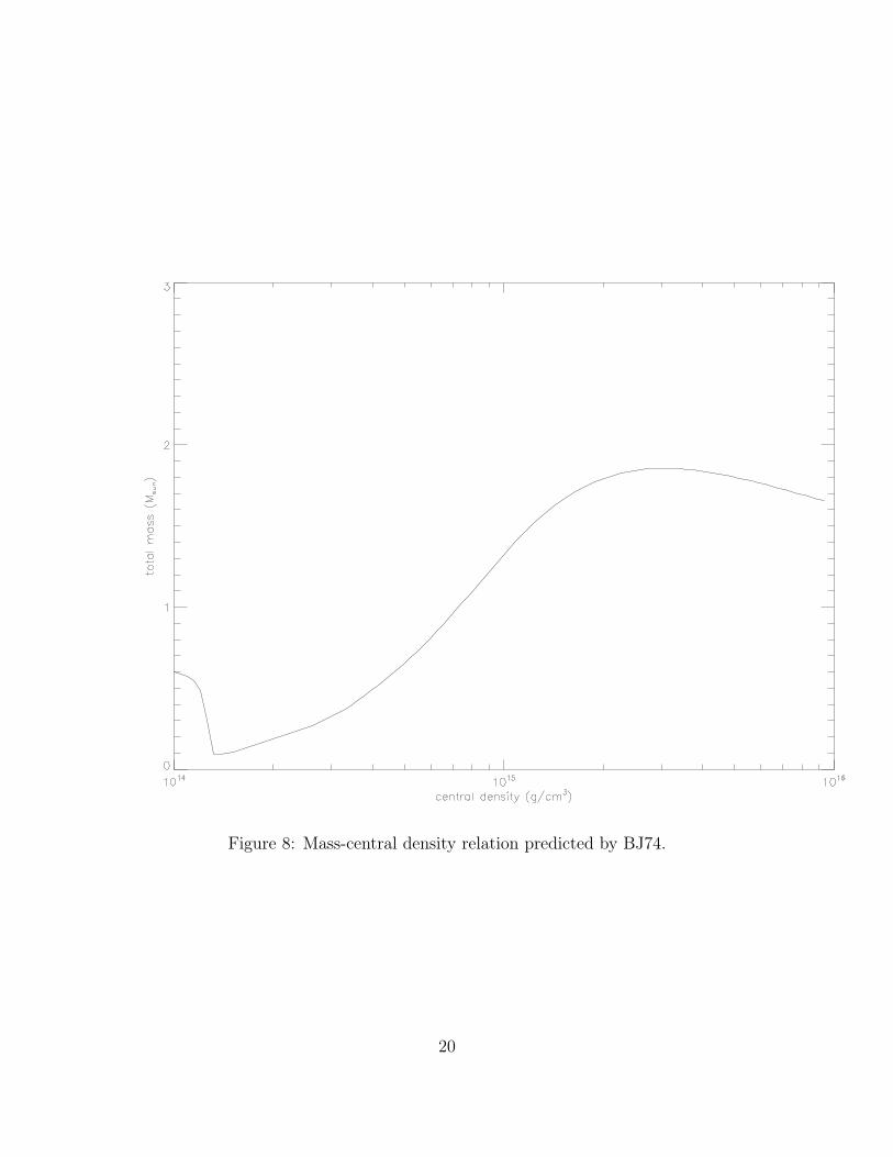
Figure 8: Mass-central density relation predicted by BJ74.

20

Figure 9: Mass-radius relation predicted by BJ74.

21