relativity and covariant electromagnetism · relativity and covariant formulation of the...
TRANSCRIPT

Relativity and Covariant Electromagnetism
Ismael Rodrigues SilvaQueen Mary, University of London
August 2014
Preface
This work is part of my exchange programme in the United Kingdom,written during the summer of 2014, on my year abroad at Queen Mary,University of London. The topics covered are brief introductions to SpecialRelativity and covariant formulation of the Electromagnetism, includingthe consequences from the postulates of Special Relativity, and a step-by-step explanation of Tensor Calculus and Relativistic Mechanics.
Acknowledgements
To my family, which has never stopped believing me, specially mymother Tania. To my advisor at Queen Mary, University of London, Dr.Alston Misquitta, and to my advisor and counselor at Universidade Fed-eral de Santa Catarina, Dr. Marco Kneipp. To my friends, in particularAugusto, Luciano, Madlene, Deborah, Antonio and Maique, who, fromBrazil, have been supporting me in all moments. To my friends whohelped me through my quick journey in the United Kingdom, Fernanda,Cos, Vasily, Vladimir, Ivan, Elena, Marieta, Sophia, Kristina and Mane-tou. To my sponsor, CNPq. To Dr. Brian Wecht from Queen Mary, whonot only tought me Statistical Physics, but also what a lecturer must belike.
1 The Theory of Relativity
1.1 Historical Background
The basis on which Einstein built the special theory of relativity was the factthat Maxwell’s equations predict that the speed of propagation of the electro-magnetic waves is a universal constant, independent of the motion of the sourceor of the detector of the waves. The two postulates of special relativity, formu-lated by Einstein in 1905, are:
1. The laws of physics are the same in all inertial frames of reference;
2. The speed of light in free space has the same value c in all inertial framesof reference.
1

An inertial frame of reference is a frame in which a freely moving bodyproceeds with constant velocity, that is, a frame in which Newton’s first law ofmotion holds or, in other words, in which the velocity of any particle remainsconstant unless there is a net force acting on it. If a system moves with constantvelocity with respect to an inertial reference system, then it is also inertial.
Ordinary mechanics assumes that the propagation of interactions of materialparticles is instantaneous. Experiments show, however, that there is no instan-taneous interaction in nature: there is a finite maximum speed of propagation ofinteraction, which implies that motions of bodies with greater speed are impos-sible, for if such a motion could occur, then by means of it one could realise aninteraction with a speed exceeding the maximum possible speed of propagationof interaction. From the second postulate, it follows that this maximum speedis the same in all inertial systems of reference. This universal constant, whichis also the speed of light in free space, designated by c, exactly given by1
c = 2.99792458 · 108m/s. (1)
The mechanics based on the principle of relativity stated above is said tobe relativistic. If the speeds involved are much less than c, the mechanics iscalled classical or Newtonian. Time is absolute in classical mechanics, andso there is one time for all reference frames, what makes simultaneity is anabsolute concept. This is a contradiction in special relativity though. If we usethe general law of combination of velocities to the propagation of interaction,then the speed of propagation would be different in different inertial frames ofreference. Once time is not absolute, simultaneous events in one frame may notbe simultaneous in other frames.
The principle of relativity introduces then drastic and fundamental changesin basic physical concepts. The notion of space and time which we have areonly approximations due to the fact that the speeds with which we deal dailyare very small compared to the speed of light.
1.2 Intervals
An event is described by the place where it occurred and time when it occurred.It is useful to use a four-dimensional space, whose spatial axes are x, y, z andtemporal axis is ct. In this space, events are points (ct1, x1, y1, z1) called worldpoints, and there corresponds to each particle a line, called world line.2
Consider two inertial reference systems K and K ′, with axes (ct, x, y, z) and(ct’, x’, y’, z’) respectively, moving relative to each other with constant velocity.Suppose that the frames coincide at t = t′ = 0, and consider a flash of lightemanating from their common origin at the instant they coincide. Therefore,
1Originally, one metre was intended to be one ten-millionth of the distance from the Earth’sequator to the North Pole, but since 1983 it has been defined as the length of the path travelledby light in vacuum during a time interval of 1/299,792,458 of a second.
2It is easy to show that to a particle in uniform rectilinear motion there corresponds astraight world line.
2

remembering that the distance travelled by the wave is given by the product ofits speed and the interval of time, the spherical wave front described in K by
x2 + y2 + z2 = (ct)2 (2)
will be described in K ′ by
x′2 + y′2 + z′2 = (ct′)2. (3)
In other words,
c2t2 − x2 − y2 − z2 = 0⇔ c2t′2 − x′2 − y′2 − z′2 = 0. (4)
Homogeneity of space and time and isotropy of space require that the relation-ship between (ct, x, y, z) and (ct′, x′, y′, z′) is linear. In fact, a general linearrelation can be used to find the equations for the transformations of the coor-dinates, but this will be done later in a different simpler way.
Relation (4) motivates us to define the interval s12 between two events asthe scalar
s212 = c2(t2 − t1)2 − (x2 − x1)2 − (y2 − y1)2 − (z2 − z1)2, (5)
where (ct1, x1, y1, z1) are the coordinates of the first event and (ct2, x2, y2, z2)are the coordinates of the second event. The interval can be regarded as thedistance between two world points in our four-dimensional space. If the eventsare infinitely close to each other, the infinitesimal interval ds between them isgiven by3
ds2 = c2dt2 − dx2 − dy2 − dz2. (6)
Expression (5) allows us to have either s212 = 0 or s212 > 0 or s212 < 0. If
c2(t2 − t1)2 > (x2 − x1)2 + (y2 − y1)2 + (z2 − z1)2, (7)
then s212 > 0, and the real number s12 is said to be timelike, and there exists acoordinate system in which the two events occur at the same point in space. If
c2(t2 − t1)2 < (x2 − x1)2 + (y2 − y1)2 + (z2 − z1)2, (8)
then s212 < 0, so s12 is imaginary and is said to be spacelike, and there exists acoordinate system in which the two events occur simultaneously. Finally, if
c2(t2 − t1)2 = (x2 − x1)2 + (y2 − y1)2 + (z2 − z1)2, (9)
then the interval is equal to zero and is said to be null or lightlike.The equivalence in (4) implies that, if the interval in K is null, then so is
the interval in K ′. In other words, it is invariant in this case. It turns out thatthe interval, which is a scalar, is always invariant, as we shall see later using theconcept of four-vectors. Until we get there, assume the interval is invariant.
3This geometry was introduced by H. Minkowski and is called pseudo-euclidean, and thefour-dimensional space mentioned is called Minkowski space.
3

1.3 Proper time
The proper time of an object is defined as the time read by a clock moving withthis object. The proper time interval between two events will be therefore theinterval of time measured in a reference frame in which the two events occur atthe same point in space. Let us use the Greek letter τ to describe the propertime.
Consider the same reference systems K and K ′ moving relative to eachother with constant velocity v, and suppose there is a clock at rest in K ′. Theinfinitesimal interval in K is given by
ds2 = c2dt2 − dx2 − dy2 − dz2. (10)
On the other hand, the clock is at rest in K ′, so that dx′ = dy′ = dz′ = 0, andthe time measured is the proper time. Therefore, being constant the interval,we also have
ds2 = c2dτ2, (11)
and so
c2dτ2 = c2dt2 − dx2 − dy2 − dz2 (12)
or
dτ = dt
√1− dx2 + dy2 + dz2
c2dt2= dt
√1− v2
c2, (13)
since
dx2 + dy2 + dz2
dt2= v2, (14)
where v = |v| is the relative speed between the reference systems K and K ′.Let us now define the velocity coefficient
β ≡ v
c(15)
and the Lorentz factor or Lorentz term
γ ≡ 1√1− v2
c2
=1√
1− β2, (16)
where β = |β| = v/c. This way, equation (13) can be written as
dτ =1
γdt, (17)
and we have the important relation4
4Mathematically, just compare equation (18) with the equation dτ = dτdtdt for the differ-
ential dτ .
4

dτ
dt=
1
γ. (18)
Supposing v is constant, one can integrate (18) and obtain the time intervalindicated by the moving clock in K:∫ t2
t1
dτ
dtdt = τ(t2)− τ(t1) ≡ τ2 − τ1 =
∫ t2
t1
1
γdt =
1
γ(t2 − t1) (19)
or
∆τ =1
γ∆t ≤ ∆t, (20)
once v is always less than or equal to c, so that 0 < 1/γ ≤ 1. Therefore, weconclude that the proper time interval of a moving object is always less thanthe corresponding interval in the rest system. In other words, moving clocksrun slow.
According to (11), we also have dτ = ds/c, so the time interval read by theclock in K ′ is also given by
τ2 − τ1 =1
c
∫ b
a
ds, (21)
taken along the world line of the clock. But, since the clock at rest alwaysindicates a greater time interval than the moving one, we conclude that∫ b
a
ds (22)
has its maximum value if it is taken along the straight world line joining thepoints a and b.
1.4 The Lorentz Transformation
We wish to derive now the formulae for the transformation of coordinates fromone inertial system to another. Consider the same inertial frames K and K ′
with axes ct, x, y, z and ct′, x′, y′, z′ respectively, and suppose that the axes xand x′ are coincident. Let v be the speed of K ′ relative to K, and suppose thatthe origins of the two systems coincide at times t = t′ = 0. We will define thissituation as a boost in x-direction. According to classical mechanics, for theboost described we would have
x′ = x− vt, y′ = y, z′ = z, t′ = t, (23)
or, in matrix form, t′
x′
y′
z′
=
1 0 0 0−v 1 0 00 0 1 00 0 0 1
txyz
, (24)
5

which is called Galilean transformation and is clearly inconsistent with the prin-ciple of relativity once it does not remain constant the interval.
Since the interval can be regarded as the distance between two world pointsin our four-dimensional space, the transformation we seek must be expressiblemathematically as a rotation in this space. Let us consider a rotation in the txplane, so that c2t2 − x2 must be invariant. In the most general case, we have
ct′ = ct cosh ζ − x sinh ζ, x′ = −ct sinh ζ + x cosh ζ (25)
where ζ is called rapidity5. In matrix notation, this is written asct′
x′
y′
z′
=
cosh ζ − sinh ζ 0 0− sinh ζ cosh ζ 0 0
0 0 1 00 0 0 1
ctxyz
, (26)
likewise for a rotation about the z-axisct′
x′
y′
z′
=
1 0 0 00 cos θ sin θ 00 − sin θ cos θ 00 0 0 1
ctxyz
, (27)
so that ζ can be interpreted as a four-dimensional angle of rotation in the txplane.
We wish now to determine ζ, which depends on v. But that is trivial: justconsider the motion, in K, of the origin of K ′. We have then x′ = 0, so thesecond equation in (25) gives us
ct sinh ζ = x cosh ζ (28)
or
x = (c tanh ζ)t, (29)
so that
v =dx
dt= c tanh ζ (30)
or
tanh ζ =v
c= β. (31)
One can now easily find
sinh ζ =β√
1− β2, cosh ζ =
1√1− β2
, (32)
5One can easily check, using the identity cosh2 ζ − sinh2 ζ = 1, that (25) maintains truethe equation c2t2 − x2 = c2t′2 − x′2.
6

or simply
sinh ζ = γβ, cosh ζ = γ. (33)
Using this result in (25) we find our transformation of coordinates, which iscalled Lorentz transformation6:
ct′ = γ (ct− βx) , x′ = γ(x− βct), y′ = y, z′ = z, (34)
or, in terms of v,
t′ =t− vx
c2√1− v2
c2
, x′ =x− vt√1− v2
c2
, y′ = y, z′ = z. (35)
Note that, if v > c, then x and t are imaginary, what is physically meaningless.If v c, we have the classical mechanics equations, what also happens whenone supposes c → ∞. The formulae expressing the coordinates from K as afunction of the ones from K ′, called inverse transformation7, are obtained from(35) simply by changing v to −v:
t =t′ + vx′
c2√1− v2
c2
, x =x′ + vt′√
1− v2
c2
, y = y′, z = z′. (36)
In matrix notation, we can write the Lorentz transformation in (34) asct′
x′
y′
z′
=
γ −βγ 0 0−βγ γ 0 0
0 0 1 00 0 0 1
ctxyz
, (37)
and for the inverse transformationctxyz
=
γ βγ 0 0βγ γ 0 00 0 1 00 0 0 1
ct′
x′
y′
z′
. (38)
The transformation matrix is often called Lorentz matrix or boost matrix. If theboost is in y-direction or z-direction, we would have, respectively8,
ct′
x′
y′
z′
=
γ 0 −βγ 00 1 0 0−βγ 0 γ 0
0 0 0 1
ctxyz
(39)
6The Lorentz transformation is in accordance with special relativity, but was derived beforespecial relativity. We will refer the transformation in (34), in which the coordinates from K′
are functions of the ones from K, as direct transformation.7Some authors define (36) as the direct transformation.8In both cases, v, and consequently β, change the sign for inverse transformation.
7

and ct′
x′
y′
z′
=
γ 0 0 −βγ0 1 0 00 0 1 0−βγ 0 0 γ
ctxyz
. (40)
1.5 Length Contraction and Time Dilation
Similarly to the definition of the proper time, the proper length of an object isits length in a reference system in which the body is at rest. The proper lengthbetween two events is the length measured in a reference frame in which thetwo events occur simultaneously.
Consider a boost in x-direction, and suppose there is a rod at rest in K ′
with ends at points x′1 and x′2 > x′1. The length of the rod in K ′ is thenL0 = x′2 − x′1, which is the proper length. In K, we have L = x2 − x1. UsingLorentz Transformation, we find
x′1 = γ (x1 − vt1) , x′2 = γ (x2 − vt2) , (41)
so that
L0 = x′2 − x′1 = γ(x2 − vt2 − x1 + vt1) (42)
or
L =L0
γ, (43)
since t2 = t1 in K once the length must be measured simultaneously at theends of the rod. This means that the greatest length of the rod is measured inthe system in which it is at rest, and the length decreases in a system in whichit moves with speed v. This is called length contraction or Lorentz-Fitzgeraldcontraction.
Similary, suppose once more there is a clock at rest in K ′. The proper timeinterval in K ′ is then given by ∆τ = τ2 − τ1. In K, the time interval is givenby ∆t = t2 − t1. Using inverse transformation9,
t1 = γ
(τ1 +
vx′1c2
), t2 = γ
(τ2 +
vx′2c2
), (44)
which implies
∆t = t2 − t1 = γ
(τ2 +
vx′2c2− τ1 −
vx′1c2
)(45)
or
9One may use direct transformation, remembering that, in this case, x2 − x1 = v(t2 − t1)in K.
8

∆t = γ∆τ, (46)
since x′1 = x′2 in K ′, for it was assumed that the clock is at rest there. This iscalled time dilation, since the time interval in a moving frame is greater thanthe one in the rest frame. Note that (46) agrees with the result found in (20).
1.6 Transformation of Velocity
Two consecutive Lorentz transformations depend, in general, on their order,just like the result of two rotations about different axes depends on the orderin which they are carried out.
Consider a boost in x-direction, letting v be the velocity of K ′ with respectto K, and consider a particle moving in K with velocity
u = (ux, uy, uz) =
(dx
dt,dy
dt,dz
dt
). (47)
In K ′, we have
u’ =(u′x, u
′y, u′z
)=
(dx′
dt′,dy′
dt′,dz′
dt′
). (48)
Using Lorentz Transformation, we obtain
dx′ = γ(dx− vdt), dy′ = dy, dz′ = dz, dt′ = γ
(dt− vdx
c2
), (49)
where v = |v|. Dividing the first three equations by the forth, we get
u′x =ux − v1− uxv
c2, u′y =
uy
γ(1− uxv
c2
) , u′z =uz
γ(1− uxv
c2
) , (50)
which are the transformation of velocity. The inverse transformation is obtainedby changing v to −v. Note that, setting c→∞ or v c, we have the classicaltransformation of velocity
u′x = ux − v, u′y = uy, u′z = uz, (51)
which is obtained by differentiating the first three equations in (23) with respectto t.
1.7 Lorentz Transformation in 3 Dimensions
For a boost in an arbitrary direction with velocity v, it is convenient to decom-pose the spatial column vector r = (x, y, z) into components perpendicular andparallel to v,
r = r⊥ + r‖, (52)
9

so that
r · v = r⊥ · v + r‖ · v = r‖v. (53)
This way, only the time and the component r‖ will transform, so, according to(35),
t′ = γ(t−
r‖v
c2
), r′ = r⊥ + γ
(r‖ − vt
). (54)
By substituting r⊥ = r− r‖ into the above expression for r′, we get
r′ = r + (γ − 1) r‖ − γvt. (55)
Since r‖ and v are parallel, we have10
r‖ = r‖v
v=(r · v
v
) v
v, (56)
and substituting now for r′, gives
r′ = r + (γ − 1)(r · v
v
) v
v− γvt. (57)
Factoring v in the above expression and substituting r‖v = r·v in the expressionfor t′ in (54), our transformation becomes
t′ = γ(t− r · v
c2
), r′ = r +
(γ − 1
v2r · v − γt
)v, (58)
which is the Lorentz transformation in 3 dimensions. We wish now to find thetransformation matrix. If we define
β =v
c≡
βxβyβz
=1
c
vxvyvz
(59)
and its transpose
βT =vT
c= (βx βy βz) =
1
c(vx vy vz) , (60)
then we can rewrite (58) as
ct′ = γct− γβT · r, r′ = −γβct+
(I + (γ − 1)
ββT
β2
)r, (61)
where I is the 3× 3 identity matrix, such that Ir = r, and β2 = β2x + β2
y + β2z .
In block matrix form, this can be written as(ct′
r′
)=
(γ −γβT
−γβ I + (γ − 1)ββT
β2
)(ctr
), (62)
10Geometrically and algebraically, v/v is a dimensionless unit vector pointing in the samedirection as r‖ and r‖ = r · v/v is the projection of r into the direction of v.
10

or, if we define
αij = (γ − 1)βiβjβ2
, (63)
for i, j = x, y, z, then in a more explicitly stated way we havect′
x′
y′
z′
=
γ −γβx −γβy −γβz−γβx 1 + αxx αxy αxz−γβy αyx 1 + αyy αyz−γβz αzx αzy 1 + αzz
ctxyz
. (64)
Note that this is a transformation between two frames whose axes are paralleland whose origins coincide. The most general Lorentz transformation also con-tains rotation of the three axes, since the composition of two boosts is not apure boost, but a boost followed by a rotaion.
11

2 Tensor Calculus
2.1 Four-vectors
The coordinates (ct, x, y, z) of an event can be considered as the components ofa four-dimensional radius vector. We shall use the following notation:
x0 = ct, x1 = x, x2 = y, x3 = z. (65)
Note that the quantity
(x0)2 − (x1)2 − (x2)2 − (x3)2, (66)
which is the interval, doest not change under Lorentz transformation. From nowon, Greek letters will take on the values 0, 1, 2, 3 and Latin letters will take onthe values 1, 2, 3. This way, the components of our four-dimensional vector canbe denoted by xµ, µ = 0, 1, 2, 3, and they transform according to the system ofequations
x′0
x′1
x′2
x′3
=
γ −βγ 0 0−βγ γ 0 0
0 0 1 00 0 0 1
x0
x1
x2
x3
. (67)
A contravariant four-vector V µ is, by definition, a set of four quantitiesV 0, V 1, V 2, V 3, which transform like the components of xµ under transforma-tions of the four-dimensional coordinate system. Its components will transform,therefore, according to the system
V ′0
V ′1
V ′2
V ′3
=
γ −βγ 0 0−βγ γ 0 0
0 0 1 00 0 0 1
V 0
V 1
V 2
V 3
. (68)
Components with index 0 are called time components, while the ones withindex 1, 2 or 3 are called space components. Contravariants four-vectors arealways written with superscripts. A four-vector Vµ, written with subscripts,which will be defined later, is said to be covariant. The components of thesetwo kinds of four-vectors are related by
V0 = V 0, V1 = −V 1, V2 = −V 2, V3 = −V 3. (69)
In matrix form, the column vector V µ is11
11V µ and Vµ will be used to indicate either column and row vectors, respectively, or setsof four components. To remember the matrix form of each four-vector, use the mnemonic”upper indices go up to down; lower indices go left to right”.
12

V µ =
V 0
V 1
V 2
V 3
4×1
, (70)
and, on the other hand,
Vµ = (V0 V1 V2 V3)1×4 = (V 0 − V 1 − V 2 − V 3)1×4. (71)
The square magnitude of a four-vector, in comparison with (66), is given by
(V 0)2 − (V 1)2 − (V 2)2 − (V 3)2, (72)
which, according to (69), can be written as
V0V0 + V1V
1 + V2V2 + V3V
3 =
3∑µ=0
VµVµ. (73)
From now on, we will use Einstein summation convention, in which one sumsover any repeated index (also called summing index or dummy index, and oneis always contravariant and the other covariant), and omits the summation sign,remembering that Greek letters run from 0 to 3 and Latin letters from 1 to 3.This way, we have
VµVµ = V0V
0 + V1V1 + V2V
2 + V3V3 (74)
as the expression for the square magnitude of a four-vector. Analogously, theLorentz scalar product of two different four-vectors is given by12
VµUµ = V0U
0 + V1U1 + V2U
2 + V3U3, (75)
which is invariant under rotations of the four-dimensional coordinate system.Just like the the interval between two events, this scalar product can be positive(timelike vectors), negative (spacelike) or zero (null or lightlike). In particular,the interval, which can be written as
ds2 = dxµdxµ = dx0dx
0 + dx1dx1 + dx2dx
2 + dx3dx3, (76)
is invariant, as stated before.The three space components of the four-vector V µ form the three dimen-
sional vector V, so we will use the notation
V µ ≡ (V 0,V), Vµ = (V0,−V) = (V 0,−V), (77)
so that the square magnitude of V µ may be given by
VµVµ = (V 0)2 − (V)2. (78)
12Note that the expression V µUµ is equal to VµUµ when there is a sum over µ, but onlythe latter gives this sum when it comes to matrix multiplication.
13

In particular, we have
xµ = (ct, r), xµ = (ct,−r), ds2 = xµxµ = c2t2 − r2, (79)
where
r = (x, y, z) = (x1, x2, x3). (80)
Let us now rewrite Lorentz transformation in (35) as
x′0 = γx0 − βγx1, x′1 = −βγx0 + γx1, x′2 = x2, x′3 = x3, (81)
in order to note that
∂x′0
∂x0= γ,
∂x′0
∂x1= −βγ, ... , (82)
so that ∂x′µ/∂xν are the entries of our transformation matrix13. We define
Λµν ≡∂x′µ
∂xν, (83)
and hence we can write
Λµν =
γ −βγ 0 0−βγ γ 0 0
0 0 1 00 0 0 1
. (84)
Lorentz transformation for the four-dimensional radius vector, as in (81), cannow be writen as
x′µ =∑ν
Λµνxν , (85)
or simply
x′µ = Λµνxν , (86)
using Einstein’s convention. In conclusion, by definition, a contravariant four-vector is a set of four quantities V µ which transform according to14
V ′µ = ΛµνVν . (87)
Remember now that, if φ = φ(x1, ..., xn) is a scalar function, then the differentialof φ is given by
13It is also important to note that ∂xµ/∂xν = ∂x′µ/∂x′ν =
1 if µ = ν0 if µ 6= ν
. It turns
out that the quantity on the right-hand side is a very special kind of four-dimensional tensor,which will be defined later.
14Equation (87) makes sense either as matrix multiplication or as a system of equationswhen µ, ν = 0, 1, 2, 3.
14

dφ =
n∑µ=1
∂φ
∂xµdxµ =
∂φ
∂xµdxµ = ∂µφdx
µ, (88)
where
∂µφ ≡∂φ
∂xµ. (89)
This partial derivative transforms as some sort of vector, but not as a contravari-ant one. From the chain rule, we know that
∂′µφ =∂φ
∂x′µ=
∂φ
∂xν∂xν
∂x′µ= ∂νφ
∂xν
∂x′µ. (90)
This new transformation is, by definition, the transformation of a covariantfour-vector Vµ:
V ′µ = Vν∂xν
∂x′µ. (91)
In the case of the Lorentz transformation, ∂xν/∂x′µ are the components of theinverse transformation matrix, and we write
∂xν
∂x′µ=(Λ−1
)νµ, (92)
so that the transformation of a covariant four-vector can be written as15
V ′µ = Vν(Λ−1
)νµ. (93)
2.2 Four-tensors
Either kind of vector is an example of a more general object called tensor,which has linear transformation rule. The simplest kind of tensor S is the oneunchanged under transformation, that is, S′ = S, and this is a characteristic ofa scalar. Rank is defined as the number of indices carried. This way, scalars aretensors of rank 0 and vectos are tensors of rank 1.
A four-dimensional tensor of the second rank V µν , also called four-tensor, isa set of 4× 4 = 16 quantities which transform like the products of componentsof two four-vectors under coordinate transformations. It’s worth reminding thatthe transformation of a contravariant four-vector is giving by
V ′µ = ΛµνVν , (94)
and a covariant one transforms like
V ′µ = Vν(Λ−1
)νµ, (95)
15Note that it makes sense writing V ′µ =(Λ−1
)νµVν relating the components, but not as
matrix multiplication.
15

and therefore, by definition, our tensor of rank 2 transforms like
V ′µν = ΛµαΛνβVαβ . (96)
The components of a second-rank tensor, however, can be written as V µν (con-travariant), Vµν (covariant) or V µν (mixed). Therefore, the contravariant onetransforms like (96), and the covariant and mixed ones transform, respectively,like
V ′µν = Vαβ(Λ−1
)αµ
(Λ−1
)βν (97)
and
V ′µν = ΛµαVαβ
(Λ−1
)βν . (98)
Raising or lowering space index (1, 2, 3) changes the sign of the component, andraising or lowering the time index (0) does not change the sign, so that
V0i = V 0i, V ij = −V ij , Vij = V ij , ... , (99)
where i, j = 1, 2, 3. If
V µν = V νµ, (100)
then the tensor V µν is called symmetric. Similarly, a tensor is called antisym-metric or skew symmetric if16
V µν = −V νµ. (101)
Clearly, the diagonal components V µµ (no sum here) of an antisymmetric tensorare zero since V µµ = −V µµ. For a symmetric mixed tensor, we have V µν = Vν
µ,so that we will simply write V µν .
From a mixed tensor V µν , we can form a scalar by doing an operation calledcontraction:
V µµ = V 00 + V 1
1 + V 22 + V 3
3. (102)
This scalar is called the trace of the tensor. Note that the formation of a scalarproduct of two vectors is also a contraction operation.
We define similarly four-tensors of higher rank. For example, a fourth-rankmixed tensor V µναβ is a set of 44 = 256 quantities which transform accordingto
V ′µνρσ = ΛµαΛνβVαβ
γδ
(Λ−1
)γν
(Λ−1
)δσ. (103)
From a tensor with, at least, one contravariant and one covariant components,one can do a contraction similarly as before, and each contraction will decreasethe rank of the tensor in 2. For instance, examples of contractions from the
16The definition is the same if Vµν = ±Vνµ, V µν = ±Vνµ, etc.. Note that the matricesassociated to these tensors are symmetric/antisymmetric themselves.
16
forth-rank tensor V µναβ are the second-rank tensors V µνµβ and V µβαβ , oreven the scalar V µνµν .
In a tensor equation, the two sides must contain identical free indices ofthe same type (contravariant or covariant). For example, V µν = UµWν makessence, while V µ = Uµ does not. The repeated indices may be replaced by anyother Greek or Latin letter (and remember that they are of different types).For example, V µνµν = V νµνµ = V αβαβ , while VµU
µ and ViUi are completely
different expressions.
2.3 Special Tensors
Let us define the unit four-tensor δµν , also known as Kronecker’ delta, as
δνµ =
1 if µ = ν0 if µ 6= ν
. (104)
The matrix form of δµν is the identity matrix,
δµν =
1 0 0 00 1 0 00 0 1 00 0 0 1
, (105)
and now we are able to affirm that
∂xµ
∂xν=∂x′µ
∂x′ν= δµν . (106)
Also, remembering that repeated indices are summed, one should note that
δµνVν = V µ (107)
and
δµνVµ = Vν , (108)
so the transformation law for δµν will be
δ′µν = Λµαδαβ
(Λ−1
)βν = Λµα
(Λ−1
)αν = δµν , (109)
since
Λµα(Λ−1
)αν =
∂x′µ
∂xα∂xα
∂x′ν=∂x′µ
∂x′ν= δµν , (110)
and so δ′µν = δ′µν , and it is therefore an invariant tensor.By raising the one index or lowering the other in δνµ, we can define the metric
tensors gµν ≡ δµν and gµν ≡ δµν . Considering the relations in (88), it is trivialthat
17
gµν = gµν =
1 0 0 00 −1 0 00 0 −1 00 0 0 −1
(111)
We have then17
gµνVν = Vµ, gµνVν = V µ, (112)
so that the metric tensor gµν can be used to lower index and gµν can be usedto raise index.
The completely antisymmetric unit tensor of fourth rank, εµνρσ is the tensorwhose components change sign under interchange of any pair of indices, andwhose nonzero components are ±1. Since εµνρσ is antisymmetric, it vanishes iftwo indices are the same. We set
ε0123 = +1, ε0123 = −1, (113)
and all the nonvanishing components can be brought to the arrangement 0, 1, 2, 3by an even or odd number of transpositions. Since there are 4! = 24 components,we have
εµνρσεµνρσ = −24 (114)
Strictly speaking, εµνρσ is not a tensor, but rather a pseudotensor : if wechange the sign of one or three of the coordinates, then the components εµνρσ
do not change, whereas some of the components of a tensor should changesign; on the other hand, with respect to rotations of the coordinate system, thequantities εµνρσ behave like the components of a tensor.
The product εµνρσεαβγδ form a tensor of rank 8, which is a true tensor.We can contract one or more pair of indices and obtain tensors of rank 6, 4, 2, 0(a tensor of rank 0 is a scalar). Since all these tensors have the same form inall coordinate systems, their components must be expressed as combinations ofproducts of components of the unit tensor δνµ.
The following equation and its particular cases, which will not be provedhere, can be found by starting from the symmetries that the quantities mustpossess under permutation of indices:
εµνρσεαβγδ = −
∣∣∣∣∣∣∣∣δµα δµβ δµγ δµδδνα δνβ δνγ δνδδρα δρβ δργ δρδδσα δσβ δσγ δσδ
∣∣∣∣∣∣∣∣ . (115)
In particular,
17Equations gµνV ν = Vµ and gµνVν = V µ do not make sense as matrix multiplication,only as a system of equation relating the components.
18

εµνρσεαβρσ = −2(δµαδνβ − δ
µβδνα), εµνρσεανρσ = −6δµα. (116)
Also, the product εijkεlmn, which is a true three-dimensional tensor of rank 6,is given by
εijkεlmn =
∣∣∣∣∣∣δil δim δinδj l δjm δjnδkl δkm δkn
∣∣∣∣∣∣ , (117)
so, in particular, we have
εijkεlmk = δilδjm − δimδj l, εijkεljk = 2δil, εijkεijk = 6. (118)
2.4 Differentiation
We define the four-vector operator ∂µ as
∂µ ≡∂
∂xµ=
(∂
∂x0,∂
∂x1,∂
∂x2,∂
∂x3
). (119)
Using previous notation, we can write
∂µ =
(1
c
∂
∂t,∇)
(120)
and
∂µ =
(1
c
∂
∂t,−∇
), (121)
where
∇ ≡(∂
∂x,∂
∂y,∂
∂z
). (122)
Let φ be a scalar function. The four-gradient of φ is the four-vector given by
∂µφ =
(1
c
∂φ
∂t,∇φ
). (123)
Using this definition, the differential of the scalar φ, which is given by
dφ =∂φ
∂xµdxµ, (124)
is a scalar, given by the Lorentz scalar product of two four-vectors. Let nowV µ =
(V 0, V 1, V 2, V 3
)=(V 0,V
)be a four-vector, then
∂µVµ =
1
c
∂V 0
∂t+∂V 1
∂x+∂V 2
∂y+∂V 3
∂z=
1
c
∂V 0
∂t+∇V = ∂µVµ. (125)
19

In particular, the operator [] = ∂µ∂µ = ∂µ∂µ is given by
[] ≡ 1
c2∂2
∂t2−∇2, (126)
also known as D’Alembertian.
20

3 Relativistic Mechanics
3.1 Four-velocity and Four-acceleration
The ordinary three-dimensional velocity is given by
v =dr
dt(127)
or
vi =dxi
dt, i = 1, 2, 3. (128)
From this, one can form a four-vector, but since dxµ is a four-vector and thequantity dτ is a scalar (not dt), we can define
Uµ =dxµ
dτ. (129)
From the chain rule, it follows that
Uµ =dxµ
dt
dt
dτ. (130)
Once dt/dτ = γ, we have
Uµ = γdxµ
dt, (131)
but since dxµ = (cdt, dr), we have
dxµ
dt=
d
dt(cdt, dr) = (c,v) , (132)
so that
Uµ =(U0,U
)= (γc, γv) (133)
and therefore
Uµ =(U0,−U
)= (γc,−γv) . (134)
The contraction UµUµ must be a scalar. In fact,
UµUµ = γ2c2 − γ2v2 = γ2c2
(1− v2
c2
)= γ2c2
1
γ2, (135)
or simply
UµUµ = c2. (136)
Geometrically, Uµ is a four-vector tangent to the world line of the particle. Ina similar way, one can define the four-acceleration as
21

Aµ =d2xµ
dτ2=dUµ
dτ(137)
and, analogously,
Aµ =dUµ
dt
dt
dτ= γ
d
dt(γc, γv) =
(γcdγ
dt, γdγ
dtv + γ2a
)(138)
or
Aµ =(γγc, γγv + γ2a
), (139)
where a = dv/dt is the ordinary three-dimensional acceleration of the particle.One may evaluate γ and find
γ =d
dt
(1− v2
c2
)− 12
=a · vc2
γ3, (140)
so that
Aµ =(γ4
a · vc, γ4
a · vc2
v + γ2a). (141)
Finally, differentiating (136) with respect to τ , we find
UµAµ = 0, (142)
and this means that the four-velocity and four-acceleration are mutually per-pendicular in our four-dimensional space.
3.2 Principle of Least Action
The principle of least action asserts that for each mechanical system there existsan integral S, defined as the action, which has minimum value for the actualmotion, so that the variation δS is zero. This integral must be invariant underLorentz transformation, since it must not depend on the choice of referencesystem, and so it depends on a scalar. Furthermore, this scalar is proportionalto ds since this is the only scalar that one can construct for a free particle. Theaction is then
S = −α∫ b
a
ds, (143)
where the integral is along the world line of the particle between two events,
and α is some constant which must be positive since∫ bads has its maximum
value along a straight world line. If we represent the action as
S = α
∫ t2
t1
Ldt, (144)
22

where L is the Lagrange function of the mechanical system, then using theresults in (11) and (18) we can write
S = −∫ t2
t1
αc
γdt, (145)
and comparing with (144), the Lagrangian of the free particle is
L = −αcγ
= −αc√
1− v2/c2. (146)
The constant α characterises the particle, but in classical mechanics each particleis characterized by its mass m. If we try to find a relation between α and m, thenwe should note that if c→∞ we must have the classical expression L = mv2/2.We can then expand L in powers of v/c,
L = −αc+αv2
2c, (147)
and note that constant terms do not affect the equation of motion, so that −αccan be omitted. Comparing with L = mv2/2, we have
α = mc, (148)
so that
S = −mc∫ b
a
ds (149)
and
L = −mc2
γ. (150)
3.3 Four-momentum and Energy
The three components of the momentum of a particle are the given by thederivatives of L with respect to the corresponding components of v. In otherwords,
pi =∂L
∂vi(151)
or, knowing that L = −mc2/γ = −mc2√
1− v2/c2,
p =∂L
∂v= −mc2
(1
2
)(1− v2
c2
)−1/2(−2v
c2
), (152)
or
p = γmv. (153)
23
One should note that if v c or c → ∞ then γ ≈ 1, so that we have p = mvabove. Also, if v → c then |p| → ∞. The force acting on the particle is givenby dp/dt. If one supposes that the force is directed perpendicular to v, so thatv2 is a constant, then
dp
dt= γm
dv
dt. (154)
On the other hand, if the force is parallel to v, then the velocity changes onlyin magnitude, so that the unit vector v = v/|v| is constant. If we write
p =mv√1− v2
c2
v, (155)
then, for a force parallel to v, we have
dp
dt= m
d
dt
v√1− v2
c2
v = m
1√1− v2
c2
dv
dt+ v
(−1
2
)(1− v2
c2
)−3/2(−2v
c2dv
dt
) v
(156)or simply
dp
dt= m
dv
dt
[γ +
v2
c2γ3]v = γ3ma
[1
γ2+v2
c2
]= γ3ma, (157)
and this means that the ratio of the force to acceleration is different in the twocases. The energy E of the particle is the quantity
E = p · v − L, (158)
and using the expressions for L and p, we find
E = γmv2 +mc2
γ= γmc2
(v2
c2+
1
γ2
), (159)
or simply
E = γmc2. (160)
This expression shows that if v = 0 then the energy of the free particle isE = mc2, which is defined as rest energy. Also, for small velocities v/c 1 onecan expand the expression for the energy and find
E =mc2
1− v2
c2
≈ mc2 +mv2
2, (161)
and this result was expected since the term mv2/2 is the classical expressionfor the kinetic energy of the particle. Squaring now equations (153) and (160),we have, respectively, p2 = γ2m2v2 and E2 = γ2m2c4. Comparing these two
24
equations, we have the relation between the energy and the momentum of theparticle,
E2
c2= p2 +m2c2. (162)
The energy expressed as a function of the momentum is called Hamiltonian Hof the system, so that in our case
H =√p2c2 +m2c4. (163)
Note that, if p mc, then the Hamiltonian is approximately given by
H ≈ mc2 +p2
2m(164)
which, except for the rest energy, is the classical expression for the Hamiltonian.Knowing now that p = γmv and E = γmc2, we find the relation between
the energy, velocity and momentum of the particle,
p =E
c2v. (165)
From the equations for the momentum and energy, if v = c then both of themare infinite, so that a particle with mass different from zero cannot move withvelocity v = c. On the other hand, from the expression relating the momentumand energy above, particles of zero mass can exist and for such particles we have
p =E
c. (166)
In four-dimensional form, according to the principle of least action we have
δS = −mcδ∫ b
a
ds = −mcδ∫ b
a
√dxµdxµ = 0 (167)
since ds2 = dxµdxµ. In other words,
δS = −mc∫ b
a
dxµδdxµ
ds= −mc
∫ b
a
Uµdδdxµ. (168)
Integrating by parts, we easily get
δS = −mcUµδxµ|ba +mc
∫ b
a
δxµdUµds
ds. (169)
The first term of this equation is zero since (δxµ)a = (δxµ)b = 0, so that wehave
δS = mc
∫ b
a
δxµdUµds
ds = 0, (170)
and hence
25

dUµds
= 0. (171)
Now, let us consider the point a as fixed, so that (δxµ)a = 0, and point b asvariable, so that we find
δS = −mcUµδxµ, (172)
where δxµ replaces (δxµ)b = 0. The momentum four-vector or four-momentumis the four-vector given by
Pµ = − ∂S
∂xµ. (173)
From classical mechanics, we know that pi = ∂S/∂xi are the three componentsof the momentum vector. Also, the derivative −∂S/∂t is the energy E of theparticle. Remembering that x0 = ct, we can now write
Pµ = (E/c,−p) (174)
and then
Pµ = (E/c,p). (175)
One can note that this can also be written as
Pµ = mUµ (176)
where Uµ is the four-velocity of the particle. The expression PµPµ must be a
scalar. In fact, we have
PµPµ = m2UµU
µ = m2c2. (177)
The force four-vector or four-force is, by analogy, defined as the derivative
Fµ =dpµ
ds= mc
dUµ
ds, (178)
and its components satisfy FµUµ = 0. In terms of the three-dimensional force
f = dp/dt, this can be written as
Fµ =
(γfv
c2,γf
c
), (179)
where the time component is related by the work done by the force.
26

4 Charges in Electromagnetic Fields
4.1 Four-potential of a Field
In an electromagnetic field, the action function of a particle is given by the action
S = −mc∫ bads for the free particle and a term describing the intercaction of the
particle with the field, determined by the charge of the particle. The propertiesof the field are characterised by the four-potential Aµ. The components ofthis four-vector are functions of the spatial coordinates and time. The spacecomponents of Aµ form the three-dimensional vector A, called vector potential,and the time component is denoted as A0 ≡ φ, called scalar potential. This way,we have
Aµ = (φ,A), Aµ = (φ,−A). (180)
The components of Aµ appear in the action function in the term
−qc
∫ b
a
Aµdxµ, (181)
where q is the charge of the particle. This way, the action has the form
S =
∫ b
a
(−mcds− q
cAµdx
µ)
=
∫ b
a
(−mcds+
q
cA · dr− qφdt
), (182)
using the expression for Aµ above and for the infinitesimal four-dimensionalradius vector dxµ = (cdt, dr). Substituting now dr = vdt and ds = cdτ = cdt/γabove, we can change the integral above to an integration over t and obtain
S =
∫ t2
t1
(−mc
2
γ+q
cA · v − qφ
)dt, (183)
and so the Lagrangian for a charge in an electromagnetic field is given by
L = −mc2
γ+q
cA · v − qφ. (184)
One can now find the components of the generalised momentum of the particle,
Pi =∂L
∂vi= −mc2
(1
2
)(1− v2
c2
)− 12(−2vi
c2
)+q
cAi, (185)
or, in other words,
P = γmv +q
cA = p +
q
cA. (186)
The Hamiltonian function can be found using the expression H = v · ∂L∂v − L,so that for a particle in a field we have
27

H = v ·(γmv +
q
cA)
+mc2
γ− qcA ·v+qφ = γmv2+
q
cA · v+
mc2
γ− qcA ·v+qφ
(187)or simply
H = γmc2 + qφ, (188)
since γmv2 + mc2/γ = γmc2(1/γ2 + v2/c2) = γmc2. One can now express Has a function of the generalised momentum P and find
H =
√m2c4 + c2
(P− e
cA)2
+ eφ. (189)
4.2 Equations of Motion of a Charge in a Field
The equations of motion of a particle with small charge q can be found usingthe Lagrange equations
d
dt
(∂L
∂v
)− ∂L
∂r= 0, (190)
where
L = −mc2
γ+q
cA · v − eφ. (191)
As seen before, we have
∂L
∂v= P = γmv +
q
cA (192)
and furthermore
∂L
∂r= ∇L =
q
c∇(A · v)− q∇φ. (193)
Using for A and v the identity ∇(a · b) = (a · ∇)b + (b · ∇)a + b× (∇× a) +a× (∇× b) for arbitrary vectors a and b, we find
∂L
∂r=q
c[(A · ∇)v + (v · ∇)A + v × (∇×A) + A× (∇×V)]− q∇φ. (194)
Now, note that v is constant in this differentiation, so that we simply have
∂L
∂r=q
c(v · ∇)A +
q
cv × (∇×A)− q∇φ. (195)
This way, the Lagrange equation in (190) becomes
d
dt
(p +
q
cA)− q
c(v · ∇)A− q
cv × (∇×A) + q∇φ = 0. (196)
28

The components of the potential vector A are functions of the spatial compo-nents and time, so that
dA =∂A
∂tdt+
∂A
∂rdr, (197)
or
dA =∂A
∂tdt+ (dr · ∇)A, (198)
which gives
dA
dt=∂A
∂t+ (v · ∇)A. (199)
Finally, equation (196) gives us
dp
dt= −q
c
∂A
∂t− q∇φ+
q
cv × (∇×A) = 0. (200)
The derivative of the momentum with respect to time, on the left hand sideof the above equation, is the force exerted on the charge in an electromagneticfield. The terms (q/c)∂A/∂t and q∇φ do not depend on v. We denote thisforce per unit charge as the electric field intensity E, so that
E = −1
c
∂A
∂t−∇φ. (201)
The term (q/c)v × (∇×A) depends on the velocity and is proportional andperpendicular to it. The factor of v/c per unit charge is called magnetic fieldintensity B, so that
B = ∇×A. (202)
Using this definitions, we can write the equation of motion of a charge in anelectromagnetic field as
dp
dt= qE +
q
cv ×B, (203)
which is called Lorentz force.
4.3 Gauge Invariance
To one and the same field, there may correspond different potentials. Let ustry to add to the components of the potential Aµ the quantity −∂µχ, whereχ = χ(t, x, y, z) is an arbitrary function. This way, our new potential four-vector is
A′µ = Aµ − ∂µχ. (204)
With this change, there appears in the action integral the term
29

q
c
∂χ
∂xµdxµ = d
(ecχ), (205)
and the last term is a total differential and hence it has no effect on the equationsof motion. Using the vector and scalar potentials, the transformation in (204)is the same as
A′ = A +∇χ, φ′ = φ− 1
c
∂χ
∂t. (206)
This way, the fields E = −(1/c)∂A/∂t − ∇φ and B = ∇ × A do not changesince ∇ · (∇ × V) = 0 and ∇ × (∇f) = 0 for any well behaved vector fieldV and scalar field f. This way, the potentials are not uniquely defined. Thetransformation in (206) is called Gauge Transformation. As an example, it isalways possible to choose the potentials so that the scalar field φ is zero.
4.4 Constant Electromagnetic Field
An electromagnetic field is said to be constant when it does not depend on thetime. This way, we have E = −∇φ and B = ∇×A, so that a constant electricfield is determined only by φ and a constant magnetic field is determined only byA. Let us now determine the energy of a charge in a constant electromagneticfield. First of all, if the field is constant, then the Lagrangian also does notdepend on the time explicitly, and in this case the energy is conserved andcoincides with the Hamiltonian. For a charge q in an electromagnetic field, wehave
E = γmc2 + qφ, (207)
so the presence of the field adds to the energy the term qφ, which is the potentialenergy of the charge in the field. The magnetic field does not affect the energy ofthe charge since the vector potential A does not appear in the above expressionfor E. If the field intensities are the same at all points in space, the it is calleduniform. If the electric field is uniform, the scalar potential can be expressed as
φ = −E · r (208)
since constant E implies∇(E · r) = (E · ∇)r = E. On the other hand, the vectorpotential can be expressed as
A =1
2B× r, (209)
since B constant implies ∇× (B× r) = B · ∇r− (B · ∇)r = 2B.
4.5 Motions in Constant Uniform Electromagnetic Field
The first kind of motion with which we will be dealing is the motion in a constantuniform electric field. Suppose there is a charge q in a uniform constant electric
30

field E. The direction of E can be said to be in the x-axis. Now, we know thatthe equation of motion is
dp
dt= qE +
q
cv ×H, (210)
so that in our case the equation of motion becomes only
dp
dt= qE, (211)
which is a set of two equations dpx/dt = qE and dpy/dt = 0. Solving thisdifferential equations we have, respectively,
px = qEt, py = p0, (212)
and the time reference point has been chosen at the moment when px = 0, andp0 is the momentum of the particle at that moment. The kinetic energy, whichis given by Ek =
√p2c2 +m2c4, will be, in our case,
Ek =√p20c
2 + (cqEt)2 +m2c4 =√E2
0 + (cqEt)2, (213)
where
E0 =√p20c
2 +m2c4 (214)
is the energy at time t = 0. Once the velocity of the particle is given by
v =pc2
E0, (215)
we have
vx =dx
dt=pxc
2
Ek=
c2qEt√E2
0 + (cqEt)2, (216)
and hence
x =
∫c2qEt√
E20 + (cqEt)2
dt =1
qE
√E2
0 + (cqEt)2. (217)
On the other hand, we have
vy =dy
dt=pyc
2
Ek=
p0c2√
E20 + (cqEt)2
, (218)
so that
y =p0c
qEsinh−1
(cqEt
E0
). (219)
Now, from the above equation we have
31

t = sinh
(qEy
p0c
)E0
cqE, (220)
and substituting this in the equation (217), gives us
x =E0
qEsinh
(qEy
p0c
), (221)
which is a catenary curve. The second kind of motion we shall deal is themotion in a constant uniform magnetic field. Consider the charge q in a uniformmagnetic field B, defined to be in the direction of the z-axis. The equation ofmotion given by dp/dt = qE + (q/c)v ×B simply becomes
dp
dt=q
cv ×B. (222)
Once we have v = pc2/E, the above equation can be written as
dv
dt
E
c2=q
cv ×B, (223)
which is a set of three equations
dvxdt
= ωvy,dvydt
= −ωvx,dvzdt
= 0, (224)
where ω = qcB/E. Multiplying the equation for vy by i and adding to theequation for vx gives us
d
dt(vx + ivy) = −iω(vx + ivy), (225)
which is a first order differential equation whose solution is
vx + ivy = ae−iωt, (226)
where a is a complex constant. If we set a = vre−iθ, then the above equation
becomes
vx + ivy = vre−i(ωt+θ), (227)
which can be easily separated into real and imaginary parts, giving
vx = vrcos(ωt+ θ), vy = −vrsin(ωt+ θ). (228)
Squaring both equations for vx and vy and adding them gives us
v2r = v2x + v2y, (229)
and this means that the velocity of the particle n xy-plane remains constant.Integrating now the equations for vx = dx/dt and vy = dy/dt, we have
x = x0 +vrωsin(ωt+ θ), y = y0 +−vr
vrωcos(ωt+ θ). (230)
32

Also, dvz/dt = 0 gives us vz = v0z = constant and hence z = z0 + v0zt. Thesethree equations for x, y, z combined show us that the charge moves along a helixhaving its axis along the direction of the magnetic field B. In particular, ifv0z = 0 then the charge moves along a circle in the plane perpendicular to thefield.
4.6 The Electromagnetic Field Tensor
In four-dimensional notation, the principle of least action states that
δS = δ
∫ b
a
(−mcds− q
cAµdx
µ)
= 0. (231)
Using the fact that ds =√dxµdxµ, we have then
δS = −∫ b
a
(mc
dxµdδxµ
ds+q
cAµdδx
µ +q
cδAµdx
µ
)= 0. (232)
Using now Uµ = dxµ/ds and integrating the first two terms by parts gives us
δS =
∫ b
a
(mcdUµδx
µ +q
cδxµdAµ −
q
cδAµdx
µ)−(mcUµδx
µ +q
cAµδx
µ)
= 0.
(233)Now, note that ∫ b
a
mcuµδxµ +
q
cAµδx
µ = 0 (234)
since the integral is varied with fixed coordinate values at the limits. Also, wehave
δAµ =∂Aµ∂xν
δxν (235)
and
dAµ =∂Aµ∂xν
dxν , (236)
and hence the expression for δS becomes
δS =
∫ b
a
(mcdUµδx
µ +e
c
∂Aµ∂xν
dxνδxµ − e
c
∂Aµ∂xν
δxνdxµ)
= 0. (237)
Now, let us use the fact that dUµ = (dUµ/ds)ds and dxµ = Uµds, and also thefact that summed indices can be exchanged, so that we can write
δS =
∫ b
a
[mc
dUµds− q
c
(∂Aν∂xµ
− ∂Aµ∂xν
)Uν]δxµds = 0. (238)
33
Once δxµ is arbitrary, the integrand must be igual to zero, so
mcdUµds− q
c
(∂Aν∂xµ
− ∂Aµ∂xν
)Uν = 0, (239)
or
mcdUµds
=q
c
(∂Aν∂xµ
− ∂Aµ∂xν
)Uν . (240)
We define then the electromagnetic field tensor Fµν as
Fµν =∂Aν∂xµ
− ∂Aµ∂xν
(241)
so that we can write the four-dimensional equation of motion as
mcdUµds
=q
cFµνU
ν . (242)
Setting ν = i = 1, 2, 3 in the above equation, we have the equation of motion
dp
dt= qE +
q
cv ×H, (243)
while setting ν = 0 gives us the known equation
dEkdt
= qE · v. (244)
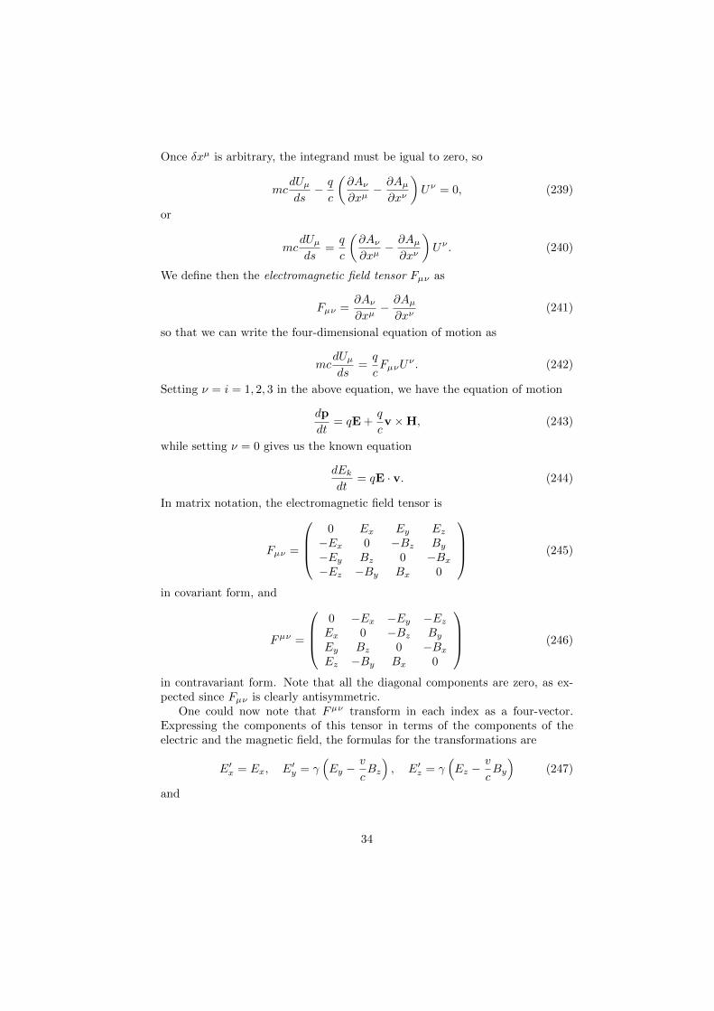
In matrix notation, the electromagnetic field tensor is
Fµν =
0 Ex Ey Ez−Ex 0 −Bz By−Ey Bz 0 −Bx−Ez −By Bx 0
(245)
in covariant form, and
Fµν =
0 −Ex −Ey −EzEx 0 −Bz ByEy Bz 0 −BxEz −By Bx 0
(246)
in contravariant form. Note that all the diagonal components are zero, as ex-pected since Fµν is clearly antisymmetric.
One could now note that Fµν transform in each index as a four-vector.Expressing the components of this tensor in terms of the components of theelectric and the magnetic field, the formulas for the transformations are
E′x = Ex, E′y = γ(Ey −
v
cBz
), E′z = γ
(Ez −
v
cBy
)(247)
and
34
B′x = Bx, B′y = γ(By +
v
cEz
), B′z = γ
(Bz +
v
cEy
). (248)
As a particular case, if v c then
E′x = Ex, E′y = Ey −v
cBz, E′z = Ez −
v
cBy (249)
and
B′x = Bx, B′y = By +v
cEz, B′z = Bz +
v
cEy, (250)
which can be written as
E′ = E− 1
c×v (251)
and
B′ = B +1
cE× v (252)
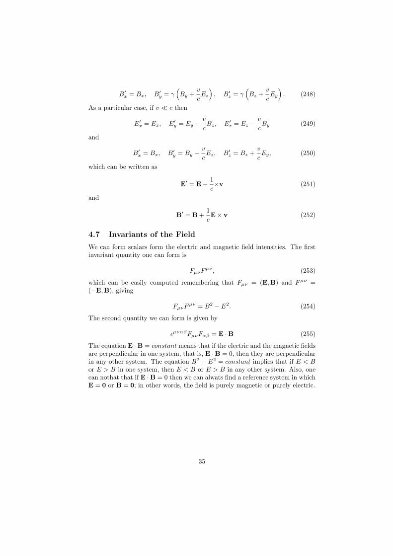
4.7 Invariants of the Field
We can form scalars form the electric and magnetic field intensities. The firstinvariant quantity one can form is
FµνFµν , (253)
which can be easily computed remembering that Fµν = (E,B) and Fµν =(−E,B), giving
FµνFµν = B2 − E2. (254)
The second quantity we can form is given by
εµναβFµνFαβ = E ·B (255)
The equation E ·B = constant means that if the electric and the magnetic fieldsare perpendicular in one system, that is, E ·B = 0, then they are perpendicularin any other system. The equation B2 − E2 = constant implies that if E < Bor E > B in one system, then E < B or E > B in any other system. Also, onecan nothat that if E ·B = 0 then we can alwats find a reference system in whichE = 0 or B = 0; in other words, the field is purely magnetic or purely electric.
35

5 The Electromagnetic Field Equations
5.1 The First Pair of Maxwell’s Equations
We already know that
B = ∇×A, E = −1
c
∂A
∂t−∇φ, (256)
so, using the fact that ∇× (∇f) = 0 for all scalar function f , we have
∇×E = −1
c
∂(∇×A)
∂t−∇× (∇φ) = −1
c
∂(∇×A)
∂t(257)
and now using the fact that ∇ · (∇×V) = 0 for all vector field V gives us
∇ ·B = ∇ · (∇×A) = 0, (258)
and these equations are the first pair of Maxwells equations, which are homo-geneous. In gour-dimensional notation, let us first remember that
Fµν = ∂µAν − ∂νAµ, (259)
so that
∂ρFµν+∂µFνρ+∂νFρµ = ∂ρ∂µAν−∂ρ∂νAµ+∂µ∂νAρ−∂µ∂ρAν+∂ν∂ρAµ−∂ν∂µAρ = 0(260)
since the derivatives commute. The quantity ∂ρFµν + ∂µFνρ + ∂νFρµ is anti-symmetric in all three indices, and the only non zero components are those with
µ 6= ν 6= ρ, so they form the set of four equations, which are ∇×E = 1c∂(∇×A)
∂tand ∇ ·B = 0.
5.2 The Four-dimensional Current Vector and Equationof Continuity
The charge density ρ = ρ(x, y, z, t) is defined so that ρdV is the charge containedin the volume dV , which allows us to treat charge as a continuously distributedquantity in the space. Charges, however, are pointlike, which allows us to write
ρ(r) =∑a
qaδ(r− ra), (261)
where ra is the radius vector of the charge qa. Multiplying now the quantitydQ = ρdV by dxµ gives us
dQdxµ = ρdV dxµ = ρdV dtdxµ
dt. (262)
Now, note that dQdxµis a four-vector, and hence the quantity ρdV dtdxµ/dtmust also be a four-vector. Once the quantity dV dt is a scalar, we conclude
36

that the quantty ρdxµ/dt is a four-vector. We define this vector as Jµ, whichis called current four-vector or four-current, and hence
Jµ = ρdxµ
dt, (263)
we can now evaluate
J0 = ρdx0
dt= ρ
d(ct)
dt= cρ (264)
and
J i = ρdxi
dt= ρv = j, (265)
where j is the current density vector. This way, we can write
Jµ = (cρ, j). (266)
Finally, the total charge, which is equal to∫ρdV , can also be written in four-
dimensional form as ∫ρdV =
1
c
∫J0dV =
1
c
∫JµdSµ (267)
taken over the four-dimensional hyperplane perpendicular to x0-axis.Let us now consider the change with time of the total charge, that is, the
quantity
∂
∂t
∫ρdV. (268)
First, one should note that the quantity of charge which passes in unit timethrough the element dS of the surface bounding our volume is given by ρv · dS,where v is the velocity of the charge where dS is located. The quantity ρv · dSis positive if charge leaves and negative otherwise. Remembering that j = ρv,we can write then
∂
∂t
∫ρdV = −
∮j · dS, (269)
where the integral on the right hand side extends over the whole boundary ofthe volume. This is called equation of continuity, in integral form. Applyingnow Gauss’ theorem on the right hand side gives us∫
j · dS =
∫(∇ · j)dV, (270)
and hence we have
∂
∂t
∫ρdV = −
∫(∇ · j)dV (271)
37

or ∫ (∂ρ
∂t+∇ · j
)dV = 0, (272)
which allows us to write
∂ρ
∂t+∇ · j = 0 (273)
since dV is arbitrary. This is the equation of continuity in differential form. Letus write now the above equation in the form
1
c
∂(cρ)
∂t+∂J1
∂x1+∂J2
∂x2+∂J3
∂x3= 0, (274)
and now note that cρ = J0 and ∂/∂(ct) = ∂/∂x0, so that we can write
∂µJµ = 0, (275)
which is the equation of continuity in four-dimensional form.
5.3 The Action Function for the Electromagnetic Field
Considering the electromagnetic field and the particles, the action function con-sists of three parts,
S = Sf + Sm + Smf , (276)
where Sf depends on the properties of the field itself, in the absence of charges,Sm depends only on the properties of the particle, and Smf depends on theinteraction between the particles and the field. This way, if there are manyparticles, the total action Sm is the sum of the actions for each free particle:
Sm = −∑
mc
∫ds. (277)
On the other hand, for a system of particles we will also have
Smf = −∑ q
c
∫Aµdx
µ. (278)
Now, we wish to stablish the form of the action Sf . In order to do that, let ususe the fact that the electromagnetic field satisfies the principle of superposition,which asserts that the field produced by a system of charges is the result of asimple composition of the fields produced by each of the particles individually.As we know, a linear differential equation has this property, and the linearcombination of any solution is also a solution. This way, under the integral signof Sf there must stand an expression quadratic in the field, and Sf must be theintegral of some function of the field tensor Fµν . In order to have a scalar asthe action, the quantity we look for is FµνF
µν , so that
38

Sf = a
∫FµνF
µνdxdydzdt, (279)
where a is a constant which depends on the choice of units. In the Gaussiansystem of units, we have a = −1/16π. If we define now
dΩ = cdtdxdydz, (280)
we have then
Sf = − 1
16πc
∫FµνF
µνdΩ, (281)
or, using the fact that FµνFµν = 2(B2 − E2),
Sf =1
8π
∫(E2 −B2)dV dt, (282)
and hence the total action for the fied and particles is
S = Sf + Sm + Smf = − 1
16πc
∫FµνF
µνdΩ−∑
mc
∫ds−
∑ q
c
∫Aµdx
µ.
(283)
5.4 The Second Pair of Maxwell’s Equations
In the expression (283) for the action function, we can introduce the currentfour-vector. In place of the point charges q, let us introduce the continuousdistribution of charge with density ρ, and write this term as
−1
c
∫ρAµdx
µdV, (284)
replacing the sum by an integral. We can rewrite this as
−1
c
∫ρdxµ
dtAµdV dt, (285)
or simply
− 1
c2
∫AµJ
µdΩ. (286)
The action then will be of the form
S = − 1
16πc
∫FµνF
µνdΩ−∑
mc
∫ds−
∑ 1
c2
∫AµJ
µdΩ. (287)
Now, note that the variation of the term −∑mc∫ds− is clearly zero, and so,
using the fact that FµνδFµν = FµνδFµν , we have
39

δS = −∫ (
1
8πcFµνδFµν +
1
c2δAµJ
µ
)dΩ = 0. (288)
Using now Fµν = ∂µAν − ∂νAµ gives us
δS = −∫ (
1
8πcFµν∂µδAν −
1
8πcFµν∂νδAµ +
1
c2δAµJ
µ
)dΩ = 0. (289)
We can now interchange the indices µ and ν in the expression Fµν∂µδAν andthen replacing Fµν by −F νµ, which gives us
δS = −∫ (− 1
4πcFµν∂νδAµ +
1
c2δAµJ
µ
)dΩ = 0. (290)
Integrating by parts the first term of this integral, remembering that the limitsof integration are infinity, where the field is zero, gives us the expression
δS = −∫ (
1
4πc∂νFµν +
1
c2Jµ)δAµdΩ = 0. (291)
or simply
−1
c
∫ (1
4π∂νFµν +
1
cJµ)δAµdΩ = 0. (292)
Since δAµ is arbitrary, its coefficients must be zero, so that we have
∂νFµν = −4π
cJµ, (293)
which is a set of four equations. If we set µ = 1 then we have the equation
∂Bz∂y− ∂By
∂z− 1
c
∂Ex∂t
=4π
cJx, (294)
and similarly if i = 2, 3, so that, in vector equation, we have
∇×B =1
c
∂E
∂t+
4π
cJ. (295)
On the other hand, If µ = 0, we have
∇ ·E = 4πρ, (296)
and these equations are called the second pair of Maxwell’s equations, or the in-homogeneous pair. It is easy to obtain the continuity equation from the Maxwellequations. Taking the divergence of equation (295), gives us
∇ · (∇×B) =1
c
∂(∇ ·E)
∂t+
4π
c(∇ · J). (297)
Once ∇ · (∇×B) = 0 and ∇ ·E = 4πρ, we have then
40

0 =1
c
∂(4πρ)
∂t+
4π
c(∇ · J), (298)
or simply
∇ · J +∂ρ
∂t= 0, (299)
which is the equation of continuity.
5.5 Energy Density
Let us consider the equations
∇×E = −1
c
∂B
∂t, ∇×B =
1
c
∂E
∂t+
4π
cj, (300)
multiply respectively by B and E and combine them, getting
B · (∇×E)−E · (∇×B) = −1
cB · ∂B
∂t− 1
cE · ∂E
∂t+
4π
cj ·E, (301)
and, using the formula ∇ · (a× b) = b · ∇ × a− a · ∇b, we can write
∇ · (E×B) = −4π
cj ·E− 1
2c
∂
∂t(E2 +B2), (302)
or simply
∂W
∂t= −j ·E−∇ · S, (303)
where the Poynting vector S is defined as
S =c
4πE×B (304)
and the energy density W as
W =E2 +B2
8π, (305)
which is the energy per unit volume of the field.
5.6 Energy-momentum tensor of the Electromagnetic Field
Consider a system whose action integral is
S =
∫Λ (q, ∂µq) dV dt =
1
c
∫ΛdΩ, (306)
where Λ is a function of q and their first derivatives. The integral∫
ΛdV is theLagrangian of the system, so that Λ can be interpreted as Lagrangian density.The equations of motion are obtained by varying S:
41

δS =1
c
∫ (∂Λ
∂qδq +
∂Λ
∂(∂µq)δ(∂µq)
)dΩ (307)
or
δS =1
c
∫ [∂Λ
∂qδq + ∂µ
(∂Λ
∂(∂µq)δq
)− δq∂µ
∂Λ
∂(∂µq)
]dΩ = 0. (308)
The term ∫∂µ
(∂Λ
∂(∂µq)δq
)dΩ (309)
vanishes, and by arbitrarity of dΩ and δq, the equation of motion is then
∂Λ
∂q− ∂µ
∂Λ
∂(∂µq)= 0. (310)
Write now
∂Λ
∂xµ=∂Λ
∂q
∂q
∂xµ+
∂Λ
∂(∂νq)
∂(∂νq)
∂xµ, (311)
and, using the equation of motion and the fact that ∂ν∂µq = ∂µ∂νq, we have
∂Λ
∂xµ=
∂
∂xν
(∂Λ
∂(∂νq)
)∂µq +
∂Λ
∂(∂νq)
∂(∂µq)
∂xν=
∂
∂xν
(∂µq
∂Λ
∂(∂νq)
). (312)
Also, we can write
∂Λ
∂xµ= δνµ
∂Λ
∂xν, (313)
and hence, if we define
T νµ = ∂µq∂Λ
∂(∂νq)− δνµΛ, (314)
then we can write
∂T νµ∂xν
= 0. (315)
We wish to apply now these relations to the electromagnetic field. First of all,remember that for the electromagnetic field we have
Λ = − 1
16πFνρF
νρ, (316)
so, using relation (314), the tensor of the electromagnetic field is
42

T νµ =∂Aρ∂xµ
∂Λ
∂(∂Aρ∂xν
) − δνµΛ, (317)
which gives, after finding the variation δΛ,
T νµ = − 1
4π
∂Aρ∂xµ
F νρ +1
16πδνµFρσF
ρσ, (318)
or, in contravariant form,
Tµν = − 1
4π
∂Aρ∂xµ
F νρ +1
16πgµνFρσF
ρσ, (319)
which is not, however, a symmetric tensor, so that we add the quantity
1
4π
∂Aµ
∂xρF νρ =
1
4π
∂
∂xρ(AµF νρ), (320)
and hence we have the final expression for the energy-momentum tensor of theelectromagnetic field,
Tµν =1
4π
(−FµρF νρ +
1
4gµνFρσF
ρσ
), (321)
which is symmetric and whose trace Tµµ = 0.
43

References
[1] Landau, Mario. Classical Theory of Fields. Addison Wesley, Massachusetts,5nd edition, 1989.
[2] Charap, John M. Covariant Electrodynamics, A Concise Guide. Johns Hop-kins, USA, 2011.
44