Department of Science and Technology Institutionen för teknik och naturvetenskap Linköping University Linköpings Universitet SE-601 74 Norrköping, Sweden 601 74 Norrköping

LiU-ITN-TEK-A--08/065--SE

Relationships between ImagePopularity and Color Emotions

in Image Retrieval SystemsFredrik Stenerfelt

2008-05-13

LiU-ITN-TEK-A--08/065--SE

Relationships between ImagePopularity and Color Emotions

in Image Retrieval SystemsExamensarbete utfört i medieteknik

vid Tekniska Högskolan vidLinköpings universitet

Fredrik Stenerfelt

Handledare Reiner LenzExaminator Reiner Lenz

Norrköping 2008-05-13

Upphovsrätt

Detta dokument hålls tillgängligt på Internet – eller dess framtida ersättare –under en längre tid från publiceringsdatum under förutsättning att inga extra-ordinära omständigheter uppstår.

Tillgång till dokumentet innebär tillstånd för var och en att läsa, ladda ner,skriva ut enstaka kopior för enskilt bruk och att använda det oförändrat förickekommersiell forskning och för undervisning. Överföring av upphovsrättenvid en senare tidpunkt kan inte upphäva detta tillstånd. All annan användning avdokumentet kräver upphovsmannens medgivande. För att garantera äktheten,säkerheten och tillgängligheten finns det lösningar av teknisk och administrativart.

Upphovsmannens ideella rätt innefattar rätt att bli nämnd som upphovsman iden omfattning som god sed kräver vid användning av dokumentet på ovanbeskrivna sätt samt skydd mot att dokumentet ändras eller presenteras i sådanform eller i sådant sammanhang som är kränkande för upphovsmannens litteräraeller konstnärliga anseende eller egenart.

För ytterligare information om Linköping University Electronic Press seförlagets hemsida http://www.ep.liu.se/

Copyright

The publishers will keep this document online on the Internet - or its possiblereplacement - for a considerable time from the date of publication barringexceptional circumstances.

The online availability of the document implies a permanent permission foranyone to read, to download, to print out single copies for your own use and touse it unchanged for any non-commercial research and educational purpose.Subsequent transfers of copyright cannot revoke this permission. All other usesof the document are conditional on the consent of the copyright owner. Thepublisher has taken technical and administrative measures to assure authenticity,security and accessibility.

According to intellectual property law the author has the right to bementioned when his/her work is accessed as described above and to be protectedagainst infringement.

For additional information about the Linköping University Electronic Pressand its procedures for publication and for assurance of document integrity,please refer to its WWW home page: http://www.ep.liu.se/

© Fredrik Stenerfelt

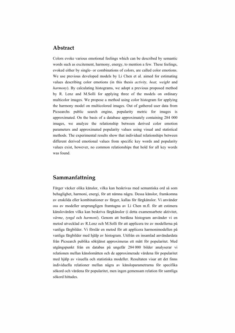
Abstract

Colors evoke various emotional feelings which can be described by semantic words such as excitement, harmony, energy, to mention a few. These feelings, evoked either by single- or combinations of colors, are called color emotions. We use previous developed models by Li Chen et al. aimed for estimating values describing color emotions (in this thesis activity, heat, weight and harmony). By calculating histograms, we adopt a previous proposed method by R. Lenz and M.Solli for applying three of the models on ordinary multicolor images. We propose a method using color histogram for applying the harmony model on multicolored images. Out of gathered user data from Picsearchs public search engine, popularity metric for images is approximated. On the basis of a database approximately containing 284 000 images, we analyze the relationship between derived color emotion parameters and approximated popularity values using visual and statistical methods. The experimental results show that individual relationships between different derived emotional values from specific key words and popularity values exist, however, no common relationships that hold for all key words was found.

Sammanfattning

Färger väcker olika känslor, vilka kan beskrivas med semantiska ord så som behaglighet, harmoni, energi, för att nämna några. Dessa känslor, framkomna av enskilda eller kombinationer av färger, kallas för färgkänslor. Vi använder oss av modeller ursprungligen framtagna av Li Chen m.fl. för att estimera känslovärden vilka kan beskriva färgkänslor (i detta examensarbete aktivitet, värme, tyngd och harmoni). Genom att beräkna histogram använder vi en metod utvecklad av R.Lenz och M.Solli för att applicera tre av modellerna på vanliga färgbilder. Vi förslår en metod för att applicera harmonimodellen på vanliga färgbilder med hjälp av histogram. Utifrån en insamlad användardata från Picsearch publika söktjänst approximeras ett mått för popularitet. Med utgångspunkt från en databas på ungefär 284 000 bilder analyserar vi relationen mellan känslomåtten och de approximerade värdena för popularitet med hjälp av visuella och statistiska modeller. Resultaten visar att det finns individuella relationer mellan några av känsloparametrarna för specifika sökord och värdena för popularitet, men ingen gemensam relation för samtliga sökord hittades.

Table of Content

CHAPTER 1.............................................................................................................................- 1 - INTRODUCTION .....................................................................................................................- 1 - 1.1 PROBLEM DESCRIPTION ...................................................................................................- 1 - 1.2 THE TASK AT HAND .........................................................................................................- 1 - 1.3 REPORT OUTLINE .............................................................................................................- 2 -

CHAPTER 2.............................................................................................................................- 3 - THEORETICAL BACKGROUND................................................................................................- 3 - 2.1 COLOR SPACES ................................................................................................................- 3 - 2.2 RGB COLOR SPACE..........................................................................................................- 3 - 2.3 CIELAB ...........................................................................................................................- 4 - 2.4 OTHER COLOR SPACES ....................................................................................................- 5 - 2.5 CONVERTING RGB TO CIELAB......................................................................................- 5 -

CHAPTER 3.............................................................................................................................- 7 - IMAGE DATABASES................................................................................................................- 7 - 3.1 CONTENT-BASED IMAGE RETRIEVAL ..............................................................................- 7 -

3.1.1 An overview of a simple CBIR-system ...................................................................... - 7 - 3.2 IMAGE FEATURES.............................................................................................................- 8 -

3.2.1 Color .......................................................................................................................... - 8 - 3.2.2 Color histogram ......................................................................................................... - 9 - 3.2.3 Dominant colors ...................................................................................................... - 10 -

3.3 SIMILARITY MEASURES...................................................................................................- 10 -

CHAPTER 4...........................................................................................................................- 11 - COLOR EMOTIONS ...............................................................................................................- 11 - 4.1 HUMANS EMOTIONAL RESPONSE .................................................................................- 11 - 4.2 COLOR EMOTION MODELS............................................................................................- 11 - 4.3 A COLOR HARMONY MODEL .......................................................................................- 13 -

CHAPTER 5...........................................................................................................................- 16 - METHODS ............................................................................................................................- 16 - 5.1 HISTOGRAM ...................................................................................................................- 16 - 5.2 APPLYING THE COLOR EMOTION MODEL TO IMAGES .................................................- 16 - 5.3 APPLYING THE COLOR HARMONY MODEL TO IMAGES ................................................- 17 - 5.4 USER DATA ....................................................................................................................- 18 - 5.5 THE DATABASE..............................................................................................................- 19 - 5.6 ANALYZING THE DATA .................................................................................................- 19 -

5.6.1 Geo Analytics Visualization (GAV) ........................................................................ - 19 - 5.6.2 Matlab ..................................................................................................................... - 20 - 5.6.3 Correlation............................................................................................................... - 21 - 5.6.4 Least Square Error Method ..................................................................................... - 22 - 5.6.5 The strength of the correlation................................................................................. - 22 -

5.6.5 Polynomial Regression ............................................................................................ - 23 -

CHAPTER 6...........................................................................................................................- 24 - RESULTS ...............................................................................................................................- 24 - 6.1 VISUAL ANALYSIS USING GEO ANALYTICS VISUALIZATION (GAV) ...........................- 24 -

6.1.1 Andy Warhol ........................................................................................................... - 24 - 6.1.2 Beach........................................................................................................................ - 24 - 6.1.3 Flower ...................................................................................................................... - 25 - 6.1.4 Garden ..................................................................................................................... - 25 -

6.2 VISUAL ANALYSIS USING MATLAB .............................................................................- 26 - 6.2.1 Activity.................................................................................................................... - 26 - 6.2.2 Weight ..................................................................................................................... - 27 - 6.2.3 Heat ......................................................................................................................... - 28 - 6.2.4 Harmony ................................................................................................................. - 29 -

6.3 LINEAR REGRESSION .....................................................................................................- 30 - 6.3 POLYNOMIAL REGRESSION............................................................................................- 32 -

CHAPTER 7...........................................................................................................................- 33 - DISCUSSION AND FUTURE WORK .......................................................................................- 33 - 7.1 DISCUSSION ...................................................................................................................- 33 - 7.2 FUTURE WORK...............................................................................................................- 34 -

GLOSSARY............................................................................................................................- 36 -

ACKNOWLEDGMENTS .........................................................................................................- 36 -

BIBLIOGRAPHY.....................................................................................................................- 37 -

APPENDIX A ........................................................................................................................- 39 - COLOR SCIENCE ..................................................................................................................- 39 - LIGHT SOURCES ...................................................................................................................- 39 - OBJECTS ...............................................................................................................................- 41 - COLOR STIMULI ...................................................................................................................- 41 - HUMAN COLOR VISION ......................................................................................................- 42 -

APPENDIX B .........................................................................................................................- 43 -

APPENDIX C ........................................................................................................................- 44 -

- 1 -

Chapter 1

Introduction Extracting image features has been, and still is, a very useful way of concisely characterizing images to allow efficient image retrieval. However, most content-based image retrieval systems are not taking high-level semantic information into account, for instance feelings. Recently, scientists at the Department of Science and Technology at Linköping University have started to investigate color-based emotion-related concepts in image retrieval and image classification. This study will adopt parts of their research and extend the scope to involve user related data.

1.1 Problem description Image retrieval system distributors like Picsearch are interested in displaying images that match both the user’s query and their expectations. To increase the probability that the query returns relevant and interesting images to the user, it is desirable to display images which users might find attractive. The most straightforward procedure is to display the images that are frequently clicked (selected) by users. This method will cause problems when new images, having zero clicks, are added to the database. It is therefore desirable to use for instance image analysis for predicting popularity values when the images are added to the database. Sorting and displaying the resulting images by an estimated popularity value will give the user a more meaningful result.

1.2 The task at hand The aim with this work is to analyze relationships and connections between derived color emotion features and the popularity measurements, if there are any, for color images included in Picsearchs public image retrieval system. Around 284 000 color images with corresponding user data received from Picsearch will be analyzed during this thesis. A concept for applying the color emotion models proposed by Li-Chen et. al. [14][17], described in section 4, on ordinary color images will be investigated in order to extract emotion-related image features. Together with the user data we will try to gain a better understanding of relationships and connections in the data set. A hypothetical idea is to generate a method that is able to estimate the popularity of an arbitrary image out of its color emotion values. To be realistic, this might seem like a utopia since there are a lot more factors other than colors involved in defining popular images.

- 2 -

1.3 Report outline This thesis report contains 7 chapters. A theoretical background is briefly covered in chapter 2 to chapter 4. The fundamentals of color science are discussed in chapter 2. Chapter 3 contains material about content-based image retrieval systems and image databases. Color emotions are discussed in chapter 4, completing the theoretical part of the thesis. The contributions of the thesis are presented in chapter 5 to chapter 7. The implementation and extraction of color-based emotion features and the structure of the database are presented in chapter 5. In chapter 6, the visual and mathematical results are presented. Finally, conclusions and ideas about future work are presented in chapter 7.

- 3 -

Chapter 2

Theoretical background

2.1 Color Spaces The color spectrum of the light reaching the retina of the eye contain several different wave lengths, see appendix A for more details. The human visual system maps these spectra onto a lower three dimensional space (three cones). In a practical sense we have to do the same thing when describing light or colors mathematically, in fact most color spaces are based on a three-dimensional description (e.g. RGB and CIELAB).

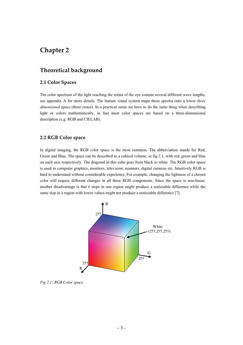
2.2 RGB Color space In digital imaging, the RGB color space is the most common. The abbreviation stands for Red, Green and Blue. The space can be described as a cubical volume, se fig 2.1, with red, green and blue on each axis respectively. The diagonal in this cube goes from black to white. The RGB color space is used in computer graphics, monitors, television, scanners, digital cameras etc. Intuitively RGB is hard to understand without considerable experience. For example, changing the lightness of a chosen color will require different changes in all three RGB components. Since the space is non-linear, another disadvantage is that k steps in one region might produce a noticeable difference while the same step in a region with lower values might not produce a noticeable difference [7].

Fig 2.1: RGB Color space

- 4 -

2.3 CIELAB CIELAB, or more correctly CIE L*a*b* was proposed by the CIE association in 1976. It is a device independent uniform color space, the Euclidean distance between two points in the space is taken to

be a measure of their color difference ( *abEΔ or *

uvEΔ ). CIELAB has become almost standard for

color specification and difference measurement. CIELAB is derived from the CIEXYZ color space, the X, Y and Z values are defined as:

∫=

∫=

∫=

∫=

λ λλλ

λλλ λλ

λλλ λλ

λλλ λλ

dyEk

dzSEkZ

dySEkY

dxSEkX

)()(

100

)()()(

)()()(

)()()(

(2.1)

where E( λ ) is the spectral power distribution of the light source, S( λ ) is the spectral reflectance of

a reflective object, )(λx , )(λy and )(λz are the color matching functions of the CIE Standard

Colorimetric Observer, k is a normalization factor.

If ≥nnn Z

ZYY

XX ,, 0.008857, the L*, a* and b* values are then derived as,

⎟⎟⎠

⎞⎜⎜⎝

⎛−=

⎟⎟⎠

⎞⎜⎜⎝

⎛−=

−=

33

33

3

200*

500*

16116*

nn

nn

n

ZZ

YYb

YY

XXa

YYL

(2.2)

where Xn,Yn and Zn are the CIEXYZ coordinates of an desired white point. When ≤nnn Z

ZYY

XX ,,

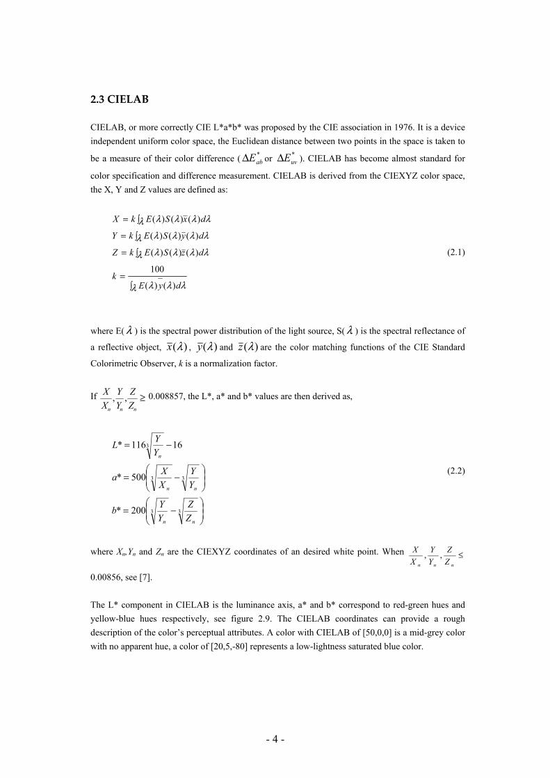
0.00856, see [7]. The L* component in CIELAB is the luminance axis, a* and b* correspond to red-green hues and yellow-blue hues respectively, see figure 2.9. The CIELAB coordinates can provide a rough description of the color’s perceptual attributes. A color with CIELAB of [50,0,0] is a mid-grey color with no apparent hue, a color of [20,5,-80] represents a low-lightness saturated blue color.

- 5 -

Figure 2.9 CIEL*a*b* color space [7].

2.4 Other Color Spaces

sRGB is a standard Red Green Blue color space developed by HP and Microsoft special aiming for display devices. Since sRGB serves as a best guess for how another person's monitor produces color, it has become the standard color space for displaying images on the internet. sRGB's color gamut encompasses only 35% of the visible colors specified by CIE. Although sRGB results in one of the narrowest gamut of any working space, sRGB's gamut is still considered broad enough for most color applications [2] [19] [27]. HSL represents several similar colour spaces, alternative names include HSI (intensity), HSV (value), HCI (chroma / colourfulness), HVC, TSD (hue saturation and darkness) to name a few. Most of these colour spaces are linear transforms from RGB and are therefore device dependent and non–linear [2].

2.5 Converting RGB to CIELAB It is often desirable to convert coordinates from one color space to another, especially converting a non-uniform color space to a uniform color space. RGB is the most common color space for digital images, but as mentioned earlier, CIELAB is to prefer when measuring color differences. The conversion from RGB to CIELAB is done in two steps; first the RGB vectors are converted to CIEXYZ coordinates using a linear transformation. In the next step the CIEXYZ coordinates are converted to CIELAB coordinates with help of a non-linear transformation.

- 6 -

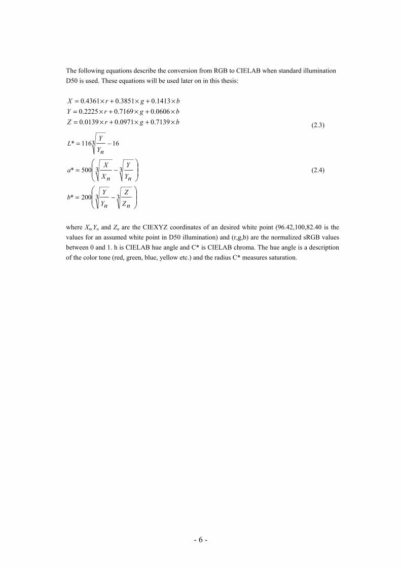
The following equations describe the conversion from RGB to CIELAB when standard illumination D50 is used. These equations will be used later on in this thesis:

bgrZbgrYbgrX

×+×+×=×+×+×=×+×+×=

7139.00971.00139.00606.07169.02225.01413.03851.04361.0

(2.3)

⎟⎟⎠

⎞⎜⎜⎝

⎛

⎟⎟⎠

⎞⎜⎜⎝

⎛

−=

−=

−=

33200*

33500*

163116*

nZ

Z

nY

Yb

nY

Y

nX

Xa

nY

YL

(2.4)

where Xn,Yn and Zn are the CIEXYZ coordinates of an desired white point (96.42,100,82.40 is the values for an assumed white point in D50 illumination) and (r,g,b) are the normalized sRGB values between 0 and 1. h is CIELAB hue angle and C* is CIELAB chroma. The hue angle is a description of the color tone (red, green, blue, yellow etc.) and the radius C* measures saturation.

- 7 -

Chapter 3

Image Databases This chapter describes techniques and applications of content-based image retrieval. The expansion of the World Wide Web has increased the information exchange tremendously. The very first image databases relied on text-based solutions when retrieving images. As the demands of accurate information and better retrievals have increased, the content itself in the image have become more and more interesting to use in retrieval. The following discussions will describe image retrieval systems in general but focus will be on color-based features.

3.1 Content-based Image Retrieval A Content-Based Image Retrieval (CBIR) system has to analyze both the content of the image as well as the user’s requirements in order to retrieve those images that are relevant for the user. The most popular modes are; search by association, target search and category search [9]. When a user makes a search by association he or she has no specific aims other than to find interesting images. The query can for example be a sketch or an example image. The result of the search can be manipulated interactively by reference feedback in order to improve the search. The purpose of the second category, target search, is to find a specific image, often used when the user has an example image in mind. The purpose of the third category, category search, is to retrieve an arbitrary image representing a specific category or class.

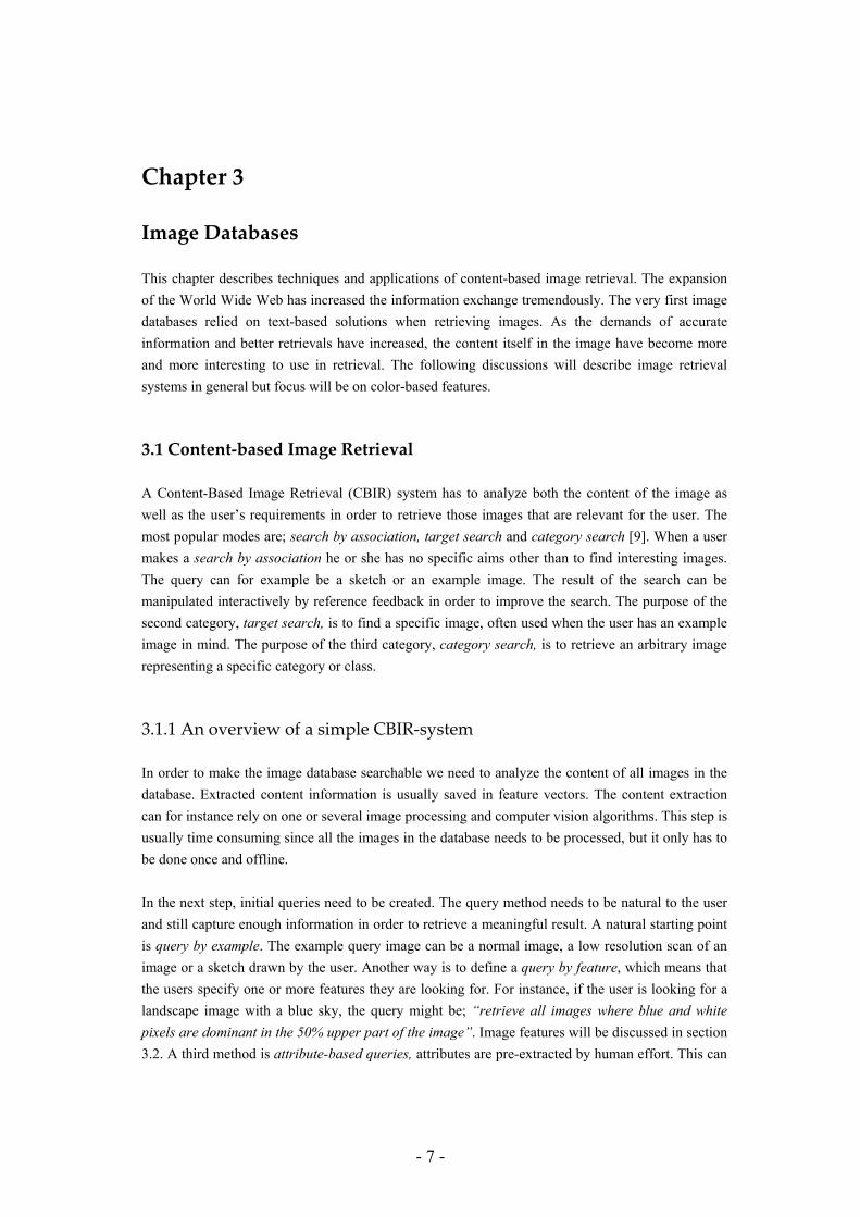
3.1.1 An overview of a simple CBIR-system In order to make the image database searchable we need to analyze the content of all images in the database. Extracted content information is usually saved in feature vectors. The content extraction can for instance rely on one or several image processing and computer vision algorithms. This step is usually time consuming since all the images in the database needs to be processed, but it only has to be done once and offline. In the next step, initial queries need to be created. The query method needs to be natural to the user and still capture enough information in order to retrieve a meaningful result. A natural starting point is query by example. The example query image can be a normal image, a low resolution scan of an image or a sketch drawn by the user. Another way is to define a query by feature, which means that the users specify one or more features they are looking for. For instance, if the user is looking for a landscape image with a blue sky, the query might be; “retrieve all images where blue and white pixels are dominant in the 50% upper part of the image”. Image features will be discussed in section 3.2. A third method is attribute-based queries, attributes are pre-extracted by human effort. This can

- 8 -

provide great abstractions since images contain a lot of information that is hard to summarize using just a few keywords. Nevertheless, like step one, features needs to be extracted in one way or another for matching with the database. The final step is the matching between the query and all images in the database. This step is done online and therefore it has to be very fast. Matching techniques will be discussed in section 3.3.

Figure 3.1: Overview of the basic concepts of CBIR-systems [9].

3.2 Image Features A wide definition of features is that they describe the content of an image, but rarely the complete content. Usually, different feature descriptors describe different content, for instance text, color, shapes or texture. When choosing a method for feature extraction the main idea is that the retrieval system should present similar images, i.e. similar according to user opinion.

3.2.1 Color Color is the most commonly used visual feature in image retrieval systems [9]. Typical color images taken by a digital camera contain pixel values in a three dimensional color vector space (grayscale images have only one channel and multi-spectral images can have more than three channels), i.e. we

- 9 -

can consider the color information as a three dimensional signal. The signals can be interpreted and modeled in different color spaces, for example RGB and CIE L*a*b* (as mentioned earlier). In image retrieval, no color space can be considered universal. Selecting a proper color space can be of great importance for the perceived accuracy of the image retrieval system. The most straightforward way to analyze the signal is by using multivariate probability density estimation methods such as histograms, color signatures, color moments and dominant colors.

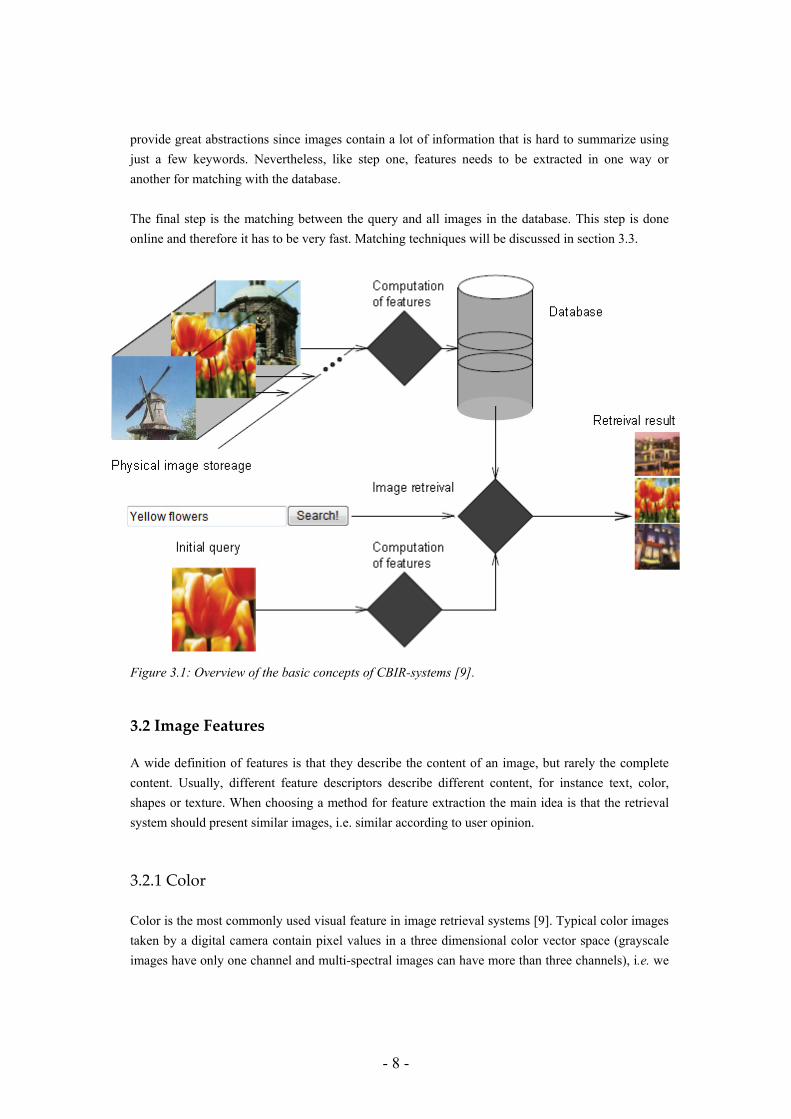
3.2.2 Color histogram Histograms are one of the most commonly used methods for measuring statistical properties of color images. A color histogram describes the probability of an arbitrary pixel value falling into a specific range of the data. It is easy to compute and is therefore a popular representation of color distribution. Data, in this case pixel values in an image, are divided into n regions or bins. The total numbers of

pixels in image I(x,y) of size YX × falling into each region is summed up and the histogram is normalized, i.e. divided by the total number of pixels in the image:

{∑−

=∑−

==

1 1

01

)(X

ox

Y

yXYmch 1 if I(x,y) in bin m, 0 otherwise } [7] (3.1)

Figure 3.2: a) An RGB image with its corresponding intensity histogram (R+G+B). b) The R-channel of the same image with its corresponding histogram for the red channel [19]. When computing histograms, two things need to be taken into consideration, the bin width and bin locations. Different numbers of bins will change the accuracy of the histogram. Decreasing the numbers of bins will decrease the accuracy of the color distribution. Taking bin locations into

- 10 -

consideration may be important when for instance dealing with special collections of images dominated by certain colors.

3.2.3 Dominant colors From figure 3.2 we can see that some bins are more frequently represented than others, a peak from the bright sky and the ocean can be seen to the right while a peak from the dark red and green cliffs can be seen to the left in the histogram. These bins are referred to as dominant colors and often they are efficient for characterizing the color content of an image. A better representation with less loss of color information can be achieved by clustering algorithms. (Clustering is not covered in this thesis. For interested readers we refer to [11]).

3.3 Similarity measures Measuring similarity between images can be done by measuring the distance between image features in the feature space. A short distance in feature space suggests that two images are similar. However, selecting a distance algorithm is usually a trade-off between complexity and computational time, and we can seldom perfectly resemble the human perceptual system. The computational time is usually a critical factor since many distances are calculated online. Several distance measures have been proposed, a commonly used is the Minkowski distance given by,

∑=

−=n

ipp

iliklkMD1

1)||(),( (3.2)

where n is the number of bins, k and l are feature vectors. Setting p=2 in the previous equation gives us the Euclidean distance as follow,

∑=

−=n

i iliklkED1

2)(),( (3.3)

where n is the number of bins, k and l are feature vectors More distances can be found in [9].

- 11 -

Chapter 4

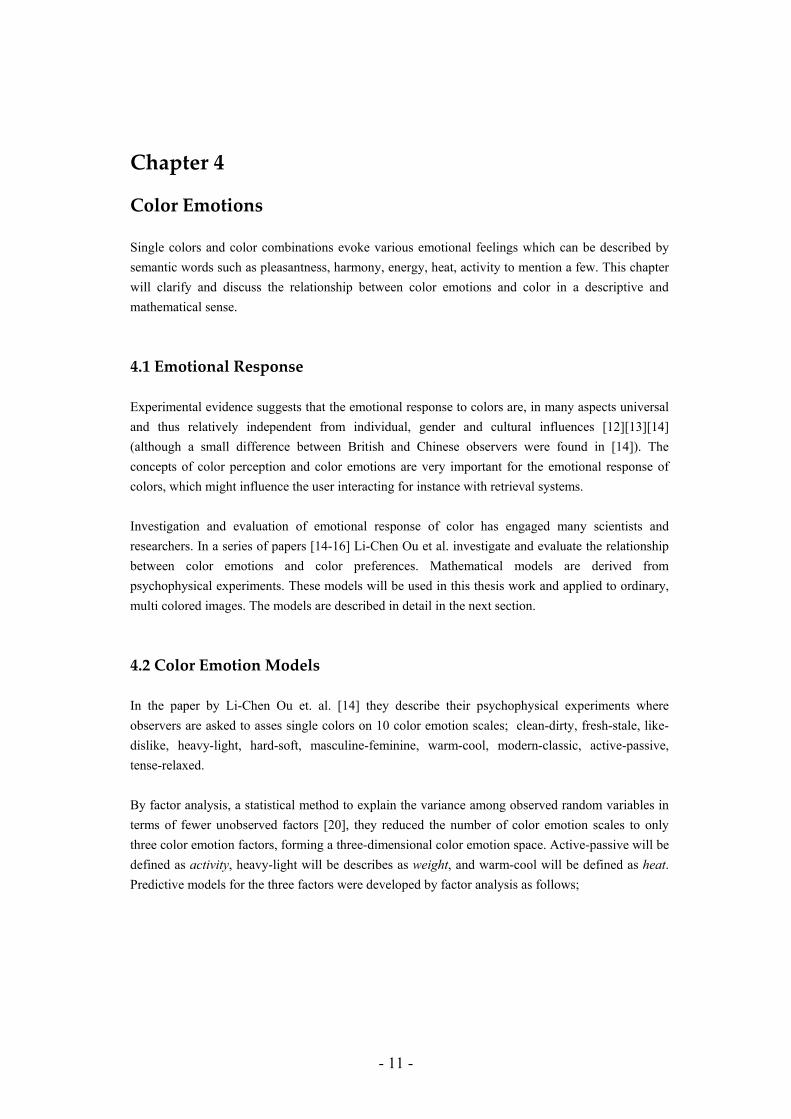
Color Emotions Single colors and color combinations evoke various emotional feelings which can be described by semantic words such as pleasantness, harmony, energy, heat, activity to mention a few. This chapter will clarify and discuss the relationship between color emotions and color in a descriptive and mathematical sense.

4.1 Emotional Response Experimental evidence suggests that the emotional response to colors are, in many aspects universal and thus relatively independent from individual, gender and cultural influences [12][13][14] (although a small difference between British and Chinese observers were found in [14]). The concepts of color perception and color emotions are very important for the emotional response of colors, which might influence the user interacting for instance with retrieval systems. Investigation and evaluation of emotional response of color has engaged many scientists and researchers. In a series of papers [14-16] Li-Chen Ou et al. investigate and evaluate the relationship between color emotions and color preferences. Mathematical models are derived from psychophysical experiments. These models will be used in this thesis work and applied to ordinary, multi colored images. The models are described in detail in the next section.

4.2 Color Emotion Models In the paper by Li-Chen Ou et. al. [14] they describe their psychophysical experiments where observers are asked to asses single colors on 10 color emotion scales; clean-dirty, fresh-stale, like-dislike, heavy-light, hard-soft, masculine-feminine, warm-cool, modern-classic, active-passive, tense-relaxed. By factor analysis, a statistical method to explain the variance among observed random variables in terms of fewer unobserved factors [20], they reduced the number of color emotion scales to only three color emotion factors, forming a three-dimensional color emotion space. Active-passive will be defined as activity, heavy-light will be describes as weight, and warm-cool will be defined as heat. Predictive models for the three factors were developed by factor analysis as follows;

- 12 -

Color activity 21

4.1

2)17*(2)3*(2)50*(06.01.2⎥⎥⎦

⎤

⎢⎢⎣

⎡ −+−+−+−=

baL (4.1)

Color weight )100cos(45.0*)100(04.08.1 °−+−+−= hL (4.2)

Color heat )50cos(07.1*)(02.05.0 °−+−= hC (4.3)

⎟⎠⎞

⎜⎝⎛=

**

arctanba

h (4.4)

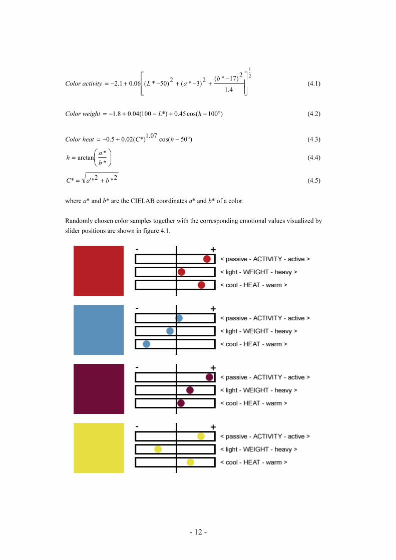
2*2'** baC += (4.5) where a* and b* are the CIELAB coordinates a* and b* of a color. Randomly chosen color samples together with the corresponding emotional values visualized by slider positions are shown in figure 4.1.

- 13 -

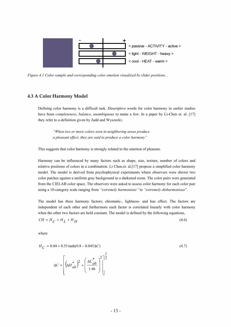
Figure 4.1 Color sample and corresponding color emotion visualized by slider positions. .

4.3 A Color Harmony Model Defining color harmony is a difficult task. Descriptive words for color harmony in earlier studies have been completeness, balance, unambiguous to name a few. In a paper by Li-Chen et. al. [17] they refer to a definition given by Judd and Wyszecki; “When two or more colors seen in neighboring areas produce a pleasant effect, they are said to produce a color harmony” This suggests that color harmony is strongly related to the emotion of pleasure. Harmony can be influenced by many factors such as shape, size, texture, number of colors and relative positions of colors in a combination. Li Chen.et. al.[17] propose a simplified color harmony model. The model is derived from psychophysical experiments where observers were shown two color patches against a uniform gray background in a darkened room. The color pairs were generated from the CIELAB color space. The observers were asked to assess color harmony for each color pair using a 10-category scale ranging from “extremely harmonious” to “extremely disharmonious”. The model has three harmony factors; chromatic-, lightness- and hue effect. The factors are independent of each other and furthermore each factor is correlated linearly with color harmony when the other two factors are held constant. The model is defined by the following equations,

HHLHCHCH ++= (4.6)

where

)045.08.0tanh(53.004.0 CCH Δ−+= (4.7)

( )21

2

46.1

*2*

⎥⎥⎥

⎦

⎤

⎢⎢⎢

⎣

⎡

⎟⎟

⎠

⎞

⎜⎜

⎝

⎛ Δ+Δ=Δ abC

abHC

- 14 -

LHLsumHLH Δ+= (4.8)

)029.0388.0tanh(54.028.0 sumLLsumH ++=

in which *2

*1 LL

sumL +=

)2.02tanh(15.014.0 LLH Δ+−+=Δ

in which *2

*1 LLL −=Δ

21 SYHSYHHH += (4.9)

⎪⎭

⎪⎬⎫

⎪⎩

⎪⎨⎧

⎥⎦

⎤⎢⎣

⎡

⎥⎥⎦

⎤

⎢⎢⎣

⎡ −°−

−°−=

°+−°+−−=

+−+=

+=

10

)90(exp

10

)90(exp

10

)8.12*22.0(

)902sin(07.0)50sin(14.008.0

)*5.02tanh(5.05.0

)(*

abhabhLYE

abhabhSH

abCCE

YESHCESYH

where CH is the color harmony score, LH is the lightness harmony score, HH is the hue

harmony score, abh is the CIELAB hue angle, *L is the lightness value, *abCΔ and *

abHΔ are the

CIELAB color difference values in chroma and hue, respectively.

The predicted values CH range from -1.24 to 1.39 on an interval scale. The smaller CH value the less harmonious the color pair would appear and vice versa.

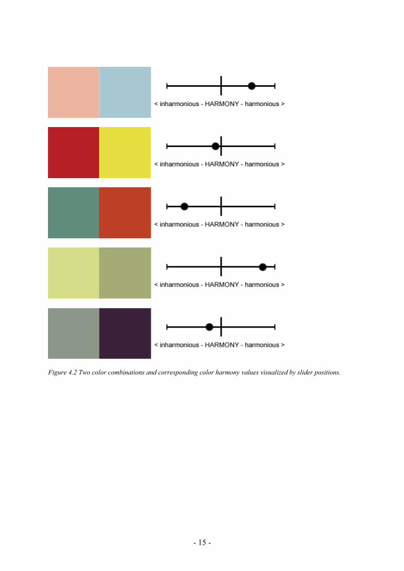
To ensure the general applicability of the model, tests using an independent psychophysical dataset accumulated by Gurar et al.[23] were implemented by Li Chen et al. The experiment was conducted under different experimental settings such as display media, color sample, light sources and carried out by 12 new observers with different cultural background. The experimental result agreed well with the harmony values predicted by equation 4.6. This suggests that the model can predict color harmony accurately under conditions that deviate from Li Chens’ study[17]. Randomly chosen combinations of color samples together with corresponding harmony values visualized by slider positions are shown in figure 4.2.

- 15 -

Figure 4.2 Two color combinations and corresponding color harmony values visualized by slider positions.

- 16 -

Chapter 5

Methods

5.1 Histogram We only consider ordinary color images with three channels, Red, Green and Blue. Using MATLAB, each channel is divided into eight equally spaced quantization levels, giving us totally 83 = 512 bins in each histogram. Histograms for all images in the database are saved in a matrix H of size 512×N , where N is the number of images. To keep the files manageable in size, the data is divided and stored in arrays of N = 1000 histograms.

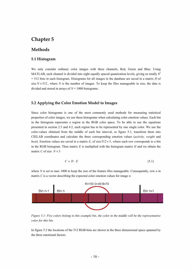
5.2 Applying the Color Emotion Model to Images Since color histograms is one of the most commonly used methods for measuring statistical properties of color images, we use these histograms when calculating color emotion values. Each bin in the histogram represents a region in the RGB color space. To be able to use the equations presented in section 2.5 and 4.2, each region has to be represented by one single color. We use the color-values obtained from the middle of each bin interval, se figure 5.1, transform them into CIELAB coordinates and calculate the three corresponding emotion values (activity, weight and heat). Emotion values are saved in a matrix E, of size 3512 × , where each row corresponds to a bin in the RGB histogram. Then matrix E is multiplied with the histogram matrix H and we obtain the matrix C of size 3×N EHC ⋅= (5.1) where N is set to max 1000 to keep the size of the feature files manageable. Consequently, row n in matrix C is a vector describing the expected color emotion values for image n.

Figure 5.1: Five colors belong to this example bin, the color in the middle will be the representative color for this bin. In figure 5.2 the locations of the 512 RGB-bins are shown in the three dimensional space spanned by the three emotional factors.

- 17 -

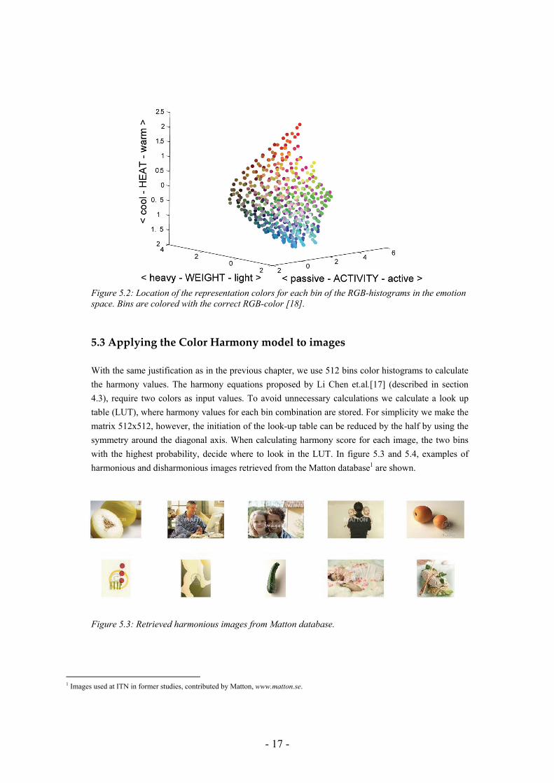
Figure 5.2: Location of the representation colors for each bin of the RGB-histograms in the emotion space. Bins are colored with the correct RGB-color [18].

5.3 Applying the Color Harmony model to images With the same justification as in the previous chapter, we use 512 bins color histograms to calculate the harmony values. The harmony equations proposed by Li Chen et.al.[17] (described in section 4.3), require two colors as input values. To avoid unnecessary calculations we calculate a look up table (LUT), where harmony values for each bin combination are stored. For simplicity we make the matrix 512x512, however, the initiation of the look-up table can be reduced by the half by using the symmetry around the diagonal axis. When calculating harmony score for each image, the two bins with the highest probability, decide where to look in the LUT. In figure 5.3 and 5.4, examples of harmonious and disharmonious images retrieved from the Matton database1 are shown.

Figure 5.3: Retrieved harmonious images from Matton database.

1 Images used at ITN in former studies, contributed by Matton, www.matton.se.

- 18 -

Figure 5.4: Retrieved disharmonious images from Matton database.

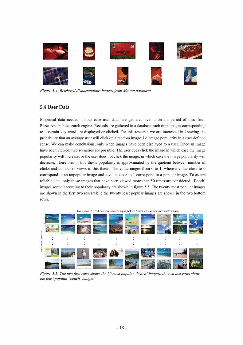
5.4 User Data Empirical data needed, in our case user data, are gathered over a certain period of time from Picsearchs public search engine. Records are gathered in a database each time images corresponding to a certain key word are displayed or clicked. For this research we are interested in knowing the probability that an average user will click on a random image, i.e. image popularity in a user defined sense. We can make conclusions, only when images have been displayed to a user. Once an image have been viewed, two scenarios are possible. The user does click the image in which case the image popularity will increase, or the user does not click the image, in which case the image popularity will decrease. Therefore, in this thesis popularity is approximated by the quotient between number of clicks and number of views in this thesis. The value ranges from 0 to 1, where a value close to 0 correspond to an unpopular image and a value close to 1 correspond to a popular image. To assure reliable data, only those images that have been viewed more than 50 times are considered. ‘Beach’ images sorted according to their popularity are shown in figure 5.5. The twenty most popular images are shown in the first two rows while the twenty least popular images are shown in the two bottom rows.

Figure 5.5: The two first rows shows the 20 most popular ‘beach’ images, the two last rows show the least popular ‘beach’ images.

- 19 -

5.5 The Database A part of this thesis work has been to extract and organize the data in order to be able analyze the data in an efficient way. The received data from Picsearch contains unsorted image files (approximate 234.000 images) and corresponding information files containing key words, references to the image files, number of views and number of clicks. The key words handled in this thesis are; Andy Warhol2, Beach, Flower and Garden. The database also contains the following keywords; Animal, Bald Eagle, Beastie Boys, Car, Cat, Claude Monet, Depeche Mode, Dog, Flower, Foo Fighters, Food, Fruit, Good Charlotte, Green Day, Lion, Love, Metallica, Snowpatrol, Weezer, Westlife. These are not analyzed since the number of images with more than 50 views is not enough to produce a reliable result. An explanation of the database structure can be found in appendix B.

5.6 Analyzing the Data There are arbitrary many ways to analyze data, for this thesis we are interested in analyzing the correlation between the estimation of popularity and the color emotion values previously calculated. We want to scan and analyze a large amount of data. The initial strategy is to visualize the information, to enable understanding of the data and find visual indication of correlations. Creating visualizations is fast and time efficient in order to describe the information, but in a scientific sense it is not an accurate and precise method for investigating correlation. Using different visual methods such as analyzing toolkits and MATLAB programming will help us during the analysis. In a second stage mathematical approval for the correlation will be gained, and the strength of the correlation estimated.

5.6.1 Geo Analytics Visualization (GAV) To get a basic understanding of the datasets we will initially carry out experiments using the Geo Analytics Visualization (GAV). GAV is a free component toolkit developed by Visual Information Technology and Applications (VITA) institution at Linköping University Campus Norrköping. It is aimed for dynamically exploring multivariate attributes simultaneously [21]. The data for each keyword are loaded from the database created in MATLAB trough an excel-sheet into GAV. The parameters we load are click, view, activity, weight, heat, harmony and popularity. The first and most straight forward experiment is to look at two parameters plotted against each

2 Andrew Warhola (August 6, 1928 – February 22, 1987), better known as Andy Warhol, was an American artist and a central figure in the movement known as Pop art. After a successful career as a commercial illustrator, Warhol became famous worldwide for his work as a painter and filmmaker.

- 20 -

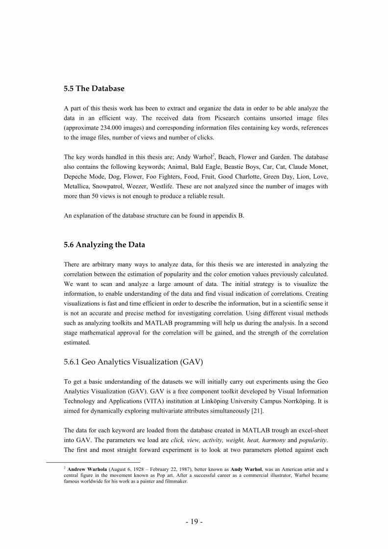
other in a 2D-coordinat system. The scatter matrix interface show us all parameters plotted versus each other, se figure 5.6.

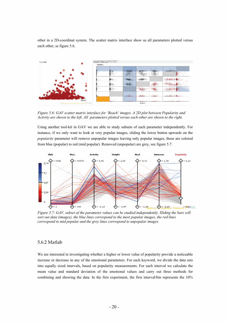
Figure 5.6: GAV scatter matrix interface for ‘Beach’ images. A 2D plot between Popularity and Activity are shown to the left. All parameters plotted versus each other are shown to the right. Using another tool-kit in GAV we are able to study subsets of each parameter independently. For instance, if we only want to look at very popular images, sliding the lower button upwards on the popularity parameter will remove unpopular images leaving only popular images, these are colored from blue (popular) to red (mid popular). Removed (unpopular) are grey, see figure 5.7.

Figure 5.7: GAV, subset of the parameter values can be studied independently. Sliding the bars will sort out data (images), the blue lines correspond to the most popular images, the red lines correspond to mid popular and the grey lines correspond to unpopular images.

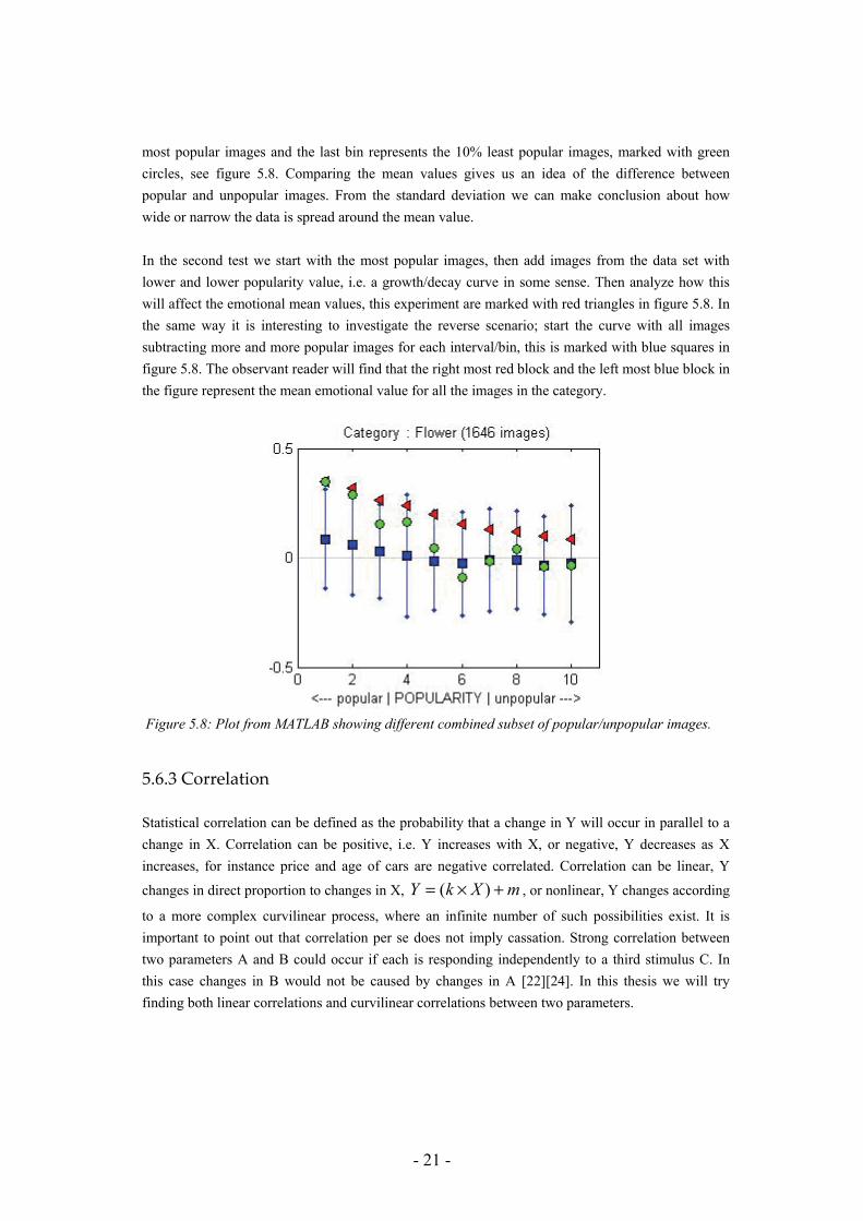
5.6.2 Matlab We are interested in investigating whether a higher or lower value of popularity provide a noticeable increase or decrease in any of the emotional parameters. For each keyword, we divide the data sets into equally sized intervals, based on popularity measurements. For each interval we calculate the mean value and standard deviation of the emotional values and carry out three methods for combining and showing the data. In the first experiment, the first interval/bin represents the 10%

- 21 -

most popular images and the last bin represents the 10% least popular images, marked with green circles, see figure 5.8. Comparing the mean values gives us an idea of the difference between popular and unpopular images. From the standard deviation we can make conclusion about how wide or narrow the data is spread around the mean value. In the second test we start with the most popular images, then add images from the data set with lower and lower popularity value, i.e. a growth/decay curve in some sense. Then analyze how this will affect the emotional mean values, this experiment are marked with red triangles in figure 5.8. In the same way it is interesting to investigate the reverse scenario; start the curve with all images subtracting more and more popular images for each interval/bin, this is marked with blue squares in figure 5.8. The observant reader will find that the right most red block and the left most blue block in the figure represent the mean emotional value for all the images in the category.

Figure 5.8: Plot from MATLAB showing different combined subset of popular/unpopular images.

5.6.3 Correlation Statistical correlation can be defined as the probability that a change in Y will occur in parallel to a change in X. Correlation can be positive, i.e. Y increases with X, or negative, Y decreases as X increases, for instance price and age of cars are negative correlated. Correlation can be linear, Y

changes in direct proportion to changes in X, mXkY +×= )( , or nonlinear, Y changes according

to a more complex curvilinear process, where an infinite number of such possibilities exist. It is important to point out that correlation per se does not imply cassation. Strong correlation between two parameters A and B could occur if each is responding independently to a third stimulus C. In this case changes in B would not be caused by changes in A [22][24]. In this thesis we will try finding both linear correlations and curvilinear correlations between two parameters.

- 22 -

5.6.4 Least Square Error Method The least square error method describes the correlation between two parameters with a straight line,

mXkY +⋅= , the linear regression line, see figure 5.10. Mathematically, the least square error method means that the constant variables k and m are to be decided so that the quadratic sum,

[ ]2)(∑ ⋅+− xkmy (5.2)

will be as small as possible. The following equations describe how to calculate k and m,

xkym ⋅−= (5.3)

where y and x are the mean values and

( )( )( )∑ −

∑ −−= 2

xx

yyxxk (5.4)

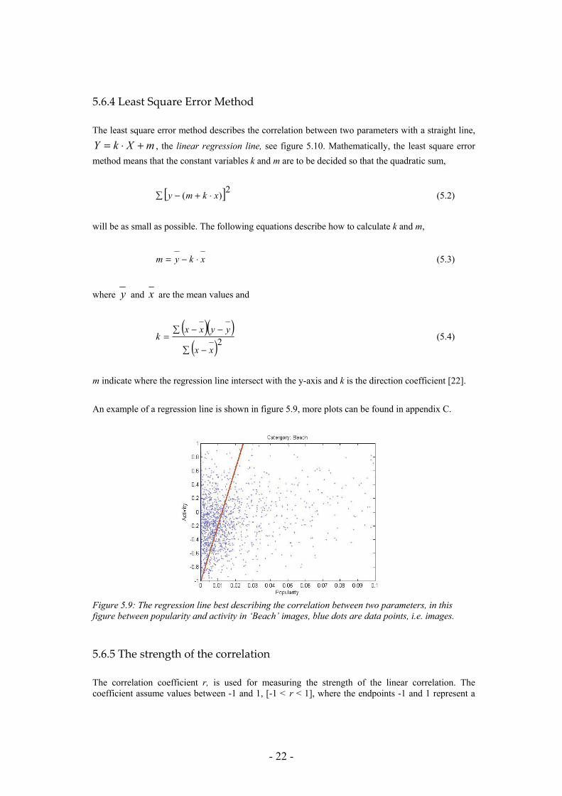
m indicate where the regression line intersect with the y-axis and k is the direction coefficient [22]. An example of a regression line is shown in figure 5.9, more plots can be found in appendix C.

Figure 5.9: The regression line best describing the correlation between two parameters, in this figure between popularity and activity in ‘Beach’ images, blue dots are data points, i.e. images.

5.6.5 The strength of the correlation The correlation coefficient r, is used for measuring the strength of the linear correlation. The coefficient assume values between -1 and 1, [-1 < r < 1], where the endpoints -1 and 1 represent a

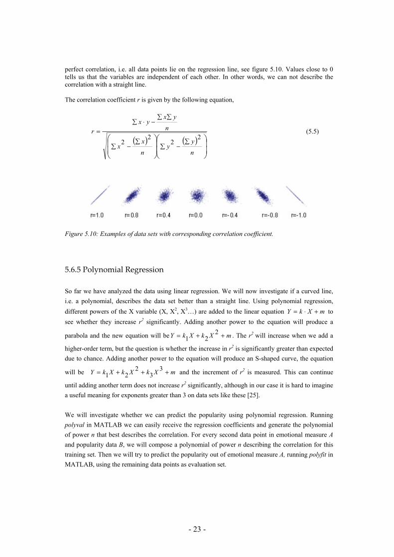
- 23 -

perfect correlation, i.e. all data points lie on the regression line, see figure 5.10. Values close to 0 tells us that the variables are independent of each other. In other words, we can not describe the correlation with a straight line. The correlation coefficient r is given by the following equation,

( ) ( )⎟⎟⎠

⎞⎜⎜⎝

⎛⎟⎟⎠

⎞⎜⎜⎝

⎛ ∑−∑

∑−∑

∑∑−∑ ⋅

=

n

yy

n

xx

n

yxyx

r2

22

2 (5.5)

Figure 5.10: Examples of data sets with corresponding correlation coefficient.

5.6.5 Polynomial Regression So far we have analyzed the data using linear regression. We will now investigate if a curved line, i.e. a polynomial, describes the data set better than a straight line. Using polynomial regression, different powers of the X variable (X, X2, X3…) are added to the linear equation mXkY +⋅= to see whether they increase r2 significantly. Adding another power to the equation will produce a

parabola and the new equation will be mXkXkY ++= 221 . The r2 will increase when we add a

higher-order term, but the question is whether the increase in r2 is significantly greater than expected due to chance. Adding another power to the equation will produce an S-shaped curve, the equation

will be mXkXkXkY +++= 33

221 and the increment of r2 is measured. This can continue

until adding another term does not increase r2 significantly, although in our case it is hard to imagine a useful meaning for exponents greater than 3 on data sets like these [25]. We will investigate whether we can predict the popularity using polynomial regression. Running polyval in MATLAB we can easily receive the regression coefficients and generate the polynomial of power n that best describes the correlation. For every second data point in emotional measure A and popularity data B, we will compose a polynomial of power n describing the correlation for this training set. Then we will try to predict the popularity out of emotional measure A, running polyfit in MATLAB, using the remaining data points as evaluation set.

- 24 -

Chapter 6

Results

6.1 Visual analysis using Geo Analytics Visualization (GAV) At first sight GAV seemed to be a proper tool for analyzing the data. During the first experiment, where parameters are plotted in 2D-coordinate system, the rough resolution combined with the amount of data points made it impossible to see any distinct indication of correlation between popularity and other parameters, see figure 5.4 in previous section. From these experiments we where not able to make any conclusions. Better understanding of the data set was achieved during the second experiment, where all the emotional parameters are plotted simultaneously and where we are able to change and restrict the parameter values individually.

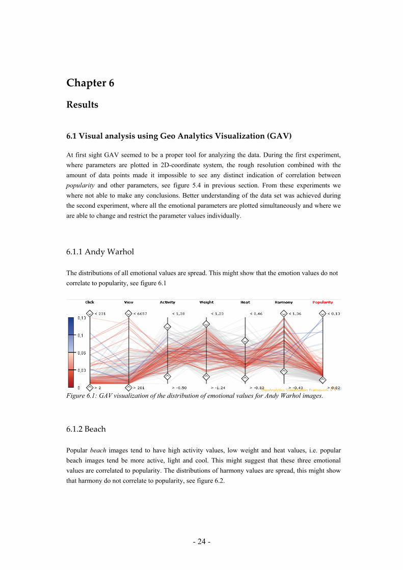
6.1.1 Andy Warhol The distributions of all emotional values are spread. This might show that the emotion values do not correlate to popularity, see figure 6.1

Figure 6.1: GAV visualization of the distribution of emotional values for Andy Warhol images.

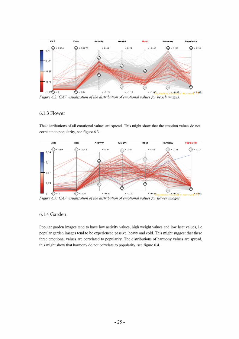
6.1.2 Beach Popular beach images tend to have high activity values, low weight and heat values, i.e. popular beach images tend be more active, light and cool. This might suggest that these three emotional values are correlated to popularity. The distributions of harmony values are spread, this might show that harmony do not correlate to popularity, see figure 6.2.

- 25 -

Figure 6.2: GAV visualization of the distribution of emotional values for beach images.

6.1.3 Flower The distributions of all emotional values are spread. This might show that the emotion values do not correlate to popularity, see figure 6.3.

Figure 6.3: GAV visualization of the distribution of emotional values for flower images.

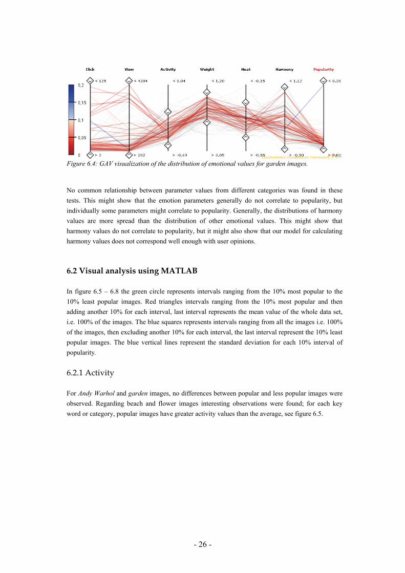
6.1.4 Garden Popular garden images tend to have low activity values, high weight values and low heat values, i.e popular garden images tend to be experienced passive, heavy and cold. This might suggest that these three emotional values are correlated to popularity. The distributions of harmony values are spread, this might show that harmony do not correlate to popularity, see figure 6.4.

- 26 -

Figure 6.4: GAV visualization of the distribution of emotional values for garden images.

No common relationship between parameter values from different categories was found in these tests. This might show that the emotion parameters generally do not correlate to popularity, but individually some parameters might correlate to popularity. Generally, the distributions of harmony values are more spread than the distribution of other emotional values. This might show that harmony values do not correlate to popularity, but it might also show that our model for calculating harmony values does not correspond well enough with user opinions.

6.2 Visual analysis using MATLAB

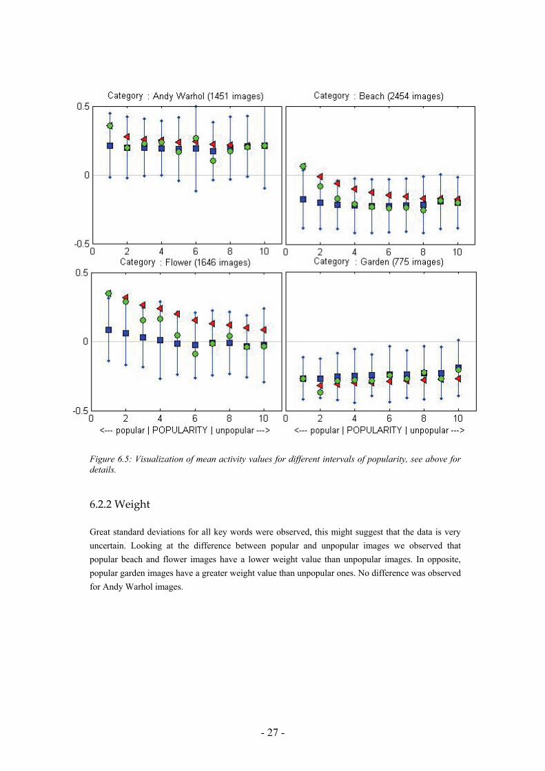
In figure 6.5 – 6.8 the green circle represents intervals ranging from the 10% most popular to the 10% least popular images. Red triangles intervals ranging from the 10% most popular and then adding another 10% for each interval, last interval represents the mean value of the whole data set, i.e. 100% of the images. The blue squares represents intervals ranging from all the images i.e. 100% of the images, then excluding another 10% for each interval, the last interval represent the 10% least popular images. The blue vertical lines represent the standard deviation for each 10% interval of popularity.

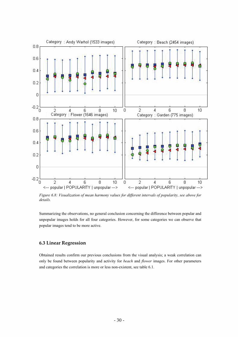
6.2.1 Activity

For Andy Warhol and garden images, no differences between popular and less popular images were observed. Regarding beach and flower images interesting observations were found; for each key word or category, popular images have greater activity values than the average, see figure 6.5.

- 27 -

Figure 6.5: Visualization of mean activity values for different intervals of popularity, see above for details.

6.2.2 Weight

Great standard deviations for all key words were observed, this might suggest that the data is very uncertain. Looking at the difference between popular and unpopular images we observed that popular beach and flower images have a lower weight value than unpopular images. In opposite, popular garden images have a greater weight value than unpopular ones. No difference was observed for Andy Warhol images.

- 28 -

Figure 6.6: Visualization of mean weight values for different intervals of popularity, see above for details. .

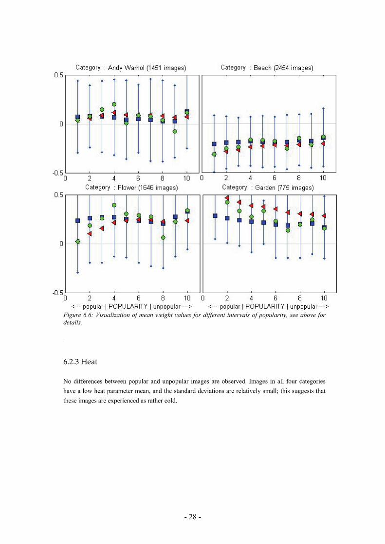
6.2.3 Heat

No differences between popular and unpopular images are observed. Images in all four categories have a low heat parameter mean, and the standard deviations are relatively small; this suggests that these images are experienced as rather cold.

- 29 -

Figure 6.7: Visualization of mean heat values for different intervals of popularity, see above for details. Notify the different scale on the upper left plot.

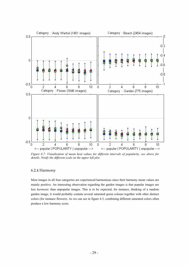
6.2.4 Harmony

Most images in all four categories are experienced harmonious since their harmony mean values are mainly positive. An interesting observation regarding the garden images is that popular images are less harmonic than unpopular images. This is to be expected, for instance, thinking of a random garden image, it would probably contain several saturated green colours together with other distinct colors (for instance flowers). As we can see in figure 4.3, combining different saturated colors often produce a low harmony score.

- 30 -

Figure 6.8: Visualization of mean harmony values for different intervals of popularity, see above for details. Summarizing the observations, no general conclusion concerning the difference between popular and unpopular images holds for all four categories. However, for some categories we can observe that popular images tend to be more active.

6.3 Linear Regression

Obtained results confirm our previous conclusions from the visual analysis; a weak correlation can only be found between popularity and activity for beach and flower images. For other parameters and categories the correlation is more or less non-existent, see table 6.1.

- 31 -

Activity Weight Heat Harmony Average Andy Warhol 0,081 -0,0093 0,0464 -0,0341 0,021 Beach 0,2112 -0,0611 -0,0906 -0,0234 0,009025 Flower 0,2041 -0,0938 0,0179 0,0297 0,039475 Garden -0,0138 0,1384 0,0814 -0,104 0,0255 Average 0,120625 -0,00645 0,013775 -0,03295

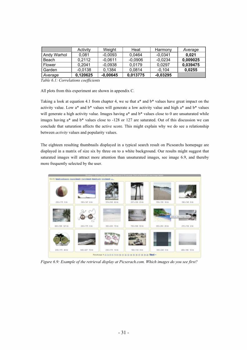
Table 6.1: Correlations coefficients All plots from this experiment are shown in appendix C. Taking a look at equation 4.1 from chapter 4, we se that a* and b* values have great impact on the activity value. Low a* and b* values will generate a low activity value and high a* and b* values will generate a high activity value. Images having a* and b* values close to 0 are unsaturated while images having a* and b* values close to -128 or 127 are saturated. Out of this discussion we can conclude that saturation affects the active score. This might explain why we do see a relationship between activity values and popularity values. The eighteen resulting thumbnails displayed in a typical search result on Picsearchs homepage are displayed in a matrix of size six by three on to a white background. Our results might suggest that saturated images will attract more attention than unsaturated images, see image 6.9, and thereby more frequently selected by the user.

Figure 6.9: Example of the retrieval display at Picserach.com. Which images do you see first?

- 32 -

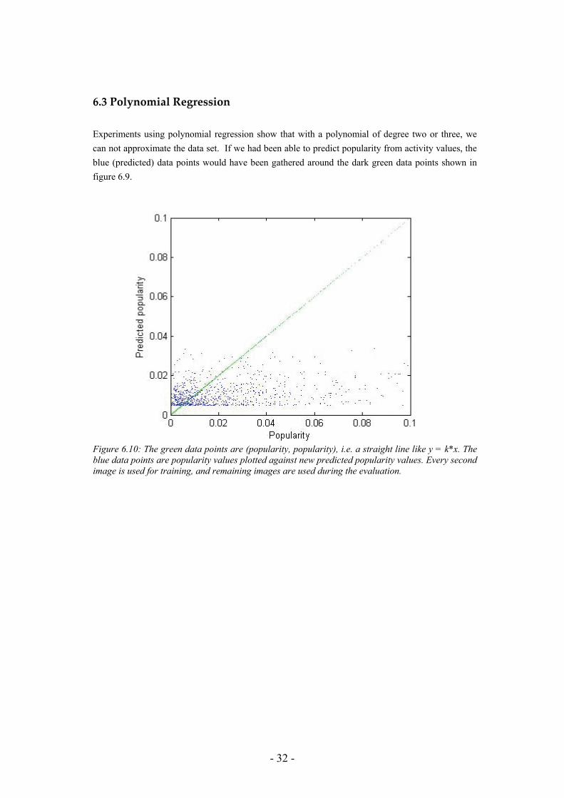
6.3 Polynomial Regression Experiments using polynomial regression show that with a polynomial of degree two or three, we can not approximate the data set. If we had been able to predict popularity from activity values, the blue (predicted) data points would have been gathered around the dark green data points shown in figure 6.9.

Figure 6.10: The green data points are (popularity, popularity), i.e. a straight line like y = k*x. The blue data points are popularity values plotted against new predicted popularity values. Every second image is used for training, and remaining images are used during the evaluation.

- 33 -

Chapter 7

Discussion and Future Work Even though the results weren’t what we had been hoping for, still they are meaningful. We have shown that it exist relations between emotional values from specific keywords and our definition of popularity. However, no common relation between the emotional values and popularity for all keywords was found. Our method was designed as a pilot study and several improvements can be taken into consideration for further investigations.

7.1 Discussion

We proposed the ratio between gathered click and views as a value of user popularity. These values are just approximations of a more complex reality, which we at the moment might only theoretically analyze. It is questionable whether a quotient between click and view is an appropriate measurement since there is a great difference between the numbers of views for the images. For instance, if an image have been viewed a hundred thousand times and been clicked ten thousand times, is this image less popular than an image being viewed fifty times and clicked twelve times? Problems caused by this difference in scale will be even more obvious since most images in the database have popularity values less than 0,050. Consequently, the difference between popular images and unpopular images is very fine. For instance, an image being viewed fifty times getting just another click might be directly regrouped from the 10% least popular to the 10% most popular images (in the previous experiments), which might produce unreliable data. At this point we do not exactly know what content that affects an average user when judging a random displayed image. For instance, we do not know to which extent color actually affect users in their decisions. The object itself as well as the image quality might have an even greater impact on decisions. We can neither be sure that an image that has been displayed and not clicked actually have been seen or judged by the user. The color emotion values predicted from the models derived by Li Chen et. al are developed using perfect color samples viewed under very controlled conditions. During the development phase, test users are not affected by any other surrounding colors, shapes or objects attracting their focus. It is not without any doubts we apply the model on color images. Due to the approximation, the colors from histograms we use as input to the predictive models might not be those the users see in the images. The color harmony model was proposed for color pairs positioned beside each other. When choosing the most represented colors from the histograms, it is not certain that the colors are positioned beside each other in the image. For some images we can not reject that colors in the middle and colors of distinct objects can have a greater impact on the overall color experience than colors in the outer edge.

- 34 -

To test and verify whether these implementations of the predictive models correspond well with user opinions, further empirical investigations needs to be done. Such studies and verification experiments are previously ongoing at ITN.

7.2 Future Work We have concluded that the user data in combination with our approximation of measuring popularity might be uncertain. More information about the way user makes their choices is desirable. For instance, the order which the user click the images are of interest. The probability that a user click an image on the first display is probably greater than on the fifth, therefore, the number of the page is of great interest. A large set of images are needed for an analysis like this. A tradeoff between time efficiency and certainty of data is obvious, but the gatherings do not need to be done from the public search interface. It can be done in a different and more reliable way, for instance using groups of test users that are given single tasks. The tasks can for instance be to choose between two images A and B. The advantage is less effort while the disadvantage is that the result only gives us order between images, not the distance. Another disadvantage is that it demands many appraisals. We can also ask test users to rank the order of a set of images, the benefit is that the answers are easier to evaluate. Asking users to place images on a scale and register absolute positions gives us the possibility to evaluate differences in distances. However, with most user tests, a disadvantage occurs during the first appraisals when users have no references to compare with.

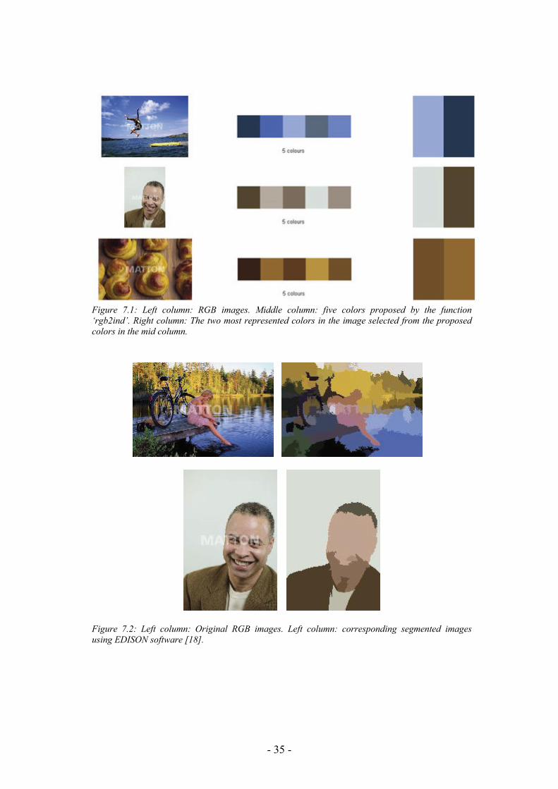
Instead of using color histograms, we propose to use MATLAB’s own color index function, rgb2ind for choosing input colors. The function converts an RGB image to an indexed image, reducing the numbers of colors. Correct configured, the function find the colors in the specified colormap that best match the colors in the RGB image, see figure 7.1.

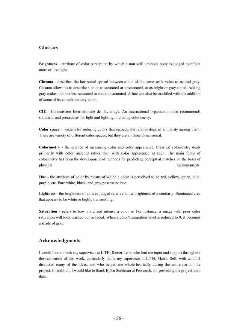
Using image segmentation we can also retrieve positions of solid color fields in the image, consequently we can consider if the colors are neighbours or not when calculating harmony values. We can also consider whether the color fields belong to an object or not, i.e. if the color might attract the users attention more or less, when calculating the emotional values. Examples of image segmentation using EDISON software [26] are shown in figure 7.2. In this thesis we have only taking the color content of an image into consideration. Other low level features, for instance quality of the image, focal depth or sharpness might affect the selection of an image. Since the popularity values are not normally distributed, as discussed in previous section, a strategy worth trying would be transforming the popularity data prior to finding correlations. For instance, performing square root transformations or logarithmic transformations on the data set can possibly lead to a better correlation.

- 35 -

Figure 7.1: Left column: RGB images. Middle column: five colors proposed by the function ‘rgb2ind’. Right column: The two most represented colors in the image selected from the proposed colors in the mid column.

Figure 7.2: Left column: Original RGB images. Left column: corresponding segmented images using EDISON software [18].

- 36 -

Glossary

Brightness - attribute of color perception by which a non-self-luminous body is judged to reflect more or less light. Chroma - describes the horizontal spread between a hue of the same scale value as neutral gray. Chroma allows us to describe a color as saturated or unsaturated, or as bright or gray-tinted. Adding gray makes the hue less saturated or more unsaturated. A hue can also be modified with the addition of some of its complementary color. CIE - Commission Internationale de l'Eclairage. An international organization that recommends standards and procedures for light and lighting, including colorimetry. Color space - system for ordering colors that respects the relationships of similarity among them. There are variety of different color spaces, but they are all three dimensional. Colorimetry - the science of measuring color and color appearance. Classical colorimetry deals primarily with color matches rather than with color appearance as such. The main focus of colorimetry has been the development of methods for predicting perceptual matches on the basis of physical measurements. Hue - the attribute of color by means of which a color is perceived to be red, yellow, green, blue, purple, etc. Pure white, black, and grey possess no hue. Lightness - the brightness of an area judged relative to the brightness of a similarly illuminated area that appears to be white or highly transmitting. Saturation - refers to how vivid and intense a color is. For instance, a image with poor color saturation will look washed out or faded. When a color's saturation level is reduced to 0, it becomes a shade of gray.

Acknowledgments

I would like to thank my supervisor at LiTH, Reiner Lenz, who lent me input and support throughout the realization of this work, particularly thank my supervisor at LiTH, Martin Solli with whom I discussed many of the ideas, and who helped me whole-heartedly during the entire part of the project. In addition, I would like to thank Björn Sundman at Picsearch, for providing the project with data.

- 37 -

Bibliography

[1] Gaurav Sharma, Digital Color Imaging Handbook, Xerox Corporation Webster, New York (2003). [2] Mark D. Fairchild, Color Appearances Models, First Edition, Addison-Wesley, Massachusetts (1998). [4] E.J. Giorgianni and T.E. Madden, Digital Color Management, Encoding Solutions, Addison-Wesley, Massachusetts (1998). [5] Xiao-Ping Gao, Joh H. Xin, Investigation of Human’s Emotional Response on Colors, The Hong Kong Polytechnic University, Hong Kong (2006). [6] Peter K. Kaiser & Robert M. Boynton, Human Color Vision, Second Edition, Optical Society of America, Washington (1996) [7] Tran L.V. Efficient Image Retreival with Statistical Color Descriptors, Linköping University, Campus Norrköping, Norrköping (2003). [8] L. Johansson Human Color Vision, Linköping University, Campus Norrköping, Norrköping (2004) [9] Th. Gevers and A.W.M Smeulders, Image Search Engines – An Overview, University of Amsterdam, Faculty of Science, Amsterdam, (2004) [10] M. Stricker and M. Orengo, Similarity of Color Images, Swiss Federal Institute of Technology, ETH, Zurich, (1996) [11] Jia Wang, Wen-jam Yang and Raj Acharya, Color Clustering Techniques for Color-Content-Based Image Retrieval from Image Databases, Department of Electrical and Computer Engineering, State University of New York at Buffalo, Buffalo (1997). [12] N. Jacobson and W.Bender, Color as a determined communication, IBM Systems, (1996). [13] Gao, Xin, Sato et.al, Analysis of Cross-Cultural Colour Emotion, Various Universities (2006). [14] Li-Chen Ou et.al, A Study of Color Emotion and Colour Preferences, Part I: Colour Emotions for Singel Colours, University of Derby, Kingsway, Derby (2004). [15] Li-Chen Ou et.al, A Study of Color Emotion and Color Preferences, Part II: Colour Emotions for Two Colour Combinations, University of Derby, Kingsway, Derby (2004).

- 38 -

[16] Li-Chen Ou et.al, A Study of Color Emotion and Color Preferences, Part III: Colour preference modelling, University of Derby, Kingsway, Derby (2004). [17] Li-Chen Ou, M. Ronnier Lou, A Colour Harmony Model for Two-Colour Combinations, University of Leeds, Leeds LS2 9JT, United Kingdom (2006). [18] Martin Solli and Reiner Lenz, Color Emotions for Image Classification and Retrieval, in Proceedings of 'CGIV 2008', Barcelona, Spain (2008). [19] Cambridge In Color, http://www.cambridgeincolour.com. [20] Richard B. Darlington, Factor Analysis, retrieved 22:nd of April 2008 from http://www.psych.cornell.edu/darlington/ [21] VITA Institution at Linköping University, Campus Norrköping, retrieved 22:nd of April 2008 from http://vita.itn.liu.se/gav/ [22] Svante Körner and Lars Wahlgren, Praktisk statistik, Statistical Insitution of Lund University, Studentlitteratur (2002). [23] Gurura H, MacDonald LW, Dalke H, Background: an essential factor in color harmony. In: Proceedings of the Interim Meeting of International Color Association, AIC (2004). [24] Larry D Schroeder et.al, Understanding Regression Analysis: An Introductory Guide, Newbury Park, CA, (1986). [25] John McDonald, Online Handbook of Biological Statistics, retrieved 25:th of April 2008 from http://udel.edu/~mcdonald/statintro.html [26] The D. Comanicu, P. Meer: Mean shift: A robust approach toward feature space analysis. IEEE Trans. Pattern Anal. Machine Intell., 24, 603-619, May 2002. Software retrieved December 14:th from http://www.caip.rutgers.edu/riul/research/code/EDISON/index.html [27] M. Sokes, M Andersson, A Standard Default Color Space for the Internet – sRGB, retrieved May 15:th from http://www.w3.org/Graphics/Color/sRGB.html

- 39 -

Appendix A

Color Science What is color? Some would say colors are attributes describing objects while others would say that color is something that is generated in our mind and brain. Giving the word color a good definition provides some interesting challenges and difficulties. Many scientists have put great efforts to attempt describing the nature of light and color, both in a physical and a psychological meaning. Color can briefly be described as an interaction of three elements; an illuminant, an object and an observer [1]. Without an illuminant (light source), nothing could be seen. We do see objects around us, but in fact it is not the objects themselves that we see, the correct thing to say is that we see reflected, transmitted through or emitted light from the objects. Color also has to be observed to get a human meaning, or as Mark D. Fairchild wrote: “It is often asked whether a tree falling in the forest makes a sound if no one is there to observe it. Perhaps equal philosophical energy should be spent wondering what color its leaves are if no one is there to see them” [2]. The following sections will briefly describe the fundamentals of color science.

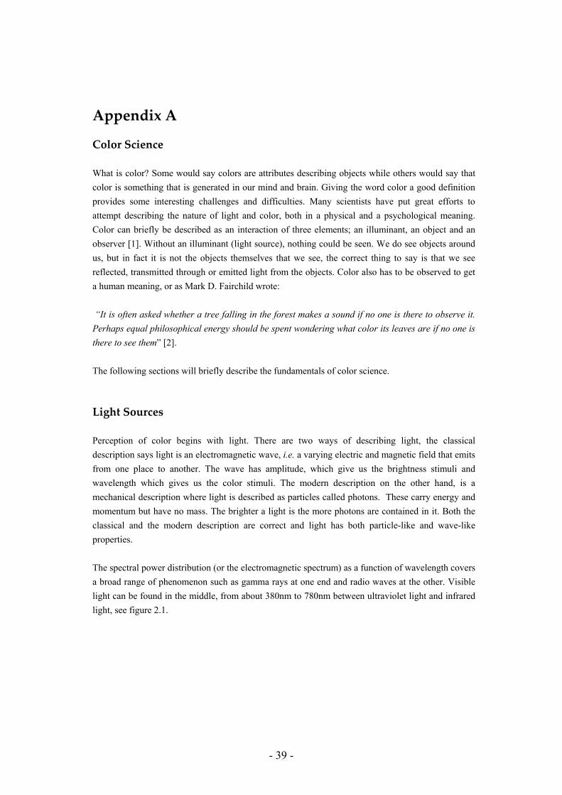
Light Sources Perception of color begins with light. There are two ways of describing light, the classical description says light is an electromagnetic wave, i.e. a varying electric and magnetic field that emits from one place to another. The wave has amplitude, which give us the brightness stimuli and wavelength which gives us the color stimuli. The modern description on the other hand, is a mechanical description where light is described as particles called photons. These carry energy and momentum but have no mass. The brighter a light is the more photons are contained in it. Both the classical and the modern description are correct and light has both particle-like and wave-like properties. The spectral power distribution (or the electromagnetic spectrum) as a function of wavelength covers a broad range of phenomenon such as gamma rays at one end and radio waves at the other. Visible light can be found in the middle, from about 380nm to 780nm between ultraviolet light and infrared light, see figure 2.1.

- 40 -

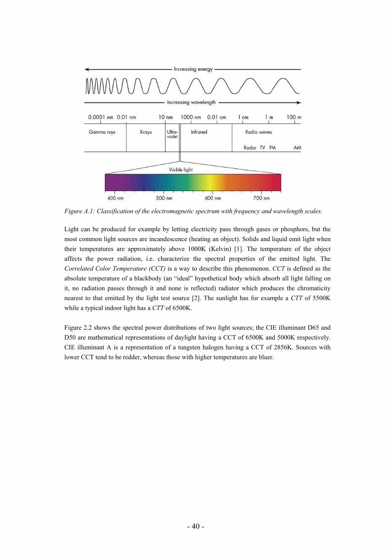
Figure A.1: Classification of the electromagnetic spectrum with frequency and wavelength scales. Light can be produced for example by letting electricity pass through gases or phosphors, but the most common light sources are incandescence (heating an object). Solids and liquid emit light when their temperatures are approximately above 1000K (Kelvin) [1]. The temperature of the object affects the power radiation, i.e. characterize the spectral properties of the emitted light. The Correlated Color Temperature (CCT) is a way to describe this phenomenon. CCT is defined as the absolute temperature of a blackbody (an “ideal” hypothetical body which absorb all light falling on it, no radiation passes through it and none is reflected) radiator which produces the chromaticity nearest to that emitted by the light test source [2]. The sunlight has for example a CTT of 5500K while a typical indoor light has a CTT of 6500K. Figure 2.2 shows the spectral power distributions of two light sources; the CIE illuminant D65 and D50 are mathematical representations of daylight having a CCT of 6500K and 5000K respectively. CIE illuminant A is a representation of a tungsten halogen having a CCT of 2856K. Sources with lower CCT tend to be redder, whereas those with higher temperatures are bluer.

- 41 -

Figure A.2: The relative spectral power distribution for the, CIE illuminant D50 (dot line), CIE illuminant D65 (solid line) and the CIE illuminant A (dashdot line).

Objects When light hits an object it can be reflected, absorbed, scattered, refracted or/and transmitted. The effect depends both on the physical characteristics of the surface and the substance of the object itself. If the surface of the object is glossy, i.e. has a smooth surface, the light is reflected as a mirror in the same angle as the incoming light according to the surface normal. All light beams are not reflected (unless the object is a perfect mirror), some beams are absorbed by the object and are converted to heat. The amount of absorbed light depends on the transparency of the object, the less transparency the more light will be absorbed. Some light beams are neither reflected nor absorbed, instead they are refracted, i.e. change direction when it passes trough a medium and finally transmitted trough the object.

Color Stimuli The “colors” we see or measure, are in color science terminology called color stimulus. These stimulus are in fact light, light that has been reflected from or reflected through an object (in some cases the light comes directly from the source it self). A color stimulus is, in a facilitated case, represented as a function of wavelength and is defined as the product of the power of the light source and the reflectance of the object at each wavelength [4]. Consequently the color stimulus will change when changing the light. How a stimulus appears does not only depend on the spectral properties, it also depends on many other factors such as size, shape,

- 42 -

spatial properties to name a few. These are beyond the limits of this report and the interested reader is referred to [2].

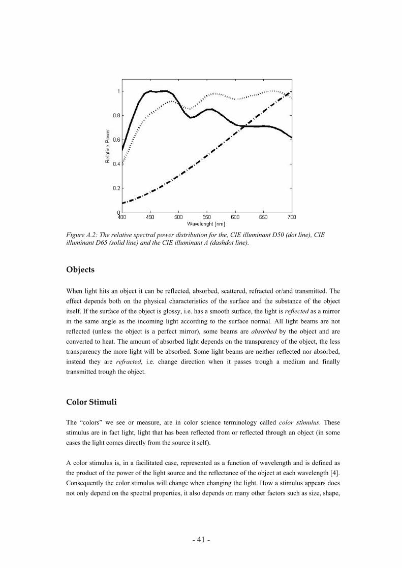
Human Color Vision The incident light is focused and refracted by the cornea and the eyes lens, se figure 2.6. This will make a projection of the light onto the retina located in the back of the eyeball. To analyze the incident light the retina consists of two types of photoreceptors, rods and cones. The rods are basically monochromatic and extremely sensitive to light, therefore do they not contribute to color vision, and instead they are very useful in dark conditions. During the night we can see shapes and movements, but hardly any colors. The other sensor type, the cones, gives us the color sensation. There are three different types of cones, L, M and S cones having maximal sensitivity at 575nm, 535nm and 445nm respectively, in other words they are sensitive to light in different wavelengths. Under a fixed set of viewing conditions, the response of these cones can be approximated by [1]:

∫=max

min

)()(λ

λ

λλλ dfsC ii i = 1,2,3… (2.3)

The eye contains a lot more L and M cones than S cones, the relative population is 40:20:1. Therefore the brain needs to compare and weight the signal from the different cones and its neighbors. This process allows the human visual system to distinguish very small differences in stimulation of the three types of photoreceptors. It has been established that they can give rise to about ten million distinguishable color sensations.

Figure A.3: Schematic of the human eye Because of this trichromatic nature of human vision it is possible that two different spectral distributions will give rise to identical color stimuli. This phenomenon, called metamerism, is an advantage when reproducing color in different color-applications, since it’s only necessary to produce a stimulus that is visual equivalent to the original. Metamerism can also be a disadvantage; two equal experienced colors viewed under light source A can look completely different when viewed under light source B.

- 43 -

Appendix B

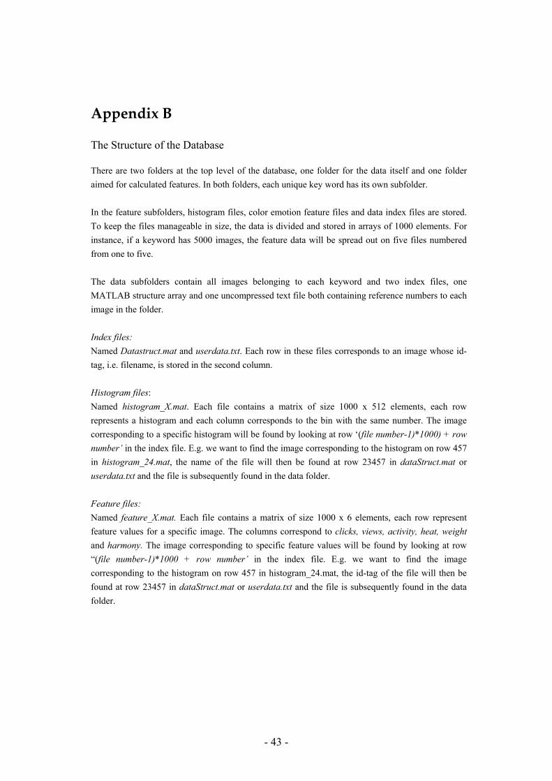
The Structure of the Database

There are two folders at the top level of the database, one folder for the data itself and one folder aimed for calculated features. In both folders, each unique key word has its own subfolder. In the feature subfolders, histogram files, color emotion feature files and data index files are stored. To keep the files manageable in size, the data is divided and stored in arrays of 1000 elements. For instance, if a keyword has 5000 images, the feature data will be spread out on five files numbered from one to five. The data subfolders contain all images belonging to each keyword and two index files, one MATLAB structure array and one uncompressed text file both containing reference numbers to each image in the folder. Index files: Named Datastruct.mat and userdata.txt. Each row in these files corresponds to an image whose id-tag, i.e. filename, is stored in the second column.

Histogram files: Named histogram_X.mat. Each file contains a matrix of size 1000 x 512 elements, each row represents a histogram and each column corresponds to the bin with the same number. The image corresponding to a specific histogram will be found by looking at row ‘(file number-1)*1000) + row number’ in the index file. E.g. we want to find the image corresponding to the histogram on row 457 in histogram_24.mat, the name of the file will then be found at row 23457 in dataStruct.mat or userdata.txt and the file is subsequently found in the data folder. Feature files: Named feature_X.mat. Each file contains a matrix of size 1000 x 6 elements, each row represent feature values for a specific image. The columns correspond to clicks, views, activity, heat, weight and harmony. The image corresponding to specific feature values will be found by looking at row “(file number-1)*1000 + row number’ in the index file. E.g. we want to find the image corresponding to the histogram on row 457 in histogram_24.mat, the id-tag of the file will then be found at row 23457 in dataStruct.mat or userdata.txt and the file is subsequently found in the data folder.

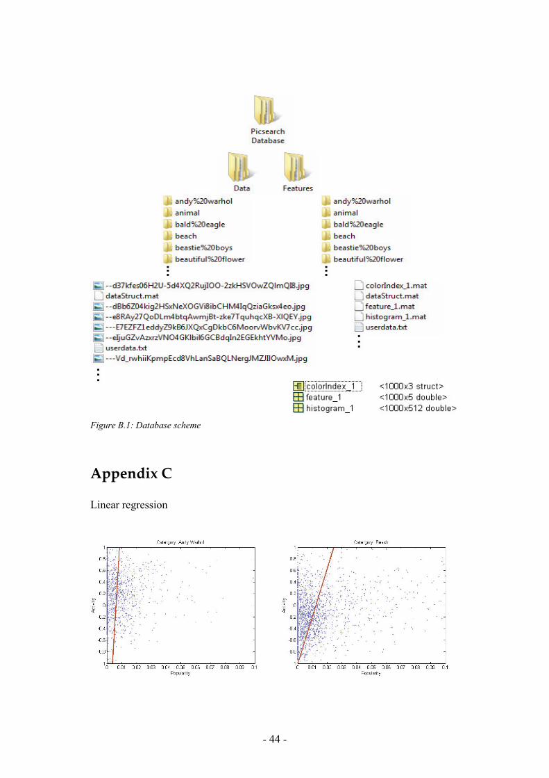
- 44 -

Figure B.1: Database scheme

Appendix C

Linear regression

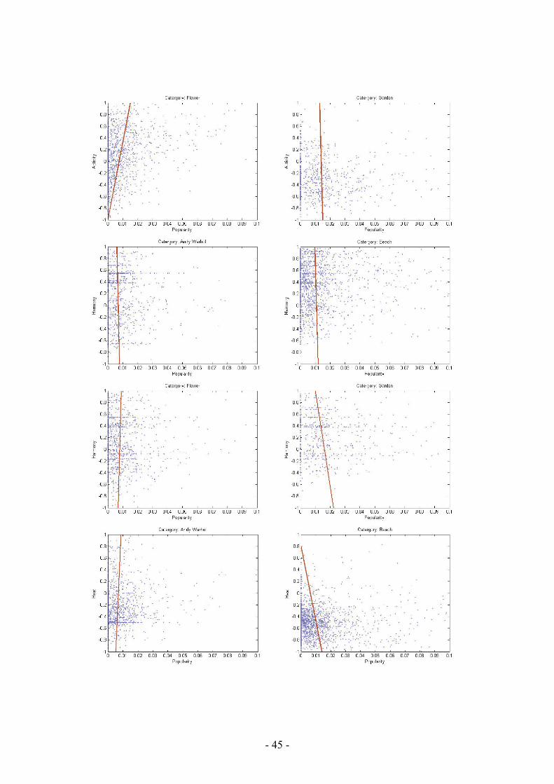
- 45 -

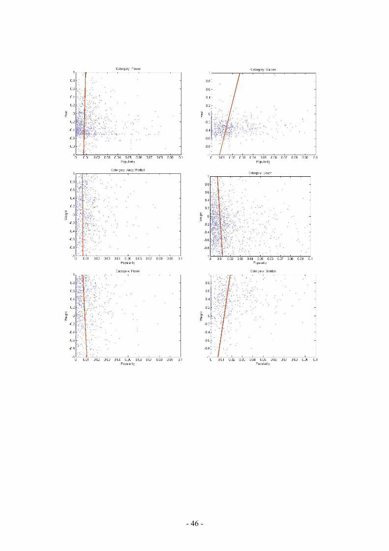
- 46 -