relationship between trade liberalisation, growth and...

Relationship betweenTrade Liberalisation,Growth and Balance ofPayments in DevelopingCountries:An EconometricStudy

Ashok Parikh

HWWA DISCUSSION PAPER

286Hamburgisches Welt-Wirtschafts-Archiv (HWWA)

Hamburg Institute of International Economics2004

ISSN 1616-4814

Hamburgisches Welt-Wirtschafts-Archiv (HWWA)Hamburg Institute of International EconomicsNeuer Jungfernstieg 21 – 20347 Hamburg, GermanyTelefon: 040/428 34 355Telefax: 040/428 34 451e-mail: [email protected]: http://www.hwwa.de

The HWWA is a member of:

• Wissenschaftsgemeinschaft Gottfried Wilhelm Leibniz (WGL)• Arbeitsgemeinschaft deutscher wirtschaftswissenschaftlicher Forschungsinstitute

(ARGE)• Association d’Instituts Européens de Conjoncture Economique (AIECE)

mailto:[email protected]

http://www.hwwa.de/

HWWA Discussion Paper

Relationship between TradeLiberalisation, Growth and

Balance of Payments in DevelopingCountries:

An Econometric Study

Ashok Parikh

HWWA Discussion Paper 286http://www.hwwa.de

Hamburg Institute of International Economics (HWWA)Neuer Jungfernstieg 21 – 20347 Hamburg, Germany

e-mail: [email protected]

This paper was prepared while the author was visiting the Hamburg Institute ofInternational Economics, Hamburg, Germany. The author wishes to thank Dr. CarstenHefeker and participants at the seminar for their useful comments and the LeverhulmeTrust for the Emeritus award.

Edited by the Department World EconomyHead: PD Dr. Carsten Hefeker

HWWA DISCUSSION PAPER 286July 2004

Relationship between TradeLiberalisation, Growth and Balance

of Payments in DevelopingCountries:An Econometric Study

ABSTRACT

The objectives of this paper are to study the impact of liberalisation on trade deficits andcurrent accounts of developing countries. It is expected that trade liberalisation wouldpromote economic growth from the supply side by leading to a more efficient use ofresources, by encouraging competition, and by increasing the flow of ideas andknowledge across national boundaries. Trade liberalisation could lead to faster importgrowth than export growth and hence the supply side benefits may be offset by theunsustainable balance of payments position. This study uses panel data of 42 countries(both time-series and cross-section dimension) to estimate the effect of tradeliberalisation and growth on trade balance while controlling for other factors such asincome terms of trade. The major finding of the study is that trade liberalisationpromotes growth in most cases, (Part 1 of this study) the growth itself has a negativeimpact on trade balance and this in turn could have negative impacts on growth throughdeterioration in trade balance and adverse terms of trade. Our conclusion is that tradeliberalisation could constrain growth through adverse impact on balance of payments.

Key Words: Panel data, Income Terms of Trade, Dynamic Optimisation, Dynamicpanel model

JEL-Classification: C21, C22, C23, F13, F14, F32

Ashok ParikhSchool of Economics and Social StudiesUniversity of East Anglia, NorwichNR4 7TJ, United KingdomPhone: +44-1603-592714Fax: +44-1603-250434e-mail: A.Parikh@uea-ac-uk

mailto:A.Parikh@uea-ac-uk

1

Introduction

This study extends the previous work (Parikh and Stirbu, 2004) where static models have

been used to study the relationship between trade liberalisation and economic growth and

the joint impact of liberalisation and growth on trade balance. Our previous models and

analysis can be useful to draw certain inferences but otherwise, it was analytically less

strong as there existed problems of serial correlation with econometric estimation on

panel or time series data. Moreover, specification of trade balance relationship did not

consider a multivariate dynamic specification based on optimisation theory in

international economics. However, the study highlighted some major sets of variables

which can be considered in a dynamic setting. The objectives of this study are to examine

the impact of liberalisation, growth and trade policy variables on the trade balance and

current account balances in a panel framework for developing countries where the data

are for each country over time and these countries are all treated together. We also

estimate dynamic models on panel data.

We first define the current account in a more appropriate manner than just the residual

from the balance of exports of goods and services less imports of goods and services. A

current account deficit can be defined as the country’s excess of investment over savings.

However, the saving and investment flows reported in many national income accounts do

not conform closely to the theoretically correct concepts of saving and investment when

international capital mobility is extensive. Historically, current account balances were

small in post-1945 period. Initially this was because of official restrictions on

international capital movements as most industrialised countries’ currencies were

inconvertible until 1959. After the early 1970s net international capital flows have

expanded as a result of petrodollar recycling, the removal of many industrial country

restrictions on international payments following the adoption of floating exchange rates

and the technological evolution in the financial industry. This means that we have to

consider definition of current account which is sensitive to capital inflows and outflows

including service payments.

2

In section 2 of the paper we provide comparison of the decade 1990s with 1980s in terms

of trade balance and economic growth in developing countries and regions of these

developing countries. In section 3 we provide a model to link trade balance or current

account with the domestic growth. This is based on the consumption smoothing principle

for the nation and follows dynamic optimisation under current account constraint. In

section 4, the corresponding dynamic model is estimated using dynamic panel data

technique. We first allow for the endogenity of growth variable in such a procedure and

then we permit other variables to be treated endogenously with growth. In section 5, we

attempt regional analysis for two regions namely Africa and Latin America (including

Asian countries) and present some of the contrasting features of the results. Since we

have only small number of Asian countries in our sample, a separate analysis was not

conducted although they form a part of the 42 countries and also of Latin American

region. In section 6, we draw some conclusions of the study.

2 Non-fuel exporting developing countries excluding China

We consider the period 1980-1989 decade and compare it with 1990-1999 decade as far

as trade balance and current account deficits are concerned for developing countries.

There was a strong improvement in external balance of developing countries. While the

improvement in the external accounts during the crisis and adjustment period of the early-

1980s were associated mainly with import compression and falling growth, the

relationship between external account and growth became virtuous and very unusual for

the short period between 1983 and 1985 when external accounts improved with rising

growth. Then, there was a strong deterioration in the external position between the years

1987–88 and the mid-1990s with a swing back to a deficit level similar to that of the

previous decade. Two features of the post-1987 period stand out. (i) The period 1987–90

was characterized by increasing external deficits and slowing growth, i.e. a constellation,

which is clearly unsustainable in the long run. During this period many developing

countries also underwent a regime change in their trade policy in the sense that they

dismantled quantitative restrictions and reduced tariffs, and that they maintained this

stance in spite of a worsening trade account. In other words, they stopped using trade

3

policy measures for balance-of-payments purposes. (ii) Even though economic growth in

developing countries picked up moderately after 1990, the rates achieved are associated

with higher external deficits (to GDP ratios) than in previous periods. This means that

over the past decade there has been an increase in the external financing requirement

associated with any given growth rate. As a matter of fact, the relationship between

growth and the external position of the past few years mimics that of the period prior to

the economic crisis of the early-1980s.

The evolution of the current account position in the non-fuel-exporting-developing

countries excluding China has been largely determined by the evolution of their trade and

income accounts, while their balances on services and current transfers have not been

subject to important changes over the past three decades.1 The decline in world interest

rates since 1989 has reduced the pressure of debt service payments on the current account

but this has not translated into lower current-account deficits due to the renewed

deterioration in the trade account. Between the 1980s and the 1990s, trade deficits of

developing countries increased strongly with the rate of growth remaining by and large

unchanged. There are a few notable exceptions from this basic pattern of a similar

deficit/GDP ratio and a lower growth rate in the 1990s compared with the decade prior to

1980s:

— the average external trade position of developing countries including the major

fuel-exporting countries has worsened throughout the period;

— the group of non-fuel exporting countries in sub-Saharan Africa has experienced

a worsening of both its external position and its growth rate;

— the group of non-fuel developing Asia excluding China raised its growth rate

while improving its external position during the 1980s; it is the only region for

which the relationship in the first half of the 1990s is not substantially different

from that in the 1970s.

1 The GDP-ratio of the services account has fluctuated between 0 and –0.5 per cent, while that of the

current transfers has fluctuated between 1.5 and 2.0 per cent. With the fuel-exporting developingcountries included, the average services/GDP ratio becomes –0.8 to –3.0 per cent and that of the currenttransfer/GDP ratio 0 to 0.8 per cent. For detailed empirical evidence, see Table A31 in InternationalMonetary Fund, World Economic Outlook, various issues.

4

Statistical evidence shows that after a continuous increase of both exports and imports of

developing countries during the 1970s, their exports stagnated and their imports dropped

during the first half of the 1980s. By contrast, both imports and exports have risen

strongly since 1986. Looking at regional sub-groups suggests that the drastic

improvement in the trade balance of non-fuel developing America during the 1980s were

due to a slight increase in exports but mainly due to a very substantial compression of

imports. This contrasts sharply with the experience of non-fuel developing Asia

excluding China whose trade balance improved in the 1980s due mainly to a very strong

increase in exports-contrary to developing America, imports also increased. Hence, while

import compression is likely to have choked economic growth in developing America,

rising imports were associated with rising growth and rising exports in developing Asia.

Sub-Saharan Africa is the other developing region that experienced strong import

compression during the 1980s and, contrary to the situation in developing America, this

experience has not very much improved over the past few years.

Individual country experience

The external trade position deteriorated in the majority of countries, while the majority of

countries experienced rising growth rates between the 1980s and the 1990s. However, 15

out of the 29 countries with a deteriorating external trade position and rising growth

between the 1980s and the 1990s are in developing America (Table 1). It is also

noteworthy that, between the 1980s and the 1990s, all the developing countries, which

have been affected most by the recent financial crisis, (i.e. Brazil, Indonesia, Korea,

Malaysia and Thailand) experienced a worsening in their external trade position and thus

an increase in their external financing requirements.

A perhaps somewhat surprising feature is that Singapore is the only main exporter of

manufactures whose external trade position has improved between the 1980s and the

1990s, while that of Hong Kong, Korea, Malaysia, Mexico, Taiwan, Thailand and Turkey

has worsened. It should not be forgotten, however, that exports with a comparatively

high-income elasticity of demand encompasses a much broader spectrum than

manufactures. Some countries in the sample have been able to increase exports of agro-

industrial goods, such as for example Chile, where export earnings from fruit and fishery

5

and forestry products have, together, come to rival those from copper, and this has helped

her to achieve both increased growth and an improved external position between the

1970s and the 1990s.

3 Theoretical base of current account and GDP growth relationship

In this section we propose a dynamic model to study the relationship between GDP

growth and trade balance to GDP ratios. This theoretical model is largely for developed

countries but it provides the framework for the relationship between trade balance and

GDP growth rates when debt-GDP ratio is constant.

We consider a small open economy inhabited by a representative agent with an infinite

time horizon. The economy starts in period t and continues forever. We normalize

population size to unity. The utility function for infinite period is

)U(CβU(t) sts

ts∑∝

=

−= (3.1)

where Cs is consumption in period s and β is the discount rate. Deriving the t period-

budget constraint, the current account with constant interest rate is

CAt = Bt+1 –Bt = Yt + rBt –C t – G t - I t (3.2)

where CA is current account, B is net foreign assets accumulated on prior dates, I is

investment and is equivalent to changes in capital stock, C is consumption, G is

government expenditure, t refers to the time period.

There is an accounting equivalence between the net export surplus in current account and

the negative value of the capital account. The current account balance as defined in

equation (3.2) is the changes in net foreign assets position between two periods.

If output is determined by Y= AF(K) i.e. output is a function of capital K (accumulated

over previous periods) with A as the given technology, the utility function after

substitution for consumption in period s will be

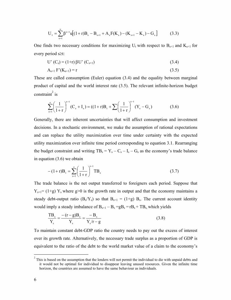
6

[ ]ss1sss1ssts

tst G)K(K)F(KABr)B(1uβU −−−+−+= ++

∝

=

−∑ (3.3)

One finds two necessary conditions for maximizing Ut with respect to Bs+1 and Ks+1 for

every period s≥t:

U’ (Cs) = (1+r) βU’ (Cs+1) (3.4)

As+1 F’(Ks+1) = r (3.5)

These are called consumption (Euler) equation (3.4) and the equality between marginal

product of capital and the world interest rate (3.5). The relevant infinite-horizon budget

constraint2 is

)G(Yr1

1r)B((1)I(Cr1

1ss

ts

tss

ts

ts

−

+

++=+

+

−−∝

=∑∑ (3.6)

Generally, there are inherent uncertainties that will affect consumption and investment

decisions. In a stochastic environment, we make the assumption of rational expectations

and can replace the utility maximization over time under certainty with the expected

utility maximization over infinite time period corresponding to equation 3.1. Rearranging

the budget constraint and writing TBs = Ys – Cs – Is – Gs as the economy’s trade balance

in equation (3.6) we obtain

s

ts

tst TB

r11r)B(1

−∝

=∑

+

=+− (3.7)

The trade balance is the net output transferred to foreigners each period. Suppose that

Ys+1= (1+g) Ys where g>0 is the growth rate in output and that the economy maintains a

steady debt-output ratio (Bs/Ys) so that Bs+1 = (1+g) Bs. The current account identity

would imply a steady imbalance of Bs+1 – Bs =gBs = rBs + TBs, which yields

g/rYB

Yg)B(r

YTB

s

s

s

s

s

s

−−

=−−

= (3.8)

To maintain constant debt-GDP ratio the country needs to pay out the excess of interest

over its growth rate. Alternatively, the necessary trade surplus as a proportion of GDP is

equivalent to the ratio of the debt to the world market value of a claim to the economy’s

2 This is based on the assumption that the lenders will not permit the individual to die with unpaid debts and

it would not be optimal for individual to disappear leaving unused resources. Given the infinite timehorizon, the countries are assumed to have the same behaviour as individuals.

7

entire future. The relationship between trade balance as a proportion to GDP and the

country’s growth rate is positive.3 There are, however, possibilities of negative

relationship between economic growth and trade balances. This can happen if the

behaviour of output is non-stationary.

If output follows a stochastic process

Yt+1-Yt = ϕ (Yt- Yt-1) (3.9)

with 0<ϕ<1,

then output will be a nonstationary random variable where

∑∝−=

−− +=

t

ss

st1tt εYY ϕ (3.10)

In the above equation permanent output fluctuates more than current output level.

Consumption smoothing implies that an unexpected increase in output causes an even

greater increase in consumption. However, a positive output innovation implies a current

account deficit.

The other case is one where there is a trend productivity growth and a small developing

economy is growing faster than the world economy. In this case, debt-GDP ratio is

increasing forever which is unstable. This is because a country is promoting higher

growth now at the cost of future economic growth. Under our dynamic framework, debt-

GDP ratio could increase if there is a positive output shock or the domestic growth rate4

is higher than that of the world economy. Productivity shocks5 can occur through terms

3 The slow growing economies are likely to suffer the debt burden in the short-run. In 1991, the slowgrowing Argentina and Nigeria had external debt as 3.9 per cent and 4.8 per cent of GDP respectivelywhile the fast growing Thailand had the same of the order of 0.2 per cent. (Obstfeld and Rogoff 1997)

4 It is now a well-known proposition that with integrated global capital markets there can be nointercountry differences in returns to capital (risk-adjusted) and as capital flows to the country wherethe rate of return is higher the cross-country differences in marginal products of capital would disappearleading to convergence of output per worker. This proposition was empirically tested and a plausibleconclusion to draw from the debate is that there is convergence in output per worker but it has beenvery slow.

5 In the representative agent model, the higher productivity growth will tend to weaken the currentaccount as people would borrow today against the higher future income. In the overlapping generations

8

of trade shocks and also through liberalization policy in a developing economy. A

temporary deterioration in terms of trade can cause a current account deficit, whereas a

permanent deterioration would cause an immediate shift to the new lower consumption

level consistent with external balance.

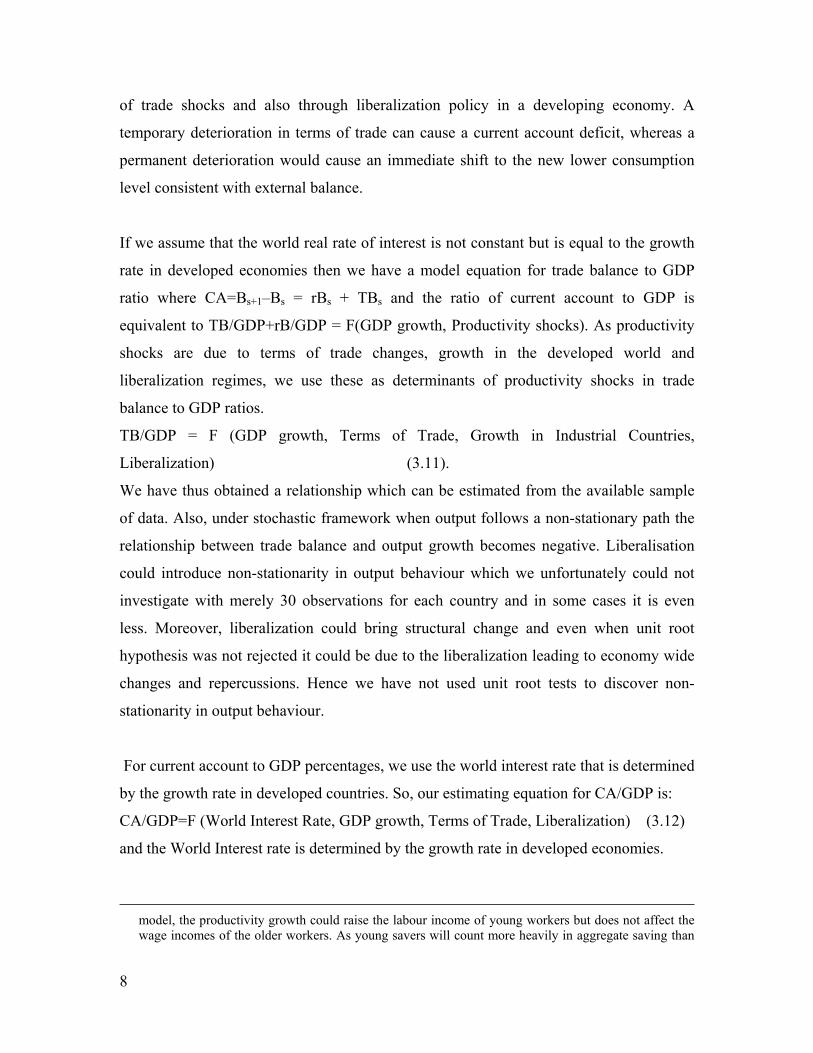
If we assume that the world real rate of interest is not constant but is equal to the growth

rate in developed economies then we have a model equation for trade balance to GDP

ratio where CA=Bs+1–Bs = rBs + TBs and the ratio of current account to GDP is

equivalent to TB/GDP+rB/GDP = F(GDP growth, Productivity shocks). As productivity

shocks are due to terms of trade changes, growth in the developed world and

liberalization regimes, we use these as determinants of productivity shocks in trade

balance to GDP ratios.

TB/GDP = F (GDP growth, Terms of Trade, Growth in Industrial Countries,

Liberalization) (3.11).

We have thus obtained a relationship which can be estimated from the available sample

of data. Also, under stochastic framework when output follows a non-stationary path the

relationship between trade balance and output growth becomes negative. Liberalisation

could introduce non-stationarity in output behaviour which we unfortunately could not

investigate with merely 30 observations for each country and in some cases it is even

less. Moreover, liberalization could bring structural change and even when unit root

hypothesis was not rejected it could be due to the liberalization leading to economy wide

changes and repercussions. Hence we have not used unit root tests to discover non-

stationarity in output behaviour.

For current account to GDP percentages, we use the world interest rate that is determined

by the growth rate in developed countries. So, our estimating equation for CA/GDP is:

CA/GDP=F (World Interest Rate, GDP growth, Terms of Trade, Liberalization) (3.12)

and the World Interest rate is determined by the growth rate in developed economies.

model, the productivity growth could raise the labour income of young workers but does not affect thewage incomes of the older workers. As young savers will count more heavily in aggregate saving than

9

In the above relationships, we expect interactions between liberalization and GDP growth

and liberalization and terms of trade. The marginal effect of GDP growth on TB/GDP

will be negative (or positive according to one view) as developing countries are likely to

grow faster than developed countries and their import propensity will be higher than

export propensity in the short-run. Moreover, the marginal impact of the terms of trade

will be positive as a favourable change in the terms of trade of developing economies will

lead to an improvement in TB/GDP ratio. The higher growth in developed economies

will improve the trade balance to GDP ratio as the developing countries are likely to

export more to the developed world (since growth in the industrialized world creates

demand for commodities and raw-materials including intermediate products).

4 Trade balance and growth relationships, structural change and Dynamic Panel

Models

We estimated a dynamic model with one and two lags and prefered the model with one

lag. All equations were estimated by Generalised Method of Moments. Before these

models were estimated we considered static panel data models (without lags) and

obtained estimates from fixed effects and random effects models6. We write the equation

for a dynamic model in the following form:

ittiitititit yyy εηαδδ +++++= −− BX2211 i = 1, 2…….42, t = 1,2,…….31 (4.1)

yit is the trade balance or current account to GDP in percentages, Xit is a set of

explanatory variables namely liberalization, growth in real GDP, purchasing power of

exports (terms of trade), and interactions of liberalisation with purchasing power of

exports and of liberalisation with the growth rate in real GDP in developing and

developed economies. ηt is the effects of time or year dummies and may be represented

as cyclical impacts on trade balance to GDP percentages. When the dependent variable is

old dissavers, saving will tend to rise and the current account to improve. (Obstfeld 1995).

6 Results of these can be obtained from the author. These models using panel data analysis differ accordingto whether they treat intercept parameters as random or fixed across the sample. The estimators in therandom effects model are the generalized least squares estimators, and they combine the within andbetween country estimators using the corresponding residual variances as weights. For elementary paneldata techniques see Johnston (1996). For special treatment of panel data models, see Baltagi (1995) andWooldridge (2002).

10

current account to GDP percentages, we use the debt related variables namely debt

service to payments ratios, annual growth in accumulated long-term debt and percentage

change in world interest rates7.

We expect the sign of the coefficients to be positive with respect to purchasing power of

exports and growth in developed economies while we expect negative sign with respect

to growth in real GDP and oil prices. Two-year lags are used on the assumption that lags

are not likely to be longer.

Even if yit-1 and εit are not correlated, and t does not approach infinity (t=31 in our case)

then estimation by fixed effects or random effects is not consistent even if n (number of

countries) goes to infinity. Arellano and Bond (1991) suggest an alternative procedure

that corrects not only for the bias introduced by the lagged endogenous variable, but also

permits a degree of endogeneity in the other regressors (such as Growth variable on the

right hand side variable as a subset of X matrix). The Generalized Method of Moments

Estimator first differences each variable and then uses the lagged values of each of the

variables as instruments. Specifically,

ititititit yyy εδδ ∆++∆+∆=∆ −− B∆X2211 (4.2)

The first three observations are lost due to lags and differencing. Assuming that εit are not

autocorrelated for each i at t=4, yi1 and yi2 are valid instruments for lagged variables.

Similarly, at t=5, yi1, yi2 and yi3 are valid instruments. We thus estimate the dynamic

model using the above procedure.8

7 We expect the current account to deteriorate with an increase in debt, increase in service payments and an

increase in world interest rates. Expected signs are negative with respect to each one of them.8 Monte Carlo simulation has shown that for panels with t=5 or 6, the bias of the coefficients of lagged

dependent variable can be significant, although the bias for the coefficients on other right hand sidevariables tends to be minor.

11

Results of Arellano-Bond Estimation on the Whole Sample for the Entire period and

sub-Periods

In Tables 2A, 2B and 2C, the results of dynamic models are presented for the period

1980-1999 using a sample data of 42 countries. The panel is unbalanced as we do not

have data for all the years for all countries. Data for earlier period were not consistently

available and hence we have excluded period 1970 to 1979. Our study is over the period

1980-1999. First differences remove the fixed effects and given the dynamics, we

introduce lagged effects on changes in TBGDP1 and CAGDP1 in respective trade

balance and current account equations. We sometimes, find that both growth and lagged

growth effects are negative on trade balance. (Table 2C). This also confirms that the

faster domestic growth effects trade balance adversely. Liberalisation increases current

account deficits as in Table 2A. Overall liberalisation deteriorates trade deficits but its

effects come through terms of trade interaction with liberalisation. In Table 2A,

liberalisation is used as a dummy and also a slope dummy where it is interacting with

income terms of trade. This means that liberalisation affects terms of trade and the terms

of trade with liberalisation has a negative impact on trade balance. In Table 2B, our

results indicate that liberalisation on its own has a negative impact although the

coefficient is not significant. Growth in developed world tends to improve trade balance

in developing countries while it tends to worsen current account balance according to

results of Table 2B. In Tables 2B and 2C time dummies are used while Table 2A does not

use time dummies. Time dummies indicate that there are autonomous effects and such

effects could be correlated with country-invariant advanced countries’ growth rates. The

terms of trade have significant positive effects on trade balance but interaction with

liberalisation variable has negative effect. (Table 2A).

5. Regional Analysis and Sub-Period Models

It might be worthwhile to look at the results by regions and by sub-periods. Is there any

evidence of change in the relationship between trade balance and economic growth

between different sub-periods? Our UNCTAD (1999) study demonstrated that the

12

relationship between trade balance and GDP growth could have changed from one decade

to the next. In order to study this aspect we shall examine the estimates of the periods

1980-89 and 1990-99 using the data of as many countries as possible in each of these

periods. It is the estimation based on panel data and we use the Blundell-Bond (1998)

dynamic panel estimator. We now do not estimate current balance to GDP equation. All

results refer to TBGDP1 and they are obtained using System GMM and equation GMM

as they are explained in Bond (2000). These results are presented in Tables 3A and 3B.

Terms of trade have significant effects on trade balance during 1980-89 period with the

two step system GMM. Growth variable does not have significant relationship with

TBGDP1 and this means that although the relationship is negative, it does not have

harmful effects on trade balance. (Table 3A) Liberalisation on its own does not have

significant impact on TBGDP1 during 1980-89 period. There seems to be significant

evidence that the relationship between trade balance and GDP growth is negative in

1990-2000 decade while although the relationship is negative, it is not significant for the

previous decade (Table 3B). Liberalisation is tending to have negative impact on

TBGDP1 during the period 1990-2000. We thus establish that some of the conclusions

we mentioned in Section 2 are valid according to the dynamic panel estimator.

Table 4 reports results for African countries for two sub-periods 1980-89 and 1990-99.

For the first period, all time dummies were insignificant. We have an unbalanced panel

but when observations are differenced out we have very few observations for each decade

of 1980-89 and 1990-2000. The lagged dependent variable has a small coefficient

although significant. The sign of growth variable for 1990-2000 decade is negative and

significant but not for 1980-89 period. Liberalisation has a negative and significant

coefficient for the 1990-2000 period and an increase in liberalization may lead to 1.95

percentage point decline in trade balance. For the first period, advanced countries’ growth

has a significant role to play in improving trade balance. Overall, we find that the

relationship is different between two periods and our hypothesis about liberalization9 and

9 We used other variations of the equations for Current account and Trade balancevariables. Growth was never significantly related to trade balance or current account inthe first period. Liberalisation has reduced both trade account and current accountbalances in Africa in the period 1990-2000. The dominant negative effect on tradebalance comes from its interactions with terms of trade. Liberalisation may deteriorate

13

domestic growth both having deteriorating impacts on trade balance in the 1990-2000

time period, is confirmed.

In Table 5, we use the entire sample for African and Latin American economies. For

African economy, growth in advanced country plays a positive and significant role in

improving trade balance. This may imply that the behaviour overall is very different

between two periods. For Latin American economies, growth has a negative impact on

trade balance; an increase in income terms of trade improves trade balance, liberalization

is not significant and dynamic model is plausible. Many time dummies for Latin

America are significant so there is a great deal of autonomous effect on trade balance and

as anticipated, the effect is positive up to 1988 and as we mentioned before this was the

period when both trade balance and economic growth improved. The decade of 1990 for

Latin America10 shows a worsening of trade balance and this is captured to some extent

in time dummies.

In Table 6, we provide results of Latin American trade balance equations for two

different periods. We find that the growth coefficients are not significant for the first

period while for the second period they are highly significant and negative suggesting

that growth deteriorates trade balance. The growth in advanced countries improves trade

balance in Latin American and Asian economies. Terms of trade have positive impact on

trade balance in both periods while liberalization on its own is not significant in either

period. Again when two periods are studied separately and with the first differencing the

number of observations is small. Our System-GMM did not produce significant results on

a large number of variables.

terms of trade as imports expand at a faster rate and import prices might rise faster thanexport prices leading to deterioration in terms of trade and this in turn could lead to tradebalance deterioration. For African economies, liberalisation interacting with growth has apositive impact on trade balance.10 We only considered trade balance to GDP and two models, one with time dummies andanother without time dummies are estimated. Growth is significantly negatively related totrade balance in both models. What we can infer here is that faster economic growth inAsian and Latin American countries would lead to a decline in trade balance as importgrowth far exceeds export growth. Surprisingly, growth in advanced countries does notremove pressure on trade balance or current account balance.

14

6. Summary and Conclusion:

One of the major issues is the capital financing requirements in the presence of trade

deficits in the short and medium run for developing economies. Globalisation has made

both developing and developed countries highly interdependent. If developing countries

were to catch up with developed countries in their per capita income, enormous help from

developing countries may be needed from developed countries by way of capital

financing. Our study seems to indicate that there are differing patterns on trade deficits

across various geographical regions and also during the decade of 1990-1999. Trade

liberalization has increased the imports of many developing countries and although after

initial phase of import growth exports picked up in some developing countries, on the

whole, it remained insufficient to narrow the trade deficits. Rapid liberalisation was

sometimes followed by large inflows of capital, currency appreciation and mounting

trade deficits, but it often ended up with a crisis involving reversal of capital inflows,

collapse and overshooting of exchange rates, sharp cuts of imports and a deep economic

contraction.

We find that trade liberalization does have significant relationship with economic growth

and/or trade deficits in short to medium-run. Current account deficits have sometimes

increased because of trade liberalization in African economies during the period 1980-

1999. Our significant relationship between liberalization and trade deficits and economic

growth and trade deficits is for Latin American and Asian economies for the latter

decade. This seems to indicate that their capital financing requirements are much higher

than the world community has been able to provide and rapid liberalization has often

caused financial crisis and debt problems in Latin American and some Asian economies.

Our study has many limitations as the data inadequacies dominate the model estimation.

The measures of trade liberalization such as Sachs-Warner (1995) or Wacziarg (2001) do

not take into account different intensities of liberalization in different time periods. Our

study has not considered liberalization attempt by any developed economy. Tariff and

non-tariff barriers on a significant scale exist in developed countries for agricultural

products emerging from developing economies.

15

References

Arellano, M. and Bond, S. R. (1991), ‘Some Tests of Specification for Panel Data: MonteCarlo Evidence and an Application to Employment Equations’, Review of EconomicStudies, Vol.58, pp.277–97.

Baltagi, B. (1995), Econometric Analysis of Panel Data, John Wiley & Sons.

Blundell R. and Bond S. (1998) ‘Initial Conditions and Moment Restrictions in DynamicPanel Data Models’, Journal of Econometrics, 87, 115-143

Bond, S. ‘Dynamic Panel Data Models: A Guide to Micro Data Methods and Practice’Institute of Fiscal Studies, London, Paper 09/02.

International Monetary Fund, World Economic Outlook, various issues.

Johnston, J. (1996), Econometric Methods, New York: McGraw Hill.

Obstfeld, M. (1995), ‘The Intertemporal Approach to the Current Account’, Chapter 34 inHandbook of International Economics, Vol.III, edited by G. Grossman andK. Rogoff, Elsevier Science B.V.

Obstfeld, M. and Rogoff, K. (1997), Foundations of International Macroeconomics,Cambridge MA: Academic Press.

Parikh, A. and Stirbu, C. (2004), Relationship Between Trade Liberalisation, EconomicGrowth and Trade Balance: An Econometric Investigation”, HWWA Discussion PaperNo. 282, Hamburg Institute of International Economics, Hamburg,1-50

Sachs, J. and Warner, A. (1995), ‘Economic Reform and the Process of GlobalIntegration’, Brookings Papers on Economic Activity, Vol.1, pp.1–118.

UNCTAD (1999), Trade and Development Report, United Nations, Geneva, Switzerland.

Wooldridge, J. M. (2002), ‘Econometric Analysis of Cross Section and Panel Data’,Cambridge MA.

Wacziarg, R. (2001), “Measuring the dynamic gains from trade”, World Bank EconomicReview, Vol. 15 (3), pp. 393-429.

World Bank (1998), “Global Economic Perspectives 1998/99“, Washington DC: WorldBank.

16

Table 1Trade account to GDP ratio and GDP growth: 1989–96 compared with 1982–88

Improving trade account Deteriorating trade account

More than 10% 5 to 10% 2 to 5% 0 to 2% 0 to 2% 2 to 5% 5 to 10% More than 10%More than5% growth

Syria Libya Iran GuineaGuyana

Sudan

3 to 5% PNGSingapore

JordanTrinidadandTobago

Gabon Argentina Bolivia GuatemalaLiberiaMalaysiaNicaraguaPhilippinesUganda

El Salvador

1 to 3% BeninNigeria

SaudiArabia

Mali Niger Ecuador ChileFijiIndonesiaPeruThailand

KuwaitMexico

MauritaniaTanzania

RisingGrowth

0 to 1% Venezuela BangladeshColombiaSri LankaTunisia

Cote d'Ivorie DominicanRep.HondurasJamaicaNepal

Paraguay

FallingGrowth

0 to 1% Guinea Bissau Congo CARChinaSenegal

India Costa RicaZambia

Malawi Ghana

1 to 3% Burkina Faso Pakistan AlgeriaCyprusMorocco

BrazilKenyaTurkey

Hong KongKoreaMadagascar

MauritiusZimbabwe

Gambia

3 to 5% Chad Togo BarbadosEgyptHaiti

Sierra Leone Taiwan

More than5%

Cameroon Iraq BotswanaDemocraticRep of CongoRwanda

Burundi

18 big countries in bold (defined as largest GDP in 1990-95 and GDP greater than US $60 billion in 1997 excluding the major oil-exporting countries, as well as Hong Kong,Singapore). 9 major oil exporting countries in italics. 9 main exporters of manufactures underlined.All data from ETS except data on current GDP are from World Development Indicators for Ghana, India, Jamaica, Malaysia, Mauritania, Nigeria, Papua New Guinea, Rwanda, SierraLeone, Sri Lanka, Thailand, Trinidad and Tobago, Zimbabwe. As no data on current GDP are available for 1996 for Barbados, Bolivia, Gambia, Iran, Iraq, Liberai, Libya, Saudi Arabiaand Sudan, the second period comprises only 1989–95 for these countries.

17

Table 2A

Regression Coefficients, Z-statistic: Arellano-Bond Dynamic Panel Estimation 1980-99(42 countries Unbalanced Panel)

TBGDP1 CAGDP1Name of theVariable

Coefficient Z-statistic Coefficient Z-statistic

TBGDP(-1) 0.7335*** 29.44CAGDP(-1) 0.5198*** 8.00GROWTH -0.0346* -1.93 0.0020 0.12LIBGROWTH 0.0129 0.43PPI 0.0142*** 3.35 0.0021 1.69LIBER 0.3167 0.54 -0.3442* -1.90LIBPPI -0.0104** -2.35ADVGR 0.0018 0.14 0.0234*** 3.02DEBTSR 1.3365 0.78GLTDOL -0.0058** -2.12CINTEREST 0.0025 1.91CONSTANT 0.0489** 2.76 0.0373** 2.78First Order AC -12.94 (0.000) -3.04 (0.0024)Second OrderAC

1.88 (0.0604) 1.22 (0.2208)

Wald χ2 247.98 (8 DF)Number of Obs 888 849Sargan Test χ2 655.35 (0.00)Time Dummies are not used.***Significant at 1% level, **Signficant at 5% level, *Significant at 10% level

18

Table 2BRegression Coefficients, Z-statistic of Arellano-Bond Dynamic Panel Estimation 1980-99(42 countries Unbalanced Panel) WITH TIME DUMMIES

TBGDP1 CAGDP1Name of theVariable


TBGDP(-1) 0.7406*** 20.83CAGDP(-1) 0.4665*** 8.56GROWTH -0.0264 -1.20 0.01236 0.64GROWTH(-1)PPI 0.0058*** 3.64 0.0024 1.61LIBER -0.5860 -1.39 -0.2705 -0.79ADVGR 0.0161 0.61 -0.5655** -2.28LIBGROWTH -0.0062 -0.18DEBTSR 1.4278 0.90GLTDOL 0.0053 0.77CINTEREST 0.0618** 2.31CONSTANT 1.6625** 2.33First Order AC -8.80(0.000) -3.75(0.0002)Second OrderAC

1.69(0.0906) 0.72 (0.4687)

Wald χ2 698.67 (22DF) 1474.70 (23DF)Number of Obs 537 692Sargan Test χ2 322.96(0.000)Year Dummies used.***Significant at 1% level, **Signficant at 5% level, *Significant at 10% level

19

Table 2CRegression Coefficients, Z-statistic of Aralleno-Bond Dynamic Panel Estimation 1980-99(42 countries Unbalanced Panel) WITH TIME DUMMIESTBGDP1 CAGDP1Name of theVariable


TBGDP(-1) 0.7028*** 6.16CAGDP(-1) 0.4436*** 7.92GROWTH -0.0360 -1.32 -0.0123 -0.64GROWTH(-1) -0.0335** -2.23 0.0039 0.45PPI 0.0141** 2.79 0.0072** 2.38LIBER 0.7189 1.10 0.4942 1.08LIBPPI -0.0053* -1.79ADVGR 0.0569** 2.17 0.0266 1.31ADVGR(-1) -0.1083 -3.61 -0.0733*** -3.08LIBGROWTHDEBTSR 1.2015 0.79GLTDOL 0.0062 0.95CINTEREST 0.0025 0.84CONSTANT 0.0351 0.53 0.1315** 2.22First Order AC -3.10 (0.0019) -3.82 (0.0001)Second OrderAC

1.07 (0.2845) 0.71 (0.48)

Wald χ2 359.03 (23 DF) 3025.52 (25DF)

Number of Obs 537 692Sargan Test χ2

Year Dummies used.***Significant at 1% level, **Signficant at 5% level, *Significant at 10% level

20

Table 3ABlundell-Bond Dynamic Panel Estimators with System GMM and Difference GMM forTBGDP1 of 42 Countries, 1980-1989System GMM DIFF-GMMName of theVariable

Coefficient t-statistic Coefficient t-statistic

TBGDP(-1) 0.9127*** 20.49 0.7017*** 3.41GROWTH -0.0400 -1.52 -0.0263 -1.24PPI 0.0109*** 2.12 0.0093 1.37ADVGR 0.0777 1.61 0.1101 3.28LIBER -1.2012 -1.20 -0.8278 -0.89Year81 -0.3207 -0.41 0.1045 1.12Year82 1.3381 1.66 1.6162*** 3.20Year84 0.1346 0.36 0.3341 0.84Year85 0.4103 0.92 0.8166** 2.03Year86 0.5796 0.90 1.2355*** 3.33Year88 -0.6310 -1.75* -0.4255 -1.28Year89 0.2055 0.49 0.1876 0.47Constant -1.0411 -1.58 ------AR(1) -2.76(0.006)*** -2.31 (0.021)***AR(2) 1.05(0.294) 1.09 (0.274)Hansen Test χ2(101)=26.87(1.00) χ2(96)=23.68(1.00)No. of Obs. 301 259

*** Significant at 1% level; **Significant at 5% level, *Significant at 10% level

Notes:

1. Year dummies are included in the second period and as they were insignificant inthe first period, they were excluded.

2. Asymptotic standard errors, asymptotically robust to heteroscedasticity arereported in parentheses.

3. First order AC and second order AC are tests of first-order and second-order serialcorrelation in the first differenced residuals, asymptotically distributed as N(0,1)under the null of no serial correlation.

4. Sargan is a test of over-identifying restrictions, asymptotically distributed as χ2

under the null of instrument validity, with degrees of freedom reported inparentheses.

5. The instruments used in each equation are: GMM (DIF)- TBGDPit-2….TBGDPi1,GROWTHit-1….GROWTHi1, PPIit-1…..PPIi1 and ADVGRit-1…..ADVGRi1

21

Table 3BBlundell-Bond Dynamic Panel Estimators with System GMM and Difference GMMfor TBGDP1 of 42 Countries, 1990-2000System GMM DIFF-GMMName of theVariable


TBGDP(-1) 0.9439*** 13.98 0.5016*** 5.38GROWTH -0.0862* -1.72 -0.1214*** -2.66GROWTH(-1) -0.0423 -0.82 -0.1011*** -3.70PPI 0.0053*** 3.17 0.0068** 2.36ADVGR 0.0054 0.17 -0.0287 -1.28LIBER -1.2442 -1.13 -1.1325 -1.55Year2 -0.3207 -0.41 -0.1405 1.39Year3 1.3381 1.66 -0.2950 -0.74Year4 0.1346 0.36 -0.3708 -1.28Year5 0.4103 0.92 0.5598* 1.75Year6 0.5796 0.90Year7 0.3268 0.95Year8 -0.6310 -1.75*Year9 0.2055 0.49 0.0695 0.22Year10 -0.1174 -0.20 0.0965 0.21Constant -1.0411 -1.58 ------AR(1) -2.76(0.006)*** -2.59 (0.01)***AR(2) 1.05(0.294) -1.05(0.293)Hansen Test χ2(101)=26.87(1.0

0)χ2(112)=19.54(1.00)

No. of Obse 301 226

*** Significant at 1% level; **Significant at 5% level, *Significant at 10% levelNotes:






5. The instruments used in each equation are: GMM (DIF)- TBGDP1it2….TBGDP1i1,GROWTHit-2….GROWTHi1, PPIit-1…..PPIi1 and ADVGRit-1…..ADVGRi1. Insystem-GMM, the above instruments are used in the differenced equations and∆TBGDP1it-1, ∆GROWTHit-1, ∆ADVGRit-1, and ∆PPIit-1

22

Table 4

Regression Coefficients, t-statistic of Bond-Blundell Dynamic Panel Estimation 1980-2000: AFRICA: With or Without Time Dummies

TBGDP1:1980-89 TBGDP1 1990-2000One Step DIF-GMM One Step DIF-GMM

Name of theVariable


TBGDP(-1) 0.3494*** 3.92 0.2903* 1.73GROWTH -0.0073 -0.26 -0.0718 -1.52GROWTH (-1) -0.0115 -0.42 -0.1128** -2.31PPI 0.0176** 2.57 -0.0004 -0.12LIBER -0.3272 -0.60 -1.9490** -2.42ADVGR 0.0716** 2.06 0.0253 0.56Year 92 -1.3665** -2.20Year 93 -1.6351** -2.77Year 94 -0.3903 -0.66Year 96 -0.1397 -0.17Year 97 -0.1139 -0.17Year 98 -1.0755* -1.70Year 99 0.2431 0.36CONSTANT ---- ---- ------ -----First Order AC -2.92 (0.004) -1.40 (0.162)Second OrderAC

-1.12 (0.26) -0.16 (0.871)

Number of Obs 77 35Sargan Test χ2 76.68(0.115) 46.89

***Significant at 1% level, **Significant at 5% level and * Significant at 10% levelNotes:






10. The instruments used in each equation are: GMM (DIF)- TBGDPit-2….TBGDPi1,GROWTHit-2….GROWTHi1, PPIit-1…..PPIi1 and ADVGRit-1…..ADVGRi1

23

Table 5 : Regression Coefficients, t-statistic Bond-Blundell Dynamic PanelEstimation: AFRICA and Latin America for 1980-2000

AFRICA LATIN AMERICAName of theVariable


TBGDP(-1) 0.6066*** 9.34 0.6769*** 6.00GROWTH 0.0105 0.42GROWTH(-1) -0.0033 -0.14 -0.0700*** -4.11PPI 0.0038 0.99 0.0062*** 3.31LIBER -0.4239 -0.77 -0.0717 -0.27ADVGR 0.1185** 2.38 0.0285* 1.71Year 3 1.9878*** 3.79Year 4 1.2090** 2.93Year 5 1.9316** 2.81Year 6 1.6710*** 3.42Year 7 1.7521*** 3.90Year 8 1.1654** 2.25Year 9 1.6514*** 4.29Year 10 0.8303** 2.68Year 13a -1.4840** -1.97CONSTANT 0.0088 0.15First Order AC -4.36 (0.000)Second OrderAC

1.14 (0.255)

Number of Obs 139Sargan Test χ2 131.23 (0.064)

a Only significant year effects are reported ***Significant at 1% level, **Significantat 5% level, *Significant at 10% levelNotes:

1.Year dummies are included in the second period and as they were insignificant inthe first period, they were excluded.2.Asymptotic standard errors, asymptotically robust to heteroscedasticity are reportedin parentheses.3.First order AC and second order AC are tests of first-order and second-order serialcorrelation in the first differenced residuals, asymptotically distributed as N(0,1)under the null of no serial correlation.4.Sargan is a test of over-identifying restrictions, asymptotically distributed as χ2

under the null of instrument validity, with degrees of freedom reported in parentheses.5.The instruments used in each equation are: GMM (DIF)- TBGDPit-2….TBGDPi1,GROWTHit-2….GROWTHi1, PPIit-1…..PPIi1 and ADVGRit-1…..ADVGRi1

24

Table 6Regression Coefficients, t-statistic Bond-Blundell Dynamic Panel Estimation 1980-99: Latin America and AsiaTBGDP1: 1980-1989: DIF GMM TBGDP1:1990-2000:DIF GMMName of theVariable


TBGDP(-1) 0.7473*** 4.90 0.5066*** 8.49GROWTH -0.0547 -1.41 -0.1679*** -3.65GROWTH(-1) -0.0377 -1.28 -0.0905** -2.62PPI 0.0103** 2.04 0.00985*** 4.87LIBER -0.7098 -1.10 0.8669 1.22ADVGR 0.1278*** 3.44 -0.0408 1.65CONSTANT 0.1078 1.34 -0.2158** -2.21First Order AC -2.22 (0.027) -2.46 (0.014)Second OrderAC

1.46 (0.145) -0.43 (0.668)

Number of Obs 182 177Sargan Test χ2 10.63 (1.00) 10.35 (1.00).***Significant at 1% level, **Significant at 5% level, *Significant at 10% levelNotes: 1. Year dummies are included .

2. Asymptotic standard errors, asymptotically robust to heteroscedasticity are reportedin parentheses.3. First order AC and second order AC are tests of first-order and second-order serialcorrelation in the first differenced residuals, asymptotically distributed as N(0,1)under the null of no serial correlation.4. Sargan is a test of over-identifying restrictions, asymptotically distributed as χ2

under the null of instrument validity, with degrees of freedom reported in parentheses.5. The instruments used in each equation are: GMM (DIF)- TBGDPit-2….TBGDPi1,GROWTHit-2….GROWTHi1, PPIit-1…..PPIi1 and ADVGRit-1…..ADVGRi1

relationship between trade liberalisation, growth and...

Documents