relationship between physico-chemical conditions...
TRANSCRIPT

RELATIONSHIP BETWEEN PHYSICO-CHEMICAL
CONDITIONS AND PHYTOPLANKTON VARIABILITY IN ALFACS BAY
Author: OIHANE MUÑIZ PINTO
Director: ELISA BERDALET I ANDRES
Additional supervision: NORMA ZOE NESZI
Centre: Institut de Ciències del Mar (ICM-CSIC). Departament de Biologia Marina & Oceanografia
Màster en Ciències del Mar: Oceanografia i Gestió del Medi Marí
September 2012


ACKNOWLEDGMENTS
I am grateful to the University of Barcelona and the ICM-CSIC for giving
master's students the opportunity to get to know what working on a research
project means. It has been a really positive and enriching experience.
I would also like to thank my supervisor Norma Zoe Neszi, for all that she
taught me, and Elisa Berdalet for her help, support and knowledge.
And finally, I am really grateful to my parents and friends, for their patience
and encouragement.

ABSTRACT
Understanding the spatio-temporal variability of phytoplankton in
aquaculture areas is necessary for the appropriate management of natural
resources and the prevention of noxious outbreaks. With this objective in mind,
we conducted weekly samplings during the spring of 2011 in Alfacs Bay, a
microtidal estuary in the NW Mediterranean and an important area of shellfish
and finfish explotation which is regularly affected by toxic outbreaks. The study
was part of the ECOALFACS project (CTM2009-09581), and here we focus on
the results obtained during 4 consecutive weeks (May 31st to June 21st). We
describe the main water column properties (temperature, salinity and inorganic
nutrient composition) and phytoplankton community composition.
CTD casts revealed that the water column was initially well mixed,
subsequently stratified during the 2nd and 3rd weeks, and mixed again in the last
sampling. Over the studied period, temperature increased but the salinity
variation remained within the range characteristic of this embayment where
freshwater supply occurs at surface from irrigation channels from the nearby
delta rice fields. Inorganic nutrients were very low, specially phosphorus, which
was close to the detection limit. Silicate tended to increase towards the second
half of the studied period. Likely due to such limiting nutrient conditions,
chlorophyll values remained pretty similar, with values no exceeding the 4 µg·L-
1. The organisms smaller than 5µm contributed by more than the 50% of the
total biomass, specially towards the end of the studied period.
The succession of the main phytoplankton groups indicated that the spring
diatom bloom was decaying during the 1st weeks of our study, with flagellates
dominating over dinoflagellates and diatoms. The most relevant differences
among the microphytoplankton organisms was due to particular dinoflagellate
taxons.

RESUMEN
Es importante entender la variabilidad espacio-temporal del fitoplancton
en zonas de acuicultura para una apropiada gestión de los recursos naturales y
la prevención de brotes nocivos. Con este objetivo, llevamos a cabo muestreos
semanales durante la primavera del 2011 en la bahía dels Alfacs, un estuario
micromareal en el Mediterráneo noroccidental e importante zona de mariscos y
explotación de peces que es regularmente afectada por brotes tóxicos. Este
estudio es parte del proyecto ECOALFACS (CTM2009-09581), y nos
centramos en los resultados obtenidos durante 4 semanas consecutivas (31 de
Mayo - 21 de Junio). Describimos las principales propiedades de la columna de
agua (temperatura, salinidad y composición de nutrientes inorgánicos) y la
composición de la comunidad fitoplanctónica.
Los datos obtenidos con el CTD revelaron que, inicialmente, la columna
de agua estaba mezclada, posteriormente estratificada durante la 2ª y 3ª
semana, y mezclada de nuevo en el último muestreo. La temperatura aumentó
durante el período estudiado, pero la variación de la salinidad se mantuvo
dentro del rango característico de esta ensenada, debido a los aportes
superficiales de agua dulce procedente de los canales de riego de los campos
de arroz del delta. Las concentraciones de nutrientes inorgánicos fueron muy
bajas, especialmente las de fósforo, que se encontraba cerca del límite de
detección. El silicato tendió a aumentar en la segunda mitad del período
estudiado. Los valores de clorofila se mantuvieron bastante similares, con
valores que no excedieron los 4 µg·L-1, probablemente debido a la limitación
por nutrientes. Los organismos inferiores a 5 µm contribuyeron en más del 50%
de la biomasa total, especialmente hacia el final del período de estudio.
La sucesión de los principales grupos de fitoplancton indicó que el bloom
primaveral de diatomeas fue decayendo durante las primeras semanas de
estudio, pasando a un dominio de los nanoflagelados sobre los dinoflagelados
y las diatomeas. Las diferencias más relevantes entre los organismos
microplanctónicos fue debida a taxones concretos de dinoflagelados.

RESUM És important entendre la variabilitat espai-temporal de fitoplàncton en
zones d’aqüicultura per a una apropiada gestió dels recursos naturals y per la
prevenció de brots nocius. Amb aquest objectiu portem a terme mostres
setmanals durant la primavera del 2011 a la badia dels Alfacs, un estuari
micromareal en el Mediterrani nort-occidental i a més a més, una zona
important de mariscs y explotació de peixos, la qual és regularment afectada
per brots tòxics. Aquest estudi és part del projecte ECOALFACS (CTM2009-
09581), i ens centrem en els resultats obtinguts durant quatre setmanes
consecutives (31 Maig – 21 Juliol). Descrivim les principals propietats de la
columna d’aigua (temperatura, salinitat y composició de nutrients inorgànics) y
la composició de la comunitat fitoplanctònica.
Les dades obtingudes amb el CTD van deixar veure que, inicialment, la
columna d’aigua estava barrejada, posteriorment estratificada durant la segona
i la tercera setmana i barrejada de nou en l’ últim mostreig. La temperatura va
augmentar durant el període estudiat, però la variació de la salinitat es va
mantindre dins la franja característica d’aquesta badia, degut a les aportacions
superficials d’aigua dolça procedent dels canals de reg dels camps d’arròs del
Delta. Les concentracions de nutrients inorgànics van ser molt baixes,
especialment les de fòsfor, que es trobava a prop del límit de detecció. El silicat
va tendir a augmentar en la segona meitat del període estudiat. Els valors de
clorofil·la es van mantindre bastant similars, amb valors que no es van extendre
dels 4 ug·L-1, probablement va ser degut a la limitació per nutrients. Els
organismes inferiors a 5 µm van contribuir en més del 50% de la biomassa
total, especialment fins al final del període d’estudi.
La successió dels principals grups de fitoplàncton va indicar que el
bloom primaveral de diatomees va anar de cap a caiguda durant les primeres
setmanes d’estudi , passant a un domini dels nanoflagelats sobre els
dinoflagelats i les diatomees. Les diferències més rellevants entre els
organismes microplanctonics va ser deguda a taxones concrets de
dinoflagelats.

INDEX
1. Introduction .................................................................................................. 1
1.1. Alfacs bay ......................................................................................... 1
1.2. Phytoplankton in Alfacs bay ............................................................. 2
1.3. Harmful Algal Blooms (HABs) .......................................................... 4
1.4. Objective .......................................................................................... 4
2. Material and methods .................................................................................. 5
2.1. Cruises ............................................................................................. 5
2.2. CTD casts ......................................................................................... 5
2.3. Weather conditions ........................................................................... 5
2.4. Sampling .......................................................................................... 5
2.5. Nutrients ........................................................................................... 6
2.6. Chlorophyll ....................................................................................... 6
2.7. Microphytoplankton .......................................................................... 7
2.8. Nanophytoplankton and cyanobacteria ............................................ 8
3. Results ........................................................................................................ 10
3.1. CTD casts and weather conditions ................................................. 10
3.2. Nutrients and cholorophyll .............................................................. 13
3.3. Microphytoplankton ........................................................................ 15
3.4. Nanophytoplankton and cyanobacteria .......................................... 19
4. Discussion .................................................................................................. 20
5. Conclusions ............................................................................................... 24
6. References .................................................................................................. 26

1
1. INTRODUCTION
1.1. Alfacs Bay
Alfacs is a shallow bay situated in the south of the Ebro delta (NW
Mediterranean sea 40º40'N, 0º40'E) (Fig.1). This semi-enclosed estuary is
separated from the Mediterranean by a sand barrier that leaves a 2500 m
wide opening to the open sea. The total area of the bay is about 49 km2 with a
maximum depth of 6.5 m at the center of the bay (mean depth of 3.13 m)
(Camp et al. 1992).
As other estuarine environments, it is an ecosystem with high biological
productivity that provides important resources and socio-economical services:
this area is considered a successful fish and shellfish aquaculture site
(Colomé et al. 1997), as it is Catalunya's biggest fishing harbour. Thus, it is
exposed to both natural and anthropogenic stresses. In one hand, climatic
factors drive the short-term variability, while freshwater inputs of
anthropogenic origin result in a yearly cycle (Llebot et al. 2011; Vidal et al.
1997).
Fig. 1. Map of the area of study. The x shows the Raft Station. (Llebot et al. 2011)

2
Compared to the adjacent Mediterranean waters, the productivity of Alfacs
bay is high, due to the freshwater input from the rice fields of the delta. This
freshwater runoff contains a high concentration of inorganic nitrogen but a
very low concentration of phosphorous, most likely due to its retention on the
rice fields (Llebot et al. 2010). Therefore, phytoplankton growth in the bay is
usually phosphorus limited (Mura et al. 1996).
The freshwater inflow creates a stratification that dominates over tidal
mixing, which is lower than 0.2 m (Llebot et al. 2011), yielding a strongly
stratified, two layered system. In this situation, the main flow is characterized
by a classical estuarine circulation pattern (Camp 1994), where marine water
enters at lower depth and freshwater flows out at the surface (Camp 1994;
Dyer 1979 in Camp and Delgado 1987; Llebot et al. 2011). Solé et al. (2009)
described two basic states for the bay’s hydrography: a) one transient state of
a short period (2-5 days) consisting of the mixing of the water column caused
by storm events or winds stronger than 4.5 m·s-1; b) a steady state that
maintains the estuarine typical dynamics (stratification, salt-wedge) almost all
the year. This steady state presents three periods: open channel period (from
April to September), semi-open period (from October to December) and
closed channel period (from January to March/April). The alternation between
stratification and mixing depends on three main factors: freshwater input, wind
forcing and solar radiation (Camp and Delgado 1987).
1.2. Phytoplankton in Alfacs Bay
Climatologic studies performed by Solé et al. 2009 showed a seasonal cycle
in the bay due to climatic forcing. Solar radiation, for instance, is the major
drive of the phytoplankton annual cycle, whereas its short-term variability is
given by factors related to the water column motion. In other words, variability
of the physical conditions is a major factor controlling the dynamics of the
phytoplankton communities. Thus, understanding the coupling between
environmental and biological variables is an important research topic in this
productive area, and it will be a major objective of the present study.
In this line, most studies performed in Alfacs Bay have focused on
microphytoplankton, especially diatoms and dinoflagellates, which have been

3
recorded over almost 20 years (IRTA monitoring program) using the Utermöhl
(1958) method (e.g. Delgado et al. 2004; Fernández-Tejedor et al. 2008). This
is highly due to the fact that several dinoflagellates are involved in recurrent
harmful events that threaten aquaculture (Garcés et al. 1999). Those two
groups show different ecological strategies as it was illustrated in the
Margalef’s Mandala (Margalef 1978; Annex Fig. 1). In this conceptual frame,
different phytoplankton biologic types occur as an adaptation of the species to
a double gradient of nutrient concentration and turbulent kinetic energy
(Margalef 1980). Hence, in temperate latitudes, dinoflagellates are supposed
to be abundant in summer-autumn due to high radiation and warm
temperatures, and are usually the most numerous group in stratified and
nutrient poor waters (K strategy). This ability is due to their capacity for
mobility. In contrast, diatoms follow an R strategy, they respond fast to high
nutrient concentrations. Although they have mechanisms to diminish sinking
(small size, morphology), turbulence is decisive for diatoms in order to avoid
their sinking (e.g. Lalli and Parsons 1997, Vila and Masó 2005). Therefore,
during summer we would expect to find dinoflagellate's blooms as a property
of these coastal enriched waters, while diatoms would be associated with
winter and spring, where there is no stratification and relatively high nutrient
concentration (Vila and Masó 2005).
However, there is no information in Alfacs Bay about the smaller
components of the phytoplankton community, namely flagellates (or
nanoflagellates: NF), that can play an important role along the succession of
the different phytoplankton taxons, including the harmful species. NF
population represents an important link in the microbial food web.
Heterotrophic Nanoflagellates (HNF) are grazers, and they consume bacteria
and picophytoplankton. This trophic relationship is an essential link in the
transfer of carbon (C) to higher trophic levels. HNFs are also involved in
nitrogen (N) regeneration through microheterotrophic activity. Autotrophic
Nanoflagellates (ANF) carry out photosynthesis and that is why they are
essential components among the primary producers (Safi and Hall 1997). We
decided to include the NFs in this work because of the lack of information
regarding this group in Alfacs bay so far.

4
1.3. Harmful Algal Blooms (HABs)
Alfacs bay, due to high nutrient loads and high water residence times, favors
the development of phytoplankton communities. Sometimes, excess biomass
causes ecosystem damage (water discoloration, water quality deterioration)
because of the hypoxic conditions when decomposing. Some species
produce potent toxins that can be bioaccumulated in shellfish, which in turn
constitute a health risk to humans if consumed. These events often take place
in confined waters. All in all, the exploitation of the Catalan coastline shows an
increment in man-made sheltered waters resulting in more than 40 harbours
along 400km of coast. Each of those harbours is a modified shallow
ecosystem having reduced turbulence, high water residence times and high
nutrient concentration, what means a suitable condition for the proliferation of
phytoplankton, including harmful species (Vila et al. 2001). However, the
dynamics of HABs is very complex as it involves interactions among physical,
chemical, biological and ecological processes that operate at different spatio-
temporal scales (Chang and Dickey 2008). In Alfacs several toxic species are
harmful, and will lead to closure of the bay even if they are present at low
concentrations. For example, Dinophysis spp. will cause the closure of the
shellfish explotation at only 100 cells·L-1 and Alexandrium minutum at 100
cells·L-1. Given the importance of these phenomena known as Harmful Algal
Blooms (HABs) that cause both ecological and economic problems (GEOHAB
2001) it is so important investigating the general dynamics of phytoplankton,
and in particular that of the harmful species.
1.4. Objective
The objective of this work was to improve our comprehension of the physico-
chemical and biological conditions along the development of the
phytoplankton community in Alfacs Bay in spring. In order to understand the
variability and possible links among the environmental and biological
processes, weekly samplings were performed from March to July within the
context of the ECOALFACS project CTM2009-09581. Nevertheless, the
present study focuses on the 31st May to 21st June period at a central station
only. Our aim was to analyze the relatively small spatio-temporal scale
5
variability on the physico-chemical (temperature, salinity, inorganic nutrients)
water properties and to explore whether this variability affected the vertical
distribution and the temporal succession of the main phytoplankton groups. A
particular attention was devoted to track the presence of harmful
phytoplankton taxons, in order to understand whether the observed variability
could explain their presence or absence in the studied period.
2. MATERIAL AND METHODS
2.1. Cruises
During spring 2011 four weekly cruises (May 31st, June 7th, June 14th and
June 21st) were made at the Raft Station (40º 35’398 N, 000º 39’506 E), using
an 8 m boat.
2.2. CTD Casts
A SAIV A/S SD204 STD (Annex Fig.2) was lowered manually from surface
to the bottom (0 - 6 m approximately). The shallowest 0,2 m were not taken
into account for data analysis, because the sensors may not be completely
submerged. The CTD carried optional sensors for fluorescence, turbidity and
oxygen. Unfortunately, the oxygen sensor did not work in the first week and
the fluorescence sensor did not work in weeks 2 and 3. Data download and
export was performed with Minisoft SD200W and graphs were created with
Surfer 10.
2.3. Weather Conditions
For the weather description, in situ observations and meteorological data
from the Servei Meteorològic de Catalunya (SMC) were combined. The SMC
is stationed at the IRTA parking space, at 2 m height and gives continuous
data, sampling every hour.
2.4. Sampling
Samples for the estimation of nutrients, chlorophyll concentrations and
phytoplankton were collected every meter (from 0,5 to 5,5 m) with a low

6
pressure pump connected to a 12V battery. There was a hose for the direct
transfer of the water samples to their transport containers. The bottles were
immediately put into ice and in the dark to slow down their degradation. At a
field laboratory, samples were further treated.
2.5. Nutrients
40 mL of sample were taken into sterile Falcon tubes and kept on ice and in
the dark. Immediately upon arrival at the field station the samples were frozen
at -20ºC. The samples were then taken to the ICM’s Nutrient Analysis Service
(Mara Abad) for the estimation of total nitrogen and phosphorous, nitrate,
nitrite, phosphate, silicate and ammonium following EPA and ISO standard
protocols (Grasshoff et al. 1999) using a Bran+Luebbe Autoanalyzer with
Continuous Flow Analysis.
2.6. Chlorophyll
Samples of 250 mL were taken in polycarbonate bottles every meter (0.5m,
1.5 m, 2.5 m, 3.5 m, 4.5 m and 5.5 m) and kept dark and on ice for transport.
Filtration was done manually through a Swinnex system (Annex Fig. 3) within
2 h after taking the sample. For the estimation of total chlorophyll a volume of
60 mL was filtered onto glass fiber filters (Whatman GF/F; nominal pore size
0.7 µm). To estimate the chlorophyll fractions smaller and bigger that 10 µm
(equivalent diameter) 120 mL were filtered through polycarbonate filters with a
pore size of 10 µm (PC 10 Millipore). Filters were stored in cryovials and
frozen immediately in a -20ºC freezer. Then, at the Barcelona laboratory they
were stored at -80 ºC. Chlorophyll analysis was conducted using a Turner
Designs Fluorometer (Annex Fig. 4), following the protocol of Yentsch and
Menzel (1963) (in Parsons et al 1984). Samples were passively extracted in 6
mL 90% acetone in the dark, in capped 10 mL polypropylene vials, at 4 ºC for
24h. For each reading light intensity was regulated manually to a signal
scaled in between 2 and 8 (Annex Fig. 5).
7
We calculated the amount of total Chlorophyll a in µg·L-1 with the following
formula:
The calibration factor allows the transformation of fluorescence units to
concentration.
2.7. Microphytoplankton
We used dark glass bottles for these samples. The bottles were already
cleaned and contained 2 mL of Hexamine buffered formaldehyde as fixative.
The bottles were filled with 120 mL of sample, directly from the hose on
board, as transport has shown to greatly influence the results of cell counts in
previous studies (M.L. Artigas, pers. comm.), and kept on ice. The
phytoplankton counting was carried out by the taxonomist and Alfacs bay
specialist, Dr. M. Delgado. To identify and quantify phytoplankton cells the
Utermöhl method was used (Utermöhl 1958). 50 mL subsamples were
concentrated by settling in cylindric chambers for 24 h. Cell counts were
performed in the appropriate area of the cuvette following the criteria indicated
in e.g. Andersen and Throndsen 2003 using an inverted Zeiss Axiovert
microscope. The minimum species abundance detected with this approach is
20 cells·L–1.
In order to explore the degree of similarity or distance among the
phytoplankton communities sampled every week, we used PERMANOVA
(PERmutational Multivariate ANalysis Of VAriance), applying the software
PRIMER 6, version 6.1.13 including the PERMANOVA+ add-in, version 1.0.3
(PRIMER-E Ltd) for multivariate analysis. A 2-factor PERMANOVA with 9999
permutations was carried out with weeks as fixed factor and depth as random
factor. We used another PERMANOVA, applying the same settings, as post
hoc test for pair-wise comparisons of the 4 different weeks. For the
visualization of the data we chose MDS (Multi-Dimensional Scaling) plots into
which we included the main vectors driving the distribution. Distances for the

8
resemblance matrix of both the PERMANOVA and the MDS plots were
estimated with Canberra metric (Konrad et al. 2012). Prior to analysis we
pretreated the data as such: coccolithophorids were joined into two main
groups, smaller and bigger than 10 µm; all taxons that appeared in less than
20% of the samples as well as the counts for nanoflagellates were excluded;
the high abundances and low resolution of nanoflagellates that are reached
with Utermöhl would otherwise result in a strong bias of the PERMANOVA.
We included zooplankton data in our analysis, summarized into the following
taxons: ciliates, tintinnids, nauplia, copepods, bivalve larvae and gastropod
larvae. We assumed each week to be independent and to consist of 6
independent samples (one per depth), disregarding the eventual temporal and
spatial connectivity of the samples.
2.8. Nanophytoplankton and Cyanobacteria
Nanoflagellates and cyanobacteria enumeration was conducted using the
4',6-diamidino-2-phenylindole (DAPI) technique (Kapuscinski 1995), a DNA
specific fluorochrome. Water samples were transported in polycarbonate
bottles, kept dark and on ice. At the field station, 30 mL of sample were added
into sterile 50 mL falcon tubes containing 3 mL of 10% glutaraldehyde for
fixation. Glutaraldehyde will perforate cell membranes, thus facilitating the
probe’s entrance into the cell, and will preserve chlorophyll’s autofluorescence
(Crumpton 1987). Samples were stained and filtered within 24 h after fixation
(in the Barcelona laboratory).
On the filtration ramp black filters (Whatman Grey B 110659 polycarbonate
25 mm diameter, 0.8 µm pore size) were placed (glossy side showing
upwards) upon another filter (Millipore RAWPO2500, Type RA filters, white,
25 mm diameter, 1.2 µm pore size) that allowed an even distribution of the
filtration pressure. For the staining, 20 mL of sample were filtered at low
pressure (max. 2 mbar). Then the valve was closed and the last 10 mL of
sample were added together with 3 µL of DAPI. After a 5 minutes staining, the
valve was re-opened and the last 10ml of sample were filtered. The filters
were then transferred to pre-cleaned and pre-labeled glass slides using a
Millipore stainless steel feather forceps. Finally the samples were put into

9
non-transparent slide boxes and frozen at -80 ºC until analysis under the
epifluorescence microscope (OLYMPUS BX40). A x100 objective lens and
x10 ocular were employed with the aid of an immersion oil drop (OLYMPUS
immersion oil Type-F) above the cover slide. We used different light filters,
that is to say, different wavelengths, corresponding to ultraviolet and blue
light. DAPI has an absorption maximum at a wavelength of 358 nm
(ultraviolet) and its emission maximum is at 461nm (blue).
For counting, the main criteria were the distinction between HNF and ANF,
separated into two different size classes: bigger and smaller than 5 µm. If
possible, the ANF were further distinguished into dinoflagellates, Phaeocystis-
like organisms, Micromonas-like organisms, and two further prominent
organism groups labeled as “suns” and “big sperm-like” organisms, because
its taxonomic identification was not possible (Fig. 2). Centric and pennate
diatoms were also counted and separated into two size classes: centric
diatoms bigger and smaller than 5 µm, pennate diatoms bigger and smaller
than 10 µm. Cyanobacteria (mostly Synechococcus) were also identified.
However, these countings will not be considered here. Parallel samples were
taken to be estimated by flow cytometry, a more appropriate method, and will
be part of future of further studies. For each sample two transects of one
millimeter were counted. If the amount of ANFs per sample was lower than 50
cells, another millimeter was counted. The following formula was used for
obtaining concentration values (cells·L-1):
where (33/30) refers to the dilution factor due to the fixative and F applies the
factor relating the filtered surface (πR2, where R is the radius of the filter) and
the counted transect’s surface.

10
Fig. 2. Epifluorescence microscope (OLYMPUS BX61) images of DAPI in ultraviolet (A1 and B1) and blue light (A2 and B2) illuminating the chloroplasts. A (from left to right): two “Micromonas-like”, one heterotrophic nanoflagellate (HNF) and a “Phaeocystis-like organism. B(from the top): a “Phaeocystis-like”, a HNF and a Chaetoceros sp.
3. RESULTS
3.1. CTD casts and weather conditions
CTD casts revealed that the water column was initially well mixed,
subsequently stratified during the 2nd and 3rd weeks, and mixed again in the
last sampling. Indeed, the temperature, salinity and turbidity profiles showed a
well-mixed water column in weeks 1 and 4 (Fig. 3), though salinity showed a
slight increase with depth (a difference of 1 - 1.5 ‰ from surface to bottom).
Both weeks showed similar salinity and turbidity ranges, 35 - 37 ‰ and 0 - 10
FTU (Formazin Turbidity Units), respectively. However, temperature
increased between week 1 (21.5 to 22 ºC) and week 4 (25 to 25.5 ºC). In
weeks 2 and 3, the water column was stratified, with the thermo- and

11
halocline located at 4 m depth. The cast showed a depth-dependent increase
of salinity and turbidity, and a temperature decrease. The variability of the
values of the different parameters from the surface to the bottom ranged from
25.5 to 22.5 ºC for temperature, from 34.5 to 37 ‰ for salinity and from 8 to
50 FTU for turbidity (Annex, Fig. 6).
Both the observed and recorded weather conditions showed high variation
over the four weeks (Annex Table 1). The night before the cast of the first
week, it was cold and stormy, as the Mestral (NW wind) with a force around
5.2 m·s-1 blew. Weeks 2 and 3 presented calm and sunny weather, barring a
4.9 m·s-1 force Mestral, two hours before the cast of week 2. In the fourth
week the weather was cloudy and cold, with a breeze around 5 m·s-1 and a
strong water current (data not shown).
It is also important to note that in weeks 1 and 4 it was noticed the presence
of a bloom of the ctenophora Mnemiopsis leidyi.

12

13
3.2. Nutrients and Chlorophyll
Phosphate was the nutrient with the lowest concentrations over the four
weeks, usually with values below or around 0.1 µmol·L-1, distributed
homogeneously in the water column. The values for silicate were higher, with
a marked increase from week 1 to week 4. Its distribution was relatively
homogeneous over depth in weeks 1 (between 2.5 - 3.0 µmol·L-1) and 4 (6 - 9
µmol·L-1), while in weeks 2 and 3 it presented a maximum at 3.5 m and 4.5 m,
respectively. Ammonium concentrations declined from maximum values of 2
µmol·L-1 in the first two weeks to reach lower concentrations (almost 0 µmol·L-
1 in week 3 and around 0.7 µmol·L-1 in week 4) during the rest of the sampling
period. Nitrate and nitrite behave similarly to ammonium as well: higher
concentrations in the first two weeks (with the highest values on the surface
layer around 3-3.5 µmol·L-1), reaching almost undetectable values in the last
two weeks (Fig. 4).
Along the studied period, most chlorophyll was contributed by phototrophic
organisms smaller than 10 µm (Fig. 4) and showed a similar vertical
distribution: chlorophyll concentration increased from surface to 4.5 m depth,
where the chlorophyll maximum was situated, except for week 1, which
showed the maximum at 5.5 m. Unfortunately, some chlorophyll samples
were lost on week 3 due to technical problems (Fig. 4).

14
Fig. 4. Chlorophyll a concentrations (total, smaller and bigger than 10 µm) versus nutrient concentrations (nitrate+nitrite, ammonium, silicate and phosphate) week per week over depth.

15
3.3. Microphytoplankton
Regarding the general composition and trends of the phytoplankton
community, NFs were markedly the group with the higher abundances both
over time and depth (Fig. 5). Note that in the first week it was not possible to
count the sample from 5.5 m depth due to floculation. Dinoflagellates and
diatoms decreased from week 1 to week 4, barring the diatom's increase in
the second week. However, NFs followed an increasing trend during weeks 1,
2 and 3. Then their peak, which moved deeper over time, decreased in week
4.
Looking to each phytoplankton group more specifically (Fig. 6), it can be
seen that dinoflagellates were specially abundant (values between 3.08·104
and 1.23·105 cells·L-1) in the upper layer (2.5-3.5 m) in the first week,
decaying during weeks 2 and 3 and slightly increasing again in week 4 at
deeper layers (around 4.5 m). Diatoms, compared to the other three groups,
presented an homogeneous distribution over depth. For this group, the
highest values (9.03·105 cells·L-1) occurred in week 2 around 3.5 m depth,
decreasing from then on, reaching pretty low abundances (a minimum of
8.05·104 cells·L-1) in the last week at the deeper layers. Coccolithophorids
were mainly found in the upper layers and they were the group with the lower
abundances. The first two weeks they presented values always below 1.1·104
cells·L-1 and were homogeneously distributed throughout the water column.
Then, they increased in the 3rd sampled week, reaching their maximum
concentration of 5.28·104 cells·L-1 at 1.5 m, and decreased thereafter. Finally,
nanoflagellates, always with the highest concentrations both over time and
depth, presented the highest abundances below the picnocline (around 4 m).
The lower concentrations were found in the upper layers, with a minimum
value of 3.01·106 cells·L-1 at 0.5 m in the second week. The peak was
observed at 4.5 m in week 3, 1.97·107 cells·L-1.

16
Fig. 5. Abundances of the four main phytoplankton groups over time and depth. Dinoflagellates, diatoms and coccolithophorids counted with the Utermöhl method; and nanoflagellates counted using the DAPI technique. A, B, C and D refer to week 1, 2, 3 and 4, respectively.

17
18
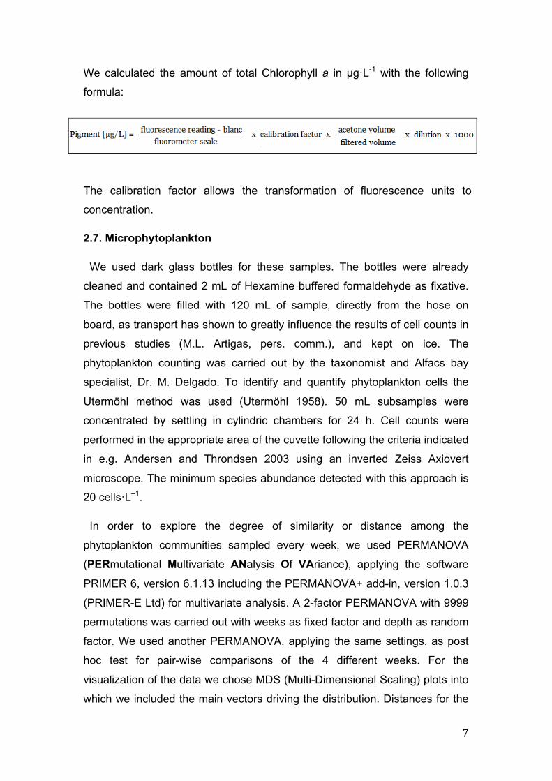
The PERMANOVA analysis showed that the variability of the phytoplankton
distribution was highly influenced by time (i.e. the sampled week) and depth
(p<0.0001 and p=0.0092, respectively). When exploring the particular
influence of the sampled depths, as the 6 categories for depth resulted in a
loss of 5 degrees of freedom further analysis did not give additional
information due to lack of statistical power. However, the MDS graph (Fig. 7)
revealed that samples from, 4.5 and 5.5 m were grouped somehow apart
(towards the center) from the rest of the samples (towards the periphery). The
pair-wise test revealed that each week significantly differed from the others
(Table 2). The main vectors for week 1 were Protoperidinium diabolus and P.
oblongum, Pseudo-nitzschia spp. (potentially Amnesic Shellfish Poisoning –
ASP- producer) and small dinoflagellate cysts; for week 2, small, unidentified
dinoflagellates and for week 3, heterotrophic Gyrodinium spp. and
Gymnodinium elongatum. Week 4 was characterised by coccolithophorids
smaller than 10 µm and Pseudo-nitzschia sp.1. Using Utermöhl, it was not
possible to identify Pseudo-nitzschia to species level, yet this species could
clearly be distinguished from the whole Pseudo-nitzschia spp. group.
Fig. 7. MDS plot showing the Canberra metric dissimilarities between samples; labels refer to depth of sample. Vector’s represent variables with most influence on sample distribution. Vector length represents influence of taxons to dissimilarity.

19
Table 2. p-Values for pair-wise PERMANOVA.
Regarding the potentially harmful phytoplankton species, the following taxa
were seen along our studied period. The dinoflagellates Alexandrium
minutum, several species of Dinophysis, Gonyaulax polygramma, Gonyaulax
spp., Gymnodinium sanguineum, Karlodinium spp., Lingulodinium polyedrum
and Protoceratium reticulatum. And the diatom Pseudo-nitzschia spp. Barring
Karlodinium spp. and Pseudo-nitzschia spp., all of the observed harmful
species presented low concentration values (between 20 and 600 cells·L-1).
Pseudo-nitzschia spp. decreased from more than 50000 cells·L-1 in the 2nd
week to a mean value of 300 cells·L-1 in the last week. And finally Karlodinium
spp. presented a maximum concentration of 77000 cells·L-1 in week 1, but this
specie is not toxic below 100000 cells·L-1. Thus, regarding these results, we
did not take into account anymore for this study.
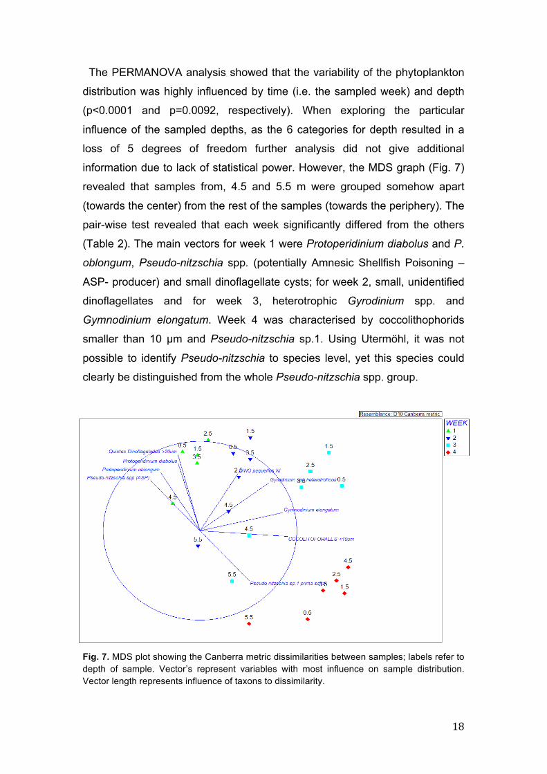
3.4. Nanophytoplankton and Cyanobacteria
Among the nanophytoplankton, NFs showed the highest abundances. ANF
smaller than 5 µm were the most abundant group during the four weeks in all
6 depths. They followed a similar pattern over depth in all weeks, with the
minimum concentration at surface and the maximum at or below the
chlorophyll maximum. These concentration maxima for each week were,
respectively: 1.1x10⁷ cells·L-1 at 5.5 m, 6.9x10⁶ cells·L-1 at 3.5 m, 1.6x10⁷
cells·L-1 at 4.5 m and 9.6x10⁶ cells·L-1 at 4.5 m. The NFs bigger than 5 µm,
both auto- and heterotrophic, appeared in lower abundances: HNF with
concentrations between 4.2 x 10⁴ cells·L-1 - 2.5 x 10⁵ cells·L-1 and ANF
20
between 1.2 x 10⁵ cells·L-1 and 1.1 x 10⁶ cells·L-1. They did not follow a clear
pattern over depth.
Fig. 8. Abundance and distribution of nanoflagellates (ANF and HNF bigger and smaller than 5µm) along the water column. A, B, C and D refer to week 1, 2, 3 and 4 respectively.
4. DISCUSSION
Our results showed a variable physical dynamic . The mixed water column in
weeks 1 and 4 was probably caused by strong wind events. In weeks 1 and 4,
strong Mestral and Garbí, wind events, respectively, probably caused the
mixing of the water column. As there was no significant rain event in any of
those weeks, the salinity differences were mainly due to freshwater inputs
from the northern edge caused by rice cultivation. These findings are in
accordance with the findings of e.g. Camp (1994) and Solé et al (2009). We
expected that turbidity could match somehow the observed mixing-
21
stratification patterns. Turbidity is caused by the different particles suspended
in the water column, including phytoplankton and particles from fresh-water
run-off of the rice fields, which, close to the shore, drain directly into the bay.
We would have expected turbidity to be higher in the weeks with a mixed
water column than in the weeks with stratification, because the shallow water
column should favor mixing with the muddy bottom of the bay. However, the
maximum turbidity values for weeks 1 and 4 were, approximately, the
minimum ones for weeks 2 and 3. It might be that there was more “clear”
Mediterranean water coming into the bay and/or that biological filtration was
enhanced. The main filter feeders in the bay are the cultivated mussels, but in
those weeks a Mnemiopsis leidyi bloom was observed (Neszi, personal
communication), an invasive ctenophora that has supposedly established its’
whole live cycle in the bay (Fuentes, Angel et al. 2010).
Nutrient concentrations were low and consumed during the studied period,
except for silicate, which increased. Somehow, the values were even lower
than expected. This could be the result of the consumption by phytoplankton
in the previous weeks of our samplings. This hypothesis will be considered
within the ECOALFACS project, as it covered a more extensive sampling
period (March to July). Regarding the particular elements, previous
investigations (Krom et al. 1991; Estrada et al. 1993) point to phosphorous as
the main limiting nutrient in the NW Mediterranean, demonstrating that the
decline of the late winter bloom is caused by the depletion of dissolved
inorganic nutrient, particularly phosphorous (Duarte unpublished in Mura et al.
1996). Indeed, the Redfield ratio (Redfield 1934) in our samples N:P>>16
(not shown) corroborates this limiting role of phosphorous in Alfacs bay as
also suggested by previous studies (Vidal 1994). P seems to be present also
in low concentrations in the fresh water of the discharge channels (Artigas et
al. submitted), indicating that it can also be retained on the rice fields (Llebot
et al. 2010).
Interestingly, silicate accumulated from week 1 to 4. This trend could be
related to the lack of silicate consumption by diatoms that decayed
concurrently during this period (Annex Fig. 7). The decay of diatoms can be in
part due to an overcompetition by nanoflagellates, as they are in high

22
abundances. Those organisms could uptake ammonium, a component that
indicates nutrient regeneration within both, the planktonic and the benthonic
microbial communities (Vidal et al. 1992).
The lack of increase in the chlorophyll concentration over time is coherent
with the low nutrient concentrations discussed above. The fact that most part
of the chlorophyll was contributed by phototrophic organisms smaller than 10
µm is consistent with a likely utilization of recycled nutrients as well. It can be
also noted that the partitioning of chlorophyll agrees well with the
phytoplankton counts obtained by the two used methods, i.e. Utermöhl (1958)
and DAPI (Kapuscinski 1995) methods (Fig. 5).
The observed succession of the phytoplankton community (Fig. 6) could be
the following. Our period of study would start with a diverse community, in
which coccolithophorids are at almost undetectable limits, but dinoflagellates,
diatoms and nanoflagellates coexist. In the second week, while dinoflagellates
start to decrease, it can be seen a peak on the diatom's community. We could
speculate that this increase was driven by the observed peak of silicate in that
week at the same depth (Fig. 4). Towards week 3, diatoms decreased notably
suggesting the end of what could have been their spring bloom, which is
consistent with the observed increase in silicate's concentration (Fig. 4), as it
is not being consumed . Contemporaneously, coccolithophorids proliferated,
agreeing with Margalef's Mandala (Annex, fig.1), in which the succession for
these groups would be: diatoms, coccolithophorids and dinoflagellates, as this
last group proliferated again in the last week. The high concentration of NFs in
the 3rd week at 4.5 m coincided with a little peak of ammonium, suggesting
that they could be proliferating from recicled nutrients. It could be
hypothesized that the growth of dinoflagellates in the last week could be given
by the high abundance of NFs the week before, although we could not discard
that they could be different water bodies. Taking all of this into account, the
succession of the future will depend on the diatom's competitive capacity
versus the NFs, since if these ones uptake the P, the diatoms will not be able
to proliferate even with high concentration of silicate. So they would have to
wait until NFs' predator outcompete them (such as dinoflagellates or high
abundances of HNFs)

23
Our MDS plot corroborates the different succession of groups along the 4
weeks. The plot suggests cysts of dinoflagellates, Protoperidinium oblongum,
Protoperidinium diabolus, Pseudo-nitzschia spp., Pseudo-nitzschia sp1 and
cocolitophorids smaller than 10 µm to be the main drivers for the differences
in between the weeks. This is probably related to the dynamics of the water
column: the weeks more influenced by the presence of the diatom Pseudo-
nitzschia are the first and the fourth ones, agreeing with a mixed water
column. According to the conceptual model of Margalef's Mandala (1978)
(Annex, Fig. 1), high turbulence favors diatoms' proliferation as this motion
avoids their sinking. Our analysis suggests that week 1 was also influenced
by the presence of the dinoflagellate Protoperidinium. Since we don't have
data for what happened before, we assume that this was due to the transition
between a stratified to a mixed water column. Dinoflagellates are known to be
favoured in a stratified water column, as the presence of flagella gives them
the capacity of movement and hence the power to follow light and nutrient
gradients relevant to their growth (Estrada and Berdalet 1997).
Significant differences in between depth could be observed when used as a
random factor in the overall PERMANOVA. Nevertheless, it is far fetched to
state that differences in depth are truly significant, due to the lack of statistical
power of our analysis. Regardless, our MDS plot indicates that the samples of
4.5 m and 5.5 m are separated from the samples above, especially in the
stratified weeks. It seems logical that the weeks with the mixed water column
did not show those differences as clearly as the stratified weeks did. The
bottom layers were characterized by the presence of benthic microalgae,
mainly diatoms, from the resuspended sediments. In weeks 2 and 3 the
pycnocline was located around 4 m depth, as revealed in previous studies
(e.g. Camp & Delgado 1987; Artigas et al. submitted). As expected, the
organisms that marked that distribution along depth were the dinoflagellates,
most likely favored under calm water conditions because their ability to swim.
It is important to note however that, Alfacs bay, even during mixing periods
the turbulent kinetic energy dissipation rates were low and compatible with the
swimming speeds of dinoflagellates (Artigas and Berdalet, pers. comm.). Due
to the low number of replicates, and since our data are not normally

24
distributed, a Principal Component Analysis (PCA) approach, which is often
used to evaluate phytoplankton data (f. e. Llebot et al. 2011), was impossible.
We are aware that our four weeks of study are not independent samples, as
they are continuous in time; neither are our depths independent from each
other in space. Yet, our analysis provides an important insight to the
phytoplankton dynamics in the bay: high short-term temporal and spatial
variability of the phytoplankton community in the bay, as also noted elsewhere
(e.g. Artigas et al. submitted).
A really interesting trend could be observed in our graphical analysis: a clear
trophic relationship between ANFs and HNFs (Fig.8). It can be perfectly seen
the trend they both follow: HNFs, always in lower abundances, show the
same variability pattern over depth as the ANFs, they preys. This is the first
study documenting the spatio-temporal changes in the abundances of these
organisms. New questions can now be formulated regarding their importance
in the microbial web structure and dynamics in Alfacs Bay. This is already an
undergoing research in our group.
5. CONCLUSIONS
- The water column presented a high short-term variability given by physical
drivers (such as wind events, radiation, freshwater discharges). It started well-
mixed the first week, stratified in weeks 2 and 3 and mixed again in week 4.
- Really low chlorophyll a amounts were observed, suggesting a limitation
driven by nutrients. This was supported by the low and decreasing nutrients'
concentrations from week 1 to week 4, except for silicate, which increased
towards the last week due to the lack of consumption by diatoms.
- The observed phytoplankton succession was given by turbulence and
nutrient availability (agreeing with Margalef's Mandala) and also by
competition between groups. The whole four weeks were notably dominated
by nanoflagellates. These small organisms coexisted with diatoms and
dinoflagellates the first half of the studied period, but as nutrient went
25
decreasing and the flagellates went increasing, they outcompeted the other
organisms.
- There was an evident trophic relationship between heterotrophic (predator)
and autotrophic (prey) nanoflagellates.
- Several potentially harmful species were detected, but since they were at
really low concentrations, they were not taken into account.

26
6. REFERENCES
Andersen, P. and J. Throndsen (2003). "Estimating cell numbers."
Monographs on Oceanographic Methodology11.
Artigas, M. L., C. Llebot, O. N. Ross, N. Z. Neszi, V. Rodellas, J. Garcia-Orellana, P. Masqué, J. Piera, M. Estrada, E. Berdalet. "Understanding the spatio-temporal variability of phytoplankton biomass distribution in a microtidal estuary: is Alfacs Bay a phytoplankton bloom incubator?" Submitted to Deep-Sea Res. Part II, Topics in Oceanography.
Berdalet, E. and M. Estrada (1997). "Phytoplankton in a turbulent world." Scientia Marina61: 125-140. Camp, J. (1994). "Aproximaciones a la dinámica ecológica de una bahía estuárica mediterránea." Barcelona, Spain: University of Barcelona. Doctoral thesis. Camp, J. and M. Delgado (1987). "Hidrografía de las bahías del delta del Ebro." Investigaciones Pesqueras51: 351-369.
Camp, J., J. Romero, et al. (1992). "Production-consumption budget in an estuarine bay: how anoxia is prevented in a forced system." Homage to Ramon Margalef, or, Why there is such pleasure in studying nature8: 145-152. Colomé, J. V. F., J. Camp, et al. (1997). "Los medios acuáticos del delta del ebro y su capacidad de producción." Revista de obras públicas 3368: 67-71.
Crumpton, W. (1987). "A simple and reliable method for making permanent mounts of phytoplankton for light and fluorescence microscopy." Limnology and Oceanography: 1154-1159. Estrada, M., C. Marrase, et al. (1993). "Variability of deep chlorophyll maximum characteristics in the Northwestern Mediterranean." Marine ecology-progress series92: 289-289.
Fuentes, V. L., D. L. Angel, et al. (2010). "Blooms of the invasive ctenophore, Mnemiopsis leidyi, span the Mediterranean Sea in 2009." Hydrobiologia 645(1): 23-37.
Garcés, E., M. Delgado, et al. (1999). "In situ growth rate and distribution of the ichthyotoxic dinoflagellate Gyrodinium corsicum Paulmier in an estuarine embayment(Alfacs Bay, NW Mediterranean Sea)." Journal of Plankton Research21(10): 1977-1991.

27
GEOHAB, 2001. Global Ecology and Oceanography of Harmful Algal Blooms, Science Plan. P. Glibert and G. Pitcher (eds). SCOR and IOC, Baltimore and Paris. 87 pp.
Kapuscinski, J. (1995). "DAPI: a DNA-Specific Fluorescent Probe." Biotechnic & Histochemistry70(5): 220-233.
Konrad, M., T. Pamminger, et al. (2012). "Two pathways ensuring social harmony." Naturwissenschaften: 1-10.
Lalli, C. M. and T. R. Parsons (1997). Biological oceanography: an introduction, Butterworth-Heinemann. Chapter 3. Llebot, C., J. Solé, et al. (2011). "Hydrographical forcing and phytoplankton variability in two semi-enclosed estuarine bays." Journal of Marine Systems86: 69-86.
Llebot, C., Y. H. Spitz, et al. (2010). "The role of inorganic nutrients and dissolved organic phosphorus in the phytoplankton dynamics of a Mediterranean bay:: A modeling study." Journal of Marine Systems83(3-4): 192-209. Margalef, R. (1978). "Life-forms of phytoplankton as survival alternatives in an unstable environment." Oceanologica acta1(4).
Margalef, R. (1980). La biosfera: entre la termodinámica y el juego. Ed. Omega, Barcelona. 236 pp. Parsons T, Maita Y, Lalli C (1984) "A manual of chemical and biological methods for sea water analysis". Pergamon Press, Oxford Redfield, A. C. (1934). "On the proportions of organic derivatives in sea water and their relation to the composition of plankton." James Johnstone memorial volume176: 92.
Safi, K. A. and J. A. Hall (1997). "Factors influencing autotrophic and heterotrophic nanoflagellate abundance in five water masses surrounding New Zealand." New Zealand journal of marine and freshwater research31(1): 51-60. Solé, J., A. Turiel, et al. (2009). "Climatic forcing on hydrography of a Mediterranean bay (Alfacs Bay)." Continental Shelf Research29(15): 1786-1800.

28
Utermöhl, H. (1958). "Zur vervollkommnung der quantitativen phytoplankton-methodik." Mitt. int. Ver. theor. angew. Limnol.9: 1-38.
Vidal, M., J.-A. Morguí, et al. (1997). "Factors controlling seasonal variability of benthic ammonium release and oxygen uptake in Alfacs Bay (Ebro Delta, NW Mediterranean)." Hydrobiologia350(1): 169-178. Vidal, M., V. Morguí, et al. (1992). "Factors controlling spatial variability in ammonium release within an estuarine bay (Alfacs Bay, Ebro Delta, NW Mediterranean)." Hydrobiologia235(1): 519-525.
Vidal, M., J. Romero Sánchez, et al. (1989). "Sediment-water nutrient fluxes: Preliminary results of in situ measurements in Alfaques Bay, Ebro River Delta." Vila, M., J. Camp, et al. (2001). "High resolution spatio-temporal detection of potentially harmful dinoflagellates in confined waters of the NW Mediterranean." Journal of Plankton Research23(5): 497-514.
Vila, M. and M. Masó (2005). "Phytoplankton functional groups and harmful algae species in anthropogenically impacted waters of the NW Mediterranean Sea." Scientia Marina69(1): 31-45.

1
ANNEX This section includes images and some data that complement the study presented here.
Fig. A. Modified Margalef's mandala (Margalef, 1978). Graphic representation of the major phytoplankton life forms in an ecological space defined by nutrient concentration and turbulence.
Fig. B. SAIV A/S SD204 STD, used in ECOALFACS project’s cruises. Photo: Laia Viure.

2
Fig. C. Swinnex system used for filtering the samples for chlorophyll analysis.
Fig. D. Turner Designs Fluorometer used for the estimation of chlorophyll a.
Fig. E. Turner Designs Fluorometer's scale.

3
Fig. F. Vertical profiles for temperature, salinity and turbidity for each week. Data given by the CTD casts.

4
Fig. G. Vertical
variability of diatoms' abundance
and distribution along the studied
period.