relationship between hypocentral distributions and vp/vs ... · relationship between hypocentral...

Title

Relationship between hypocentral distributions and Vp/Vs ratiostructures inferred from dense seismic array data: a case studyof the 1984 western Nagano Prefecture earthquake, centralJapan

Author(s) Doi, I.; Noda, S.; Iio, Y.; Horiuchi, S.; Sekiguchi, S.

Citation Geophysical Journal International (2013), 195(2): 1323-1336

Issue Date 2013-10-08

URL http://hdl.handle.net/2433/179457

Right © The Authors 2013. Published by Oxford University Press onbehalf of The Royal Astronomical Society.

Type Journal Article

Textversion publisher

Kyoto University

Geophysical Journal InternationalGeophys. J. Int. (2013) 195, 1323–1336 doi: 10.1093/gji/ggt312Advance Access publication 2013 August 30

GJI

Sei

smol

ogy

Relationship between hypocentral distributions and Vp/Vs ratiostructures inferred from dense seismic array data: a case study of the1984 western Nagano Prefecture earthquake, central Japan

Issei Doi,1 Shunta Noda,2 Yoshihisa Iio,1 Shigeki Horiuchi3 and Shoji Sekiguchi41Disaster Prevention Research Institute, Kyoto University, Gokasho, Uji, Kyoto 611-0011, Japan. E-mail: [email protected] Technical Research Institute, 2-8-38 Hikari-cho, Kokubunji-shi, Tokyo 185-8540, Japan3Home Seismometer Corporation, 67-1 Kamisakai, Tsukuba, Ibaraki 305-0011, Japan4National Research Institute for Earth Science and Disaster Prevention, 3-1, Tennodai, Tsukuba, Ibaraki 305-0006, Japan

Accepted 2013 August 1. Received 2013 July 29; in original form 2013 February 26

S U M M A R YWe conducted a three-dimensional traveltime tomographic reconstruction in and around thesource region of the 1984 western Nagano Prefecture earthquake to investigate the generationprocess for the main shock and associated swarm activity. Up to 220 000 high-resolution trav-eltime records (2 ms error) were compiled from a dense seismic network. From these records,we performed accurate, high-resolution calculations to estimate hypocentre distributions andthree-dimensional velocity structure. Most hypocentres aligned along the same path or withinthe same plane, rather than in three-dimensional clusters. Hypocentres in the swarm regionare located in regions with low Vp/Vs ratios, while few earthquakes occurred in regions withhigh or normal Vp/Vs ratios. We suggest that differences in the number of small fractures andfluid content between these two regions influenced the seismic activity. Rupture propagationassociated with the main shock appears to be confined by relatively higher Vp/Vs surroundings,and a low-velocity region which limits its vertical extent.

Key words: Seismic tomography; Fractures and faults; Crustal structure.

1 I N T RO D U C T I O N

Elucidating generation processes of earthquakes is critical for long-term forecasting and preparedness. At present, however, we do notfully understand how earthquakes—especially crustal earthquakes,are generated. Recently, studies have posited that the generationmechanism of crustal earthquakes relates to fluids in the crust. Iioet al. (2002) suggested that water issuing upwards from subduct-ing slabs drives crustal earthquakes. Vidale & Shearer (2006) andYukutake et al. (2011) also found that fluid diffusion may causeswarm migration.

In studies of heterogeneous structures within the source regionsof large earthquakes, low-velocity regions have been found adjacentto the hypocentre. Studies of waves trapped within fault zones foundthat fractures serve to lower wave velocity in the vicinity of the faultzone (Li et al. 1994; Mizuno et al. 2004). Using extremely high-density aftershock observations, Okada et al. (2006) determinedthat parts of the 2004 Chuetsu earthquake faults were located inlow-velocity regions. Hasegawa et al. (2009) reported that low-velocity regions have been detected just beneath the main shockfaults of many crustal earthquakes. Moreover, Tian et al. (2007)suggest that the existence of fluids weakens the rocks around thefaults of crustal earthquakes to trigger large events in California.These studies suggest that fluids beneath the main shock hypocentre

migrate into the fault zone and increase the pore pressure to generatethe main shock. How fluids interact with subsurface structures, andhow these interactions relate to earthquake generation, however, arenot fully understood.

In order to investigate the earthquake generation processes, Iioet al. (1999) installed a high-density seismic network in and aroundthe source region of the 1984 Nagano Prefecture earthquake. Datafrom this network enable us to more precisely estimate hypocentrelocations and velocity structures. These parameters can, in turn,reveal the behaviour of crustal fluids. In this study, we estimatesubsurface three-dimensional velocity structure at ∼1.5 km reso-lution and interpret relationships among hypocentre distributionsand low-velocity anomalies to elucidate generation processes forearthquakes.

2 G E O P H Y S I C A L S E T T I N G O F T H E 1 9 8 4W E S T E R N NA G A N O P R E F E C T U R EE A RT H Q UA K E

The 1984 western Nagano Prefecture earthquake had a Japan Metro-logical Agency (JMA) magnitude (Mj) of 6.8 and occurred onSeptember 14 about 10 km southeast of Mt. Ontake, an active vol-cano in central Japan (Fig. 1). The earthquake caused extensive

C© The Authors 2013. Published by Oxford University Press on behalf of The Royal Astronomical Society. 1323

at Kyoto U

niversity Library on N

ovember 14, 2013

http://gji.oxfordjournals.org/D

ownloaded from

http://gji.oxfordjournals.org/


1324 I. Doi et al.

Figure 1. Map showing the area analysed in this study. A large open star and a dashed rectangle mark the main shock epicentre and fault plane (respectively)of the 1984 western Nagano Prefecture earthquake, as estimated by Yoshida & Koketsu (1990). The open rectangle shows the analysis area of this study. Redtriangles and solid lines denote Quaternary volcanoes and active faults (Research Group for Active Faults of Japan 1991), respectively. Gray dots indicateepicentres of earthquakes which occurred from 1997 to 2005 at depths of less than 10 km, as entered in the JMA catalog. A gray dashed ellipse denotes theswarm source region before the main shock. Two black small stars represent large aftershocks. A dashed ellipse shows the uplift region estimated by Kimataet al. (2004). The blue inverted triangle shows a hydrothermal feature with elevated δ13C values for CO2 (Takahata et al. 2003).

damage and induced landslides. The earthquake’s fault was inter-preted by Yoshida & Koketsu (1990) as a right lateral, ENE-WSWtrending one.

Ooida et al. (1989) investigated the seismicity around thehypocentral region before the main shock occurrence. High seis-mic activity in the hypocentral region of this earthquake started inMay 1978, 1 yr before the eruption of Mt. Ontake. They pointedout that the hypocentral region experienced swarm-type seismicityuntil this main shock. This swarm activity (denoted by gray-dashedellipse in Fig .1) first started south of the main shock hypocentreand extended north of it. After the main shock, aftershocks withstrike-slip focal mechanisms occurred along the main shock fault.Aftershock activity on the main shock fault was low but M 6.2and M 5.3 events occurred 10 km western and eastern side of thefault within 20 d, respectively (shown by small stars in Fig. 1).

Swarm activity also continued mainly in the northeastern region ofthe main shock fault and elevated seismic activity continues to thepresent time with events larger than Mj ∼ 4.0 occurring about every2 yr. Fig. 1 shows epicentral distributions from 1997 to 2005 forevents shallower than 10 km as listed in the JMA catalog. Seismicactivity occurs not only along the main shock fault plane, but also asswarm-like activity in the eastern parts of the source region (Fig. 1).Most of the hypocentres are concentrated in the shallow subsurfaceat depths of 2–6 km.

Many studies have investigated the structures and mechanismsrelated to volcanic activity and earthquake generation in this region.Tanaka & Ito (2002) estimated a relatively high crustal heat flow of70–220 mW m−2 for the region and suggested that it confines thedepth of hypocentres to the shallow subsurface. Kasaya & Oshiman(2004) and Yoshimura et al. (2011) modelled a low-resistivity

at Kyoto U


ovember 14, 2013


ownloaded from



Relationship between hypocentres and velocity structure 1325

region near the main shock hypocentre and swarm region. Taka-hata et al. (2003) detected an anomalous temporal increase during1996–2000 in δ13C values of CO2 from a hydrothermal feature lo-cated directly above the swarm, as indicated by the blue invertedtriangle in Fig. 1. This study concluded that the enriched fluidsoriginated from the mantle. From levelling observations, Kimataet al. (2004) found that 3–6 mm of uplift occurred in the regionabove the swarm (indicated by a dashed ellipse in Fig. 1) from 2002to 2004. These workers interpreted the observations according tomodels showing fluid plumes rising from depths of 1–2 km. Thesestudies also suggest that fluids from the mantle are rising to a depthof about 2 km in and around the main shock source region.

In this region, Hirahara et al. (1992) employed approximately7000 traveltimes from the 1986 Joint University aftershock obser-vation data set and conducted the traveltime tomography to estimatevelocity structure with the spatial resolution of 2 km. They foundthat the low-velocity regions were located in the large amount ofdislocation and the retarded rupture front of the main shock fault.

3 D E N S E A R R AY DATA

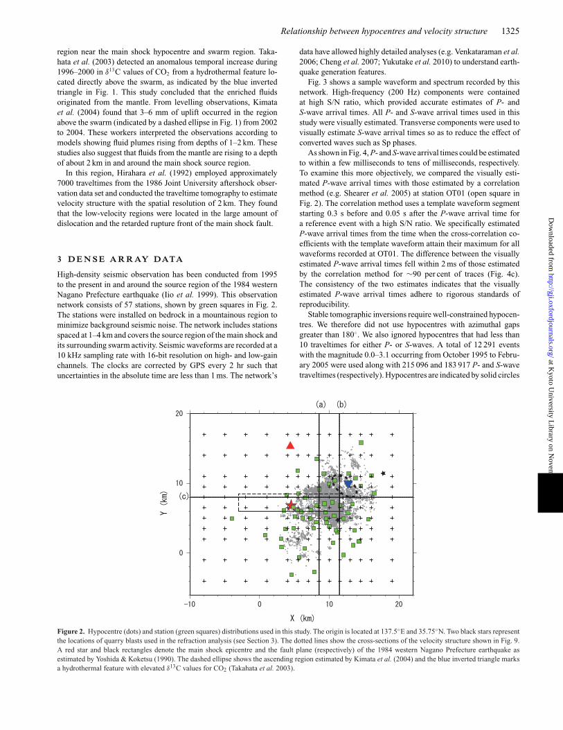
High-density seismic observation has been conducted from 1995to the present in and around the source region of the 1984 westernNagano Prefecture earthquake (Iio et al. 1999). This observationnetwork consists of 57 stations, shown by green squares in Fig. 2.The stations were installed on bedrock in a mountainous region tominimize background seismic noise. The network includes stationsspaced at 1–4 km and covers the source region of the main shock andits surrounding swarm activity. Seismic waveforms are recorded at a10 kHz sampling rate with 16-bit resolution on high- and low-gainchannels. The clocks are corrected by GPS every 2 hr such thatuncertainties in the absolute time are less than 1 ms. The network’s

data have allowed highly detailed analyses (e.g. Venkataraman et al.2006; Cheng et al. 2007; Yukutake et al. 2010) to understand earth-quake generation features.

Fig. 3 shows a sample waveform and spectrum recorded by thisnetwork. High-frequency (200 Hz) components were containedat high S/N ratio, which provided accurate estimates of P- andS-wave arrival times. All P- and S-wave arrival times used in thisstudy were visually estimated. Transverse components were used tovisually estimate S-wave arrival times so as to reduce the effect ofconverted waves such as Sp phases.

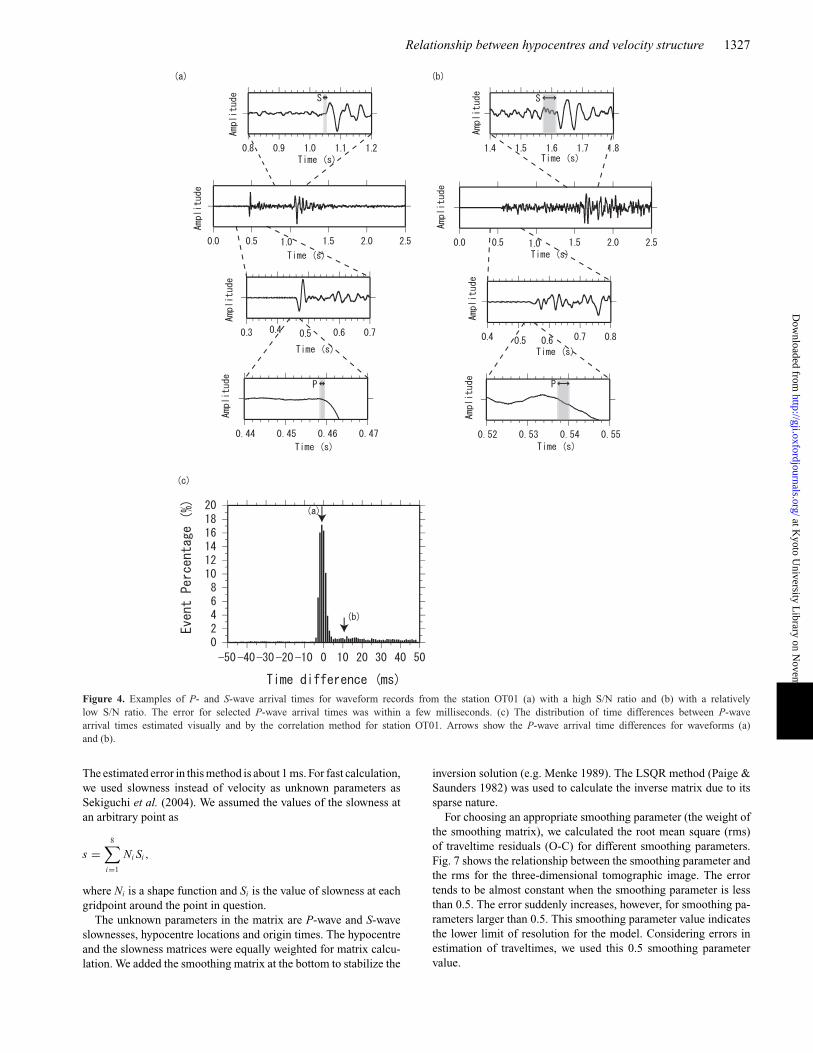
As shown in Fig. 4, P- and S-wave arrival times could be estimatedto within a few milliseconds to tens of milliseconds, respectively.To examine this more objectively, we compared the visually esti-mated P-wave arrival times with those estimated by a correlationmethod (e.g. Shearer et al. 2005) at station OT01 (open square inFig. 2). The correlation method uses a template waveform segmentstarting 0.3 s before and 0.05 s after the P-wave arrival time fora reference event with a high S/N ratio. We specifically estimatedP-wave arrival times from the time when the cross-correlation co-efficients with the template waveform attain their maximum for allwaveforms recorded at OT01. The difference between the visuallyestimated P-wave arrival times fell within 2 ms of those estimatedby the correlation method for ∼90 per cent of traces (Fig. 4c).The consistency of the two estimates indicates that the visuallyestimated P-wave arrival times adhere to rigorous standards ofreproducibility.

Stable tomographic inversions require well-constrained hypocen-tres. We therefore did not use hypocentres with azimuthal gapsgreater than 180◦. We also ignored hypocentres that had less than10 traveltimes for either P- or S-waves. A total of 12 291 eventswith the magnitude 0.0–3.1 occurring from October 1995 to Febru-ary 2005 were used along with 215 096 and 183 917 P- and S-wavetraveltimes (respectively). Hypocentres are indicated by solid circles

Figure 2. Hypocentre (dots) and station (green squares) distributions used in this study. The origin is located at 137.5◦E and 35.75◦N. Two black stars representthe locations of quarry blasts used in the refraction analysis (see Section 3). The dotted lines show the cross-sections of the velocity structure shown in Fig. 9.A red star and black rectangles denote the main shock epicentre and the fault plane (respectively) of the 1984 western Nagano Prefecture earthquake asestimated by Yoshida & Koketsu (1990). The dashed ellipse shows the ascending region estimated by Kimata et al. (2004) and the blue inverted triangle marksa hydrothermal feature with elevated δ13C values for CO2 (Takahata et al. 2003).

at Kyoto U


ovember 14, 2013


ownloaded from



1326 I. Doi et al.

Figure 3. An example of a waveform and spectra observed from the network used in this study (Iio et al. 1999). The magnitude of the event was 0.7. Timewindows for the pre-signal and P-wave arrival shown in the upper panel were used to estimate spectra in the lower panel.

in Fig. 2. The hypocentre locations and velocity structures would beavailable at greater precision than that used in previous studies (e.g.Hirahara et al. 1992) due to the large amount of high-quality datafor traveltime tomography in this region. Our data set also has a lotof events in the swarm region, which expects us to obtain detailedvelocity structures around there.

4 M E T H O D S

We set the X, Y and Z axes as the strike direction of the mainshock fault (N70◦E; as estimated in Yoshida & Koketsu 1990),the perpendicular direction and the depth directions, respectively(Fig. 2). The area analysed spanned 32, 26 and 12 km in the X,Y and Z directions, respectively, and included the source regionof the main shock and the swarm activity. Figs 2 and 5 show thelateral and vertical grid locations (respectively) used for the three-dimensional inversion. Given errors in the estimated arrival times,horizontal grids were overlaid at 1.5 km intervals in the central partof the analysis area, where many of the hypocentres used in theanalysis were located. The grid spacing was 3 km in surroundingareas. Vertical grids were overlaid at 1 km intervals for depths of lessthan 4 km, and at 2 km intervals for depths greater than 4 km. We setgrid’s height to 3 km in order to take the station height into account,given that the regolith extends to about this height. The slownessvalues, which we used in the calculation instead of velocity, wereinterpolated by shape functions for an arbitrary point within eachgrid.

Tomographic inversion was performed using a three-step method.First, we determined the initial hypocentre locations and origintimes assuming a fixed initial velocity structure. Next, we estimatedthe one-dimensional velocity profile and recalculated hypocentresand station corrections using a one-dimensional inversion. Lastly,we constructed a tomographic image to obtain three-dimensionalvelocity perturbations together with recalculated hypocentres andstation corrections. This procedure yields more precise hypocentrelocations and velocity structure than those based on initial hypocen-tre locations and the initial one-dimensional velocity structure (e.g.Shibutani et al. 2005). We iterated each step three times to obtainthe final model.

The initial one-dimensional P-wave velocity structure (shownin Fig. 5) was one-dimensional traveltime tomographic modelby Hirahara et al. (1992). The network used in this study alsorecorded seismic charges and quarry blasts (denoted by blackstars in Fig. 2). Fig. 6 shows the observed, reduced P-wave trav-eltimes from the quarry blasts according to the known epicen-tral distances, with the theoretical traveltime curve calculatedaccording to the initial one-dimensional velocity structure. Thecorrespondence between the theoretical and observed traveltimesdemonstrates the consistency of the initial velocity structure. Theinitial S-wave velocity model was set by dividing P-wave oneby 1.73.

We used a pseudobending method to perform ray calculation(Um & Thurber 1987), where the initial path is divided into severalsmall segments and changed by a geometric interpretation of theray equations so that the traveltime along this path is minimized.

at Kyoto U


ovember 14, 2013


ownloaded from




Figure 4. Examples of P- and S-wave arrival times for waveform records from the station OT01 (a) with a high S/N ratio and (b) with a relativelylow S/N ratio. The error for selected P-wave arrival times was within a few milliseconds. (c) The distribution of time differences between P-wavearrival times estimated visually and by the correlation method for station OT01. Arrows show the P-wave arrival time differences for waveforms (a)and (b).

The estimated error in this method is about 1 ms. For fast calculation,we used slowness instead of velocity as unknown parameters asSekiguchi et al. (2004). We assumed the values of the slowness atan arbitrary point as

s =8∑

i=1

Ni Si ,

where Ni is a shape function and Si is the value of slowness at eachgridpoint around the point in question.

The unknown parameters in the matrix are P-wave and S-waveslownesses, hypocentre locations and origin times. The hypocentreand the slowness matrices were equally weighted for matrix calcu-lation. We added the smoothing matrix at the bottom to stabilize the

inversion solution (e.g. Menke 1989). The LSQR method (Paige &Saunders 1982) was used to calculate the inverse matrix due to itssparse nature.

For choosing an appropriate smoothing parameter (the weight ofthe smoothing matrix), we calculated the root mean square (rms)of traveltime residuals (O-C) for different smoothing parameters.Fig. 7 shows the relationship between the smoothing parameter andthe rms for the three-dimensional tomographic image. The errortends to be almost constant when the smoothing parameter is lessthan 0.5. The error suddenly increases, however, for smoothing pa-rameters larger than 0.5. This smoothing parameter value indicatesthe lower limit of resolution for the model. Considering errors inestimation of traveltimes, we used this 0.5 smoothing parametervalue.

at Kyoto U


ovember 14, 2013


ownloaded from



1328 I. Doi et al.

Figure 5. One-dimensional velocity models used as an initial structure in the analysis (solid lines), and obtained from this study (dashed) for (a) P- and(b) S-wave. Closed circles and squares denote grid locations used for the inversion.

Figure 6. Traveltime diagram for quarry blasts shown in Fig. 2. Traveltimes were reduced with the velocity of 5.5 km s−1. The solid line represents thetraveltime curve, which was calculated using the initial velocity structure for the tomographic inversion shown in Fig. 5.

at Kyoto U


ovember 14, 2013


ownloaded from




Figure 7. The relationship between smoothing parameter and rms.

5 R E S U LT S

5.1 Estimated hypocentre locations and velocity structures

Three-dimensional P-wave velocity (Vp) and S-wave velocity (Vs)perturbations from the one-dimensional model in the vertical andhorizontal planes are shown in Figs 8 and 9 (respectively) alongwith Vp/Vs ratios calculated from the magnitudes of Vp and Vs.We masked the regions which are considered not to have sufficientresolutions (for more details, see Section 5.2). A one-dimensionalinversion reduced the rms of O-C for P-wave arrivals after the ini-tial hypocentre determination from 18 to 13 ms. Three-dimensionalinversion further reduced the errors to 9 ms, which totally reducedthe standard deviation by 50 per cent.

5.2 Resolution of the obtained velocity structure

We prepared two kinds of synthetic traveltime data to determine themodel resolution. First, we used a checkerboard procedure (Inoueet al. 1990) to synthesize traveltimes with 5 per cent velocity per-turbations relative to the initial velocity of rays used in the analysis.We estimated the ‘restoration ratios’ which are defined as ratios ofthe obtained velocity perturbations to the given ones. For the seconddata set, we synthesized traveltime data using the final calculatedvelocity model from this study. Random noise (2 ms for P-wavesand 30 ms for S) was introduced to both synthetic traveltime datasets. We inverted the synthetic data in the same manner as that

described in Section 4. We refer to the two velocity models as the‘checkerboard model’ and ‘synthetic model’, respectively.

We show the results of checkerboard model are shown in Figs S1and S2. Fig. 10 shows the final model from tomographic analysis aswell as the synthetic model along the X = 11.5 km cross-section.We drew contour lines in this figure with a restoration ratio of 0.3from the checkerboard model. The restoration ratio was higher than0.3 in the central part of the analysis area at depths shallower than6 km. Comparison of the two models in Fig. 10 shows that thesame velocity perturbations were obtained for regions inside therestoration ratio = 0.3 contour lines. This indicates that the velocityperturbations are well resolved given a restoration ratio greaterthan 0.3.

5.3 Features of hypocentre distribution

Figs 8 and 9 show that most hypocentres are located at depthsof 2–6 km along linear features or planes, and do not fall intothree-dimensional clusters, even in regions with swarm activity.We identified a 5-km-long, near-vertical hypocentre distribution atdepths of 2–6 km near the main shock fault plane, as estimatedby Yoshida & Koketsu (1990; that is, 4 < Y < 6, shown bythe F arrows in Figs 8b and 9a). We also identified alignmentamong hypocentres in the northeastern part of the study regionwhere swarm activity occurs. The most dominant alignments spana distance of 5–10 km, dip 30–60◦ to the northeast and divideinto two parallel planes (shown by arrows S1 and S2 in Figs 9band c).

5.4 Features of the three-dimensional velocity structure

Hypocentres primarily occur in two regions (regions A and B inFigs 8 and 9). Region A, characterized by low Vp, high Vs andvery low Vp/Vs ratios (<1.60), was detected in the swarm regionat depths of 2 km (Figs 8a, 9a and c). Region B, characterized byhigh Vp, high Vs and a slightly low Vp/Vs (1.65–1.70), is locatedat depths greater than 3 km and corresponds to swarm hypocentresS1 and S2 (Figs 8b, 9b and c). A neighbouring feature, region C,is characterized by average to high Vp, average Vs and slightlyelevated Vp/Vs (1.70–1.75), as shown in Figs 8(b), 9(b) and (c).Few earthquakes occur in this region. An additional region withfew hypocentres (region C′) exhibited the same velocity trend asregion C (Figs 8b and 9b). Regions B and C are distributed parallelto the hypocentre alignments S1 and S2. Hypocentre distributionsapparently correlate with Vp/Vs ratios, but not with Vp or Vs. Wealso identified a horizontal, low Vp and low Vs region with highVp/Vs ratios (1.75–1.90) at shallow depths (<2 km). We refer tothis region as region L, as shown in Fig. 9. The schematic figurebased on X = 11.5 cross-section (i.e. the same as Fig. 9b) is shownin Fig. 11.

6 D I S C U S S I O N

6.1 Velocities for the bedrock matrix in the study regionand the nature of velocity changes

The calculated velocity perturbations shown in Figs 8 and 9 arebased on the one-dimensional velocity model. In order to interpretthe heterogeneous subsurface structure in the study region, it is im-portant to consider velocity changes from velocities of rock matrix,which are velocities of rock without fractures. Takeda et al. (1999)

at Kyoto U


ovember 14, 2013


ownloaded from



1330 I. Doi et al.

Figure 8. Horizontal view of P- and S-wave velocity perturbations, and Vp/Vs ratios obtained from the three-dimensional inversion. Black dots denote thehypocentres. The regions with a restoration rate of less than 0.3 were masked.

determined Vp for numerous core samples obtained at depths of331–722 m from five different boreholes located within the studyarea. Their Vp estimations followed methods of Yamamoto et al.(1988, 1991), which estimated Vp for a given rock matrix mate-

rial as the ratio of velocities for saturated versus dry conditions.They found that Vp does not vary by more than 3 per cent fromaverage values regardless of rock type, with the exception of slatesamples (see Table 1). These results suggest that a Vp difference of

at Kyoto U


ovember 14, 2013


ownloaded from




Figure 9. Vertical cross-section of P- and S-wave velocity perturbations along with Vp/Vs ratios obtained from the three-dimensional inversion. Black dotsdenote hypocentres. The regions with a restoration rate of less than 0.3 were masked. The cross-sections for each figure are shown in Fig. 2. The bold line in (a)denotes the fault plane posited by Yoshida & Koketsu (1990). The dashed half ellipse and a blue inverted triangle in (c) show the uplift region (Kimata et al.2004) and the hydrothermal feature with elevated δ13C values for CO2 (Takahata et al. 2003), respectively.

greater than 3 per cent reflects differences in crack density and/orfluid saturation of rocks. Moreover, Vp estimates of Takeda et al.(1999) are 3–5 per cent higher than estimates for depths of lessthan 6 km, as calculated in the one-dimensional model from thisstudy.

Crack densities in the rocks are considered to mainly reflectthe magnitudes of Vs perturbations, regardless of whether theyare saturated or not. Vp/Vs ratios are affected by aspect ra-tios and saturation of cracks. If the aspect ratios are the same,higher Vp/Vs ratios indicate high saturation (Takei 2002). There-fore, the regions with low Vs and high Vp/Vs ratios have lotsof saturated cracks (probably with moderate aspect ratios). Onthe other hand, low Vp/Vs ratios indicate that the cracks are notsaturated.

6.2 Mantle-derived fluids near the surface

Fluids originating from the mantle were detected from a hydrother-mal feature above the low-velocity region L, indicated by the blueinverted triangle in Fig. 9(c) (Takahata et al. 2003). The relativelylow P- and S-wave velocity estimates along with the high Vp/Vsratios in region L suggest a dense volume of cracks saturated withmantle-derived fluids, as described in Section 6.1. This inferenceis supported by JMA catalog entries showing deep, low-frequencyevents recorded at depths of 15–50 km just beneath the study area,which are interpreted as evidence of fluid movement (Ohmi & Obara2002). Surface uplift was also observed in the area marked bythe black, dashed half ellipse in Fig. 9(c) (Kimata et al. 2004).These observations along with other researches suggest that fluids

at Kyoto U


ovember 14, 2013


ownloaded from



1332 I. Doi et al.

Figure 9. (Continued.)

originate in the mantle and ascend through the study area to accu-mulate near the surface.

6.3 The main shock fault plane

We detected a near-vertical hypocentre alignment feature (referredto as ‘F’) near the hypocentre of the 1984 western Nagano Prefectureearthquake. We think that this alignment corresponds to the mainshock fault plane because it shows similar attitudes to those of thefault plane estimated in Yoshida & Koketsu (1990) and the eventshad strike-slip focal mechanisms (Yukutake et al. 2010). The faultplane estimated in this study was located at a distance of 1–2 kmfrom that estimated by Yoshida & Koketsu (1990), as shown inFig. 9(a). This offset is possibly due to the limited coverage of thepermanent JMA network (stations spaced about 50 km apart), asthis was the only network previously available in the study area.We identified the main shock fault from hypocentral distributionsprecisely determined by a seismic network with a much higherstation density.

Surface rupture is an important factor in predicting strong mo-tion and earthquake hazards. No apparent surface rupture occurred

during the 1984 western Nagano Prefecture earthquake (Umedaet al. 1987), in spite of its shallow focal depth and magnitude. Thelow-velocity region L is located at the upper edge of the hypocentrealignment F (Fig. 9a) and the large slip regions of the main shock(Yoshida & Koketsu 1990). These low Vp and Vs regions were at-tributed to saturated cracks described in Section 6.2. Numericalsimulations have shown that fluid-saturated material in the drainagestate decreases the pore pressure along the extensional side to arrestrupture propagation (Viesca et al. 2008; Samuelson et al. 2011).This low-velocity region could have prevented the rupture from ex-tending upwards to the surface (as denoted by a dashed line in theschematic figure, Fig. 11).

Regions C′ is located at the eastern edge of the main shock fault(Fig. 8b), according to the hypocentre distribution of alignmentF. The distributions of Vp/Vs ratios, instead of low velocities asinferred in Hirahara et al. (1992), may be considered to stop therupture propagation.

6.4 Relationship between swarm activity andthe velocity structure

In the swarm activity region, most hypocentres are distributed withintwo regions, regions A and B, which exhibit low to very low Vp/Vsratios. We investigated the relationship between the hypocentral lo-cations and the velocity structure of these regions. Fig. 12 shows his-tograms of earthquake frequencies, grid frequencies and earthquakefrequencies per grid, according to Vp/Vs ratios, for regions with arestoration ratio greater than 0.3. Hypocentre histograms show twolocal peaks corresponding to Vp/Vs ratios of 1.58–1.60 and 1.68–1.70, while grid numbers according to the Vp/Vs ratios are normallydistributed with an average value of around 1.73. This indicatesthat hypocentres are not independent of Vp/Vs ratios. Hypocentrefrequency according to Vp/Vs ratios concentrate at Vp/Vs ratios of1.56–1.60 and 1.68–1.70, which correspond to regions A and B,respectively. Regions C and C′ (with 1.70–1.75 Vp/Vs ratios) haverelatively few earthquakes compared to other areas of the grids.

Assuming a matrix P-wave velocity of 6.24 km s−1 (Takeda et al.1999), the Vp for regions A and B is about 10 and 5 per cent lowerthan the P-wave velocity for the matrix. Assuming a Vp/Vs ratio of1.73 for the bedrock matrix, the Vs for regions A and B is severalpercent lower than the S-wave velocity for the matrix. On the otherhand, in regions C and C′, where few swarm activities are observed,Vp/Vs is normal (around 1.73) and Vs is lower than that in regions Aand B and about 7 per cent lower than the bed rock one. Accordingto the description in Section 6.1, these results indicate that crackdensities are high and they are saturated in regions C and C′, whilethere exist open (or a little saturated) cracks in regions A and B. Theportions of saturated cracks may be responsible for the differencein Vp/Vs ratios. These observations are consistent with the resultsof a three-dimensional electrical resistivity survey that showed lowresistivity in regions C and C′, compared with the surroundingregions (Yoshimura et al. 2011).

Lin & Shearer (2009) and Kato et al. (2010) similarly foundthat regions in swarm source regions have low Vp/Vs ratios. Theseworkers interpreted the anomalies as evidence of cracks with upto several percent saturation. The fact that the hypocentral distri-butions show a linear or a planar trend suggests that the swarmevents occur on the pre-existing fracture systems. Pore pressurelikely increases when the fluids, which are considered to be sup-plied from the mantle, migrate into these open (or a little saturated)cracks, as denoted by red arrows in Fig. 11. This leads to earthquake

at Kyoto U


ovember 14, 2013


ownloaded from




Figure 10. Comparison of the tomographic results from the cross-section shown in Fig. 2 (b). The left panel shows the final tomographic model determinedby this study (same as Fig. 9b). The right panel shows the synthetic model. We show the regions with a restoration ratio greater than 0.3, as calculated from thecheckerboard model.

Figure 11. The schematic figure of the results in this study. Crosses and red arrows denote the earthquake occurrence and fluid flows, respectively. Solid linesdenote the hypocentre distributions, while a dashed line represents that the main shock rupture did not reach the ground surface. The dashed half ellipse anda blue inverted triangle show the uplift region (Kimata et al. 2004) and the hydrothermal feature with elevated δ13C values for CO2 (Takahata et al. 2003),respectively.

at Kyoto U


ovember 14, 2013


ownloaded from



1334 I. Doi et al.

Table 1. P-wave velocities for several bedrock types after Takedaet al. (1999).

Location Depth (m) Rock type P wave velocity (km s−1)

OT-2 331 Dacite 6.24OT-2 448 Porphyrite 6.26OT-2 722 Rhyolite 6.22OT-3 376 Sandstone 6.45OT-3 600 Sandstone 6.27OT-4 705 Slate 5.59OT-5 470 Sandstone 6.17

occurrence (crosses in Fig. 11) in regions A and B. However, if thecracks are saturated as in regions C and C′, pore pressure maynot change so much along with fluid intrusion, resulting in smallnumber of earthquakes.

Many tomographic studies have addressed source regions forlarge inland earthquakes (e.g. Zhao & Negishi 1998; Tian et al.2007; Okada et al. 2008) and swarms (e.g. Vidale & Shearer 2006;Kato et al. 2010; Yukutake et al. 2011). These studies have sug-gested the existence of underlying subsurface fluids and swarmmigration due to their diffusion. Fluid behaviour in the subsurfaceremains poorly understood, however, due to limited informationregarding subsurface structure. Precise modelling reported by thisstudy includes velocity properties of the medium imaged at a resolu-tion of 1.5 km and provides a detailed description of fluid behaviourand its relationship to swarm seismicity. This provides informationfor other study areas where earthquake swarms occur adjacent tovolcanoes.

7 C O N C LU S I O N S

We conducted a three-dimensional traveltime tomography in andaround the source region of the 1984 western Nagano Prefec-ture earthquake (Mj 6.8). We used around 220 000 highly accurateP-wave arrival times (with 2 ms errors) and 180 000 S-wave arrivaltimes (with 20 ms errors) from a dense seismic network (stationspacing 1–4 km) to determine highly accurate hypocentre distribu-tions and detailed three-dimensional velocity structure at depths of2–6 km. Most hypocentres aligned along linear features or planes,rather than in three-dimensional clusters, even in the swarm activityregion. One of the hypocentre alignments coincides with the mainshock fault. Regions with high and normal Vp/Vs ratios, assumed tohave a high and a relatively high density of fluid-saturated cracks,were detected at the upper limit and eastern edge of this hypocentrealignment, respectively. The main shock rupture propagation wasapparently affected by characteristics of the surrounding medium.Hypocentral distributions in the swarm regions correspond to re-gions with low Vp/Vs ratios. The difference between the velocity inthese regions and measured matrix velocities indicates the presenceof unsaturated cracks. Swarm activity occurs when fluids, inferredfrom the distribution of low-velocity regions and from past studiesof the swarm region, migrate into these cracks.

A C K N OW L E D G E M E N T S

We thank Shiro Ohmi for developing the novel data processingsystem used during the first several years of this research effort. Wealso thank Eiji Yamamoto, Hisao Ito, Yasuto Kuwahara and TakaoOhminato for their very helpful contributions regarding borehole

Figure 12. Histograms of estimated hypocentre frequencies, the numbersof the grids and the numbers of the hypocentres per grid, according to Vp/Vsratios for regions with a restoration ratio larger than 0.3, as calculated by thecheckerboard model.

observations. We are grateful to Kaori Takai for her help with dataprocessing. Comments from two anonymous reviewers helped usto improve the manuscript. We used the General Mapping Tool(Wessel & Smith 1991) for drafting the figures presented in thismanuscript. This work was partially supported by JSPS.KAKENHI(19204043), Japan.

at Kyoto U


ovember 14, 2013


ownloaded from




R E F E R E N C E S

Cheng, X., Niu, F., Silver, P.G., Horiuchi, S., Takai, K., Iio, Y. & Ito,H., 2007. Similar microearthquakes observed in western Nagano, Japan,and implications for rupture mechanics, J. geophys. Res., 112, B04306,doi:10.1029/2006JB004416.

Hasegawa, A., Nakajima, J., Uchida, N., Okada, T., Zhao, D., Matsuzawa,T. & Umino, N., 2009. Plate subduction, and generation of earthquakesand magmas in Japan as inferred from seismic observations: an overview,Gondwana Res., 16, 370–400.

Hirahara, K. The Members of the 1986 Joint Seismological Research InWestern Nagano Prefecture, 1992. Three-dimensional P and S wave ve-locity structure in the focal region of the 1984 Western Nagano PrefectureEarthquake, J. Phys. Earth, 40, 343–360.

Iio, Y. et al., 1999. Slow initial phase generated by microearthquakes oc-curring in the Western Nagano Prefecture, Japan. - the source effect,Geophys. Res. Lett., 26, 1969–1972.

Iio, Y., Sagiya, T., Kobayashi, Y. & Shiozaki, I., 2002. Water-weakenedlower crust and its role in the concentrated deformation in the JapaneseIslands, Earth planet. Sci. Lett., 203, 245–253.

Inoue, H., Fukao, Y., Tanabe, K. & Ogata, K., 1990. Whole mantle P-wavetravel time tomography, Phys. Earth planet. Inter., 59, 294–328.

Kasaya, T. & Oshiman, N., 2004. Lateral inhomogeneity deduced from3-D magnetotelluric modeling around the hypocentral area of the 1984Nagano Prefecture earthquake, central Japan, Earth Planets Space, 56,547–552.

Kato, A., Sakai, S., Iidaka, T., Iwasaki, T. & Hirata, N., 2010. Non-volcanicseismic swarms triggered by circulating fluids and pressure fluctuationsabove a solidified diorite intrusion, Geophys. Res. Lett., 37, L15302,doi:10.1029/2010GL043887.

Kimata, F. et al., 2004. Ground uplift detected by precise leveling in the On-take earthquakes swarm area, central Japan in 2002–2004, Earth PlanetsSpace, 56, e45–e48.

Li, Y.-G., Aki, K., Adams, D., Hasemi, A. & Kee, W.H.K., 1994. Seis-mic guided waves trapped in the fault zone of the Landers, California,earthquake of 1992, J. geophys. Res., 99, 11 705–11 722.

Lin, G. & Shearer, P.M., 2009. Evidence for waterfilled cracksin earthquake source regions, Geophys. Res. Lett., 36, L17315,doi:10.1029/2009GL039098.

Menke, W., 1989. Geophysical Data Analysis: Discrete Inverse Theory,289 p, Academic Press.

Mizuno, T., Nishigami, K., Ito, H. & Kuwahara, Y., 2004. Deep structure ofthe Mozumi-Sukenobu fault, central Japan, estimated from the subsurfacearray observation of fault zone trapped waves, Geophys. J. Int., 159, 622–642.

Ohmi, S. & Obara, K., 2002. Deep low-frequency earthquakes beneath thefocal region of the Mw 6.7 2000 Western Tottori earthquake, Geophys.Res. Lett., 29, 1807, doi:10.1029/2001GL014469.

Okada, T., Yaginuma, T., Umino, N., Matsuzawa, T., Hasegawa, A., Zhang,H. & Thurber, C.H., 2006. Detailed imaging of the fault planes of the2004 Niigata-Chuetsu, central Japan, earthquake sequence by double-difference tomography, Earth planet. Sci. Lett., 244, 32–43.

Okada, T., Umino, N. & Hasegawa, A., 2008. Imaging inhomogeneousseismic velocity structure in and around the fault plane of the 2008Iwate-Miyagi, Japan, Nairiku Earthquake (M7.2) – spatial variation indepth of seismic-aseismic transition and possible high-T/overpressurizedfluid distribution, American Geophysical Union, Fall Meeting 2008,T51D-02.

Ooida, T., Yamazaki, F., Fujii, I. & Aoki, H., 1989. Aftershock activity ofthe 1984 Western Nagano Prefecture Earthquake, central Japan, and itsrelation to earthquakes swarms, J. Phys. Earth, 37, 401–416.

Paige, C.C. & Saunders, M.A. 1982. LSQR: an algorithm for sparse lin-ear equations and sparse least squares, ACM Trans. Math. Softw., 8,43–71.

Research Group for Active Faults of Japan, 1991. Active Faults in Japan:Sheet Maps and Inventories (Revised Edition) (in Japanese with EnglishSummary), University of Tokyo Press.

Samuelson, J., Elsworth, D. & Marone, C., 2011. Influence of dilatancy

on the frictional constitutive behavior of a saturated fault zone un-der a variety of drainage conditions, J. geophys. Res., 116, B10406,doi:10.1029/2011JB008556.

Sekiguchi, S., Iio, Y., Ohmi, S., Ito, H. & Horiuchi, S., 2004. Three-dimensional velocity structure and the possibility of its time variationat the Western Nagano Prefecture region using dense seismic network (inJapanese with English abstract), J. seism. Soc. Jpn., 57, 55–61.

Shearer, P., Hauksson, E. & Lin, G., 2005. Southern California hypocenterrelocation with waveform cross-correlation. Part 2: results using source-specific station terms and cluster analysis, Bull. Soc. seism. Am., 95,904–915.

Shibutani, T. & Katao, H. Group for the Dense Aftershock Observations ofthe 2000 Western Tottori Earthquake, 2005. Very dense aftershock obser-vations of the 2000 Western Tottori Earthquake (Mj = 7.3) in southwesternHonshu, Japan: high resolution aftershock distribution, focal mechanismsand 3-D velocity structure in the source region, Earth Planets Space, 57,825–838.

Takahata, N., Yokochi, R., Nishio, Y. & Sano, Y., 2003. Volatile ele-ment isotope systematics at Ontake volcano, Jpn. Geochem. J., 37, 299–310.

Takeda, J., Iio, Y., Kobayashi, Y., Yamamoto, K., Sato, H. & Ohmi, S., 1999.The relationship between seismicity and fluid existing in the crust inferredfrom Vp/Vs ratio -An Analysis of the data from the dense microseismicnetworks installed in the Western Nagano Prefecture Region-, (in Japanesewith English abstract), J. seism. Soc. Jpn., 2(51), 419–430.

Takei, Y., 2002. Effect of pore geometry on Vp/Vs: from equilibrium geom-etry to crack, J. geophys. Res., 107, doi:10.1029/2001JB000522.

Tanaka, A. & Ito, H., 2002. Temperature at base of the seismogenic zoneand its relationship to the focal depth of Western Nagano Prefecture area(in Japanese with English abstract), J. seism. Soc. Jpn., 55, 1–10.

Tian, Y., Zhao, D. & Teng, J., 2007. Deep structure of Southern California,Phys. Earth planet. Inter., 165, 93–113.

Um, J. & Thurber, C., 1987. A fast algorithm for two-point seismic raytracing, Bull. seism. Soc. Am., 77, 972–986.

Umeda, Y., Kuroiso, A., Ito, K. & Muramatu, I., 1987. Highaccelerationsproduced by the Western Nagano Prefecture, Japan, earthquake of 1984,Tectonophysics, 141, 335–343.

Venkataraman, A., Beroza, G.C., Ide, S., Imanishi, K., Ito, H.& Iio, Y., 2006. Measurements of spectral similarity for mi-croearthquakes in western Nagano, Japan, J. geophys. Res., 111, B03303,doi:10.1029/2005JB003834.

Vidale, J.E. & Shearer, P.M., 2006. A survey of 71 earthquake burstsacross southern California: exploring the role of pore fluid pressure fluc-tuations and aseismic slip as drivers, J. geophys. Res., 111, B05312,doi:10.1029/2005JB004034.

Viesca, R.C., Templeton, E.L. & Rice, J.R., 2008. Off-fault plasticity andearthquake rupture dynamics: 2. Effects of fluid saturation, J. geophys.Res., 113, B09307, doi:10.1029/2007JB005530.

Wessel, P. & Smith, W.H.F., 1991. Free software helps map and display data,EOS Trans., 72, 441.

Yamamoto, K., Kato, N. & Hirasawa, T., 1988. Estimation of matrix P-wavevelocity of a rock sample – by measurement of elastic velocity in thesaturated and dry conditions – (in Japanese), Proc. J. seism. Soc. Jpn., 2,77.

Yamamoto, K., Kato, N. & Hirasawa, T., 1991. Estimation of matrix P-wavevelocity of a rock sample (Part 2) (in Japanese), Proc. J. seism. Soc. Jpn.,1, 129.

Yoshida, S. & Koketsu, K., 1990. Simultaneous inversion of waveform andgeodetic data for the rupture process of the 1984 Naganoken-Seibu, Japan,earthquake, Geophys. J. Int., 103, 355–362.

Yoshimura, R., Oshiman, N., Kasaya, T., Iio, Y. & Omura, K., 2011. On theheterogeneous electrical structure around earthquake swarm region, TheXXV IUGG General Assembly Abstracts, JA01–5268.

Yukutake, Y., Iio, Y. & Horiuchi, S., 2010. Detailed spatial changes in thestress field of the 1984 western Nagano earthquake region, J. geophys.Res., 115, B06305, doi:10.1029/2008JB006111.

Yukutake, Y., Ito, H., Honda, R., Harada, M., Tanada, T. & Yoshida,A., 2011. Fluid-induced swarm earthquake sequence revealed by

at Kyoto U


ovember 14, 2013


ownloaded from



1336 I. Doi et al.

precisely determined hypocenters and focal mechanisms in the 2009activity at Hakone volcano, Japan, J. geophys. Res., 116, B04308,doi:10.1029/2010JB008036.

Zhao, D. & Negishi, H., 1998. The 1995 Kobe earthquake: seismic image ofthe source zone and its implications for the rupture nucleation, J. geophys.Res., 103, 9967–9986.

S U P P O RT I N G I N F O R M AT I O N

Additional Supporting Information may be found in the onlineversion of this article:

Figure S1. Horizontal view of P- and S-wave velocity perturbationsin the checkerboard test. Black dots denote the hypocentres.Figure S2. Vertical cross-sections of P- and S-wave velocity pertur-bations in the checkerboard test. Black dots denote the hypocentres(http://gji.oxfordjournals.org/lookup/suppl/doi:10.1093/gji/ggt312/-/DC1).

Please note: Oxford University Press are not responsible for thecontent or functionality of any supporting materials supplied bythe authors. Any queries (other than missing material) should bedirected to the corresponding author for the article.

at Kyoto U


ovember 14, 2013


ownloaded from

http://gji.oxfordjournals.org/lookup/suppl/doi:10.1093/gji/ggt312/-/DC1

http://gji.oxfordjournals.org/lookup/suppl/doi:10.1093/gji/ggt312/-/DC1



relationship between hypocentral distributions and vp/vs ... · relationship between hypocentral...

Documents