reinforcement learning of motor skills with policy gradients

ARTICLE IN PRESSNeural Networks ( ) –

Contents lists available at ScienceDirect

Neural Networks

journal homepage: www.elsevier.com/locate/neunet

2008 Special Issue

Reinforcement learning of motor skills with policy gradientsJan Peters a,b,∗, Stefan Schaal b,caMax Planck Institute for Biological Cybernetics, Spemannstr. 38, 72076 Tübingen, Germanyb University of Southern California, 3710 S. McClintoch Ave – RTH401, Los Angeles, CA 90089-2905, USAc ATR Computational Neuroscience Laboratory, 2-2-2 Hikaridai, Seika-cho, Soraku-gun Kyoto 619-0288, Japan

a r t i c l e i n f o

Article history:Received 11 September 2007Received in revised form24 February 2008Accepted 24 February 2008

Keywords:Reinforcement learningPolicy gradient methodsNatural gradientsNatural Actor-CriticMotor skillsMotor primitives

a b s t r a c t

Autonomous learning is one of the hallmarks of human and animal behavior, and understanding theprinciples of learning will be crucial in order to achieve true autonomy in advanced machines likehumanoid robots. In this paper, we examine learning of complex motor skills with human-like limbs.While supervised learning can offer useful tools for bootstrapping behavior, e.g., by learning fromdemonstration, it is only reinforcement learning that offers a general approach to the final trial-and-errorimprovement that is needed by each individual acquiring a skill. Neither neurobiological nor machinelearning studies have, so far, offered compelling results on how reinforcement learning can be scaled tothe high-dimensional continuous state and action spaces of humans or humanoids. Here, we combinetwo recent research developments on learning motor control in order to achieve this scaling. First, weinterpret the idea of modular motor control by means of motor primitives as a suitable way to generateparameterized control policies for reinforcement learning. Second,we combinemotor primitiveswith thetheory of stochastic policy gradient learning, which currently seems to be the only feasible frameworkfor reinforcement learning for humanoids. We evaluate different policy gradient methods with a focuson their applicability to parameterized motor primitives. We compare these algorithms in the context ofmotor primitive learning, and show that our most modern algorithm, the Episodic Natural Actor-Criticoutperforms previous algorithms by at least an order ofmagnitude.We demonstrate the efficiency of thisreinforcement learning method in the application of learning to hit a baseball with an anthropomorphicrobot arm.

© 2008 Elsevier Ltd. All rights reserved.

1. Introduction

In order to ever leave the well-structured environments offactory floors and research labs, future robots will require theability to acquire novel behaviors and motor skills as well as toimprove existing ones based on rewards and costs. Similarly, theunderstanding of humanmotor control would benefit significantlyif we can synthesize simulated human behavior and its underlyingcost functions based on insight from machine learning andbiological inspirations. Reinforcement learning is probably themost general framework in which such learning problems ofcomputational motor control can be phrased. However, in order tobring reinforcement learning into the domain of humanmovementlearning, two deciding components need to be added to thestandard framework of reinforcement learning: first, we need adomain-specific policy representation formotor skills, and, second,we need reinforcement learning algorithmswhichwork efficiently

∗ Corresponding author at: Max Planck Institute for Biological Cybernetics,Spemannstr. 38, 72076 Tübingen, Germany.

E-mail address: [email protected] (J. Peters).

with this representation while scaling into the domain of high-dimensional mechanical systems such as humanoid robots.

Traditional representations of motor behaviors in robotics aremostly based on desired trajectories generated from spline inter-polations between points, i.e., spline nodes, which are part of alonger sequence of intermediate target points on the way to afinal movement goal. While such a representation is easy tounderstand, the resulting control policies, generated from atracking controller of the spline trajectories, have a variety ofsignificant disadvantages, including that they are time indexed andthus not robust towards unforeseen disturbances, that they do noteasily generalize to new behavioral situations without completerecomputation of the spline, and that they cannot easily be coor-dinated with other events in the environment, e.g., synchronizedwith other sensory variables like visual perception during catch-ing a ball. In the literature, a variety of other approaches for pa-rameterizing movement have been suggested to overcome theseproblems, see Ijspeert, Nakanishi, and Schaal (2002, 2003) formoreinformation. One of these approaches proposed using parame-terized nonlinear dynamical systems as motor primitives, wherethe attractor properties of these dynamical systems defined the

0893-6080/$ – see front matter © 2008 Elsevier Ltd. All rights reserved.doi:10.1016/j.neunet.2008.02.003

Please cite this article in press as: Peters, J., & Schaal, S. Reinforcement learning of motor skills with policy gradients. Neural Networks (2008),doi:10.1016/j.neunet.2008.02.003

http://www.elsevier.com/locate/neunet

http://www.elsevier.com/locate/neunet

mailto:[email protected]

http://dx.doi.org/10.1016/j.neunet.2008.02.003

ARTICLE IN PRESS2 J. Peters, S. Schaal / Neural Networks ( ) –

desired behavior (Ijspeert et al., 2002, 2003). The resulting frame-work was particularly well suited for supervised imitation learn-ing in robotics, exemplified by examples from humanoid roboticswhere a full-body humanoid learned tennis swings or complexpolyrhythmic drumming patterns. One goal of this paper is the ap-plication of reinforcement learning to both traditional spline-basedrepresentations as well as the more novel dynamic system basedapproach.

However, despite the fact that reinforcement learning is themost general framework for discussing the learning of movementin general, and motor primitives for robotics in particular,most of the methods proposed in the reinforcement learningcommunity are not applicable to high-dimensional systems suchas humanoid robots. Among the main problems are that thesemethods do not scale beyond systems with more than three orfour degrees of freedom and/or cannot deal with parameterizedpolicies. Policy gradient methods are a notable exception to thisstatement. Starting with the pioneering work1 of Gullapali andcolleagues (Benbrahim & Franklin, 1997; Gullapalli, Franklin, &Benbrahim, 1994) in the early 1990s, these methods have beenapplied to a variety of robot learning problems ranging fromsimple control tasks (e.g., balancing a ball on a beam (Benbrahim,Doleac, Franklin, & Selfridge, 1992), and pole balancing (Kimura& Kobayashi, 1998)) to complex learning tasks involving manydegrees of freedom such as learning of complex motor skills(Gullapalli et al., 1994;Mitsunaga, Smith, Kanda, Ishiguro, &Hagita,2005; Miyamoto et al., 1995, 1996; Peters & Schaal, 2006; Peters,Vijayakumar, & Schaal, 2005a) and locomotion (Endo, Morimoto,Matsubara, Nakanishi, & Cheng, 2005; Kimura & Kobayashi, 1997;Kohl & Stone, 2004; Mori, Nakamura, aki Sato, & Ishii, 2004;Nakamura, Mori, & Ishii, 2004; Sato, Nakamura, & Ishii, 2002;Tedrake, Zhang, & Seung, 2005).

The advantages of policy gradient methods for parameterizedmotor primitives are numerous. Among the most important onesare that the policy representation can be chosen such that it ismeaningful for the task, i.e., we can use a suitable motor primitiverepresentation, and that domain knowledge can be incorporated,which often leads to fewer parameters in the learning processin comparison to traditional value function based approaches.Moreover, there exist a variety of different algorithms for policygradient estimation in the literature, most with rather strongtheoretical foundations. Additionally, policy gradient methods canbe used model-free and therefore also be applied to problemswithout analytically known task and reward models.

Nevertheless, many recent publications on applications ofpolicy gradient methods in robotics overlooked the newestdevelopments in policy gradient theory and their original rootsin the literature. Thus, a large number of heuristic applications ofpolicy gradients can be found, where the success of the projectsmainly relied on ingenious initializations and manual parametertuning of algorithms. A closer inspection often reveals that thechosen methods might be statistically biased, or even generateinfeasible policies under less fortunate parameter settings, whichcould lead to unsafe operation of a robot. The main goal of thispaper is to discuss which policy gradient methods are applicableto robotics and which issues matter, while also introducing somenewpolicy gradient learning algorithms that seem tohave superior

1 Note that there has been earlier work by the control community, see e.g., Dyerand McReynolds (1970), Hasdorff (1976) and Jacobson and Mayne (1970), whichis based on exact analytical models. Extensions based on learned, approximatemodels originated in the literature on optimizing government decision policies,seeWerbos (1979), and have also been applied in control (Atkeson, 1994;Morimoto& Atkeson, 2003). In this paper, we limit ourselves to model-free approaches as themost general framework, while future work will address specialized extensions tomodel-based learning.

performance over previously suggested methods. The remainderof this paper will proceed as follows: firstly, we will introducethe general assumptions of reinforcement learning, discuss motorprimitives in this framework and pose the problem statement ofthis paper. Secondly, we will analyze the different approachesto policy gradient estimation and discuss their applicability toreinforcement learning of motor primitives. We focus on themost useful methods and examine several algorithms in depth.The presented algorithms in this paper are highly optimizedversions of both novel and previously published policy gradientalgorithms. Thirdly, we show how these methods can be appliedto motor skill learning in humanoid robotics and show learningresults with a seven degree of freedom, anthropomorphic SARCOSMaster Arm.

1.1. General assumptions and problem statement

Most robotics domains require the state-space and the actionspaces to be continuous and high dimensional such that learningmethods based on discretizations are not applicable for higher-dimensional systems. However, as the policy is usually imple-mented on a digital computer, we assume that we can model thecontrol system in a discrete-time manner and we will denote thecurrent time step 2by k. In order to take possible stochasticity of theplant into account, we denote it using a probability distribution

xk+1 ∼ p (xk+1 |xk,uk ) (1)

where uk ∈ RM denotes the current action, and xk, xk+1 ∈ RN

denote the current and the next state respectively.We furthermoreassume that actions are generated by a policy

uk ∼ πθ (uk |xk ) (2)

which is modeled as a probability distribution in order toincorporate exploratory actions; for some special problems, theoptimal solution to a control problem is actually a stochasticcontroller, see e.g., Sutton, McAllester, Singh, and Mansour (2000).The policy is parameterized by some policy parameters θ ∈ RK

and assumed to be continuously differentiable with respect to itsparameters θ . The sequence of states and actions forms a trajectory(also called history or roll-out) denoted by τ = [x0:H,u0:H] where Hdenotes the horizon, which can be infinite. At each instant of time,the learning system receives a reward denoted by r (xk,uk) ∈ R.

The general goal of policy gradient reinforcement learning is tooptimize the policy parameters θ ∈ RK so that the expected return

J(θ) =1aΣ

E

{H∑

k=0akrk

}(3)

is optimized where ak denote time-step-dependent weightingfactors and aΣ is a normalization factor in order to ensure thatthe normalized weights ak/aΣ sum up to one. We require that theweighting factors fulfill al+k = alak in order to be able to connect tothe previous policy gradient literature; examples are the weightsak = γk for discounted reinforcement learning (where γ is in [0, 1])where aΣ = 1/(1 − γ); alternatively, they are set to ak = 1 for theaverage reward case where aΣ = H. In these cases, we can rewritea normalized expected return in the form

J(θ) =

∫Xdπ(x)

∫Uπ(u|x)r(x,u)dxdu (4)

2 Note, that throughout this paper, wewill use k and l for denoting discrete steps,m for update steps and h for the current vector element, e.g., θh denotes the hthelement of θ .


ARTICLE IN PRESSJ. Peters, S. Schaal / Neural Networks ( ) – 3

as used in Sutton et al. (2000), where dπ(x) = a−1Σ

∑∞

k=0 akp(xk = x)is the weighted state distribution.3

In general, we assume that for each considered policy πθ , astate-value function Vπ(x, k), and the state-action value functionQπ (x,u, k) exist and are given by

Vπ(x, k) = E

{H∑l=k

alrl

∣∣∣∣∣ xk = x}

, (5)

Qπ (x,u, k) = E

{H∑l=k

alrl

∣∣∣∣∣ xk = x,uk = u}

. (6)

In the infinite horizon case, i.e., for H → ∞, we write Vπ(x)and Qπ (x,u) as these functions have become time-invariant. Note,that we can define the expected return in terms of the state-valuefunction by

J(θ) =

∫Xp (x0) Vπ(x0, 0)dx0, (7)

where p (x0) is the probability of x0 being the start-state.Wheneverwemake practical use of the value function, we assume thatwe aregiven “good” basis functions φ(x) so that the state-value functioncan be approximated with linear function approximation Vπ(x) =

φ(x)Tvwith parameters v ∈ Rc in an approximately unbiased way.

1.2. Motor primitive policies

In this section, we first discuss how motor plans can berepresented and then how we can bring these into the standardreinforcement learning framework. For this purpose, we considertwo forms of motor plans, i.e., (1) spline-based trajectory plansand (2) nonlinear dynamic motor primitives introduced in Ijspeertet al. (2002). Spline-based trajectory planning is well known in therobotics literature, see e.g., Miyamoto et al. (1996) and Sciaviccoand Siciliano (2007). A desired trajectory is represented asconnected pieces of simple polynomials, e.g., for third-ordersplines, we have

qd,n (t) = θ0n + θ1nt + θ2nt2+ θ3nt

3 (8)

in t ∈ [tn−1, tn] under the boundary conditions of

qd,n−1 (tn) = qd,n (tn) and qd,n−1 (tn) = qd,n (tn) .

A given tracking controller, e.g., a PD control law or an inversedynamics controller, ensures that the trajectory is realizedaccurately. Thus, a desired movement is parameterized by itsspline nodes and the duration of each spline node. Theseparameters can be learned from fitting a given trajectory witha spline approximation algorithm (Wada & Kawato, 1994), orby means of optimization or reinforcement learning (Miyamotoet al., 1996). We call such parameterized movement plans motorprimitives.

For nonlinear dynamic motor primitives, we use the approachdeveloped in Ijspeert et al. (2002). These dynamicmotor primitivescan be seen as a type of central pattern generator which isparticularly well suited for learning as it is linear in the parametersand are invariant under rescaling. In this approach, movementplans (qd, qd) for each degree of freedom (DOF) of the robotare represented in terms of the time evolution of the nonlineardynamical systems

qd = f (qd, z, g, τ, θ) (9)

3 In most cases, e.g., for ak = γk , this distribution is a multi-modal mixturedistribution even if the distribution p (xk = x) is unimodal. Only for ak = 1, thestate weighted distribution dπ (x) will converge to the stationary distribution.

where (qd, qd) denote the desired position and velocity of a joint,z the internal state of the dynamic system which evolves inaccordance to a canonical system z = fc(z, τ), g the goal (orpoint attractor) state of each DOF, τ the movement durationshared by all DOFs, and θ the open parameters of the function f .In contrast to splines, formulating movement plans as dynamicsystems offers useful invariance properties of a movement planunder temporal and spatial scaling, as well as natural stabilityproperties — see Ijspeert et al. (2002) for a discussion. Adjustmentof the primitives using sensory input can be incorporated bymodifying the internal state z of the system as shown in thecontext of drumming (Pongas, Billard, & Schaal, 2005) and bipedlocomotion (Nakanishi et al., 2004; Schaal, Peters, Nakanishi, &Ijspeert, 2004). The equations used in order to create Eq. (9) aregiven in the Appendix. The original work in Ijspeert et al. (2002)demonstrated how the parameters θh can be learned to matcha template trajectory by means of supervised learning — thisscenario is, for instance, useful as the first step of an imitationlearning system. Here, we will add the ability of self-improvementof the movement primitives in Eq. (9) by means of reinforcementlearning, which is the crucial second step in imitation learning.

The systems in Eqs. (8) and (9) are point-to-point movements,i.e., such tasks are rather well suited for the introduced episodicreinforcement learning methods. In both systems, we have accessto at least 2nd derivatives in time, i.e., desired accelerations,which are needed for model-based feedforward controllers. Inorder to make the reinforcement framework feasible for learningwith motor primitives, we need to add exploration to therespective motor primitive framework, i.e., we need to add a smallperturbation ε ∼ N

(0,σ2) to the desired accelerations, such that

the nominal target output qd becomes the perturbed target output¨qd = qd + ε. By doing so, we obtain a stochastic policy

π( ¨qd|qd) =1

√2πσ2

exp(−

( ¨qd − qd)2

2σ2

). (10)

This policy will be used throughout the paper. It is particularlypractical as the exploration can be easily controlled through onlyone variable σ.

2. Policy gradient approaches for parameterized motor primi-tives

The general goal of policy optimization in reinforcementlearning is to optimize the policy parameters θ ∈ RK so that theexpected return J(θ) is maximal. For motor primitive learning inrobotics,we require that any change to the policy parameterizationhas to be smooth as drastic changes can be hazardous for therobot and its environment. Also, it would render initializationsof the policy based on domain knowledge or imitation learninguseless, as these would otherwise vanish after a single updatestep (Schaal, 1997). Additionally, we need to guarantee that thepolicy is improved in the update steps at least on average whichrules out greedy value function basedmethods with approximatedvalue functions, as these methods are frequently problematic inregard of this property (Kakade, 2003). For these reasons, policygradient methods, which follow the steepest descent on theexpected return, are currently the most suitable method for motorlearning. These methods update the policy parameterization attime step m according to the gradient update rule

θm+1 = θm + αm ∇θ J|θ=θm , (11)

where αm ∈ R+ denotes a learning rate. If the gradient estimate isunbiased and learning rates fulfill

∞∑m=0

αm > 0 and∞∑

m=0α2

m = 0, (12)



Table 1General setup for policy gradient reinforcement learning

input: initial policy parameterization θ0 .

1 repeat2 obtain policy gradient g from estimator (see Tables 2–6)3 update policy θm+1 = θm + αmg.4 until policy parameterization θm ≈ θm+1 converges

return: optimal policy parameters θ∗= θm+1 .

the learning process is guaranteed to converge to at least a localminimum. The general setup is shown in Table 1.

The main problem in policy gradient methods is obtaining agood estimator of the policy gradient ∇θ J|θ=θm . Traditionally, peo-ple have used deterministic model-based methods for obtainingthe gradient (Dyer & McReynolds, 1970; Hasdorff, 1976; Jacobson& Mayne, 1970). However, in order to become autonomous wecannot expect to be able to model every detail of the robot andenvironment appropriately. Therefore, we need to estimate thepolicy gradient only from data generated during the execution ofa task, i.e., without the need for a model. In this section, we willstudy different approaches and discuss which of these are usefulin robotics. The literature on policy gradient methods has yieldeda variety of estimation methods over the last years. The mostprominent approaches, which have been applied to robotics arefinite-difference and likelihood ratiomethods,morewell known asREINFORCE methods in reinforcement learning.

2.1. Finite-difference methods

Finite-difference methods are among the oldest policy gradientapproaches dating back to the 1950s; they originated from thestochastic simulation community and are quite straightforwardto understand. The policy parameterization is varied by smallincrements 1θ i and for each policy parameter variation θm + 1θ iroll-outs are performed which generate estimates Ji = J(θm +1θ i)and ∆Ji ≈ J(θm + 1θ i) − Jref of the expected return. There aredifferent ways of choosing the reference value Jref , e.g. forward-difference estimators with Jref = J(θm) and central-differenceestimators with Jref = J(θm − 1θ i). The most general way is toformulate the determination of the reference value Jref and thepolicy gradient estimate gFD ≈ ∇θ J|θ=θm as a regression problemwhich can be solved by[gTFD, Jref

]T=

(12T12

)−112T J, (13)

where

12 =

[1θ1, . . . , 1θ I1, . . . , 1

]T, and (14)

J = [J1, . . . , JI]T, (15)

denote the I samples. If single parameters are perturbed, thismethod is known as the Kiefer–Wolfowitz procedure and ifmultiple parameters are perturbed simultaneously, it is knownas Simultaneous Perturbation Stochastic gradient Approximation(SPSA), see Sadegh and Spall (1997) and Spall (2003) for in-depthtreatment. This approach can be highly efficient in simulationoptimization of deterministic systems (Spall, 2003) or when acommon history of random numbers (Glynn, 1987; Kleinman,Spall, & Naiman, 1999) is being used (the later trick is known asthe PEGASUSmethod in reinforcement learning, see Ng and Jordan(2000)), and can get close to a convergence rate of O(I−1/2) (Glynn,1987). However, when used on a real system, the uncertaintiesdegrade the performance resulting in convergence rates rangingbetween O(I−1/4) and O(I−2/5) depending on the chosen reference

Table 2Finite-difference gradient estimator

input: policy parameterization θ .

1 repeat2 generate policy variation1θ i .3 estimate J(θ +1θ i) ≈ Ji =

∑Hk=0 akrk from roll-outs.

4 compute gradient[gTFD, Jref

]T=

(12T12

)−112T J.

with12T=

[1θ1, . . . ,1θ I

1, . . . , 1

],

and JT = [J1, . . . , JI].5 until gradient estimate gFD converged.

return: gradient estimate gFD .

value (Glynn, 1987). An implementation of this algorithm is shownin Table 2.

Finite-difference methods are widely applicable as they do notrequire knowledge of the policy and they do not depend on thedifferentiability of the policywith respect to the policy parameters.While these facts do not matter for the case of motor primitivelearning, both can be important in other setups, e.g., a setup wherewe only have access to a few selected parameters of the policy in acomplex, unknown system or when optimizing policy parameterswhich can only take discrete values.

Due to the simplicity of this approach, finite-differencemethods have been successfully applied to robot motor skilllearning in numerous applications (Kohl & Stone, 2004; Mitsunagaet al., 2005; Miyamoto et al., 1995, 1996; Tedrake et al., 2005).However, the straightforward application is not without perilas the generation of 1θ i requires proper knowledge of thesystem, as badly chosen 1θ i can destabilize the policy so thatthe system becomes instable and the gradient estimation processis prone to fail. Even in the field of simulation optimizationwhere the destabilization of the system is not such a dangerousissue, the careful generation of the parameter perturbation isa topic of debate with strong requirements on the generatingprocess (Sadegh & Spall, 1997). Practical problems often requirethat each element of the vector 1θ i has a different order ofmagnitude, making the generation particularly difficult. Therefore,this approach can be applied only under strict human supervision.

2.2. Likelihood ratio methods and REINFORCE

Likelihood ratio methods are driven by an different importantinsight. Assume that trajectories τ are generated from a systemby roll-outs, i.e., τ ∼ pθ (τ ) = p (τ | θ) with rewardsr(τ ) =

∑Hk=0 akrk. In this case, the policy gradient can be

estimated using the likelihood ratio trick, see e.g. Aleksandrov,Sysoyev, and Shemeneva (1968) and Glynn (1987), or REINFORCEtrick (Williams, 1992). First, from the view of trajectories, theexpected return of a policy can be written as an expectation overall possible trajectories T:

J (θ) =

∫Tpθ (τ ) r(τ )dτ .

Subsequently, we can rewrite the gradient by

∇θ J (θ) =

∫T∇θpθ (τ ) r(τ )dτ

=

∫Tpθ (τ )∇θ log pθ (τ ) r(τ )dτ ,

= E{∇θ log pθ (τ ) r(τ )

}. (16)

Importantly, the derivative ∇θ log pθ (τ ) can be computed withoutknowledge of the generating distribution pθ (τ ) as

pθ (τ ) = p(x0)H∏

k=0p (xk+1 |xk,uk )πθ (uk |xk ) (17)



Table 3General likelihood ratio policy gradient estimator “Episodic REINFORCE” with anoptimal baseline


1 repeat2 perform a trial and obtain x0:H,u0:H, r0:H3 for each gradient element gh4 estimate optimal baseline

bh =

⟨(∑Hk=0 ∇θh

logπθ (uk|xk ))2∑H

l=0 alrl

⟩⟨(∑H

k=0 ∇θhlogπθ (uk|xk )

)2⟩5 estimate the gradient element

gh =

⟨(∑Hk=0 ∇θh

logπθ (uk |xk )) (∑H

l=0 alrl − bh)⟩

.

6 end for.7 until gradient estimate gRF converged.

return: gradient estimate gRF .

implies that

∇θ log pθ (τ ) =

H∑k=0

∇θ logπθ (uk |xk ) , (18)

i.e., the derivatives with respect to the control system do not haveto be computed.4 As, in general, the following kind of integralalways yields zero:∫

Tpθ (τ )∇θ log pθ (τ ) dτ =

∫T∇θpθ (τ ) dτ

= ∇θ1 = 0, (19)

a constant baseline can be inserted into the policy gradientestimate, resulting in the final gradient estimator

∇θ J (θ) = E{∇θ log pθ (τ ) (r(τ ) − b)

}, (20)

where b ∈ R can be chosen arbitrarily (Williams, 1992) but usuallywith the goal to minimize the variance of the gradient estimator.Note that the baseline was most likely first suggested in Williams(1992) and is unique to reinforcement learning as it requiresa separation of the policy from the state-transition probabilitydensities. Therefore, the general path likelihood ratio estimator orepisodic REINFORCE gradient estimator (Williams, 1992) is givenby

gRF =

⟨(H∑

k=0∇θ logπθ (uk |xk )

)(H∑

l=0alrl − b

)⟩, (21)

where 〈f (τ )〉 =∫

T f (τ )dτ denotes the average over trajectories.This type of method is guaranteed to converge to the true gradientat the fastest theoretically possible pace of O(I−1/2) where Idenotes the number of roll-outs (Glynn, 1987) even if the dataare generated from a highly stochastic system. An implementationof this algorithm is shown in Table 3 together with an optimalestimator for the baseline.

Besides the theoretically faster convergence rate, likelihoodratio gradient methods have a variety of advantages in comparisonto finite-differencemethods. As the generation of policy parametervariations is no longer needed, the complicated control of thesevariables can no longer endanger the gradient estimation process.Furthermore, in practice, already a single roll-out can suffice for anunbiased gradient estimate (Baxter & Bartlett, 2001; Spall, 2003)viable for a good policy update step, thus reducing the number of

4 This result makes an important difference: in stochastic system optimization,finite difference estimators are often preferred as the derivative through systemis required but not known. In policy search, we always know the derivative ofthe policy with respect to its parameters and therefore we can make use of thetheoretical advantages of likelihood ratio gradient estimators.

roll-outs needed. Finally, this approach has yielded the most real-world robot motor learning results (Benbrahim & Franklin, 1997;Endo et al., 2005; Gullapalli et al., 1994; Kimura & Kobayashi, 1997;Mori et al., 2004; Nakamura et al., 2004; Peters et al., 2005a). In thesubsequent two sections,wewill strive to explain and improve thistype of gradient estimator.

In the following two sections, wewill strive to give an extensiveoverview on the two classes of likelihood ratio policy gradientmethods, ‘vanilla’ policy gradientmethods in Section 3, and naturalpolicy gradientmethods in Section 4. Themost important part hereis to present the best methods of both classes and, subsequently,compare them in Section 5.1. The succeeding method will be usedin Section 5.2 for a real robot evaluation.

3. ‘Vanilla’ policy gradient approaches

Despite the fast asymptotic convergence speed of the gradientestimate, the variance of the likelihood-ratio gradient estimatorcan be problematic in theory as well as in practice. This can beillustrated straightforwardly with an example.

Example 1. When using a REINFORCE estimator with a baselineb = 0 in a scenario where there is only a single reward of alwaysthe same magnitude, e.g., r (x,u) = c ∈ R for all x,u, then thevariance of the gradient estimate will grow at least cubically withthe length of the planning horizon H as

Var{gRF} = H2c2H∑

k=0Var{∇θ logπθ (uk |xk )}, (22)

if Var{∇θ logπθ (uk |xk )} > 0 for all k. Furthermore, it will alsogrow quadratically with the magnitude of the reward c. The meangradient remains unaltered by the reward magnitude c in thisexample as the reward is constant.5

For this reason, we need to address this issue and wewill discuss several advances in likelihood ratio policy gradientoptimization, i.e., the policy gradient theorem/GPOMDP, optimalbaselines and the compatible function approximation.

3.1. Policy gradient theorem and G(PO)MDP

The intuitive observation that future actions do not depend onpast rewards (unless policy changes take place continuously duringthe trajectory) can result in a significant reduction of the varianceof the policy gradient estimate. This insight can be formalized as

Exk:l,uk:l{∇θ logπθ (ul|xl) rk

}= Exk:l,uk:(l−1)

{∫U∇θ logπθ (ul|xl) dulrk

}= 0 (23)

as∫

U ∇θ logπθ (ul|xl) dul = 0 for k < l. This allows two variationsof the previous algorithm which are known as the policy gradienttheorem (Sutton et al., 2000)

gPGT =

⟨H∑

k=0ak∇θ logπθ (uk |xk )

(H∑l=k

al−krl − bk

)⟩,

or G(PO)MD (Baxter & Bartlett, 2001)

gGMDP =

⟨H∑

l=0

(l∑

k=0∇θ logπθ (uk |xk )

)(alrl − bl)

⟩.

5 In the general case, the gradient length scales linearly in the rewardmagnitudeand, thus, learning rates which include the inverse of the expected return can bevery efficient (Peters, 2007).



While these algorithms look different, they are exactly equivalent intheir gradient estimate,6 i.e.,

gPGT = gGMPD, (24)

which is a direct result from the summation theorem (Vachenauer,Rade, & Westergren, 2000) and from the fact that they bothcan be derived from REINFORCE. The G(PO)MDP formulationhas previously been derived in the simulation optimizationcommunity (Glynn, 1990). An implementation of this algorithm isshown together with the optimal baseline in Table 4.

These two forms originally puzzled the community as theywere derived from two separate points of view (Baxter & Bartlett,2001; Sutton et al., 2000) and seemed to be different on firstinspection. While their equality is natural when taking the path-based perspective, we will obtain the forms proposed in theoriginal sources in a few steps. First, let us note that in gPGT the term∑

∞

l=k al−krl in the policy gradient theorem is equivalent to a MonteCarlo estimate of the value function Qπ (x,u). Thus, we obtain

gPGT =

∫Xdπ (x)

∫U∇θπθ (u |x ) (Qπ (x,u) − b (x)) dudx,

for normalized weightings with infinite horizons (e.g., using thediscounted or the average reward case). This form has a significantadvantage over REINFORCE-like expressions, i.e., the variance doesnot growwith the planninghorizon if a good estimate ofQπ (x,u) isgiven, e.g., by using traditional value function methods. Thus, thecounterexample from Example 1 does no longer apply. Similarly,the term

∑lk=0 ∇θ logπθ (uk |xk ) becomes the log-derivative of the

distribution of states µπk (x) = p (x = xk) at step k in expectation,i.e.,

∇θ log dπ (x) =

H∑l=0

al∇θ logµπk (x)

=

H∑l=0

all∑

k=0∇θ logπθ (uk |xk ) , (25)

which then can be used to rewrite the G(PO)MDP estimator intostate-space form, i.e.,

gGMDP =

∫X

∫U(πθ (u |x )∇θd

π (x)

+ dπ (x)∇θπθ (u |x )) (r (x,u) − b) dudx. (26)

Note that this form only allows a baseline which is independent ofthe state unlike the policy gradient theorem. When either of thestate-action value function or the state distribution derivative canbe easily obtained by derivation or estimation, the variance of thegradient can be reduced significantly. Without a formal derivationof it, the policy gradient theorem has been applied in Gullapalli(1990, 1992) and Kimura and Kobayashi (1997) using estimatedvalue functionsQπ (x,u) instead of the term

∑Hl=k alrl and a baseline

bk = Vπ (xk, k). Note that the version introduced in Kimura andKobayashi (1997) is biased7 and does not correspond to the correctgradient unlike the one in Gullapalli (1990, 1992).

Note that the formulation over paths can be used in amore general fashion than the state-action form, e.g., it allowsderivations for non-stationary policies, rewards and systems, thanthe state-action formulation in the paragraph above. However, forsome results, it is more convenient to use the state-action basedformulation and there we have made use of it.

6 Note that Baxter and Bartlett (2001) additionally add an eligibility trick forreweighting trajectory pieces. This trick can be highly dangerous in robotics; it canbe demonstrated that even in linear-quadratic regulation, this trick can result inconvergence to the worst possible policies for small planning horizons (i.e., smalleligibility rates).

7 See Peters (2007) for more information.

Table 4Specialized likelihood ratio policy gradient estimator “G(PO)MDP”/Policy Gradientwith an optimal baseline


1 repeat2 perform trials and obtain x0:H,u0:H, r0:H3 for each gradient element gh4 for each time step k

estimate baseline for time step k by

bhk =

⟨(∑kκ=0 ∇θh

logπθ (uκ|xκ ))2

akrk

⟩⟨(∑k

κ=0 ∇θhlogπθ (uκ|xκ )

)2⟩5 end for.6 estimate the gradient element

gh =

⟨∑Hl=0

(∑lk=0 ∇θh

logπθ (uk |xk )) (

alrl − bhl

)⟩.

7 end for.8 until gradient estimate gGMDP converged.

return: gradient estimate gGMDP .

3.2. Optimal baselines

Above, we have already introduced the concept of a baselinewhich can decrease the variance of a policy gradient estimate byorders of magnitude. Thus, an optimal selection of such a baselineis essential. An optimal baseline minimizes the variance σ2

h =

Var {gh} of each element gh of the gradient g without biasing thegradient estimate, i.e., violating E{g} = ∇θ J. This can be phrased ashaving a separate baseline bh for every coefficient of the gradient,8i.e., we have

minbhσ2h = Var {gh} , (27)

s.t. E{gh} = ∇θh J. (28)

As the variance can generally be expressed as σ2h = E

{g2h}−(∇θh J)

2,and due to the application of Jensen’s inequality

minbhσ2h ≥ E

{minbh

g2h

}−(∇θh J

)2, (29)

we know that we only need to determine minbh g2h on our samples.

When differentiating

g2h =

⟨(H∑

k=0∇θh logπθ (uk |xk )

(H∑

l=0alrl − b

))2⟩and solving for the minimum, we obtain the optimal baseline foreach gradient element gh can always be given by

bh =

⟨(H∑

k=0∇θh logπθ (uk |xk )

)2 H∑l=0

alrl

⟩⟨(

H∑k=0

∇θh logπθ (uk |xk )

)2⟩for the general likelihood ratio gradient estimator, i.e., EpisodicREINFORCE. The algorithmic form of the optimal baseline is shownin Table 3 in line 4. If the sums in the baselines are modifiedappropriately, we can obtain the optimal baseline for the policygradient theorem or G(PO)MPD. We only show G(PO)MDP in thispaper in Table 4 as the policy gradient theorem is numericallyequivalent.

The optimal baseline which does not bias the gradient inEpisodic REINFORCE can only be a single number for all trajectories

8 A single baseline for all parameters can also be obtained and is more commonin the reinforcement learning literature (Greensmith, Bartlett, & Baxter, 2001, 2004;Lawrence, Cowan, & Russell, 2003; Weaver & Tao, 2001a, 2001b; Williams, 1992).However, such a baseline is of course suboptimal.



and in G(PO)MPD it can also depend on the time step (Peters,2007). However, in the policy gradient theorem it can depend onthe current state and, therefore, if a good parameterization forthe baseline is known, e.g., in a generalized linear form b (xk) =

φ (xk)T ω, this can significantly improve the gradient estimation

process. However, the selection of the basis functions φ (xk) canbe difficult and often impractical in practice. See Greensmith et al.(2001, 2004), Lawrence et al. (2003), Weaver and Tao (2001a,2001b) and Williams (1992), for more information on this topic.

3.3. Compatible function approximation

As we previously discussed, the largest source of variancein the formulation of the policy gradient theorem is the state-action value function Qπ(x,u), especially if the function Qπ(x,u)is approximated by roll-outs as in this context. The naturalalternative of using approximate value functions is problematic asthese introduce bias in the presence of imperfect basis function inthe function approximator. However, as demonstrated in Suttonet al. (2000) and Konda and Tsitsiklis (2000) the term Qπ(x,u) −

bπ(x) can be replaced by a compatible function approximation

fπw (x,u) = (∇θ logπ(u|x))Tw ≡ Qπ(x,u) − bπ(x), (30)

parameterized by the vectorw,without affecting the unbiasednessof the gradient estimate and irrespective of the choice of thebaseline bπ(x). However, as mentioned in Sutton et al. (2000), thebaseline may still be useful in order to reduce the variance of thegradient estimate when gPGT is approximated from samples. Thus,we derive an estimate of the policy gradient as

∇θ J(θ) =

∫Xdπ(x)

∫U∇θπ(u|x)∇θ logπ(u|x)Tdudxw

=

∫Xdπ(x)Gθ (x)dxw = Gθw (31)

where ∇θπ(u|x) = π(u|x)∇θ logπ(u|x). Since π(u|x) is chosen bythe user, even in sampled data, the integral

Gθ (x) =

∫Uπ(u|x)∇θ logπ(u|x)∇θ logπ(u|x)Tdu

can be evaluated analytically or empirically without actuallyexecuting all actions. It is also noteworthy that the baseline doesnot appear in Eq. (31) as it integrates out, thus eliminating the needto find an optimal selection of this open parameter. Nevertheless,the estimation of Gθ =

∫X dπ(x)Gθ (x)dx is still expensive since

dπ(x) is not known.An important observation is that the compatible function

approximation fπw(x,u) is mean-zero w.r.t. the action distribution,i.e.,∫

Uπ(u|x)fπw(x,u)du = wT

∫U∇θπ(u|x)du = 0,

since from∫

U π(u|x)du = 1, differentiation w.r.t. to θ resultsin

∫U ∇θπ(u|x)du = 0. Thus, fπw (x,u) represents an advantage

function Aπ(x,u) = Qπ(x,u) − Vπ(x) in general. The advantagefunction cannot be learned with TD-like bootstrapping withoutknowledge of the value function as the essence of TD is tocompare the value Vπ(x) of the two adjacent states — butthis value has been subtracted out in Aπ(x,u). Hence, a TD-like bootstrapping using exclusively the compatible functionapproximator is impossible. As an alternative, Konda and Tsitsiklis(2000) and Sutton et al. (2000) suggested approximating fπw (x,u)

from unbiased estimates Qπ(x,u) of the action value function,e.g., obtained from roll-outs and using least-squares minimizationbetween fw and Qπ. While possible in theory, one needs torealize that this approach implies a function approximationproblemwhere the parameterization of the function approximator

only spans a much smaller subspace than the training data —e.g., imagine approximating a quadratic function with a line. Inpractice, the results of such an approximation depends cruciallyon the training data distribution and has thus unacceptably highvariance — e.g., fitting a line to only data from the right branchof a parabola, the left branch, or data from both branches. In thenext section, we will see that there are more suitable ways toestimate the compatible function approximation (Section 4.1) andthat this compatible function approximation has a specialmeaning(Section 4.2).

4. Natural Actor-Critic

Despite all the advances in the variance reduction of policygradient methods, partially summarized above, these methodsstill tend to perform surprisingly poorly. Even when appliedto simple examples with rather few states, where the gradientcan be determined very accurately, they turn out to be quiteinefficient — thus, the underlying reason cannot solely be thevariance in the gradient estimate but rather must be caused bythe large plateaus in the expected return landscape where thegradients are small and often do not point directly towards theoptimal solution as demonstrated in Example 2. Thus, we are nowturning to a second class of likelihood ratio gradient methods nextto ‘vanilla’ policy gradient methods. Similarly as in supervisedlearning, the steepest ascentwith respect to the Fisher informationmetric (Amari, 1998), called the ‘natural’ policy gradient, turns outto be significantly more efficient than normal gradients for suchplateaus, as illustrated in Example 2.

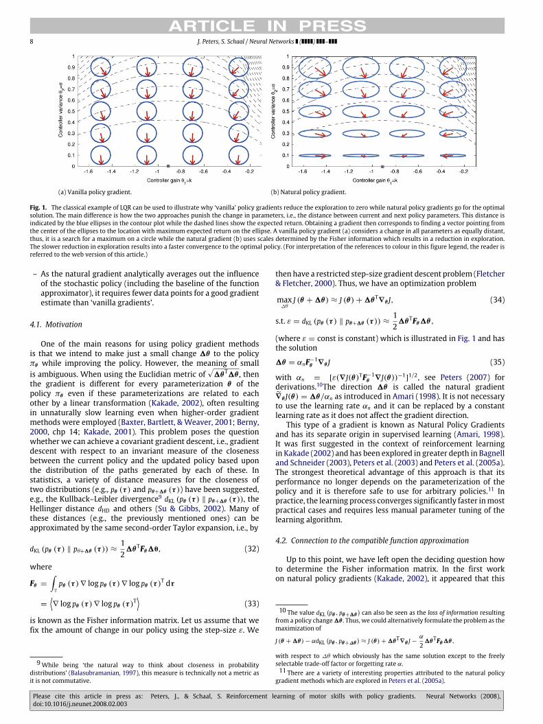
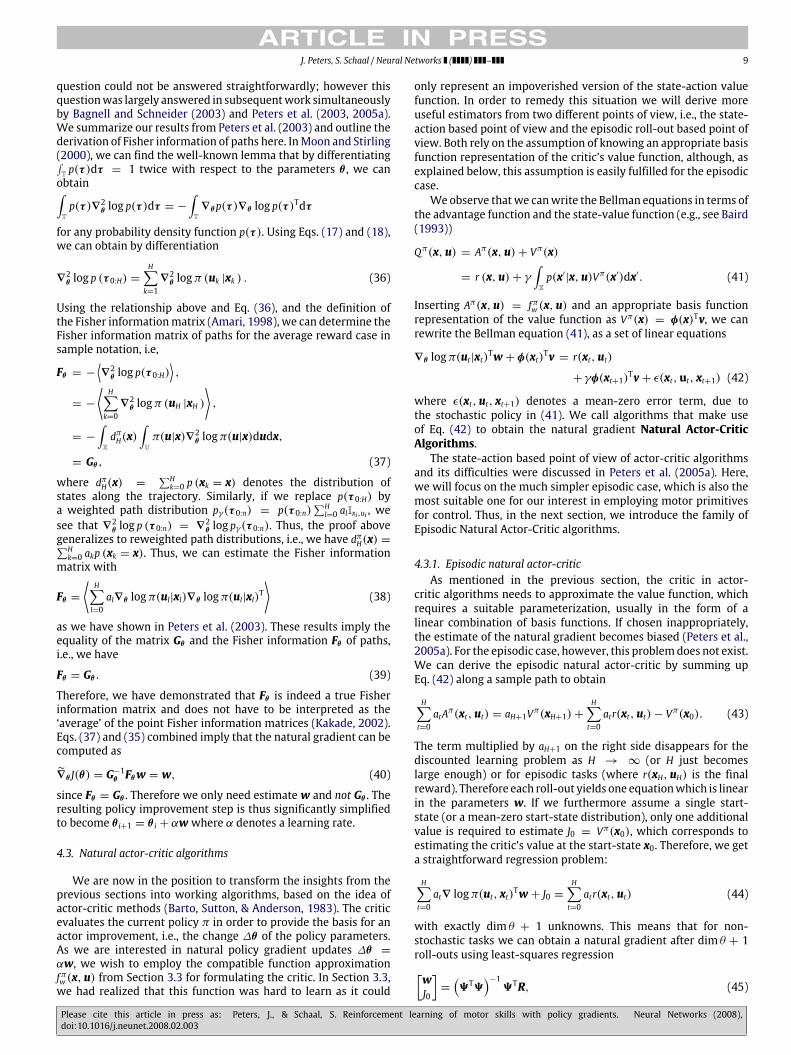
Example 2. The classical example of linear-quadratic regulationis surprisingly hard with ‘vanilla’ policy gradient approaches. Inthis problem, we have a linear system with Gaussian noise xt+1 ∼

N(Axt + But,σ

2x

), a linear policy with Gaussian exploration ut ∼

N (θ1xt, θ2) and a quadratic reward rt = −Qx2t − Ru2t . Traditionally‘vanilla’ policy gradient approaches decrease the exploration rateθ2 very fast and, thus, converge slowly towards the optimalsolution as illustrated in Fig. 1(a). The reason is that a decreaseof exploration has a stronger immediate effect on the expectedreturn. Thus, if both parameters are seen as independent (asindicated by the circles), the plateau at zero exploration will resultin the very slow convergence. If we can reweight the parameters,we could go along some directions faster than along others asindicated by the ellipses in Fig. 1(b). This reweighting can balanceexploration and exploitation, resulting in faster convergence to theoptimum. It is accomplished through the natural policy gradient.

This natural policy gradient approach was first suggested forreinforcement learning as the ‘average natural policy gradient’in Kakade (2002), and subsequently shown to be the true naturalpolicy gradient (Bagnell & Schneider, 2003; Peters, Vijayakumar,& Schaal, 2003). In this paper, we take this line of reasoning onestep further by introducing the Natural Actor-Critic which inheritsthe convergence guarantees from gradient methods. Severalproperties of the natural policy gradient are worth highlightingbefore investigating some of the relevant derivations:

– Convergence to a local minimum is guaranteed, see Amari(1998).

– By choosing a more direct path to the optimal solution in pa-rameter space, the natural gradient has, from empirical obser-vations, faster convergence and avoids premature convergenceof ‘vanilla gradients’ (see Fig. 1).

– The natural policy gradient can be shown to be covariant,i.e., independent of the coordinate frame chosen for expressingthe policy parameters, see Peters, Vijayakumar, and Schaal(2005b).



(a) Vanilla policy gradient. (b) Natural policy gradient.

Fig. 1. The classical example of LQR can be used to illustrate why ‘vanilla’ policy gradients reduce the exploration to zero while natural policy gradients go for the optimalsolution. The main difference is how the two approaches punish the change in parameters, i.e., the distance between current and next policy parameters. This distance isindicated by the blue ellipses in the contour plot while the dashed lines show the expected return. Obtaining a gradient then corresponds to finding a vector pointing fromthe center of the ellipses to the location with maximum expected return on the ellipse. A vanilla policy gradient (a) considers a change in all parameters as equally distant,thus, it is a search for a maximum on a circle while the natural gradient (b) uses scales determined by the Fisher information which results in a reduction in exploration.The slower reduction in exploration results into a faster convergence to the optimal policy. (For interpretation of the references to colour in this figure legend, the reader isreferred to the web version of this article.)

– As the natural gradient analytically averages out the influenceof the stochastic policy (including the baseline of the functionapproximator), it requires fewer data points for a good gradientestimate than ‘vanilla gradients’.

4.1. Motivation

One of the main reasons for using policy gradient methodsis that we intend to make just a small change 1θ to the policyπθ while improving the policy. However, the meaning of smallis ambiguous. When using the Euclidian metric of

√1θT1θ , then

the gradient is different for every parameterization θ of thepolicy πθ even if these parameterizations are related to eachother by a linear transformation (Kakade, 2002), often resultingin unnaturally slow learning even when higher-order gradientmethods were employed (Baxter, Bartlett, & Weaver, 2001; Berny,2000, chp 14; Kakade, 2001). This problem poses the questionwhether we can achieve a covariant gradient descent, i.e., gradientdescent with respect to an invariant measure of the closenessbetween the current policy and the updated policy based uponthe distribution of the paths generated by each of these. Instatistics, a variety of distance measures for the closeness oftwo distributions (e.g., pθ (τ ) and pθ+1θ (τ )) have been suggested,e.g., the Kullback–Leibler divergence9 dKL (pθ (τ ) ‖ pθ+1θ (τ )), theHellinger distance dHD and others (Su & Gibbs, 2002). Many ofthese distances (e.g., the previously mentioned ones) can beapproximated by the same second-order Taylor expansion, i.e., by

dKL (pθ (τ ) ‖ pθ+1θ (τ )) ≈121θTFθ1θ, (32)

where

Fθ =

∫Tpθ (τ )∇ log pθ (τ )∇ log pθ (τ )T dτ

=

⟨∇ log pθ (τ )∇ log pθ (τ )T

⟩(33)

is known as the Fisher information matrix. Let us assume that wefix the amount of change in our policy using the step-size ε. We

9While being ‘the natural way to think about closeness in probabilitydistributions’ (Balasubramanian, 1997), this measure is technically not a metric asit is not commutative.

then have a restricted step-size gradient descent problem (Fletcher& Fletcher, 2000). Thus, we have an optimization problem

max∆θ

J (θ +1θ) ≈ J (θ) +1θT∇θ J, (34)

s.t. ε = dKL (pθ (τ ) ‖ pθ+1θ (τ )) ≈121θTFθ1θ,

(where ε = const is constant) which is illustrated in Fig. 1 and hasthe solution

1θ = αnF−1θ ∇θ J (35)

with αn = [ε(∇J(θ)TF−1θ ∇J(θ))−1

]1/2, see Peters (2007) for

derivations.10The direction 1θ is called the natural gradient∇θ J(θ) = 1θ/αn as introduced in Amari (1998). It is not necessaryto use the learning rate αn and it can be replaced by a constantlearning rate as it does not affect the gradient direction.

This type of a gradient is known as Natural Policy Gradientsand has its separate origin in supervised learning (Amari, 1998).It was first suggested in the context of reinforcement learningin Kakade (2002) and has been explored in greater depth in Bagnelland Schneider (2003), Peters et al. (2003) and Peters et al. (2005a).The strongest theoretical advantage of this approach is that itsperformance no longer depends on the parameterization of thepolicy and it is therefore safe to use for arbitrary policies.11 Inpractice, the learning process converges significantly faster inmostpractical cases and requires less manual parameter tuning of thelearning algorithm.

4.2. Connection to the compatible function approximation

Up to this point, we have left open the deciding question howto determine the Fisher information matrix. In the first workon natural policy gradients (Kakade, 2002), it appeared that this

10 The value dKL(pθ , pθ+1θ

)can also be seen as the loss of information resulting

from a policy change1θ . Thus, we could alternatively formulate the problem as themaximization of

J (θ +1θ) − αdKL(pθ , pθ+∆θ

)≈ J (θ) +1θT∇θ J −

α

21θTFθ1θ,

with respect to ∆θ which obviously has the same solution except to the freelyselectable trade-off factor or forgetting rate α.11 There are a variety of interesting properties attributed to the natural policy

gradient methods which are explored in Peters et al. (2005a).



question could not be answered straightforwardly; however thisquestionwas largely answered in subsequentwork simultaneouslyby Bagnell and Schneider (2003) and Peters et al. (2003, 2005a).We summarize our results from Peters et al. (2003) and outline thederivation of Fisher information of paths here. InMoon and Stirling(2000), we can find the well-known lemma that by differentiating∫

T p(τ )dτ = 1 twice with respect to the parameters θ , we canobtain∫

Tp(τ )∇2

θ log p(τ )dτ = −

∫T∇θp(τ )∇θ log p(τ )Tdτ

for any probability density function p(τ ). Using Eqs. (17) and (18),we can obtain by differentiation

∇2θ log p (τ 0:H) =

H∑k=1

∇2θ logπ (uk |xk ) . (36)

Using the relationship above and Eq. (36), and the definition ofthe Fisher informationmatrix (Amari, 1998), we can determine theFisher information matrix of paths for the average reward case insample notation, i.e,

Fθ = −

⟨∇

2θ log p(τ 0:H)

⟩,

= −

⟨H∑

k=0∇

2θ logπ (uH |xH )

⟩,

= −

∫XdπH(x)

∫Uπ(u|x)∇2

θ logπ(u|x)dudx,

= Gθ , (37)

where dπH(x) =∑H

k=0 p (xk = x) denotes the distribution ofstates along the trajectory. Similarly, if we replace p(τ 0:H) bya weighted path distribution pγ(τ 0:n) = p(τ 0:n)

∑Hl=0 alIxi,ui , we

see that ∇2θ log p (τ 0:n) = ∇

2θ log pγ(τ 0:n). Thus, the proof above

generalizes to reweighted path distributions, i.e., we have dπH(x) =∑Hk=0 akp (xk = x). Thus, we can estimate the Fisher information

matrix with

Fθ =

⟨H∑

l=0al∇θ logπ(ul|xl)∇θ logπ(ul|xl)

T

⟩(38)

as we have shown in Peters et al. (2003). These results imply theequality of the matrix Gθ and the Fisher information Fθ of paths,i.e., we have

Fθ = Gθ . (39)

Therefore, we have demonstrated that Fθ is indeed a true Fisherinformation matrix and does not have to be interpreted as the‘average’ of the point Fisher information matrices (Kakade, 2002).Eqs. (37) and (35) combined imply that the natural gradient can becomputed as

∇θ J(θ) = G−1θ Fθw = w, (40)

since Fθ = Gθ . Therefore we only need estimate w and not Gθ . Theresulting policy improvement step is thus significantly simplifiedto become θ i+1 = θ i + αw where α denotes a learning rate.

4.3. Natural actor-critic algorithms

We are now in the position to transform the insights from theprevious sections into working algorithms, based on the idea ofactor-critic methods (Barto, Sutton, & Anderson, 1983). The criticevaluates the current policy π in order to provide the basis for anactor improvement, i.e., the change ∆θ of the policy parameters.As we are interested in natural policy gradient updates ∆θ =

αw, we wish to employ the compatible function approximationfπw (x,u) from Section 3.3 for formulating the critic. In Section 3.3,we had realized that this function was hard to learn as it could

only represent an impoverished version of the state-action valuefunction. In order to remedy this situation we will derive moreuseful estimators from two different points of view, i.e., the state-action based point of view and the episodic roll-out based point ofview. Both rely on the assumption of knowing an appropriate basisfunction representation of the critic’s value function, although, asexplained below, this assumption is easily fulfilled for the episodiccase.

We observe thatwe canwrite the Bellman equations in terms ofthe advantage function and the state-value function (e.g., see Baird(1993))

Qπ(x,u) = Aπ(x,u) + Vπ(x)

= r (x,u) + γ

∫Xp(x′

|x,u)Vπ(x′)dx′. (41)

Inserting Aπ(x,u) = fπw (x,u) and an appropriate basis functionrepresentation of the value function as Vπ(x) = φ(x)Tv, we canrewrite the Bellman equation (41), as a set of linear equations

∇θ logπ(ut|xt)Tw + φ(xt)

Tv = r(xt,ut)

+ γφ(xt+1)Tv + ε(xt,ut, xt+1) (42)

where ε(xt,ut, xt+1) denotes a mean-zero error term, due tothe stochastic policy in (41). We call algorithms that make useof Eq. (42) to obtain the natural gradient Natural Actor-CriticAlgorithms.

The state-action based point of view of actor-critic algorithmsand its difficulties were discussed in Peters et al. (2005a). Here,we will focus on the much simpler episodic case, which is also themost suitable one for our interest in employing motor primitivesfor control. Thus, in the next section, we introduce the family ofEpisodic Natural Actor-Critic algorithms.

4.3.1. Episodic natural actor-criticAs mentioned in the previous section, the critic in actor-

critic algorithms needs to approximate the value function, whichrequires a suitable parameterization, usually in the form of alinear combination of basis functions. If chosen inappropriately,the estimate of the natural gradient becomes biased (Peters et al.,2005a). For the episodic case, however, this problemdoes not exist.We can derive the episodic natural actor-critic by summing upEq. (42) along a sample path to obtain

H∑t=0

atAπ(xt,ut) = aH+1V

π(xH+1) +

H∑t=0

atr(xt,ut) − Vπ(x0). (43)

The term multiplied by aH+1 on the right side disappears for thediscounted learning problem as H → ∞ (or H just becomeslarge enough) or for episodic tasks (where r(xH,uH) is the finalreward). Therefore each roll-out yields one equationwhich is linearin the parameters w. If we furthermore assume a single start-state (or a mean-zero start-state distribution), only one additionalvalue is required to estimate J0 = Vπ(x0), which corresponds toestimating the critic’s value at the start-state x0. Therefore, we geta straightforward regression problem:

H∑t=0

at∇ logπ(ut, xt)Tw + J0 =

H∑t=0

atr(xt,ut) (44)

with exactly dim θ + 1 unknowns. This means that for non-stochastic tasks we can obtain a natural gradient after dim θ + 1roll-outs using least-squares regression[wJ0

]=

(9T9

)−19TR, (45)



Table 5Episodic natural actor-critic with a constant baseline


1 repeat2 perform M trials and obtain x0:H,u0:H, r0:H for each trial.

Obtain the sufficient statistics3 Policy derivatives ψk = ∇θ logπθ (uk |xk ).

4 Fisher matrix Fθ =

⟨(∑Hk=0 ψk

) (∑Hl=0 ψ l

)T⟩.

Vanilla gradient g =

⟨(∑Hk=0 ψk

) (∑Hl=0 alrl

)⟩.

5 Eligibility φ =

⟨(∑Hk=0 ψk

)⟩.

6 Average reward r =

⟨∑Hl=0 alrl

⟩.

Obtain natural gradient by computing7 Baseline b = Q

(r − φTF−1

θg)

with Q = M−1(1 + φT

(MFθ − φφT

)−1φ

)8 Natural gradient geNAC1 = F−1

θ (g − φb) .

9 until gradient estimate geNAC1 converged.

return: gradient estimate geNAC1 .

Table 6Episodic natural actor-critic with a time-variant baseline


1 repeat2 perform M trials and obtain x0:H,u0:H, r0:H for each trial.

Obtain the sufficient statistics3 Policy derivatives ψk = ∇θ logπθ (uk |xk ).4 Fisher matrix Fθ =

⟨∑Hk=0

(∑kl=0 ψ l

)ψT

k

⟩.

Vanilla gradient g =

⟨∑Hk=0

(∑kl=0 ψ l

)akrk

⟩,

5 Eligibility matrix8 = [φ1,φ2, . . . ,φK ]

with φh =

⟨(∑hk=0 ψk

)⟩.

6 Average reward vector r = [r1, r2, . . . , rK ]

with rh = 〈ahrh〉.Obtain natural gradient by computing

7 Baseline b = Q(r −8TF−1

θg)

with Q = M−1(IK +8T

(MFθ −88T

)−18

).

8 Natural gradient gNG = F−1θ (g −8b) .

9 until gradient estimate geNACn converged.

return: gradient estimate geNACn .

with

9 i =

[H∑

t=0at∇ logπ(ut, xt)

T, 1]

, (46)

Ri =

H∑t=0

atr(xt,ut). (47)

This regression problem, can be transformed into the form shownin Table 5 using the matrix inversion lemma, see Peters (2007) forthe derivation.

4.3.2. Episodic natural actor-critic with a time-variant baselineThe episodic natural actor-critic described in the previous

section suffers from one drawback: it does not make use ofintermediate reward data along the roll-out, just like REINFORCE.An improvement was suggested by G(PO)MDP, which left outterms which would average out in expectation. One can argue thatthis omission of terms is equivalent to using a time-dependentbaseline. We can make use of the same argument and reformulatethe Episodic Natural Actor-Critic which results in the algorithmshown in Table 6. The advantage of this type of algorithms is two-fold: the variance of the gradient estimate is often lower and it cantake time-variant rewards significantly better into account.

The time-variant baseline can also be seen in a slightly differentlight as it is not only a baseline but at the same time an additional

basis function for the critic. As we argued in the previous section, asingle constant offset suffices as additional basis function as it onlyneeds to represent the value of the first state (or the average of firststates as the start-state distribution does not dependon the policy).Obviously, using more basis functions than one constant offsetrepresenting the value of the first step can reduce the varianceof the gradient estimate even further without introducing bias.We know from the non-episodic Natural Actor-Critic, that if wehad large experience with the system and knew state-dependentbasis functions, we can obtain the much better gradient estimate.However, we also know that we rarely have these good additionalbasis functions. Nevertheless, in some problems, we stay closeto certain kinds of trajectories. In this important case, the state-dependent basis functions can be replaced by time-dependent ortime-variant basis functions with an equivalent result.

Nevertheless, if we have a time-variant baseline in an episodicsetup, this will increase the complexity of the current setup andthe regression problem has a solution

[geNACn

r

]=

[F2 8

8T

mIH

]−1 [gr

](48)

where we have a Fisher information matrix estimate Fθ =⟨∑Hk=0

(∑kl=0 ψ l

)ψT

k

⟩with log-policy derivatives ψk = ∇θ log

πθ (uk |xk ), the vanilla gradient estimate g =

⟨∑Hk=0

(∑kl=0 ψ l

)akrk

⟩,

an eligibility matrix 8 = [φ1,φ2, . . . ,φK] with φh =

⟨(∑hk=0 ψk

)⟩and r = [r1, r2, . . . , rK] with rh = 〈ahrh〉. Computing geNACn thusinvolves the inversion of a matrix which has the size H+ n, i.e., thesum of the episode length H and parameters n. Obviously, sucha matrix is prone to be ill-conditioned if inverted with a brute-force approach and computationally expensive. Nevertheless, asthis matrix contains the identity matrix IH in the largest block ofthe matrix, we can reduce the whole problem to an inversion of amatrix which has the number of policy parameters n as size. Whenmaking use of thematrix inversion theorem (using Harville (2000),pages 98–101, or Moon and Stirling (2000), pages 258–259; fordetails see also Peters (2005)), we can simplify this approach to

w = β1 = F−12

(g − 8b

)= F−1

2 g2, (49)

b = β2 = Q−1(r − 8

TF−12 g

), (50)

with Q−1= m−1(In + 8

T(mF2 − 88

T)−18). This algorithm is

depicted in Table 6, and detailed derivations can be found in Peters(2005).

5. Empirical evaluations

In the previous section, we outlined five model-free policygradient algorithms. From our assessment, these are among themost relevant for learning motor primitives in robotics as they canbe applied without requiring additional function approximationmethods and as they are suitable for episodic settings. Thesealgorithms were (i) finite-difference gradient estimators, thevanilla policy gradient estimators (ii) with a constant baseline and(iii) a time-variant baseline, as well as the episodic Natural Actor-Critic with both (iv) an offset as additional basis functions and (v)a time-variant offset as additional basis functions.

In this section, we will demonstrate how the differentalgorithms compare in practice. For this purpose, we will showexperiments on both a simulated plant as well as on a real robotandwewill compare the algorithms for the optimization of controllaws and for learning of motor skills.



5.1. Comparing policy gradient methods on motor primitives

Our goal in this section is to evaluate policy gradient methodsfor the applicability to learning motor primitives. As outlinedin Section 1.2, we are interested in two different kinds ofrepresentations, i.e., a spline-based and dynamical systems.

In a spline-based approach (e.g., Miyamoto et al. (1996) andSciavicco and Siciliano (2007)), we have a series of concatenatedsplines, which together form a desired trajectory — third-ordersplines or fifth-order splines are among the most popular choices.Boundary conditions between the individual splines ensuresmooth trajectories with continuous derivatives up to a certainorder, which are determined by the order of the spline polynomial.Depending on the design principle, the splines can have equal ordifferent durations. The pros of spline-based trajectory planningare the ease of use of splines and the compact representationthat consists only of the spline boundary conditions and timing.Among the main short-comings (Miyamoto et al., 1996; Sciavicco& Siciliano, 2007) are that between spline nodes, splines cansometimes create rather complex and undesirable behavior, andthat the explicit time indexing of splines makes it hard to have on-linemodifications of the spline plan, e.g., in terms of potential fieldsdue to obstacle avoidance. We included spline-based trajectoryplanning as a base-line comparison for our learning algorithms,as the spline parameters are perfectly suited as a representationfor parameterized movement primitives. In our implementation,we used third-order splines of equal time duration to spanthe desired movement duration. Third-order splines have fourboundary conditions, i.e., position and velocity at each node, andbetween splines, the boundary conditions of the ending spline arethe same as those of the starting spline. We chose six splines forthe entire trajectory, resulting in a total of 10 free parameters (thestart and end conditions of the desired trajectory are given).

As an alternative to splines, a dynamical system approach wassuggested in Ijspeert et al. (2002, 2003). The basic principle hereis that a by-design globally stable attractor system automaticallycreates a desired trajectory through its unfolding in time. Giventhat the dynamical system is autonomous, potential fields caneasily be incorporated to allow for on-line modification of thedesired trajectory, e.g., due to the need of obstacle avoidance.Additionally, scaling in speed and amplitude of movement is easilyaccomplished, derived from a framework of structural equivalenceof dynamical systems. One dynamical system motor primitiverepresents a large family of movements, as it is valid for any initialcondition. More details on this approach can be found in Appendixor in Ijspeert et al. (2002, 2003). The open parameters in thedynamical systemmotor primitive are the coefficients of a functionapproximator with linear parameters (cf. Appendix). As we usedten basis functions in the function approximator, we obtained 10free parameters in the motor primitive, i.e., the same number offree parameters as in the spline approach.

We compared the algorithms (i)–(v) in four different scenarios.Each of these scenarios consists of the usage of one of the kinematicplan representations (i.e., splines or motor primitives) and twodifferent tasks. Each task represents a motor plan in joint spacerepresentedby joint angle q andvelocity q. These taskswere chosensuch thatwe can evaluate the different policy gradientmethods forlearning standard motor primitives as they appear frequently inthe motor control literature (Ben-Itzhak & Karniel, in press; Flash& Hochner, 2005) as well as for applicability in the T-ball taskpresented in Section 5.2. The optimal policies for these tasks can befound in the literature, e.g., in Ben-Itzhak and Karniel (in press) andFlash and Hochner (2005). In all the experiments in this section,we used a single Degree-of-Freedom (DoF) scenario for the easeof illustration. To optimize the performance, we improved everygradient estimator as much as possible. Therefore each algorithm

has learning rates that were manually chosen to maximize theperformance while not destabilizing the gradient descent. In orderto curb the variance of the gradient estimates, we make useof the PEGASUS trick (Ng & Jordan, 2000) for the generationof exploration (i.e., the perturbation of our motor commands isachieved using the same history of random numbers). All othersettings were optimized in order to make each of these algorithmsas good as possible, e.g., the random perturbation frequency ofthe different algorithms is tuned for maximum performance, asperturbations at too high frequency result in very slow learning,and perturbations at too low frequency can destabilize motorcontrol.

The first task is to achieve a goal with a minimum-squaredmovement acceleration and a given movement duration, i.e., areward of

r(x0:H,u0:H) = −

H/2∑i=0

c1q2i −

H∑i= H

2 +1

c2[(qi − g)2 + q2i ] (51)

is being optimized, where c1 = 1/100 is the weight of thetransient rewards for the movement duration H/2, while c2 =

1000 is the importance of the final reward, extended over thetime interval [H/2 + 1,H], which insures that the goal state g =

1.0 is reached and maintained properly. The start-state of themotor primitive is always zero in this toy evaluation. The optimalmovement with respect to this reward is known to be a third-order polynomial in time, with boundary conditions set accordingto the movement start and goal (Ben-Itzhak & Karniel, in press).We use this analytically optimal solution as a baseline, which isunachievable for the motor primitives due to the pre-requisiteof smooth acceleration profiles — the third-order spline optimalsolution has discontinuous accelerations at the start and end of themovement.

In Fig. 2, the task and the different solutions are illustrated. Forthe spline representation, all algorithms achieve the same goodresult. For the motor primitives, the best solution is a very closeapproximation of the analytically optimal solutions. The finite-differencemethods do not reach this optimal solution but get stuckin a local minimum.

The second task involves passing through an intermediate pointduring the trajectory, while minimizing the squared accelerations,i.e., we have a similar reward with an additional punishment termfor missing the intermediate point pF at time F given by

r(x0:H,u0:H) = −

H/2∑i=0

c1q2i −

H∑i=H/2+1

c2[(qi − g)2 + q2i ]

− c3(qF − pF)2, (52)

where c1 = 1, c2 = 20, c3 = 20 000. The goal has a value of g = 1,the intermediate point a value of pF = 0.5 at F = 7H/20 andthe start-state was zero. This reward yields a smooth movementwhich first passes through the intermediate point before reachingthe goal. This toy experiment is in preparation for hitting a baseballin the robot experiment below.

In Fig. 3, the second task and the different solutions areillustrated. Again, we compare against the analytically optimalsolution described by two third-order splines, whose velocityboundary conditions at the intermediate point are optimizedaccording to the minimum-squared acceleration cost. As in thefirst task, the motor primitives can only approximate this optimalsolution due to smoothness constraints of the acceleration profiles.The results are very similar as those for the first task: for themotor primitives, a good approximation of the analytically optimalsolution is achieved by all but the finite-difference method, whichseems to get stuck in local minima. The spline representationshows no significant differences among the five different learning



Fig. 2. This figure illustrates the task accomplished in the minimum motorcommand learning example. In (a, b), the positions of splines and motor primitivesare shown, in (c, d) the velocities and in (e, f) the accelerations. The cyandashed line shows the initial configurations, which is accomplished by straight-line movement initializations for the splines, and zero parameters for the motorprimitives. The dash-dotted dark blue line shows the analytically optimal solution,which is unachievable for the motor primitives, but nicely approximated by theirbest solution, presented by the red solid line. This best solution is reached by alllearning methods except for the finite-difference method, which gets stuck in alocal minimum — shown as the green dashed line. The wiggly curve in the middleof the motor primitive acceleration results from the basis function approximationof this curve with Gaussian basis functions — the number of wiggles correspondsto the number of basis functions. The spline representation achieves very close tooptimal results for all algorithms. The legend is given in (g). (For interpretationof the references to colour in this figure legend, the reader is referred to the webversion of this article.)

methods, but the learned trajectory does not quite coincide withthe optimal solution, as none of the spline nodes correspondedexactly to the intermediate point pF .

While the trajectory plots do not really distinguish the differentlearning algorithms, except for the finite-difference method,the learning curves demonstrate significant and interestingdifferences. In Fig. 4(a) and (b), we show a comparison for thefirst task (goal achievement with a minimum-squared motorcommand) for both splines and dynamic motor primitives,respectively. In Fig. 4(c) and (d) we show similar plots for the taskwith the intermediate target. These comparisons clearly establishthat both versions of the episodic natural actor-critic methodsoutperform both the vanilla policy gradient methods as well as

Fig. 3. This figure illustrates the results when learning to pass through anintermediate point while having smooth motion. In (a, b), the positions of splinesandmotor primitives are shown, in (c, d) the velocities and in (e, f) the accelerations.The dashed cyan line shows the initial configurations, which is accomplished bystraight-line movement initializations for the splines, and zero parameters for themotor primitives. The dash-dotted dark blue line shows the analytically optimalsolution, which is unachievable for the motor primitives, but nicely approximatedby their best solution, presented by the red solid line. This best solution is reachedby all learningmethods except for the finite-differencemethod, which gets stuck ina local minimum — shown as the green dashed line. The best solution achieved bylearning is presented by the red solid line, which was very close to the analyticallyoptimal one. The legend is given in (g). (For interpretation of the references to colourin this figure legend, the reader is referred to the web version of this article.)

the finite-differencemethods. The difference between the episodicnatural actor-critic methods with single-offset and the time-variant additional basis functions is relatively small; however, forpractical tasks this can still make a significant difference. Thetime-invariant baseline barely improves over the constant baselinefor the vanilla policy gradients. For finite-difference gradientmethods, it is best not to apply exploration during the trajectorybut only perturb the parameters at the start of the episode.Otherwise, the gradient estimate is too noisy for any practicalpurposes. While this lack of exploration results into an increasedaccuracy of the gradient, the lack of stochasticity in the systemresults in an increase of plateaus and local minima (Ng & Jordan,2000; Spall, 2003). This problem could be overcome by collectingsufficiently many samples with additional stochastic, exploratory



Fig. 4. This figure shows different experiments with learning motor tasks. In(a, b), we see how the learning system creates plans for the minimum motorcommand cost using both (a) splines and (b) motor primitives. For this problem,the natural actor-critic methods learns the optimal solution faster by several ordersof magnitude than any of the other methods. In (c, d), the plan has to achieve anintermediary goal. While the natural actor-critic methods still outperform previousmethods, the gap is lower as the learning problem is easier. Note that these aredouble logarithmic plots. Both ‘vanilla’ policy gradient methods and natural onesachieve the same final solution — just at a different pace. Finite-difference methodson the other hand often do not attain a similarly good solution as in (a, d).

actions, but at the cost of many more roll-outs. Both vanilla policygradient methods and the natural actor-critic methods avoid these

local minima due to the usage of exploratory actions instead ofparameter perturbations.

From the results presented in Fig. 4(a–d), we conclude thatnatural actor-critic methods seem to have a significant advantagefor our learning goals, i.e., optimizing the parameters of controlpolicies.

5.2. Robot application: Motor primitive learning for baseball

In this section, we apply the Episodic Natural Actor-Critic in amulti-DOF robot motor learning task, using a Sarcos Master Arm.The task of the robot is to hit a (soft) baseball placed on a T-sticksuch that it flies as far as possible — this game is also known as T-Ball and is used in theUS to teach childrenhow tohit a baseball. Thestate of the robot is given by its joint angles and velocities whilethe actions are the joint accelerations. A given inverse dynamicscontroller is used to obtain motor torques from these kinematicvariables. The ball position and velocity are observed through acolor vision system (Newton Labs, MA) at 60 Hz video frequency.

There are several complex components in this setup. Theball has to be hit at a proper location and proper angle withmaximal velocity while avoiding to saturate the robot torques— this is modeled by minimizing the squared motor commands,i.e., acceleration of the motor primitives. Additionally, the taskhas to be distributed appropriately among the seven degrees offreedom of the robot, which are redundant during the hittingmovement. As each degree of freedomhas a singlemotor primitiverepresenting its behavior over time, the redundancies require twoimplementational simplifications. The first simplification is theusage of the same randomnumber generator for exploration acrossall seven motor primitives. This simplification is well known tointroduce similar exploration over all degrees of freedom and hasbeen shown to reduce the variance in the gradient estimate (Fu,2002). It is necessary, as otherwise the exploration noise addedin one DOF will often “fight” the exploration noise of other DOFs,resulting in very slow learning. Second, we need to cope witha 70-dimensional Fisher information matrix, which is hard tostabilize numerically. However, it is a reasonable assumption thatthis Fisher information matrix is dominated by its block diagonalas the parameters of the same motor primitive are more tightlycoupled than between different motor primitives. This results intotreating themotor primitive of eachDOF as if they could be learnedindependently, i.e., we do not need to treat all the parameters ofall motor primitives as one big optimization problem. Note thatthis approximation of the Fisher information matrix is positivedefinite and, thus, inherits all convergence guarantees from the‘vanilla’ policy gradients while still yielding speeds comparable toan implementation of the Episodic Natural Actor-Critic withoutthis simplification. The joint reward signal for eachmotor primitivefor degree of freedom k was

rk(x0:H,u0:H) = +c1px −

H∑i=0

c2q2k;i (53)

where px denotes the distance of the ball travelled (as estimatedfrom the equations of a ballistic flight using initial trajectorycaptured by the vision system — the scope of the vision systemwas zoomed in the area around the ball to obtain high resolutioninformation and could not see where the ball landed) along thex-axis while q2

k;i punishes high joint accelerations of joint k at timei, where the weight of each cost component is given by c1 = 1000,c2 = 1. Note, that for a single DoF this Eq. (53) would be amore abstract version of Eq. (52). As policy gradient methods arelocal learning methods, we cannot expect to learn this complex,high-dimensional behavior in a short time unless we initialize themotor primitives with some prior knowledge. For motor control,



(a) Performance. (b) Imitation learning. (c) Initial reproduction. (d) After reinforcementlearning.

Fig. 5. This figure shows (a) the average of the reward, Eq. (53), over all DoFs of the baseball swing task when using the motor primitives for learning. In (b), the learningsystem is initialized by imitation learning, in (c) it is initially failing at reproducing the motor behavior, and (d) after several hundred episodes exhibiting a nicely learnedbatting, which achieves about 5 m distance of the ball flight.

a suitable approach is to first imitate a teacher and, subsequently,improve by trial and error. This setup mimics how children learnhow to a hit a baseball where first the parent presents and,subsequently, the child improves on its own. Similarly, we use theone-shot supervised learning setup12 presented in Ijspeert et al.(2002, 2003) to teach the robot a rudimentary T-ball stroke as canbe seen in Fig. 5(b); however, it fails to reproduce the behavior asshown in (c) due to control inaccuracies of the robot; subsequently,we improve the accuracy of the hitting angle using the episodicNatural Actor-Criticwhich yields the performance shown in (a) andthe behavior in (d). After approximately 200–300 trials, the ball canbe hit properly by the robot.

6. Conclusion & discussion

We have presented an extensive survey of policy gradientmethods. While some developments needed to be omitted as theyare only applicable for very low-dimensional state-spaces, thispaper largely summarized the state of the art in policy gradientmethods as applicable in robotics with high degree-of-freedommovement systems. All the three major ways of estimating first-order gradients, i.e., finite-difference gradients, vanilla policygradients and natural policy gradients are discussed in this paperand practical algorithms are given.

One of the presented classes of algorithms, the Natural Actor-Critic algorithms was developed for this paper. This class ofalgorithms has been widely accepted by now and has been appliedin a variety of settings (Guenter, Hersch, Calinon, & Billard, inpress; Mori et al., 2004; Mori, Nakamura, & Ishii, 2005; Nakamuraet al., 2004; Park, Kim, & Kang, 2005; Richter, Aberdeen, & Yu,2007; Sato et al., 2002; Ueno et al., 2006). The Natural Actor-Critic is considered the “Current method of choice” (Aberdeen,2006) among the policy gradient methods in the reinforcementlearning community. It also allows the derivation of severalpreviously presented algorithms in the literature and has veryuseful theoretical properties (Peters, 2007).

The experiments presented here show that the time-variantepisodic natural actor-critic is the preferred method among thepresentedmethodswhen applicable; however, if a policy cannot bedifferentiated with respect to its parameters, the finite-differencemethodsmaybe the onlymethod applicable. The example ofmotorprimitive learning for baseball underlines the efficiency of naturalgradient methods for complex movement systems.

12 This setup first extracts the duration of the desired movement and adjusts alltime constants of the motor primitives. Based on the resulting dynamical systems,it computes the targets for the a locally weighted regression performed based onLWPR. See Ijspeert et al. (2002, 2003) for all details on this approach.

Appendix. Motor primitive equations

The motor primitives from Ijspeert et al. (2002, 2003) in theirmost recent reformulation are given by a canonical system

τ−1v = αv (βv (g − x) − v) , (A.1)

τ−1x = v, (A.2)

which represents the phase of the motor process. It has a goal g,a time constant τ and some parameters αv,βv which are chosenso that the system is stable. Additionally, we have a transformedsystem

τ−1z = αz (βz (s − x) − v) + f (x, v, g) , (A.3)

τ−1y = z, (A.4)

τ−1 s = αs (g − s) , (A.5)

which has the same time constant τ as the canonical system,appropriately set parameters αz,βz,αs, and a transformationfunction f (x, v, g). The transformation function transforms theoutput of the canonical system so that the transformed system canrepresent complex nonlinear patterns and is given by

f (x, v, g) =

N∑i=1ψi (x) θiv

N∑i=1ψi (x)

, (A.6)

where θi are adjustable parameters and it has localization weightsdefined by

ψi (x) = exp(−hi

(x − x0g − x0

− ci

)2)

(A.7)

with offset x0, centers ci and width hi.

References

Aberdeen, D. (2006). POMDPs and policy gradients, presentation at the MachineLearning Summer School (MLSS).

Aleksandrov, V., Sysoyev, V., & Shemeneva, V. (1968). Stochastic optimization.Engineering Cybernetics, 5, 11–16.

Amari, S. (1998). Natural gradient works efficiently in learning.Neural Computation,10, 251.

Atkeson, C. G. (1994). Using local trajectory optimizers to speed up globaloptimization in dynamic programming. In J. E. Hanson, S. J. Moody, &R. P. Lippmann (Eds.), Advances in neural information processing systems 6(pp. 503–521). Morgan Kaufmann.

Bagnell, J., & Schneider, J. (2003). Covariant policy search. In Proceedings of theinternational joint conference on artificial intelligence (pp. 1019–1024).

Baird, L. (1993). Advantage updating. Technical Report WL-TR-93-1146. Wrightlaboratory, Wright–Patterson air force base. OH.

Balasubramanian, V. (1997). Statistical inference, occam’s razor, and statisticalmechanics on the space of probability distributions. Neural Computation, 9(2),349–368.



Barto, A. G., Sutton, R. S., & Anderson, C. W. (1983). Neuronlike adaptive elementsthat can solve difficult learning control problems. IEEE Transactions on Systems,Man, and Cybernetics SMC, 13(5), 115–133.

Baxter, J., & Bartlett, P. (2001). Infinite-horizon policy-gradient estimation. Journalof Artificial Intelligence Research, 15, 319–350.

Baxter, J., Bartlett, P., &Weaver, L. (2001). Experimentswith infinite-horizon, policy-gradient estimation. Journal of Artificial Intelligence Research, 15, 351–381.

Ben-Itzhak, S., & Karniel, A. (2008).Minimumacceleration criterionwith constraintsimplies bang–bang control as an underlying principle for optimal trajectories ofarm reaching movements. Neural Computation, 20(3), 779–812.

Benbrahim, H., Doleac, J., Franklin, J., & Selfridge, O. (1992). Real-time learning:A ball on a beam. In Proceedings of the international joint conference on neuralnetworks (pp. 92–103).

Benbrahim, H., & Franklin, J. (1997). Biped dynamic walking using reinforcementlearning. Robotics and Autonomous Systems, 22, 283–302.

Berny, A. (2000). Statistical machine learning and combinatorial optimization.In Lecture notes in natural computing: Vol. 33 (pp. 287–306). Heidelberg,Germany: Springer-Verlag.

Dyer, P., & McReynolds, S. R. (1970). The computation and theory of optimal control.New York, NY: Academic Press.

Endo, G., Morimoto, J., Matsubara, T., Nakanishi, J., & Cheng, G. (2005). Learningcpg sensory feedback with policy gradient for biped locomotion for a full-bodyhumanoid. In Proceedings of the national conference on artificial intelligence (pp.1267–1273).

Flash, T., & Hochner, B. (2005). Motor primitives in vertebrates and invertebrates.Current Opinions in Neurobiology, 15, 660–666.

Fletcher, R., & Fletcher, R. (2000). Practical methods of optimization. New York, NY:John Wiley & Sons.

Fu, M. C. (2002). Feature article: Optimization for simulation: Theory vs. practice.INFORMS Journal on Computing, 14(3), 192–215.

Glynn, P. (1987). Likelihood ratio gradient estimation: An overview. In Proceedingsof the winter simulation conference (pp. 366–375).

Glynn, P. (1990). Likelihood ratio gradient estimation for stochastic systems.Communications of the ACM, 33(10), 75–84.

Greensmith, E., Bartlett, P., & Baxter, J. (2001). Variance reduction techniques forgradient estimates in reinforcement learning. Advances in Neural InformationProcessing Systems, 14(34).

Greensmith, E., Bartlett, P. L., & Baxter, J. (2004). Variance reduction techniquesfor gradient estimates in reinforcement learning. Journal of Machine LearningResearch, 5, 1471–1530.

Guenter, F., Hersch, M., Calinon, S., & Billard, A. (2007). Reinforcement learning forimitating constrained reaching movements. In Imitative Robots [Special issue].RSJ Advanced Robotics, 21, 1521–1544.

Gullapalli, V. (1990). A stochastic reinforcement learning algorithm for learningreal-valued functions. Neural Networks, 3(6), 671–692.

Gullapalli, V. (1992). Learning control under extreme uncertainty. In Advances inneural information processing systems (pp. 327–334).

Gullapalli, V., Franklin, J., & Benbrahim, H. (1994). Aquiring robot skills viareinforcement learning. IEEE Control Systems Journal, Special Issue on Robotics:Capturing Natural Motion, 4(1), 13–24.

Harville, D. A. (2000). Matrix algebra from a statistician’s perspective. Heidelberg,Germany: Springer Verlag.

Hasdorff, L. (1976). Gradient optimization and nonlinear control. New York, NY: JohnWiley & Sons.

Ijspeert, J.A., Nakanishi, J., & Schaal, S. (2002). Movement imitation with nonlineardynamical systems in humanoid robots. In Proceedings of IEEE internationalconference on robotics and automation (pp. 1398–1403).

Ijspeert, A., Nakanishi, J., & Schaal, S. (2003). Learning attractor landscapes forlearning motor primitives. In S. Becker, S. Thrun, & K. Obermayer (Eds.),Advances in neural information processing systems: Vol. 15 (pp. 1547–1554).Cambridge, MA: MIT Press.

Jacobson, D. H., & Mayne, D. Q. (1970). Differential dynamic programming. New York,NY: American Elsevier Publishing Company, Inc.

Kakade, S. (2001). Optimizing average reward using discounted rewards. InProceedings of the conference on computational learning theory (pp. 605–615).

Kakade, S. A. (2002). Natural policy gradient. In Advances in neural informationprocessing systems: Vol. 14 (pp. 1531–1538). CA: Vancouver.

Kakade, S.M. (2003). On the sample complexity of reinforcement learning. Ph.D.thesis, Gatsby computational Neuroscience Unit. University College London,London, UK.

Kimura, H., & Kobayashi, S. (1997). Reinforcement learning for locomotion of a two-linked robot arm. In Proceedings of the Europian workshop on learning robots (pp.144–153).

Kimura, H., & Kobayashi, S. (1998). Reinforcement learning for continuous actionusing stochastic gradient ascent. In Proceedings of the international conferenceon intelligent autonomous systems (IAS): Vol. 5 (pp. 288–295).

Kleinman, N., Spall, J., & Naiman, D. (1999). Simulation-based optimizationwith stochastic approximation using common random numbers. ManagementScience, 45, 1570–1578.

Kohl, N., & Stone, P. (2004). Policy gradient reinforcement learning for fastquadrupedal locomotion. In Proceedings of the IEEE international conference onrobotics and automation (pp. 2619–2624).

Konda, V., & Tsitsiklis, J. (2000). Actor-critic algorithms. Advances in NeuralInformation Processing Systems, 12.

Lawrence, G., Cowan, N., & Russell, S. (2003). Efficient gradient estimation formotorcontrol learning. In Proceedings of the international conference on uncertainty inartificial intelligence (pp. 354–361).

Mitsunaga, N., Smith, C., Kanda, T., Ishiguro, H., & Hagita, N. (2005). Robot behavioradaptation for human-robot interaction based on policy gradient reinforcementlearning. In Proceedings of the IEEE/RSJ international conference on intelligentrobots and systems (pp. 1594–1601).

Miyamoto, H., Gandolfo, F., Gomi, H., Schaal, S., Koike, Y., & Osu, R. et al. (1995). Akendama learning robot based on a dynamic optimization theory. In Proceedingsof the IEEE international workshop on robot and human communication (pp.327–332).

Miyamoto, H., Gandolfo, F., Gomi, H., Schaal, S., Koike, Y., & Rieka, O. et al. (1996).A kendama learning robot based on a dynamic optimization principle. InProceedings of the international conference on neural information processing (pp.938–942).

Moon, T., & Stirling, W. (2000). Mathematical methods and algorithms for signalprocessing. Upper Saddle River, NJ: Prentice Hall.

Mori, T., Nakamura, Y., aki Sato, M., & Ishii, S. (2004). Reinforcement learning forcpg-driven biped robot. In Proceedings of the national conference on artificialintelligence (pp. 623–630).

Mori, T., Nakamura, Y., & Ishii, S. (2005). Efficient sample reuse by off-policy naturalactor-critic learning. In Advances in neural information processing systems (NIPS’05 workshop presentation).

Morimoto, J., & Atkeson, C. A. (2003). Minimax differential dynamic programming:an application to robust biped walking. In S. Becker, S. Thrun, & K. Obermayer(Eds.), Advances in neural information processing systems 15 (pp. 1539–1546).Cambridge, MA: MIT Press.

Nakamura, Y., Mori, T., & Ishii, S. (2004). Natural policy gradient reinforcementlearning for a CPG control of a biped robot. In Proceedings of the internationalconference on parallel problem solving from nature (pp. 972–981).

Nakanishi, J., Morimoto, J., Endo, G., Cheng, G., Schaal, S., & Kawato, M. (2004).Learning from demonstration and adaptation of biped locomotion. Robotics andAutonomous Systems, 47(2–3), 79–91.

Ng, A.Y., & Jordan, M. (2000). PEGASUS: A policy search method for large MDPs andPOMDPs. In Proceedings of the international conference on uncertainty in artificialintelligence (pp. 406–415).

Park, J., Kim, J., & Kang, D. (2005). An RLS-based natural actor-critic algorithm forlocomotion of a two-linked robot arm. In Y. Hao, J. Liu, Y.Wang, Y. ming Cheung,H. Yin, L. Jiao, J. Ma, & Y.-C. Jiao (Eds.), Lecture notes in computer science: Vol.3801. Proceedings of the international conference on computational intelligenceand security (CIS) (pp. 65–72). Xi’an, China: Springer.

Peters, J. (2005). Machine learning of motor skills for robotics. Technical Report CS-05-867. University of Southern California, Los Angeles, CA.

Peters, J. (2007).Machine learning ofmotor skills for robotics. Ph.D. thesisUniversityof Southern California, Los Angeles, CA, 90089, USA.

Peters, J., & Schaal, S. (2006). Policy gradient methods for robotics. In Proceedingsof the IEEE/RSJ international conference on intelligent robots and systems (pp.2219–2225).

Peters, J., Vijayakumar, S., & Schaal, S. (2003). Reinforcement learning for humanoidrobotics. In Proceedings of the IEEE-RAS international conference on humanoidrobots (HUMANOIDS) (pp. 103–123).

Peters, J., Vijayakumar, S., & Schaal, S. (2005a). Natural actor-critic. In Proceedings ofthe European machine learning conference (pp. 280–291).

Peters, J., Vijayakumar, S., & Schaal, S. (2005b). Natural actor-critic. In Proceedings ofthe European conference on machine learning (pp. 280–291). Springer.

Pongas, D., Billard, A., & Schaal, S. (2005). Rapbid synchronization and accuratephase-locking of rhythmic motor primitives. In Proceedings of the IEEEinternational conference on intelligent robots and systems (IROS 2005): Vol. 2005(pp. 2911–2916).

Richter, S., Aberdeen, D., & Yu, J. (2007). Natural actor-critic for road trafficoptimisation. In B. Schoelkopf, J. Platt, & T. Hofmann (Eds.), Advances in neuralinformation processing systems: Vol. 19. Cambridge, MA: MIT Press, p. OnlinePreproceedings.

Sadegh, P., & Spall, J. (1997). Optimal random perturbations for stochasticapproximation using a simultaneous perturbation gradient approximation. InProceedings of the american control conference (pp. 3582–3586).

Sato, M., Nakamura, Y., & Ishii, S. (2002). Reinforcement learning for bipedlocomotion. In Lecture notes in computer science, Proceedings of the internationalconference on artificial neural networks (ICANN) (pp. 777–782). Springer-Verlag.

Schaal, S. (1997). Learning from demonstration. In M. Mozer, M. Jordan, & T.Petsche (Eds.), Advances in neural information processing systems (NIPS): Vol. 9(pp. 1040–1046). Cambridge, MA: MIT Press.

Schaal, S., Peters, J., Nakanishi, J., & Ijspeert, A. (2004). Learning movementprimitives. In Springer tracts in advanced robotics, International symposium onrobotics research (ISRR2003) (pp. 561–572). Ciena, Italy: Springer.

Sciavicco, L., & Siciliano, B. (2007). Modeling and control of robot manipulators.Heidelberg, Germany: MacGraw-Hill.

Spall, J. C. (2003). Introduction to stochastic search and optimization: Estimation,simulation, and control. Hoboken, NJ: Wiley.

Su, F., & Gibbs, A. (2002). On choosing and bounding probability metrics.International Statistical Review, 70(3), 419–435.

Sutton, R. S., McAllester, D., Singh, S., &Mansour, Y. (2000). Policy gradient methodsfor reinforcement learningwith function approximation. In S. A. Solla, T. K. Leen,& K.-R. Mueller (Eds.), Advances in neural information processing systems (NIPS)(pp. 1057–1063). Denver, CO: MIT Press.

Tedrake, R., Zhang, T.W., & Seung, H.S. (2005). Learning to walk in 20 min. InProceedings of the Yale workshop on adaptive and learning systems (pp. 10–22).Yale University, New Haven, New Haven, CT.



Ueno, T., Nakamura, Y., Takuma, T., Shibata, T., Hosoda, K., & Ishii, S. (2006). Fastand stable learning of quasi-passive dynamic walking by an unstable bipedrobot based on off-policy natural actor-critic. In Proceedings of the IEEE/RSJinternational conference on intelligent robots and systems (pp. 5226–5231).

Vachenauer, P., Rade, L., & Westergren, B. (2000). Springers Mathematische Formeln:Taschenbuch für Ingenieure, Naturwissenschaftler, Informatiker, Wirtschaftswis-senschaftler. Heidelberg, Germany: Springer-Verlag.

Wada, Y., & Kawato, M. (1994). Trajectory formation of arm movement by a neuralnetwork with forward and inverse dynamics models. Systems and Computers inJapan, 24, 37–50.

Weaver, L., & Tao, N. (2001a). The optimal reward baseline for gradient-basedreinforcement learning. In: Proceedings of the international conference onuncertainty in artificial intelligence (pp. 538–545). Vol. 17. Seattle, Washington.

Weaver, L., & Tao, N. (2001b). The variance minimizing constant reward baseline forgradient-based reinforcement learning. Technical Report 30. Australian NationalUniversity (ANU).

Werbos, P. (1979). Changes in global policy analysis procedures suggested by newmethods of optimization. Policy Analysis and Information Systems, 3(1).

Williams, R. J. (1992). Simple statistical gradient-following algorithms forconnectionist reinforcement learning.Machine Learning, 8(23).


reinforcement learning of motor skills with policy gradients

Documents