reinforcement learning in self organizing cellular networks
TRANSCRIPT

REINFORCEMENT LEARNING IN SELF ORGANIZING
CELLULAR NETWORKS
by
Roohollah Amiri
A dissertation
submitted in partial fulfillment
of the requirements for the degree of
Doctor of Philosophy in Electrical and Computer Engineering
Boise State University
May 2020

© 2020Roohollah Amiri
ALL RIGHTS RESERVED

BOISE STATE UNIVERSITY GRADUATE COLLEGE
DEFENSE COMMITTEE AND FINAL READING APPROVALS
of the dissertation submitted by
Roohollah Amiri
Dissertation Title: Reinforcement Learning In Self Organizing Cellular Networks
Date of Oral Examination: 29 May 2020
The following individuals read and discussed the dissertation submitted by studentRoohollah Amiri, and they evaluated the presentation and response to questionsduring the final oral examination. They found that the student passed the final oralexamination.
Hani Mehrpouyan, Ph.D. Chair, Supervisory Committee
John Chiasson, Ph.D. Member, Supervisory Committee
Hao Chen, Ph.D. Member, Supervisory Committee
Erik Perrins, Ph.D. External Examiner
The final reading approval of the dissertation was granted by Hani Mehrpouyan,Ph.D., Chair of the Supervisory Committee. This dissertation was approved by theGraduate College.

To my parents who sacrificed too much for me.
iv

ACKNOWLEDGMENTS
I am using this opportunity to express my gratitude to my advisor Dr. Hani
Mehrpouyan for his support, guidance, and friendship during the last five years. Dr.
Mehrpouyan is one of the sharpest people I know who despite his intelligence does not
have a bigoted attitude. Dr. Mehrpouyan always gave me freedom on choosing my
research topics and people who I worked with. He always shows genuine excitement
in my ideas and supports them on many different levels from idea to analysis and
implementation. Dr. Mehrpouyan’s scrutiny on writing and presentation of ideas
has improved my writing skills enormously. His willingness to collaborate with other
researchers has made many opportunities for me. I thank him for his patience in
reviewing my papers, and generosity of sharing his technical material with me.
My sincere gratitude goes to Professor Jeffrey G. Andrews who agreed to host me
at the University of Texas at Austin for about a year in 2019. Working with Professor
Andrews has been a pivot point in my career. During my visit at UT Austin, I had
many valuable meetings and discussions with Prof. Andrews and I am grateful for
such experience.
I would like to extend my gratitude towards my committee members, Dr. John
Chiasson and Dr. Hao Chen. I always enjoyed my technical discussions with them
during courses that I took with them. My sincere thanks goes to Dr. Chiasson for
his effort in developing great courses in machine learning. I would like to use this
opportunity to thank Jenn Ambrose, the ECE department manager, and all her staff.
v

I have had the chance to work with brilliant researchers during my PhD as
collaborations on different projects and technical papers. Here, my sincere thanks
goes to Professor David Matolak at the University of South Carolina, Dr. Maged
Elkashlan at Queen Mary University of London, Dr. Lex Fridman at Massachusetts
Institute of Technology, Professor Ranjan K. Mallik at Indian Institute of Technology,
Professor Arumugam Nallanathan at Kings College London, Dr. Eren Balevi at
University of Texas at Austin, and Dr. Mojtaba Vaezi at Villanova University.
Special thanks to Dr. Solmaz Niknam, Mojtaba Ahmadi Almasi, and Ruthvik
Vaila as my lab mates and close friends and for many technical discussions, argu-
ments, and laughter. I also thank all the lab members and former visitors of High
Performance Computing lab for creating a nice environment for research. I have to
thank my group mates at UT Austin for great meetings and technical discussions.
My special thanks go to my friends Ahmad AlAmmouri, Anum Ali, and Rebal Jurdi
who made my visit at UT Austin memorable.
When it comes to living in a foreign country, friends have the potential to be your
family. I have been privileged for having such friends who I call family now, Zachariah
Vandeventer and Isabella Cohen and their beautiful families. My special thanks goes
to Zachariah who has been my partner in crime during my life in Boise. Further, my
gratitude goes to Bahareh Badamchi who always treated me with kindness.
Finally and most importantly, I thank my family back home for their unconditional
support, their unwavering confidence in my abilities and their encouragement in all
of my endeavors. My unconditional love goes to my sister and brother who I wish all
the best for. Without you, this journey would not have been possible.
vi

ABSTRACT
Self-organization is a key feature as cellular networks densify and become more
heterogeneous, through the additional small cells such as pico and femtocells. Self-
organizing networks (SONs) can perform self-configuration, self-optimization, and
self-healing. These operations can cover basic tasks such as the configuration of a
newly installed base station, resource management, and fault management in the
network. In other words, SONs attempt to minimize human intervention where they
use measurements from the network to minimize the cost of installation, configuration,
and maintenance of the network. In fact, SONs aim to bring two main factors
in play: intelligence and autonomous adaptability. One of the main requirements
for achieving such goals is to learn from sensory data and signal measurements in
networks. Therefore, machine learning techniques can play a major role in processing
underutilized sensory data to enhance the performance of SONs.
In the first part of this dissertation, we focus on reinforcement learning as a viable
approach for learning from signal measurements. We develop a general framework in
heterogeneous cellular networks agnostic to the learning approach. We design multiple
reward functions and study different effects of the reward function, Markov state
model, learning rate, and cooperation methods on the performance of reinforcement
learning in cellular networks. Further, we look into the optimality of reinforcement
learning solutions and provide insights into how to achieve optimal solutions.
In the second part of the dissertation, we propose a novel architecture based on
vii

spatial indexing for system-evaluation of heterogeneous 5G cellular networks. We
develop an open-source platform based on the proposed architecture that can be used
to study large scale directional cellular networks. The proposed platform is used for
generating training data sets of accurate signal-to-interference-plus-noise-ratio (SINR)
values in millimeter-wave communications for machine learning purposes. Then,
with taking advantage of the developed platform, we look into dense millimeter-wave
networks as one of the key technologies in 5G cellular networks. We focus on topology
management of millimeter-wave backhaul networks and study and provide multiple
insights on the evaluation and selection of proper performance metrics in dense
millimeter-wave networks. Finally, we finish this part by proposing a self-organizing
solution to achieve k-connectivity via reinforcement learning in the topology manage-
ment of wireless networks.
viii

TABLE OF CONTENTS
Abstract . . . . . . . . . . . . . . . . . . . . . . . . . . . . . . . . . . . . . . . . . . . . . . . . . . vii
List of Tables . . . . . . . . . . . . . . . . . . . . . . . . . . . . . . . . . . . . . . . . . . . . . . xiv
List of Figures . . . . . . . . . . . . . . . . . . . . . . . . . . . . . . . . . . . . . . . . . . . . . xv
LIST OF ABBREVIATIONS . . . . . . . . . . . . . . . . . . . . . . . . . . . . . . . . . xviii
1 Introduction . . . . . . . . . . . . . . . . . . . . . . . . . . . . . . . . . . . . . . . . . . . . . 1
1.1 The Road to 5G . . . . . . . . . . . . . . . . . . . . . . . . . . . . . . . . . . . . . . . . . . . 2
1.2 Self-Organizing Networks . . . . . . . . . . . . . . . . . . . . . . . . . . . . . . . . . . . . 4
1.3 SON Requirements and Reinforcement Learning . . . . . . . . . . . . . . . . . . 6
1.4 Challenges . . . . . . . . . . . . . . . . . . . . . . . . . . . . . . . . . . . . . . . . . . . . . . . 9
1.5 Summary of Contributions . . . . . . . . . . . . . . . . . . . . . . . . . . . . . . . . . . . 10
1.6 Dissertation Organization . . . . . . . . . . . . . . . . . . . . . . . . . . . . . . . . . . . . 15
2 Reinforcement Learning for Power Control of Two-Tier Heteroge-
neous Networks . . . . . . . . . . . . . . . . . . . . . . . . . . . . . . . . . . . . . . . . . . 16
2.1 Introduction . . . . . . . . . . . . . . . . . . . . . . . . . . . . . . . . . . . . . . . . . . . . . . 17
2.1.1 Related Work . . . . . . . . . . . . . . . . . . . . . . . . . . . . . . . . . . . . . . . 18
2.1.2 Contributions . . . . . . . . . . . . . . . . . . . . . . . . . . . . . . . . . . . . . . . 20
2.2 Downlink System Model . . . . . . . . . . . . . . . . . . . . . . . . . . . . . . . . . . . . . 22
2.3 Problem Formulation . . . . . . . . . . . . . . . . . . . . . . . . . . . . . . . . . . . . . . . 24
ix

2.4 The Proposed Learning Framework . . . . . . . . . . . . . . . . . . . . . . . . . . . . 26
2.4.1 Multi-Agent MDP and Policy Evaluation . . . . . . . . . . . . . . . . . . 26
2.4.2 Factored MDP . . . . . . . . . . . . . . . . . . . . . . . . . . . . . . . . . . . . . . 29
2.4.3 Femtocell Network as Multi-Agent MDP . . . . . . . . . . . . . . . . . . 31
2.5 Q-DPA, Reward Function, and Sample Complexity . . . . . . . . . . . . . . . . 34
2.5.1 Q-learning Based Distributed Power Allocation (Q-DPA) . . . . . 34
2.5.2 Proposed Reward Function . . . . . . . . . . . . . . . . . . . . . . . . . . . . . 38
2.5.3 Sample Complexity . . . . . . . . . . . . . . . . . . . . . . . . . . . . . . . . . . . 44
2.6 Simulation Results . . . . . . . . . . . . . . . . . . . . . . . . . . . . . . . . . . . . . . . . . 45
2.6.1 Simulation Setup . . . . . . . . . . . . . . . . . . . . . . . . . . . . . . . . . . . . . 46
2.6.2 Performance of Q-DPA . . . . . . . . . . . . . . . . . . . . . . . . . . . . . . . . 48
2.6.3 Reward Function Performance . . . . . . . . . . . . . . . . . . . . . . . . . . 51
2.7 Conclusion . . . . . . . . . . . . . . . . . . . . . . . . . . . . . . . . . . . . . . . . . . . . . . . 53
3 Power Allocation in Interference-Limited Networks via Coordinated
Learning . . . . . . . . . . . . . . . . . . . . . . . . . . . . . . . . . . . . . . . . . . . . . . . . 54
3.1 Introduction . . . . . . . . . . . . . . . . . . . . . . . . . . . . . . . . . . . . . . . . . . . . . . 55
3.1.1 Related Work . . . . . . . . . . . . . . . . . . . . . . . . . . . . . . . . . . . . . . . 56
3.1.2 Contributions . . . . . . . . . . . . . . . . . . . . . . . . . . . . . . . . . . . . . . . 56
3.2 System Model . . . . . . . . . . . . . . . . . . . . . . . . . . . . . . . . . . . . . . . . . . . . . 57
3.3 Problem Analysis . . . . . . . . . . . . . . . . . . . . . . . . . . . . . . . . . . . . . . . . . . 58
3.3.1 Problem Analysis . . . . . . . . . . . . . . . . . . . . . . . . . . . . . . . . . . . . 59
3.3.2 Nash Equilibrium and Pareto Optimality . . . . . . . . . . . . . . . . . . 60
3.4 Distributed Coordinated Q-learning . . . . . . . . . . . . . . . . . . . . . . . . . . . . 61
3.4.1 Optimal Solution via Q-learning . . . . . . . . . . . . . . . . . . . . . . . . . 61
x

3.4.2 Factored MDP . . . . . . . . . . . . . . . . . . . . . . . . . . . . . . . . . . . . . . 63
3.4.3 Decomposition of Global Q-function . . . . . . . . . . . . . . . . . . . . . . 64
3.4.4 Coordinated Action Selection . . . . . . . . . . . . . . . . . . . . . . . . . . . 65
3.4.5 Local Update Rule . . . . . . . . . . . . . . . . . . . . . . . . . . . . . . . . . . . 68
3.5 Power Allocation Using Coordinated Q-Learning . . . . . . . . . . . . . . . . . . 68
3.5.1 Q-CoPA Algorithm . . . . . . . . . . . . . . . . . . . . . . . . . . . . . . . . . . . 69
3.5.2 Q-learning Configurations . . . . . . . . . . . . . . . . . . . . . . . . . . . . . . 70
3.6 Simulation Results . . . . . . . . . . . . . . . . . . . . . . . . . . . . . . . . . . . . . . . . . 70
3.7 Conclusion . . . . . . . . . . . . . . . . . . . . . . . . . . . . . . . . . . . . . . . . . . . . . . . 72
4 Spatial Indexing for System-Level Evaluation of 5G Heterogeneous
Cellular Networks . . . . . . . . . . . . . . . . . . . . . . . . . . . . . . . . . . . . . . . . 74
4.1 Introduction . . . . . . . . . . . . . . . . . . . . . . . . . . . . . . . . . . . . . . . . . . . . . . 74
4.1.1 Contributions . . . . . . . . . . . . . . . . . . . . . . . . . . . . . . . . . . . . . . . 75
4.1.2 Motivation . . . . . . . . . . . . . . . . . . . . . . . . . . . . . . . . . . . . . . . . . . 76
4.1.3 Related Works . . . . . . . . . . . . . . . . . . . . . . . . . . . . . . . . . . . . . . . 77
4.2 Spatial Indexing and Queries in HetNets . . . . . . . . . . . . . . . . . . . . . . . . 79
4.2.1 Architecture . . . . . . . . . . . . . . . . . . . . . . . . . . . . . . . . . . . . . . . . 79
4.2.2 Indexing a HetNet With single Geometry Tree . . . . . . . . . . . . . . 80
4.2.3 Spatial Queries . . . . . . . . . . . . . . . . . . . . . . . . . . . . . . . . . . . . . . 82
4.3 Simulation Acceleration with Spatial Indexing . . . . . . . . . . . . . . . . . . . . 86
4.3.1 SNR calculation . . . . . . . . . . . . . . . . . . . . . . . . . . . . . . . . . . . . . 87
4.3.2 SINR calculation . . . . . . . . . . . . . . . . . . . . . . . . . . . . . . . . . . . . . 88
4.4 Conclusion . . . . . . . . . . . . . . . . . . . . . . . . . . . . . . . . . . . . . . . . . . . . . . . 89
xi

5 Topology Management in Millimeter Wave Wireless Backhaul in 5G
Cellular Networks . . . . . . . . . . . . . . . . . . . . . . . . . . . . . . . . . . . . . . . . 90
5.1 Introduction . . . . . . . . . . . . . . . . . . . . . . . . . . . . . . . . . . . . . . . . . . . . . . 91
5.1.1 Related Work . . . . . . . . . . . . . . . . . . . . . . . . . . . . . . . . . . . . . . . 93
5.1.2 Contributions . . . . . . . . . . . . . . . . . . . . . . . . . . . . . . . . . . . . . . . 96
5.2 System Model . . . . . . . . . . . . . . . . . . . . . . . . . . . . . . . . . . . . . . . . . . . . . 97
5.2.1 Antenna Model . . . . . . . . . . . . . . . . . . . . . . . . . . . . . . . . . . . . . . 98
5.2.2 Path Loss . . . . . . . . . . . . . . . . . . . . . . . . . . . . . . . . . . . . . . . . . . 99
5.2.3 Interference Model . . . . . . . . . . . . . . . . . . . . . . . . . . . . . . . . . . . 100
5.3 Distributed Path Selection . . . . . . . . . . . . . . . . . . . . . . . . . . . . . . . . . . . 100
5.3.1 Path selection policies . . . . . . . . . . . . . . . . . . . . . . . . . . . . . . . . . 101
5.3.2 Effect of selecting SNR vs SINR as mmWave link quality metric 101
5.4 K-Connectivity with Multi-Agent Reinforcement Learning . . . . . . . . . . 105
5.4.1 Q-learning for range control . . . . . . . . . . . . . . . . . . . . . . . . . . . . 106
5.4.2 Resulted topology . . . . . . . . . . . . . . . . . . . . . . . . . . . . . . . . . . . . 107
5.5 Conclusion . . . . . . . . . . . . . . . . . . . . . . . . . . . . . . . . . . . . . . . . . . . . . . . 110
6 Conclusion . . . . . . . . . . . . . . . . . . . . . . . . . . . . . . . . . . . . . . . . . . . . . . 111
6.1 Summary . . . . . . . . . . . . . . . . . . . . . . . . . . . . . . . . . . . . . . . . . . . . . . . . 111
6.2 Future Research Direction . . . . . . . . . . . . . . . . . . . . . . . . . . . . . . . . . . . 114
6.2.1 Deep reinforcement learning for large state sets . . . . . . . . . . . . . 114
6.2.2 Mean-field reinforcement learning in large networks . . . . . . . . . . 114
6.2.3 Spatial correlation of blocking in HetNets . . . . . . . . . . . . . . . . . . 115
6.2.4 Graph embedding in topology management . . . . . . . . . . . . . . . . 115
Bibliography . . . . . . . . . . . . . . . . . . . . . . . . . . . . . . . . . . . . . . . . . . . . . . . 116
xii

Appendices . . . . . . . . . . . . . . . . . . . . . . . . . . . . . . . . . . . . . . . . . . . . . . . . 128
A Chapter 2 . . . . . . . . . . . . . . . . . . . . . . . . . . . . . . . . . . . . . . . . . . . . . . . 129
A.1 Proof of Proposition 1 . . . . . . . . . . . . . . . . . . . . . . . . . . . . . . . . . . . . . . 130
B Chapter 4 . . . . . . . . . . . . . . . . . . . . . . . . . . . . . . . . . . . . . . . . . . . . . . . 135
B.1 Insertion to the R-tree . . . . . . . . . . . . . . . . . . . . . . . . . . . . . . . . . . . . . . 136
B.2 Parallel processing and message-passing . . . . . . . . . . . . . . . . . . . . . . . . . 137
B.3 SINR characterization . . . . . . . . . . . . . . . . . . . . . . . . . . . . . . . . . . . . . . 139
C Chapter 5 . . . . . . . . . . . . . . . . . . . . . . . . . . . . . . . . . . . . . . . . . . . . . . . 141
C.1 Synchronous and Asynchronous Learning . . . . . . . . . . . . . . . . . . . . . . . . 142
xiii

LIST OF TABLES
2.1 Urban dual strip pathloss model . . . . . . . . . . . . . . . . . . . . . . . . . . . . . . 46
2.2 Simulation Parameters . . . . . . . . . . . . . . . . . . . . . . . . . . . . . . . . . . . . . . 46
2.3 Performance of different learning configurations. 1 is the best, and 4
is the worst. . . . . . . . . . . . . . . . . . . . . . . . . . . . . . . . . . . . . . . . . . . . . . . 51
5.1 Notation, Simulation Parameters . . . . . . . . . . . . . . . . . . . . . . . . . . . . . . 99
5.2 Path selection policies for wireless mmWave backhauling. . . . . . . . . . . . 101
5.3 Simulation Parameters . . . . . . . . . . . . . . . . . . . . . . . . . . . . . . . . . . . . . . 108
xiv

LIST OF FIGURES
1.1 Agent and environment interaction in RL . . . . . . . . . . . . . . . . . . . . . . . 8
2.1 Macrocell and femtocells operating over the same frequency band. . . . . 23
2.2 The proposed learning framework: the environment from the point of
view of an agent (FBS), and its interaction with the environment in
the learning procedure. Context defines the data needed to derive the
state of the agent. Measurement refers to calculations needed to derive
the reward of the agent. . . . . . . . . . . . . . . . . . . . . . . . . . . . . . . . . . . . . . 32
2.3 Reward functions: (a) Proposed reward function with m = 2, (b)
Quadratic reward function with zero maximum at (4.0, 0.5), (c) Expo-
nential reward function, (d) Proximity reward function. . . . . . . . . . . . . 43
2.4 Dense urban scenario with a dual strip apartment block located at
distance of 350 m of the MBS; FUEs are randomly located inside each
apartment. . . . . . . . . . . . . . . . . . . . . . . . . . . . . . . . . . . . . . . . . . . . . . . . 45
2.5 Performance of different learning configurations: (a) transmission rate
of the MUE, (b) sum transmission rate of the FUEs, (c) sum transmit
power of the FBSs. . . . . . . . . . . . . . . . . . . . . . . . . . . . . . . . . . . . . . . . . . 49
2.6 Performance of the proposed reward function compared to quadratic,
exponential and proximity reward functions: (a) transmission rate of
the MUE, (b) sum transmission rate of the FUEs, (c) sum transmit
power of the FBSs. . . . . . . . . . . . . . . . . . . . . . . . . . . . . . . . . . . . . . . . . . 52
xv

3.1 Coordination graph. . . . . . . . . . . . . . . . . . . . . . . . . . . . . . . . . . . . . . . . . 64
3.2 Message passing. . . . . . . . . . . . . . . . . . . . . . . . . . . . . . . . . . . . . . . . . . . . 64
3.3 Global action-value function. . . . . . . . . . . . . . . . . . . . . . . . . . . . . . . . . . 71
3.4 Normalized throughput versus portion of interference (β). . . . . . . . . . . . 72
4.1 The proposed multi-level architecture. Location and geometry prop-
erties of elements of the network are abstracted in the Node object.
The Container stores the elements of the network on a geometry tree.
From the view of the geometry tree, all elements are the same and
represented as polygons. The Network basically represents any wireless
network which can be a WSN, mmWave, or an integrated access and
backhaul (IAB) network. . . . . . . . . . . . . . . . . . . . . . . . . . . . . . . . . . . . . 79
4.2 Example of a HetNet indexed with a single R-tree with n = 10 and
M = 3. (a) The tree containing different levels of MBRs which
partition a network of one macro BS (MBS), four SBSs, four UEs,
and one blockage. (b) The rectangles R1 to R17 represent MBRs, the
black MBRs (R1, R2) are the roots, the red MBRs (R3-R7) are the
second layer, and the green MBRs (R8-R17) are the leaf nodes which
contain the data objects of the network. The MBRs R1 and R2 cover
total area of the network. . . . . . . . . . . . . . . . . . . . . . . . . . . . . . . . . . . . . 81
4.3 (a) The value pairs of the R-tree leaves and their relationship with
the elements of the network. Each leaf contains location and a pointer
which stores the Node information of the respective element of the
network. Here, R14 contains the location of a SBS and its Node data.
(b) Retrieving higher levels of an object from a query result. . . . . . . . . 82
xvi

4.4 (a) Sectored-pattern antenna model with the beamwidth of φm, main-
lobe gain of Gmax, and side-lobe gain of Gmin. (b) Polygon estimating
the area in which potential interferer BSs reside. . . . . . . . . . . . . . . . . . . 84
4.5 (a) Processing times to calculate SNR of all existing links. (b) Loading
time to generate and store all nodes. . . . . . . . . . . . . . . . . . . . . . . . . . . . 87
4.6 Processing time to calculate SINR of all existing links. . . . . . . . . . . . . . 88
5.1 Deployment models of mmWave base stations with density of 100 SBS/km2.
MBSs are connected to the core network with a wired backhaul. SBSs
use wireless backhauling to reach one of the MBSs. PPP distribution
for SBSs and fixed locations for MBSs. . . . . . . . . . . . . . . . . . . . . . . . . . 98
5.2 The selected paths by following each of the four policies. The red nodes
represent the wired BS, black nodes represent the wireless SBSs. The
number on each BS shows the number of hops it takes to reach to a
wired BS. This number is zero for a wired BS and −1 for the ones with
no route to a wired BS. . . . . . . . . . . . . . . . . . . . . . . . . . . . . . . . . . . . . . 103
5.3 Empirical CDF over 1000 number of iterations for a fixed topology and
6 number of wired BSs. . . . . . . . . . . . . . . . . . . . . . . . . . . . . . . . . . . . . . 104
5.4 Topology of the network. The number on each node represents its degree.109
C.1 Independent process of an agent and the main process. . . . . . . . . . . . . . 142
C.2 Running time for training of the WSN with 62 sensors. The running
time for one process refers to synchronous learning and the rest are re-
lated to asynchronous learning. The machine specification for running
the simulations is Intel(R) Xeon(R) CPU E5-2683 [email protected]. . . . . . . 143
xvii
LIST OF ABBREVIATIONS
SON – Self Organizing Network
RL – Reinforcement Learning
MARL – Multi Agent Reinforcement Learning
HetNet – Heterogeneous Network
MBS – Macro Base Station
SBS – Small Base Station
FBS – Femto Base Station
UE – User Equipment
FUE – Femto User Equipment
MUE – Macro User Equipment
SNR – Signal to Noise Ratio
SINR – Signal to Interference plus Noise Ratio
DL – Deep Learning
DNN – Deep Neural Network
MDP – Markov Decision Process
mmWave – Millimeter Wave
WSN – Wireless Sensor Network
xviii
RAN – Radio Access Network
MIMO – Multiple Input Multiple Output
LoS – Line of Sight
NLoS – Non Line of Sight
IL – Independent Learning
CL – Cooperative Learning
CSI – Channel State Information
xix

1
Chapter 1
INTRODUCTION
Self-organizing network (SON) technology minimizes the cost of running a mobile
network by eliminating manual configuration of network elements at the time of
deployment, through dynamic optimization and troubleshooting during operation.
Further, SON improves network performance, customer experience, and reduces the
cost of mobile operator services. SON started as an approach to improve performance
of cellular radio access network (RAN) deployment and optimization in 2008. How-
ever, its focus is gradually extending beyond RAN to managing the core network as
well. Largely driven by the increasing complexity of new wireless network generation
(5G), multi-RAN, densification, and spectrum heterogeneity, global investments in
SON technology are expected to grow. By the end of 2022, the research estimates
that SON will account for a market worth 5.5 Billion dollars [1].
One of the new developments in SON is increasing its capabilities in self-learning
through artificial intelligence techniques. Self-learning is considered to be critical
to address 5G requirements. Reinforcement learning [2] is one of the most used
approaches from machine learning to make self-learning algorithms viable in SON.
This dissertation focuses on developing frameworks, algorithms, and platforms to
integrate reinforcement learning methods into algorithms designed for cellular net-
works. This chapter reviews some of the technologies of 5G, features of SON, and

2
reasons of interest in reinforcement learning. Then, the challenges of developing
a reinforcement learning algorithm are described. Finally, the contributions of the
dissertation are detailed.
1.1 The Road to 5G
5G is expected to provide multiple folds of data capacity, higher security and better
QoS in the next decade. Many new technologies will rely on 5G such as Virtual reality
(VR), augmented reality (AR), streaming services such as Chromecast or SanDisk,
and connected cars such as OnStar or Autonet. To realize such a vision, three key
technologies are under development: millimeter wave (mmWave) communications,
massive multiple-input multiple-output (MIMO), and ultra-densificiation [3].
To achieve higher rates promised for 5G there is just one way: Going up in
frequency. The mmWave frequency range between 30-300 GHz is almost unused and
can provide bandwidth on the range of GHz for communication. However, to be able
to use mmWave frequencies, new technologies needed to be developed at link-level
and new algorithms need to be designed at the system-level.
Severe path loss at mmWave frequencies was a barrier to not consider it for
wireless communication for a long time. However, thanks to the short wavelength
at mmWave frequencies, directivity can be achieved by using a large number of
antennas at transmitters and receivers to mitigate severe path loss [4]. MmWave
has been considered for short-range communications (such as Wi-Fi connections).
Further, cost-efficient mmWave communication in cellular networks is promised in
a few years. Three beamforming architectures have been proposed for mmWave
systems: digital [4], analog [5], and hybrid [6]. Hybrid beamforming is achieved with

3
different architectures such as: (i) hybrid beamforming with phase-shifters [6], (ii)
hybrid beamforming with lens antennas [7], and (iii) hybrid beamforming with recon-
figurable microelectromechanical systems (MEMS) integrated antennas [8]. Ahmadi
et. al. have developed new architecture (RA-MIMO) based on lens antennas to
generate multiple independent beams simultaneously using a single RF chain [9–11].
RA-MIMO is used to combat small-scale fading and shadowing in mmWave bands.
Further, multiple new antenna designs to steer the beam at mmWave frequencies are
proposed at [12–14].
At the system-level, one of the basic while effective ways to increase the capacity of
a cellular network is to make cells smaller. Cell shrinking results in reusing frequency
spectrum across a geographical area and less competition for users over resources.
Technically there is no limitation on reducing the cell size, even until the point in
which each access point just services one user [3]. In general, ultra densification is one
main technology to achieve higher data rates. Densification is achieved using nested
cells which is the use of low-range small base stations to provide better coverage or
higher capacity for the users. These small cells can be picocells (range below 100m),
or femtocells (Wi-Fi range). Meanwhile, achieving the full potential of densification
to improve the spectral efficiency of access links runs into the significant bottleneck
of efficient backhauling.
Wired and wireless technologies can be used as backhaul solutions. Wired tech-
nologies such as fiber or xDSL have the advantage of high throughput, high relia-
bility, and low latency. However, wired solutions have high expenses and situational
impracticality in providing backhaul to a large number of small cells [15]. On the
contrary, wireless technology is a potential solution to provide a cost-efficient and
scalable backhaul support when a wired solution is impractical [16, 17]. Wireless

4
backhaul technologies can operate at Sub6GHz or mmWave bands. Sub6GHz wireless
backhaul has the advantage of non-line-of-sight (NLoS) transmission with the disad-
vantage of co-channel interference and variable delay. In contrast, thanks to a large
spectrum, high directional transmission, and low delay of line-of-sight (LoS) links,
mmWave communications can be modeled as pseudo-wired communications without
interference [18]. Therefore, mmWave communications are suitable candidates for the
backhaul of dense small cells.
Considering the above, 5G will be heterogeneous on the access and backhaul
networks. Further, the number of nodes in a 5G network will increase in multiple
folds. As 5G gets more complex, network management procedures need to evolve
as well. In the following, we look into the SON as a viable solution for 5G network
management.
1.2 Self-Organizing Networks
As 5G networks get more complex, the management of such a system becomes a
challenge. In wireless networks, many network elements and associated parameters
are manually configured. Planning, commissioning, configuration, and management
of these parameters are essential for efficient and reliable network operation. Manual
tuning has limitations such as:
• Specialized expertise must be maintained to tune network parameters.
• The existing manual process is time-consuming and error-prone.
• Manual tuning results in long delays in response to the often rapidly-changing
network topologies and operating conditions.

5
• Manual tuning results in sub-optimal network performance.
Considering the above, the big picture vision for the management of large cellular
networks raised some questions: Could future networks become intelligent and orga-
nize their operations autonomously? What is the definition of intelligence/learning?
How do existing nodes adapt their operating parameters when a new node is added
(removed) to (from) the network? Such discussion was the introduction of the SON
concept in cellular networks.
SON has been discussed and defined in many parts of the literature. Here, we
bring our favorite definitions:
• SONs are intelligent systems which learn from environment and adapt to
statistical variations [19].
• A phenomenon in which nodes work cooperatively in response to changes in
the environment in order to achieve certain goals [20].
• A set of entities that obtain a global system behavior as a result of local
interactions without central control [21].
In cellular networks, SON refers to scalable, stable, and agile mobile network
automation to minimize human intervention with three main features: (i)
scalability: bounded complexity with respect to network size, (ii) stability: transition
from current state to desired state in limited time, and (iii) agility: transition
should not be sluggish! In cellular networks, SON aims for improving the network
performance while reducing capital and operational expenditures (CAPEX/OPEX).
Self-organization is a key feature as cellular networks densify and become more
heterogeneous, through the additional small cells such as pico and femtocells. SON’s

6
operations are defined at the deployment phase (self-configuration), optimization
phase (self-optimization), and maintenance phase (self-healing) [22]. These operations
can cover basic tasks such as the configuration of a newly installed base station,
resource management, and fault management in the network [23].
1.3 SON Requirements and Reinforcement Learning
One of the requirements of self-organization in cellular networks is open-loop com-
munication. This means that a transmitter has only access to a channel quality
indicator (CQI) signal received from its related receiver. CQI can be translated
into signal-to-interference-plus-noise-ration (SINR). Hence, on a high-level definition,
many problems in SON can be translated to making the transmitter intelligent enough
to configure/adapt itself based on SINR measurements. Further, intelligence can be
defined as learning a function/map from measurements (data samples) to a required
parameter. For instance, if pi stands for transmit power for the (i − 1)th SINR
measurement (γi−1), self-learning as a power control problem can be defined as follows.
Definition 1. For a given dataset (γi, pi)mi=1 drawn from fixed and unknown distri-
bution ρ (Γ,P), find a function f such that
f (γi−1) = pi, i = 1, ...,m. (1.1)
The above definition relates to the concept of statistical learning or more com-
monly known as machine learning.
The problem in Definition 1 has the following challenges:

7
• All signal measurements are not available at the transmitter at once. Hence,
the data set needs to be acquired during interaction with the receiver (or
environment).
• Correct outputs are unknown. In supervised learning algorithms, the correct
label (pi) for input (γi−1) is known. However, here there is no model of the
network at the transmitter and calculation of correct transmit power potentially
ends in a non-convex problem depending on channel coefficients.
• The transmitter needs to adapt the mapping function continuously due to the
changes in wireless channels.
Considering the above challenges, reinforcement learning (RL) is a promising
approach to attack the problem. RL is a branch of machine learning that concerns
with finding an optimal policy to interact with an unknown environment. In RL, the
environment is defined as a Markov decision process (MDP) and policy is defined as a
mapping between the MDP states and the actions taken at those states [24]. In each
time step, t, an agent takes an action (at) and receives a reward (Rt) and transits
to a new state (st) in interaction with the environment. The goal of the RL is to
maximize the total received reward by interacting with the environment. In Fig. 1.1,
the agent, environment, and their interaction are illustrated.
We can define a learning model comprised of the following elements:
• Agent: which is the transmitter in our problem.
• Environment: the channel, receiver, and all other communication devices af-
fecting the desired link SINR.
• S: state space, a finite set of environment states.

8
Environment
Agent
actionat
RewardRt
Statest
Figure 1.1: Agent and environment interaction in RL
• A: action space, a finite set of actions.
• r: S→ R, a reward function.
And the goal of RL is to find a policy (Π) in a stochastic MDP that maximizes the
cumulative received reward
maximizeΠ
E [R|Π] (1.2a)
where R =∞∑i=0
ri. (1.2b)
Q-learning is a RL method that finds an optimal action-selection policy for a finite
MDP with dynamic programming [25]. Q-learning learns an action-value function
called Q-function (Q (s, a)) which ultimately gives the value of taking an action a in
state s. The Q-function provides the agent with the optimal policy. One of the main
features of Q-learning is that it is model-free, which means no information from the
environment is known a priori by the agent. This model fits our problem very well,
in which the transmitter (for instance a new small base station) can be considered
as an agent which is deployed in the cellular network (environment) with no prior
information.

9
The one-step Q-learning update rule is
Q(st, at)← (1− α)Q(st, at) + αmaxa
(rt + γQ(st+1, a)), (1.3)
where rt is the received reward, st is the state, at is the action at time step t, 0 ≤ γ ≤ 1
is the discount factor, and α is the learning rate. Algorithm 1 specifies the Q-learning
in procedural form [2].
Algorithm 1 Q-Learning algorithm
1: Initialize Q(st, at) arbitrarily2: Initialize st3: for all episodes do4: for all steps of episode do5: Choose at from set of actions6: Take action at, observe Rt, st+1
7: Q(st, at)← (1− α)Q(st, at) + αmaxa(rt + γQ(st+1, a))
8: st ← st+1;9: end for
10: end for
1.4 Challenges
Designing an RL algorithm in many situations is not conventional. Prof. Sutton in
his book [2], mentions that selecting the state sets and actions varies from one task to
another and such representation methods are more of an art than science. Generally,
the challenges of designing an RL algorithm can be categorized as follows.
• Defining state and action set based on the problem definitions and context of
the environment.

10
• Designing reward functions that satisfy multiple constraints of an optimization
problem.
• Cooperation and coordination method definitions in multi-agent problems.
• Finding proper bounds for sample complexity or the number of samples needed
to achieve close to optimal solutions.
• Investigating optimality of an RL solution after designing an algorithm.
Another challenge in machine learning-based algorithms is generating accurate
data sets that are close to reality in a simulation environment. Furthermore, the
implementation of multi-agent RL algorithms in large networks becomes a challenge.
We faced this problem in mmWave backhaul networks, where hundreds of nodes
(agents) need to interact with each other.
In this dissertation, we focus on the above challenges on the access and backhaul
of cellular networks. The summary of the contributions of this dissertation is in the
following.
1.5 Summary of Contributions
In the first part of this dissertation, we focus on reinforcement learning as a viable
approach for learning from signal measurements. We develop a general framework in
heterogeneous cellular networks agnostic to the learning approach. We design multiple
reward functions and study different effects of reward function, Markov state model,
learning rate, and cooperation methods on the performance of reinforcement learning
in cellular networks. Further, we look into optimality of reinforcement learning
solutions and provide insights of how to achieve optimal solutions.

11
In the second part of the dissertation, we propose a novel technique based on
spatial indexing for system-evaluation of heterogeneous 5G cellular networks. Further,
we develop an open-source platform that can be used to study large scale directional
cellular networks. The proposed platform is used for generating training data sets
of accurate signal-to-interference-plus-noise-ratio (SINR) values in millimeter-wave
communications. Then, with taking advantage of the developed platform, we look into
dense millimeter wave networks as one of the key technologies in 5G cellular networks.
We focus on topology management of millimeter wave backhaul networks and study
and provide multiple insights on evaluation and selection of proper performance
metrics in dense millimeter wave networks. Finally, we finish this part by proposing a
self-organizing solution to achieve k-connectivity in topology management of wireless
networks.
We summarize our contributions in this dissertation as follows.
? Chapter 2: Reinforcement Learning for Self Organization and Power Control of
Heterogeneous Networks
1. We propose a framework that is agnostic to the choice of learning method
but also connects the required RL analogies to wireless communications.
The proposed framework models a multi-agent network with a single MDP
that contains the joint action of the all the agents as its action set. Next, we
introduce MDP factorization methods to provide a distributed and scalable
architecture for the proposed framework. The proposed framework is used
to benchmark the performance of different learning rates, Markov state
models, or reward functions in two-tier wireless networks.

12
2. We present a systematic approach for designing a reward function based
on the optimization problem and the nature of RL. In fact, due to scarcity
of resources in a dense network, we propose some properties for a reward
function to maximize sum transmission rate of the network while consid-
ering minimum requirements of all users. The procedure is simple and
general and the designed reward function is in the shape of low complexity
polynomials. Further, the designed reward function results in increasing
the achievable sum transmission rate of the network while consuming
considerably less power compared to greedy based algorithms.
3. We propose Q-DPA as an application of the proposed framework to per-
form distributed power allocation in a dense femtocell network. Q-DPA
uses the factorization method to derive independent and cooperative learn-
ing from the optimal solution. Q-DPA uses local signal measurements at
the femtocells to train the FBSs in order to: (i) maximize the transmission
rate of femtocells, (ii) achieve minimum required QoS for all femtocell
users with a high probability, and (iii) maintain the QoS of macrocell
users in a densely deployed femtocell network. In addition, we determine
the minimum number of samples that is required to achieve an ε-optimal
policy in Q-DPA as its sample complexity.
4. We introduce four different learning configurations based on different com-
binations of independent/cooperative learning and Markov state models.
We conduct extensive simulations to quantify the effect of different learning
configurations on the performance of the network. Simulations show that
the proposed Q-DPA algorithm can decrease power usage and as a result
reduce the interference to the macrocell user.

13
– This work was published in [26,27].
? Chapter 3: Power Allocation in Interference-Limited Networks via Coordinated
Learning
1. We model the whole small cell network as a Markov decision process
(MDP) with the small base stations (SBSs) being represented as the agents
of the MDP. Then, we define a coordination graph according to the inter-
ference model of the network. The global MDP is factorized to local ones
and the value function of the MDP is approximated by a linear combination
of local value functions.
2. Each SBS uses a model-free reinforcement learning approach, i.e., Q-learning.
Q-learning is used to update the SBS’s local value function. Subsequently,
we leverage the ability of SBSs to communicate over the backhaul network
to build a simple message passing structure to select a transmit power
action based on the variable elimination method.
3. Finally, we propose a distributed algorithm which finds an optimal joint
power allocation to maximize the sum transmission rate.
– This work was published in [28].
? Chapter 4: Spatial Indexing for System-Level Evaluation of 5G Heterogeneous
Cellular Networks
1. We propose a multi-level inheritance based structure to be able to store
different nodes of a HetNet on a single geometry tree. The proposed
structure is polymorphic in a sense that different levels of a node can
be accessed via dynamic casting.

14
2. We focus on potentials of spatial indexing in accelerating the simulation
of directional communications. We introduce different spatial queries and
show that spatial indexing significantly accelerates simulation time in or-
ders of magnitude when it comes to location-based searches over azimuth,
and elevation as well as its traditional usage in searches over distance.
– This work is submitted for possible publication in [29].
? Chapter 5: Topology Management in Millimeter Wave Wireless Backhaul in 5G
Cellular Networks
1. We focus on the effect of selecting signal-to-noise-ratio (SNR) vs signal-to-
interference-plus-noise-ratio (SINR) as mmWave link quality performance
in dense mmWave networks. In fact, in directional communications, the
links are sometimes assumed to be interference-free, and the SNR metric is
used in simulations. Here, we show that despite the fact that in directional
communications, the interference-free assumption is reasonable, however,
in cases of occurrence of interference, SNR is not a valid metric and SINR
should be considered to make a correct decision.
2. We design a self-organizing algorithm based on reinforcement learning to
achieve k-connectivity in a backhaul network. Redundancy in a back-
haul network is one of the requirements of a fail-safe topology, and k-
connectivity is a key performance factor in topology management. Hence,
we use Q-learning to design a transmission range control algorithm to
achieve k-connectivity in a backhaul network.

15
1.6 Dissertation Organization
We organize the remainder of this dissertation as follows. In Chapter 2, we present a
learning framework for power control problem in a two-tier HetNet. In Chapter 3 a
coordinated learning method based on message-passing is proposed to achieve optimal
power control in an interference-limited network. Chapter 4, designs a new architec-
ture for system-level evaluation of large 5G HetNets. Chapter 5 focuses on mmWave
wireless backhauling and proposes a multi-agent based topology management solution
to achieve k-connectivity in backhaul networks. Finally, Chapter 6 concludes the
dissertation and discusses potential future works based on this dissertation.

16
Chapter 2
REINFORCEMENT LEARNING FOR POWER CONTROL
OF TWO-TIER HETEROGENEOUS NETWORKS
Self-organizing networks (SONs) can help manage the severe interference in dense
heterogeneous networks (HetNets). Given their need to automatically configure
power and other settings, machine learning is a promising tool for data-driven de-
cision making in SONs. In this chapter, a HetNet is modeled as a dense two-tier
network with conventional macrocells overlaid with denser small cells (e.g. femto
or pico cells). First, a distributed framework based on multi-agent Markov decision
process is proposed that models the power optimization problem in the network.
Second, we present a systematic approach for designing a reward function based on
the optimization problem. Third, we introduce Q-learning based distributed power
allocation algorithm (Q-DPA) as a self-organizing mechanism that enables ongoing
transmit power adaptation as new small cells are added to the network. Further,
the sample complexity of the Q-DPA algorithm to achieve ε-optimality with high
probability is provided. We demonstrate, at density of several thousands femtocells
per km2, the required quality of service of a macrocell user can be maintained via
the proper selection of independent or cooperative learning and appropriate Markov
state models. This work was published in [26,27].

17
2.1 Introduction
Self-organization is a key feature as cellular networks densify and become more
heterogeneous, through the additional small cells such as pico and femtocells [30–34].
Self-organizing networks (SONs) can perform self-configuration, self-optimization and
self-healing. These operations can cover basic tasks such as configuration of a newly
installed base station (BS), resource management, and fault management in the
network [35]. In other words, SONs attempt to minimize human intervention where
they use measurements from the network to minimize the cost of installation, con-
figuration and maintenance of the network. In fact SONs bring two main factors in
play: intelligence and autonomous adaptability [30, 31]. Therefore, machine learning
techniques can play a major role in processing underutilized sensory data to enhance
the performance of SONs [36,37].
One of the main responsibilities of SONs is to configure the transmit power at
various small BSs to manage interference. In fact, a small BS needs to configure its
transmit power before joining the network (as self-configuration). Subsequently, it
needs to dynamically control its transmit power during its operation in the network
(as self-optimization). To address these two issues, we consider a macrocell network
overlaid with small cells and focus on autonomous distributed power control, which
is a key element of self-organization since it improves network throughput [38–42]
and minimizes energy usage [43–45]. We rely on local measurements, such as signal-
to-interference-plus-noise ratio (SINR), and the use of machine learning to develop a
SON framework that can continually improve the above performance metrics.

18
2.1.1 Related Work
In wireless communications, dynamic power control with the use of machine learning
has been implemented via reinforcement learning (RL). In this context, RL is an area
of machine learning that attempts to optimize a BS’s transmit power to achieve a
certain goal such as throughput maximization. One of the main advantages of RL with
respect to supervised learning methods is its training phase, in which there is no need
for correct input/output data. In fact, RL operates by applying the experience that it
has gained through interacting with the network [2]. RL methods have been applied
in the field of wireless communications in areas such as resource management [46–
51], energy harvesting [52], interference mitigation [53], and opportunistic spectrum
access [54,55]. A comprehensive review of RL applications in wireless communications
can be found in [56].
Q-learning is a model-free RL method [25]. The model-free feature of Q-learning
makes it a proper method for scenarios in which the statistics of the network con-
tinuously change. Further, Q-learning has low computational complexity and can
be implemented by BSs in a distributed manner [26]. Therefore, Q-learning can
bring scalability, robustness, and computational efficiency to large networks. However,
designing a proper reward function which accelerates the learning process and avoids
false learning or unlearning phenomena [57] is not trivial. Therefore, to solve an
optimization problem, an appropriate reward function for Q-learning needs to be
determined.
In this regard, the works in [46–51] have proposed different reward functions
to optimize power allocation between femtocell base stations (FBSs). The method
in [46] uses independent Q-learning in a cognitive radio system to set the transmit

19
power of secondary BSs in a digital television system. The solution in [46] ensures
that the minimum quality of service (QoS) for the primary user is met by applying
Q-learning and using the SINR as a metric. However, the approach in [46] does
not take the QoS of the secondary users into considerations. The work in [47]
uses cooperative Q-learning to maximize the sum transmission rate of the femtocell
users while keeping the transmission rate of macrocell users near a certain threshold.
Further, the authors in [48] have used the proximity of FBSs to a macrocell user
as a factor in the reward function. This results in a fair power allocation scheme
in the network. Their proposed reward function keeps the transmission rate of the
macrocell user above a certain threshold while maximizing the sum transmission
rate of FBSs. However, by not considering a minimum threshold for the FBSs’
rates, the approach in [48] fails to support some FBSs as the density of the network
(and consequently interference) increases. The authors in [49] model the cross-tier
interference management problem as a non-cooperative game between femtocells and
the macrocell. In [49], femtocells use the average SINR measurement to enhance their
individual performances while maintaining the QoS of the macrocell user. In [50], the
authors attempt to improve the transmission rate of cell-edge users while keeping the
fairness between the macrocell and the femtocell users by applying a round robin
approach. The work in [51] minimizes power usage in a Long Term Evolution (LTE)
enterprise femtocell network by applying an exponential reward function without the
requirement to achieve fairness amongst the femtocells in the network.
In the above works, the reward functions do not apply to dense networks. That is
to say, first, there is no minimum threshold for the achievable rate of the femtocells.
Second, the reward functions are designed to limit the macrocell user rate to its
required QoS and not more than that. This property encourages an FBS to use more

20
power to increase its own rate by assuming that the caused interference just affects the
macrocell user. However, the neighbor femtocells suffer from this decision and overall
the sum rate of the network decreases. Further, they do not provide a generalized
framework for modeling a HetNet as a multi-agent RL network or a procedure to
design a reward function which meets the QoS requirements of the network. In this
chapter, we focus on dense networks and try to provide a general solution to the
above challenges.
2.1.2 Contributions
We propose a learning framework based on multi-agent Markov decision process
(MDP). By considering an FBS as an agent, the proposed framework enables FBSs to
join and adapt to a dense network autonomously. Due to unplanned and dense deploy-
ment of femtocells, providing the required QoS to all the users in the network becomes
an important issue. Therefore, we design a reward function that trains the FBSs to
achieve this goal. Furthermore, we introduce a Q-learning based distributed power
allocation approach (Q-DPA) as an application of the proposed framework.Q-DPA
uses the proposed reward function to maximize the transmission rate of femtocells
while prioritizing the QoS of the macrocell user. More specifically the contributions
of the paper can be summarized as:
1. We propose a framework that is agnostic to the choice of learning method
but also connects the required RL analogies to wireless communications. The
proposed framework models a multi-agent network with a single MDP that
contains the joint action of the all the agents as its action set. Next, we introduce
MDP factorization methods to provide a distributed and scalable architecture
for the proposed framework. The proposed framework is used to benchmark

21
the performance of different learning rates, Markov state models, or reward
functions in two-tier wireless networks.
2. We present a systematic approach for designing a reward function based on
the optimization problem and the nature of RL. In fact, due to scarcity of
resources in a dense network, we propose some properties for a reward function
to maximize sum transmission rate of the network while considering minimum
requirements of all users. The procedure is simple and general and the designed
reward function is in the shape of low complexity polynomials. Further, the
designed reward function results in increasing the achievable sum transmission
rate of the network while consuming considerably less power compared to greedy
based algorithms.
3. We propose Q-DPA as an application of the proposed framework to perform
distributed power allocation in a dense femtocell network. Q-DPA uses the
factorization method to derive independent and cooperative learning from the
optimal solution. Q-DPA uses local signal measurements at the femtocells to
train the FBSs in order to: (i) maximize the transmission rate of femtocells, (ii)
achieve minimum required QoS for all femtocell users with a high probability,
and (iii) maintain the QoS of macrocell user in a densely deployed femtocell
network. In addition, we determine the minimum number of samples that is
required to achieve an ε-optimal policy in Q-DPA as its sample complexity.
4. We introduce four different learning configurations based on different combi-
nations of independent/cooperative learning and Markov state models. We
conduct extensive simulations to quantify the effect of different learning con-
figurations on the performance of the network. Simulations show that the

22
proposed Q-DPA algorithm can decrease power usage and as a result reduce
the interference to the macrocell user.
The chapter is organized as follows. In Section 5.2, the system model is presented.
Section 2.3 introduces the optimization problem and presents the existing challenges
in solving this problem. Section 2.4 presents the proposed learning framework which
models a two-tier femtocell network with a multi-agent MDP. Section 2.5.1 presents
the Q-DPA algorithm as an application of the proposed framework. Section 3.6
presents the simulation results while Section 3.7 concludes the chapter.
Notation: Lower case, boldface lower case, and calligraphic symbols represent
scalars, vectors, and sets, respectively. For a real-valued function Q : Z → R, ‖Q‖
denotes the max norm, i.e., ‖Q‖ = maxz∈Z
|Q (z)|. Ex [·], Ex [·|·], and ∂f∂x
denote the
expectation, the conditional expectation, and the partial derivation with respect to
x, respectively. Further, Pr (·|·) and |·| denote the conditional probability and absolute
value operators, respectively.
2.2 Downlink System Model
Consider the downlink of a single cell of a HetNet operating over a set S = 1, ..., S
of S orthogonal subbands. In the cell a single macro base station (MBS) is deployed.
The MBS serves one macrocell user equipment (MUE) over each subband while
guaranteeing this user a minimum average SINR over each subband which is denoted
by Γ0. A set of FBSs are deployed in area of coverage of the macrocell. Each FBS
selects a random subband and serves one femtocell user equipment (FUE). We assume
that overall, on each subband s ∈ S, a set K = 1, ..., K of K FBSs are operating.
Each FBS guarantees a minimum average SINR denoted by Γk to its related FUE.

23
Figure 2.1: Macrocell and femtocells operating over the same frequency band.
We consider a dense network in which the density results in both cross-tier and co-tier
interference. Therefore, in order to control the interference-level and provide the users
with their required minimum SINR, we focus on power allocation in the downlink of
the femtocell network. Uplink results can be obtained in a similar fashion but are not
included for brevity. The overall network configuration is presented in Fig. 2.1. We
focus on one subband, meanwhile the proposed solution can be extended to a case in
which each FBS supports multiple users on different subbands.
We denote the MBS-MUE pair by the index 0 and the FBS-FUE pairs by the
index k from the set K. In the downlink, the received signal at the MUE operating
over subband s includes interference from the femtocells and thermal noise. Hence,
the SINR at the MUE operating over subband s ∈ S, γ0, is calculated as
γ0 =p0|h0,0|2∑
k∈K
pk|hk,0|2︸ ︷︷ ︸femtocells’ interference
+N0
, (2.1)
where p0 denotes the power transmitted by the MBS and h0,0 denotes the channel
gain from the MBS to the MUE. Further, the power transmitted by the kth FBS is

24
denoted by pk and the channel gain from the kth FBS to the MUE is denoted by hk,0.
Finally, N0 denotes the variance of the additive white Gaussian noise. Similarly, the
SINR at the kth FUE operating over subband s ∈ S, γk, is obtained as
γk =pk|hk,k|2
p0|h0,k|2︸ ︷︷ ︸macrocell’s interference
+∑
j∈K\k
pj|hj,k|2︸ ︷︷ ︸femtocells’ interference
+Nk
, (2.2)
where hk,k denotes the channel gain between the kth FBS and the kth FUE, h0,k
denotes the channel gain between the MBS and the kth FUE, pj denotes the transmit
power of the jth FBS, hj,k is the channel gain between the jth FBS and the kth FUE,
and Nk is the variance of the additive white Gaussian noise. Finally, the transmission
rates, normalized by the transmission bandwidth, at the MUE and the FUE operating
over subband s ∈ S, i.e., r0 and rk, respectively, are expressed as r0 = log2 (1 + γ0)
and rk = log2 (1 + γk) , k ∈ K.
2.3 Problem Formulation
Each FBS has the objective of maximizing its transmission rate while ensuring that
the SINR of the MUE is above the required threshold, i.e., Γ0. Denoting p =
p1, ..., pK as the vector of the transmit powers of the K FBSs operating over the
subband s ∈ S, the power allocation problem is presented in (2.3). In (2.3), pmax
defines the maximum available transmit power at each FBS. The objective (2.3a)
is to maximize the sum transmission rate of the FUEs. Constraint (3.4b) refers to
the power limitation of every FBS. Constraints (2.3c) and (2.3d) ensure that the
minimum SINR requirement is satisfied for the MUE and the FUEs. The addition

25
of constraint (2.3d) to the optimization problem is one of the differences between the
proposed approach in this paper and that of [46–51].
maximizep
∑k∈K
log2 (1 + γk) (2.3a)
subject to 0 ≤ pk ≤ pmax, k ∈ K, (2.3b)
γ0 ≥ Γ0, (2.3c)
γk ≥ Γk, k ∈ K, (2.3d)
Considering (2.2), it can be concluded that the optimization in (2.3) is a non-
convex problem for dense networks. This follows from the SINR expression in (2.2)
and the objective function (2.3a). More specifically, the interference term due to
the neighboring femtocells in the denominator of (2.2) ensures that the optimization
problem in (2.3) is not convex [58]. This interference term may be ignored in low
density networks but cannot be ignored in dense networks consisting of a large
number of femtocells [59]. However, non-convextiy is not the only challenge of
the above problem. In fact, many iterative algorithms are developed to solve the
above optimization problem with excellent performance. However, their algorithms
contains expensive computations such as matrix inversion and bisection or singular
value decomposition in each iteration which makes their real-time implementation
challenging [60]. Besides, the kth FBS is only aware of its own transmit power, pk,
and does not know the transmit powers of the remaining FBSs. Therefore, the idea
here is to treat the given problem as a black-box and try to learn the relation between
the transmit power and the resulting transmission rate gradually by interacting with
the network and simple computations.

26
To realize self-organization, each FBS should be able to operate autonomously.
This means an FBS should be able to connect to the network at anytime and to contin-
uously adapt its transmit power to achieve its objectives. Therefore, our optimization
problem requires a self-adaptive solution. The steps for achieving self-adaptation can
be summarized as: (i) the FBS measures the interference level at its related FUEs,
(ii) determines the maximum transmit power to support its FUEs while not greatly
degrading the performance of other users in the network. In the next section, the
required framework to solve this problem will be presented.
2.4 The Proposed Learning Framework
Here, first we model a multi-agent network as an MDP. Then the required definitions,
evaluation methods, and factorization of the MDP to develop a distributed learning
framework are explained. Subsequently, the femtocell network is modeled as a multi-
agent MDP and the proposed learning framework is developed.
2.4.1 Multi-Agent MDP and Policy Evaluation
A single-agent MDP comprises an agent, an environment, an action set, and a state
set. The agent can transition between different states by choosing different actions.
The trace of actions that is taken by the agent is called its policy. With each
transition, the agent will receive a reward from the environment, as a consequence of
its action, and will save the discounted summation of rewards as a cumulative reward.
The agent will continue its behavior with the goal of maximizing the cumulative
reward and the value of cumulative reward evaluates the chosen policy. The discount
property increases the impact of recent rewards and decreases the effect of later ones.

27
If the number of transitions is limited, the non-discounted summation of rewards can
be used as well.
A multi-agent MDP consists of a set, K, of K agents. The agents select actions
to move between different states of the model to maximize the cumulative reward
received by all the agents. Here, we again formulate the network of agents as one
MDP, e.g., we define the action set as the joint action set of all the agents. Therefore,
the multi-agent MDP framework is defined with a tuple as (A,X , P r,R) with the
following definitions.
• A is the joint set of all the agents’ actions. An agent k selects its action a
from its action set Ak, i.e., ak ∈ Ak. The joint action set is represented as
A = A1 × · · · × AK , with a ∈ A as a single joint action.
• The state of the system is defined with a set of random variables. Each random
variable is represented by Xi with i = 1, ..., n, and the state set is represented as
X = X1, X2, ..., Xn, where x ∈ X denotes a single state of the system. Each
random variable reflects a specific feature of the network.
• The transition probability function, Pr (x, a,x′), represents the probability of
taking joint action a at state x and ending in state x′. In other words, the tran-
sition probability function defines the environment which agents are interacting
with.
• R (x, a) is the reward function such that its value is the received reward by the
agents for taking joint action a at state x.
We define π : X → A as the policy function, where π (x) is the joint action that
is taken at the state x. In order to evaluate the policy π (x), a value function Vπ (x)

28
and an action-value function Qπ (x, a) are defined. The value of the policy π in state
x′ ∈ X is defined as [2]
Vπ (x′) = Eπ
[∞∑t=0
βtR(t+1)∣∣x(0) = x′
], (2.4)
in which β ∈ (0, 1] is a discount factor, R(t+1) is the received reward at time step
t+ 1, and x(0) is the initial state. The action-value function, Qπ (x, a), represents the
value of the policy π for taking joint action a at state x and then following policy π
for subsequent iterations. According to [2], the relation between the value function
and the action-value function is given by
Qπ (x, a) = R (x, a) + β∑x′∈X
Pr (x′|x, a)Vπ (x′) . (2.5)
For the ease of notation, we will use V and Q for the value function and the action-
value function of policy π, respectively. Further, we use the term Q-function to refer
to the action-value function. The optimal value of state x is the maximum value
that can be reached by following any policy and starting at this state. An optimal
value function V ∗, which gives an optimal policy π∗, satisfies the Bellman optimality
equation as [2]
V ∗ (x) = maxa
Q∗ (x, a) , (2.6)
where Q∗ (x, a) is an optimal Q-function under policy π∗. The general solution
for (2.6) is to start from an arbitrary policy and using the generalized policy iteration
(GPI) [2] method to iteratively evaluate and improve the chosen policy to achieve
an optimal policy. If the agents have a priori information of the environment, i.e.,

29
Pr (x, a,x′) is known to the agents, dynamic programming is the solution for (2.6).
However, the environment is unknown in most practical applications. Hence, we rely
on reinforcement learning (RL) to derive an optimal Q-function. RL uses temporal-
difference to provide a real-time solution for the GPI method [2]. As a result, in
Section 2.5.1, we use Q-learning, as a specific method of RL, to solve (2.6).
2.4.2 Factored MDP
To this point, we defined the Q-function over the joint state-action space of all the
agents, i.e., X ×A. We refer to this Q-function as the global Q-function. According
to [25], Q-learning finds the optimal solution to a single MDP with probability
one. However, in large MDPs, due to exponential increase in the size of the joint
state-action space with respect to the number of agents, the solution to the problem
becomes intractable. To resolve this issue, we use factored MDPs as a decomposition
technique for large MDPs. The idea in factored MDPs is that many large MDPs are
generated by systems with many parts that are weakly interconnected. Each part
has its associated state variables and the state space can be factored into subsets
accordingly. The definition of the subsets affects the optimality of the solution [61],
and investigating the optimal factorization method helps with understanding the
optimality of multi-agent RL solutions [28]. In [62] power control of a multi-hop
network is modeled as an MDP and the state set is factorized into multiple subsets
each referring to a single hop. The authors in [63] show that the subsets can be defined
based on the local knowledge of the agents from the environment. Meanwhile, we aim
to distribute the power control to the nodes of the network. Therefore, due to the
definition of the problem in Section 2.3 and the fact that each FBS is only aware of
its own power, we use the assumption in [63] and define the individual action set of

30
the agents, i.e., Ak, as the subsets of the joint action set. Consequently, the resultant
Q-function for the kth agent is defined as Qk (xk, ak), in which ak ∈ Ak, xk ∈ Xk is
the state vector of the kth agent, and Xk, k ∈ K, are the subsets of the global state
set of the system, i.e., X .
In factored MDPs, We assume that the reward function is factored based on the
subsets, i.e.,
R (x, a) =∑k∈K
Rk (xk, ak) , (2.7)
where, Rk (xk, ak) is the local reward function of the kth agent. Moreover, we also
assume that the transition probabilities are factored, i.e., for the kth subsystem we
have
Pr (x′k|x, a) = Pr (x′k|xk, ak) ,
(x, a) ∈ X ×A, (xk, ak) ∈ Xk ×Ak, x′k ∈ Xk.(2.8)
The value function for the global MDP is given by
V (x) = E
[∞∑t=0
βtR(t+1) (x, a)
]
= E
[∞∑t=0
βt∑k∈K
R(t+1)k (xk, ak)
]
=∑k∈K
Vk (xk) ,
(2.9)
where, Vk (xk) is the value function of the kth agent. Therefore, the derived policy has
the value function equal to the linear combination of local value functions. Further,
according to (3.6), for each agent k ∈ K
31
Qk (xk, ak) = Rk (xk, ak) + β∑x′k
Pr (x′k|xk, ak)Vk (x′k) , (2.10)
and for the global Q-function
Q (x, a) = R (x, a) + β∑x′∈X
Pr (x′|x, a) V (x′)
=∑k∈K
Rk (xk, ak) + β∑x′∈X
Pr (x′|x, a)∑k∈K
Vk (xk)
=∑k∈K
Rk (xk, ak) + β∑k∈K
∑x′k∈Xk
Pr (x′k|x, a)Vk (xk)
=∑k∈K
Rk (xk, ak) + β∑k∈K
∑x′∈Xk
Pr (x′k|xk, ak)Vk (xk)
=∑k∈K
Qk (xk, ak) .
(2.11)
Therefore, based on the assumptions in (2.7) and (2.8), the global Q-function can
be approximated with the linear combination of local Q-functions. Further, (2.11)
results in a distributed and scalable architecture for the framework.
2.4.3 Femtocell Network as Multi-Agent MDP
In a wireless communication system, the resource management policy is equivalent to
the policy function in an MDP. To integrate the femtocell network in a multi-agent
MDP, we define the followings according to Fig. 2.2.
• Environment: From the view point of an FBS, the environment is comprised
of the macrocell and all other femtocells.
• Agent: Each FBS is an independent agent in the MDP. In this paper, the terms
of agent and FBS are used interchangeably. An agent has three objectives: (i)
32
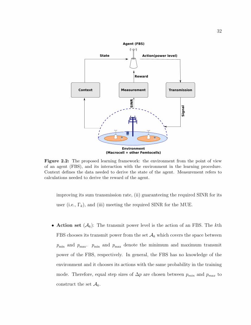
Figure 2.2: The proposed learning framework: the environment from the point of viewof an agent (FBS), and its interaction with the environment in the learning procedure.Context defines the data needed to derive the state of the agent. Measurement refers tocalculations needed to derive the reward of the agent.
improving its sum transmission rate, (ii) guaranteeing the required SINR for its
user (i.e., Γk), and (iii) meeting the required SINR for the MUE.
• Action set (Ak): The transmit power level is the action of an FBS. The kth
FBS chooses its transmit power from the set Ak which covers the space between
pmin and pmax. pmin and pmax denote the minimum and maximum transmit
power of the FBS, respectively. In general, the FBS has no knowledge of the
environment and it chooses its actions with the same probability in the training
mode. Therefore, equal step sizes of ∆p are chosen between pmin and pmax to
construct the set Ak.

33
• State set (Xk): State set directly affects the performance of the MUE and the
FUEs. To this end, we define four variables to represent the state of the network.
The state set variables are defined based on the constraints of the optimization
problem in (2.3). We define the variables X1 and X2 as indicators of the
performance of the FUE and the MUE. On the other hand, the relative location
of an FBS with respect to the MUE and the MBS is important and affects the
interference power at the MUE caused by the FBS, and the interference power
at the FBS causes by the MBS. Therefore, we define X3 as an indicator of
the interference imposed on the MUE by the FBS, and X4 as an indicator
of interference imposed on the femtocell by the MBS. The state variables are
defined as
– X1 ∈ 0, 1: The value of X1 indicates whether the FBS is supporting
its FUE with the required minimum SINR or not. X1 is defined as X1 =
1γk≥Γk.
– X2 ∈ 0, 1: The value of X2 indicates whether the MUE is being sup-
ported with its required minimum SINR or not. X2 is defined as X2 =
1γ0≥Γ0.
– X3 ∈ 0, 1, 2, ..., N1: The value of X3 defines the location of the FBS
compared to N1 concentric rings around the MUE. The radius of rings are
d1, d2, ..., dN1 .
– X4 ∈ 0, 1, 2, ..., N2: The value of X4 defines the location of the FBS
compared to N2 concentric rings around the MBS. The radius of rings are
d′1, d′2, ..., d′N2.

34
The kth FBS calculates γk based on the channel equality indicator (CQI)
received from its related FUE to assess X1. The MBS is aware of the SINR
of the MUE user, i.e., γ0, and the relative location of the FBS concerning itself
and the MUE. Therefore, the FBS obtains the required information to asses the
X2, X3, and X4 variables via backhaul and feedback from the MBS.
Here, we defined the state variables as a function of each FBS’s SINR and
location. Therefore, in high SINR regime, the state of FBSs can be assumed to
be independent of each other.
In Section 3.6, we will examine different possible state sets to investigate the
effect of the above state variables on the performance of the network.
2.5 Q-DPA, Reward Function, and Sample Complexity
In this section, we present Q-DPA, which is an application of the proposed framework.
Q-DPA details the learning method, the learning rate, and the training procedure.
Then, the proposed reward function is defined. Finally, the required sample complex-
ity for the training is derived.
2.5.1 Q-learning Based Distributed Power Allocation (Q-DPA)
To solve the Bellman equation in (2.6), we use Q-learning. The reasoning for choosing
the RL method and advantages of Q-learning are explained in Sections 2.4.1 and 2.1.1,
respectively. The Q-learning update rule to evaluate a policy for the global Q-function
can be represented as (2.12)

35
Q(x(t), a(t))←Q(x(t), a(t))+
α(t) (x, a)
R(t+1)(x(t), a(t)
)+ βmax
a′Q(x(t+1), a′)︸ ︷︷ ︸
(M)
−Q(x(t), a(t))
,
(2.12)
where a′ ∈ A, α(t) (x, a) denotes the learning rate at time step t, and x(t+1) is the new
state of the network [25]. The term M is the maximum value of the global Q-function
that is available at the new state x(t+1). After each iteration, the FBSs will receive
the delayed reward R(t+1)(x(t), a(t)
)and then the global Q-function will be updated
according to (2.12).
In the prior works [46–48,50,51], a constant learning rate was used for Q-learning
to solve the required optimization problems. However, according to [64], in finite
number of iterations, the performance of Q-learning can be improved by applying a
decaying learning rate. Therefore, we use the following learning rate
α(t) (x, a) =1
[1 + t (x, a)], (2.13)
in which t (x, a) refers to the number of times, until time step t, that the state-action
pair (x, a) is visited. It is worth mentioning that, by using the above learning rate,
we need to keep track of the number of times each state-action pair has been visited
during training, which requires more memory. Therefore, at the cost of more memory,
a better performance can be achieved.
There are two alternatives available for the training of new FBSs as they join the
network, they can use independent learning or cooperative learning. In independent
learning, each FBS tries to maximize its own Q-function. In other words, using the
factorization method in Section 2.4.2, the term M in (2.12) is approximated as

36
M = maxa′
∑k∈K
Qk(x(t+1)k , a′k) ≈
∑k∈K
maxa′k
Qk
(x
(t+1)k , a′k
). (2.14)
In cooperative learning, the FBSs share their local Q-functions and will assume
that the FBSs with the same state make the same decision. Hence, term M is
approximated as
M = maxa′
∑k∈K
Qk(x(t+1)k , a′k) ≈ max
a′k
∑k∈K′
Qk
(x
(t+1)k , a′k
), (2.15)
where K′ is the set of FBSs with the same state x(t+1)k . Cooperative Q-learning may
result in a higher cumulative reward [65]. However, cooperation will result in the same
policy for FBSs with the same state and additional overhead since the Q-functions
between FBSs need to be shared over the backhaul network. The local update rule
for the kth FBS can be derived from (2.12) as in (2.16)
Qk(x(t)k , a
(t)k )←Qk(x
(t)k , a
(t)k )+
α(t)(R(t+1)
(x
(t)k , a
(t)k
)+ βQk
(x
(t+1)k , a∗k
)−Qk(x
(t)k , a
(t)k )),
(2.16)
where, R(t+1)(x
(t)k , a
(t)k
)is the reward of the kth FBS, and a∗k is defined as
arg maxa′k
Qk
(x
(t+1)k , a′k
), (2.17)
and
arg maxa′k
∑k∈K′
Qk
(x
(t+1)k , a′k
), (2.18)
for independent and cooperative learning, respectively.

37
In this paper, a tabular representation is used for the Q-function in which the
rows of the table refer to the states and the columns refer to the actions of an agent.
Generally, for large state spaces, neural networks are more efficient to use as Q-
functions, however, part of this work is focused on the effect of state space variables.
Therefore, we avoid large number of state variables. On the other hand, we provide
exhaustive search solution to investigate the optimality of our solution which is not
possible for large state spaces.
The training for an FBS happens over L frames. In the beginning of each frame,
the FBS chooses an action, i.e., transmit power. Then, the FBS sends a frame to the
intended FUE. The FUE feeds back the required measurements such as CQI so the
FBS can estimate the SINR at the FUE, and calculate the reward based on (2.24).
Finally, the FBS updates its Q-table according to (2.16).
Due to limited number of training frames, each FBS needs to select its actions
in a way that covers most of the action space and improves the policy at the same
time. Therefore, the FBS chooses the actions with a combination of exploration and
exploitation, known as an e-greedy exploration. In the e-greedy method, the FBS acts
greedily with probability 1− e (i.e., exploiting) and randomly with probability e (i.e.,
exploring). In exploitation, the FBS selects an action that has the maximum value
in the current state in its own Q-table (independent learning) or in the summation
of Q-tables (cooperative learning). In exploring, the FBS selects an action randomly
to cover action space and avoid biasing to a local maximum. In [2], it is shown that
for a limited number of iterations the e-greedy policy results in a closer final value to
the optimal value compared to only exploiting or exploring.
It is worth mentioning that the overhead of sharing Q-tables depends on the
definition of the state model Xk according to Section 2.4.3. For instance, assuming

38
the largest possible state model as Xk = X1, X2, X3, X4. The variables X3 and
X4 depend on the location of the FBS and are fixed during training. Therefore, one
training FBS uses four rows of its Q-table and just needs the same rows from other
FBSs. Hence, if the number of active FBSs is |K|, the number of messages to the
FBS in each training frame is 4× (|K| − 1), each of size |Ak|.
2.5.2 Proposed Reward Function
The design of the reward function is essential because it directly impacts the objectives
of the FBS. Generally, there has not existed a quantitative approach to designing the
reward function. Here, we present a systematic approach for deriving the reward
function based on the nature of the optimization problem under consideration. Then,
we compare the behavior of the designed reward function to the ones in [46–48].
The reward function for the kth FBS is represented as Rk. According to the
Section 2.4.3, the kth FBS has knowledge of the minimum required SINR for the
MUE, i.e. Γ0, and minimum required SINR for its related FUE, i.e. Γk. Also, after
taking an action in each step, the kth FBS has access to the rate of the MUE, i.e. r0
and the rate of its related FUE, i.e. rk. Therefore, Rk is considered as a function of
the above four variables as Rk : (r0, rk,Γ0,Γk)→ R.
In order to design the appropriate reward function, we need to estimate the
progress of the kth FBS toward the goals of the optimization problem. Based on
the input arguments to the reward function, we define two progress estimators, one
for the MUE as (r0 − log2 (1 + Γ0)) and one for the kth FUE as (rk − log2 (1 + Γk)).
To reduce computational complexity, we define the reward function as a polynomial
function of the defined progress estimators as

39
Rk = (r0 − log2 (1 + Γ0))k1 + (rk − log2 (1 + Γk))k2 + C, (2.19)
where, k1 and k2 are integers and C ∈ R is a constant referred to as the bias of the
reward function.
The constant bias, C, in the reward function has two effects on the learning
algorithm: (i) The final value of the states for a given policy π, and (ii) the behavior
of the agent in the beginning of the learning process as follows:
1. Effect of bias on the final value of the states: Assume the reward function,
R1 = f (·), and the reward function R2 = f (·) +C, C ∈ R. We define the value
of state x for a given policy π using R1 as V1 (x) and the value of the state x
for the same policy using R2 as V2 (x). According to (2.4), we have
V2 (x) = Eπ
[∞∑t=0
βt(f (t+1) (·) + C
)]
= Eπ
[∞∑t=0
βtf (t+1) (·)
]+ C
∞∑t=0
βt
= V1 (x) +C
1− β.
(2.20)
Therefore, bias of the reward function adds the constant value C1−β to the value
of the states. However, all the states are affected the same after the convergence
of the algorithm.
2. Effect of bias in the beginning of the learning process: This effect is studied
using the action-value function of an agent, i.e., the Q-function. Assume that
the Q-function of the agent is initialized with zero values and the reward function
is defined as R = f (·) + C. Further let us consider the first transition of the

40
agent from state x′ to state x′′ happens by taking action a at time step t, i.e.,
x(t) = x′ and x(t+1) = x′′. The update rule at time step t is given by (2.16) as
in (2.21)
Q(x′, a)← Q(x′, a) + α(t) (x′, a)(R (x′, a) + β max
a′Q (x′′, a′)−Q(x′, a)
)← α(t) (x′, a)
(f (·) + β max
a′Q (x′′, a′)
)+ α(t) (x′, a)C︸ ︷︷ ︸
(A)
.
(2.21)
According to the above, after the first transition from the state x′ to the state
x′′, the Q-value for the state x′ is biased by the term (A). If (A > 0), the value
of the state x′ increases and if (A < 0), the value of the state x′ decreases.
Therefore, the already visited states will be more or less attractive to the agent
in the beginning of the learning process as long as the agent has not explored
the state-space enough.
The change of behavior of the agent in the learning process can be used to bias the
agent towards the desired actions or states. However, in basic Q-learning the agent
has no knowledge in prior about the environment. Therefore, we select the bias equal
to zero, C = 0, and define the reward function as follows.
Definition 2. The reward function for the kth FBS, Rk : (r0, rk,Γ0,Γk) → R, is a
continuous and differentiable function on R2 defined as (2.22)
Rk (r0, rk,Γ0,Γk) = (r0 − log2 (1 + Γ0))k1 + (rk − log2 (1 + Γk))k2 , (2.22)
where k1 and k2 are integers.

41
The objective of the FBS is to maximize its transmission rate. On the other hand,
high transmission rate for the MUE is a priority for the FBS. Therefore, Rk should
have the following property
∂Rk
∂ri≥ 0, i = 0, k. (2.23)
The above property implies that higher transmission rate for the FBS or the MUE
results in higher reward. Hence, considering Definition 2, we design a reward function
that motivates the FBSs to increase rk and r0 as much as possible even more than
the required rate as follow
Rk = (r0 − log2 (1 + Γ0))2m−1 + (rk − log2 (1 + Γk))2m−1 , (2.24)
wherem is an integer. The above reward function considers the minimum rate require-
ments of the FUE and the MUE, while encourages the FBS to increase transmission
rate of both.
To further understand the proposed reward function, we discuss reward functions
that are used by [46–48]. We refer to the designed reward function in [46] as quadratic,
in [47] as exponential, and in [48] as proximity reward functions. The quadratic reward
function is designed based on a conservative approach. In fact, the FBS is enforced
to select actions that result in transmission rate close to the minimum requirement.
Therefore, higher or lower rate than the minimum requirement results in a same
amount of reward. The behavior of the quadratic reward function can be explained
as follow

42
∂Rk
∂ri× (ri − log2 (1 + Γi)) ≤ 0, i = 0, k. (2.25)
The above property implies that if the rate of the FBS or the MUE is higher than the
minimum requirement, the actions that increase the rate will decrease the reward.
Hence, this property is against increasing sum transmission rate of the network. The
exponential and proximity reward functions have the property in (2.23) for the rate
of the FBS, and the property in (2.25) for the rate of the MUE. In another words,
they satisfy the following properties
∂Rk
∂r0
× (r0 − log2 (1 + Γ0)) ≤ 0,
∂Rk
∂rk≥ 0.
(2.26)
As the density of the FBSs increases, the above properties result in increasing transmit
power to achieve higher individual rate for a FUE while introducing higher interfer-
ence for the MUE and other neighbor FUEs. In fact, as increasing the FUE rate is
rewarded, taking actions that result in increasing the MUE rate decreases the reward.
However, the FBS should have the option of decreasing its transmit power to increase
the rate of the MUE. This behavior is important since it causes an FBS to produce
less interference for its neighboring femtocells. Therefore, we give equal opportunity
for increasing the rate of the MUE or the FUE.
The value of reward functions for different FBSs is different, however they have the
same behavior. Here, we plot the value of the four reward functions that are discussed
above. The plots refers to the proposed (Fig. 2.3(a)), quadratic (Fig. 2.3(b)), expo-
nential (Fig. 2.3(c)), and proximity (Fig. 2.3(d)) reward functions. The important
information that can be obtained from these plots are the maximal points of the

43
(a) (b)
(c) (d)
Figure 2.3: Reward functions: (a) Proposed reward function with m = 2, (b) Quadraticreward function with zero maximum at (4.0, 0.5), (c) Exponential reward function, (d)Proximity reward function.
reward functions, behavior of the reward functions around minimum requirements,
and behavior of the reward functions by increasing rk or r0. The proposed reward
function in Fig. 2.3(a) shows pushing the FBS to select transmit power levels that
increase both rk and r0, while other reward functions have their maximum around
the minimum rate requirements.
44
2.5.3 Sample Complexity
In each training frame, Q-DPA collects one sample from the environment represented
as the state-action pair in the Q-function. Sample complexity is defined as the
minimum number of samples that is required to train the Q-function to achieve an
ε-optimal policy. For ε > 0 and δ ∈ (0, 1], π is an ε-optimal policy if [66]
Pr (‖Q∗ −Qπ‖ < ε) ≥ 1− δ. (2.27)
The sample complexity depends on the exploration policy that is generating the
samples. In Q-DPA, e-greedy policy is used as the exploration policy. However,
e-greedy policy depends on the Q-function of the agent which is being updated. In
fact, the distribution of e-greedy policy is unknown. Here, we provide a general bound
on the sample complexity of Q-learning.
Proposition 1. Assume Rmax is the maximum of the reward function for an agent
and Q(T ) is the action-value for state-action pair (x, a) after T iterations. Then, with
probability at least 1− δ, we have
‖Q∗ −Q(T )‖ ≤ 2Rmax
(1− β)
[β
T (1− β)+
√2
Tln
2|X |.|A|δ
]. (2.28)
Proof. See Appendix A.1.
This proposition proves the stability of Q-learning and helps us to provide a
minimum number of iterations to achieve ε > 0 error with respect to Q∗ with
probability 1− δ for each state-action pair. By assuming the right term of the above
inequality as ε, the following Corollary is concluded.

45
defabc
mnojkl
wxyztuvpqrs
ghi
@
* + 0
87
4
1 2
5
9
6
3
www . ABC - color . com
defabc
mnojkl
wxyztuvpqrs
ghi
@
* + 0
87
4
1 2
5
9
6
3
www . ABC - color . com
defabc
mnojkl
wxyztuvpqrs
ghi
@
* + 0
87
4
1 2
5
9
6
3
www . ABC - color . com
defabc
mnojkl
wxyztuvpqrs
ghi
@
* + 0
87
4
1 2
5
9
6
3
www . ABC - color . com
defabc
mnojkl
wxyztuvpqrs
ghi
@
* + 0
87
4
1 2
5
9
6
3
www . ABC - color . com
defabc
mnojkl
wxyztuvpqrs
ghi
@
* + 0
87
4
1 2
5
9
6
3
www . ABC - color . com
defabc
mnojkl
wxyztuvpqrs
ghi
@
* + 0
87
4
1 2
5
9
6
3
www . ABC - color . com
defabc
mnojkl
wxyztuvpqrs
ghi
@
* + 0
87
4
1 2
5
9
6
3
www . ABC - color . com
defabc
mnojkl
wxyztuvpqrs
ghi
@
* + 0
87
4
1 2
5
9
6
3
www . ABC - color . com
defabc
mnojkl
wxyztuvpqrs
ghi
@
* + 0
87
4
1 2
5
9
6
3
www . ABC - color . com
FBS
FUE
MUE
10m
10m
10m
10m
Figure 2.4: Dense urban scenario with a dual strip apartment block located at distanceof 350 m of the MBS; FUEs are randomly located inside each apartment.
Corollary 1. For any ε > 0, after
T = Ω
(8R2
max
ε2 (1− β)2 ln2|X |.|Ak|
δ
)(2.29)
number of iterations, Q(T ) reaches ε-optimality with probability at least 1− δ.
2.6 Simulation Results
The objective of this section is to validate the performance of the Q-DPA algorithm
with different learning configurations in a dense urban scenario. We first introduce
the simulation setup and parameters. Then, we introduce four different learning
configurations and we analyze the trade-offs between them. Finally, we investigate the
performance of the Q-DPA with different reward functions introduced in Section 2.5.2.
For the sake of simplicity, we use the notation IL as independent learning and CL as
cooperative learning.

46
Table 2.1: Urban dual strip pathloss model
Link PL(dB)
MBS to MUE 15.3 + 37.6 log10R ,
MBS to FUE 15.3 + 37.6 log10R+ Low ,
FBS to FUE (same apt strip) 56.76 + 20 log10R+ 0.7d2D,indoor ,
FBS to FUE (different apt strip) max(15.3 + 37.6 log10R,38.46 + 20 log10R) + 18.3 + 0.7d2D,indoor + Low.
Table 2.2: Simulation Parameters
parameters Value parameters Value
Frame time 2 ms d′1, d′2, d′3 50, 150, 400 m
Thermal noise -174 dBm/Hz d1, d2, d3 17.5, 22.5, 45 mTraffic model Fullbuffer
Q-DPA parameters Value parameters Value
Training period (iterations) L T × |X |.|Ak| pmin 5 dBmLearning parameter β 0.9 pmax 15 dBmExploratory probability (e) 10% ∆p 1 dBm
2.6.1 Simulation Setup
We use a dense urban scenario as the setup of the simulation as illustrated in Fig. 2.4.
We consider one macrocell with radius 350 m which supports multiple MUEs. The
MBS assigns a subband to each MUE. Each MUE is located within a block of
apartments and each block contains two strip of apartments. Each strip has five
apartments of size 10 m×10 m. There is one FBS located in the middle of each
apartment which supports an FUE within a 5 m distance. We assume that the FUEs
are always inside the apartments. The FBSs are closed-access, therefore, the MUE
is not able to connect to any FBS, however, it receives interference from the FBSs
working on the same subband as itself.
Here, we assume that the MUE and all the FBSs work on the same sub-carriers to

47
consider the worst case scenario (high interference scenario). However, the extension
of the simulation to the multi-carrier scenario is straight forward but does not affect
our investigations. We assume the block of apartments is located on the edge of the
macrocell, i.e., 350 m distance from the MBS, and the MUE is assumed to be in
between the two strip of apartments.
In these simulations, in order to initiate the state variables X3 and X4 in Sec-
tion 2.4.3, the number of rings around the MBS and the MUE are assumed to be
three (N1 = N2 = 3). Although, as the density increases, more rings with smaller
diameters can be used to more clearly distinguish between the FBSs.
It is assumed that the FBSs and the MBS operate at f = 2.0 GHz. The MBS
allocates 33 dBm as its transmit power, and the FBSs choose their transmit power
from a range of 5 dBm to 15 dBm with power steps of 1 dB. In order to model
the pathloss, we use the urban dual strip model from 3GPP TR 36.814 [67]. The
pathloss model of different links are provided in Table 2.1. In Table 2.1, R is the
distance between a transmitter and a receiver in meters, Low is the wall penetration
loss which is set to 20 dB [67]. d2D,indoor is the 2-dimensional distance. We assume
that the apartments are single floor, therefore, d2D,indoor ≈ R. The fourth row of the
pathloss models is used for the links between the FBSs and the MUE.
The minimum SINR requirements for the MUE and the FUEs are defined based
on the required rate needed to support their corresponding user. In our simulations,
the minimum required transmission rate to meet the QoS of the MUE is assumed to
be 4 (b/s/Hz), i.e., log2(1 + Γ0) = 4 (b/s/Hz). Moreover, for the FUEs the minimum
required rate is set to 0.5 (b/s/Hz), i.e, log2(1 + Γk) = 0.5 (b/s/Hz), k ∈ K. It is
worth mentioning that by knowing the media access control (MAC) layer parameters,
the values of the required rates can be calculated using [68, Eqs. (20) and (21)].
48
To perform Q-learning, the minimum number of required frames, i.e., L, is calcu-
lated based on achieving 90% optimality, with probability of at least 0.9, i.e., δ = 0.1.
The simulation parameters are given in Table 2.2. The value of the Q-learning
parameters are selected according to our simulations and references [46–51].
The simulation starts with one femtocell. The FBS starts running Q-DPA in
Section 2.5.1 using IL. After convergence, the next FBS is added to the network.
The new FBS runs Q-DPA, while the other FBS is already trained, and will just
act greedy to choose its transmit power. After convergence of the second FBS, the
next one is added to the network, and so on. We represent all the results versus
the number of active femtocells in the system, from one to ten. Considering the size
of the apartment block, and the assumption that all femtocells operate on the same
frequency range, the density of deployment varies approximately from 600 FBS/km2
to 6000 FBS/km2.
2.6.2 Performance of Q-DPA
Here, we show the simulation results of distributed power allocation with Q-DPA.
First, we define two different state sets. The sets are defined as X1 = X1, X3, X4
and X2 = X2, X3, X4. In both sets, FBSs are aware of their relative location to the
MUE and the MBS due to the presence of X3 and X4, respectively. The state set X1
gives knowledge of the status of the FUE to the FBS, and the state set X2 provides
knowledge of the status of the MUE to the FBS.
In order to understand the effect of independent and cooperative learning, and
the effect of different state sets, we use four different learning configurations as:
independent learning with each of the two state sets as IL+X1 and IL+X2, and
cooperative learning with each of the two state sets as CL+X1 and CL+X2. The

49
2 4 6 8 10
FBS Numbers
3
4
5
6
7
8
9
10M
UE
tra
nsm
issio
n r
ate
(b/s
/Hz)
(a)
2 4 6 8 10
FBS Numbers
0
5
10
15
20
Sum
tra
nsm
issio
n r
ate
(b/s
/Hz)
(b)
2 4 6 8 10
FBS Numbers
50
100
150
200
250
300
350
Sum
pow
er
(mW
att)
(c)
Figure 2.5: Performance of different learning configurations: (a) transmission rate of theMUE, (b) sum transmission rate of the FUEs, (c) sum transmit power of the FBSs.
results are compared with greedy approach in which each FBS chooses maximum
transmit power. The simulation results are shown in three figures as: transmission
rate of the MUE (Fig. 2.5(a)), sum transmission rate of the FUEs (Fig. 2.5(b)), and
sum transmit power of the FBSs (Fig. 2.5(c)).
According to Fig. 2.5(c), in the greedy algorithm, each FBS uses the maximum
available power for transmission. Therefore, the greedy method introduces maximum
interference for the MUE and has the lowest MUE transmission rate in Fig. 2.5(a).

50
On the other hand, despite using maximum power, the greedy algorithm does not
achieve highest transmission rate for the FUEs either (Fig. 2.5(b)). This is again due
to the high level of interference.
The state set X2 provides knowledge of MUE’s QoS status to the learning FBSs.
Therefore, as we see in Fig. 2.5(a), the performance of IL with X2 is higher than the
ones with X1. This statement is true for CL too. We can see the reverse of this
conclusion in the FUEs’ sum transmission rate in Fig. 2.5(b). The performance of
IL with X1 is higher than IL with X2. This is because the FBSs are aware of the
status of the FUE, therefore, they consider actions that result in the state variable
X1 = 1γk≥Γk to be 1. This is true in comparison of the states in CL too. In
conclusion, the state set X1 works in favor of femtocells and the state set X2 benefits
the MUE.
We conclude from the simulation results that IL and CL present different trade-
offs. More specifically, IL supports a higher sum transmission rate for the FBSs and
a lower transmission rate for the MUE, while CL can support a higher transmission
rate for the MUE at the cost of an overall lower sum transmission rate for the FBSs.
From a power consumption point of view, IL results in a higher power consumption
when compared to that of CL. In general, IL trains an FBS to be selfish compared
to CL. IL can be very useful when there is no means of communication between the
agents. On the other hand, CL trains an FBS to be more considerate about other
FBSs at the cost of communication overhead.
In Table 2.3, we have compared the performance of the four learning configura-
tions. In each column, number 1 is used as a metric to refer to the highest performance
achieved and number 4 is used to refer to the lowest performance observed. The first
column represents the summation of transmit powers of FBSs, the second column

51
Table 2.3: Performance of different learning configurations. 1 is the best, and 4 is theworst.
Learning configuration∑pk
∑rk r0
IL+X1 4 1 4
CL+X1 3 3 3
IL+X2 2 2 2
CL+X2 1 4 1
indicates the summation of transmission rates of the FUEs, and the third column
denotes the transmission rate of the MUE.
2.6.3 Reward Function Performance
Here, we compare the performance of the four reward functions discussed in Sec-
tion 2.5.2. Since the objective is to maximize the sum transmission rate of the
FUEs, according to Table 2.3, we choose the combination IL+X1 as the learning
configuration. The performance of the reward functions are provided as the MUE
transmission rate (Fig. 2.6(a)), sum transmission rate of the FUEs (Fig. 2.6(b)), and
sum transmission power of the FBSs (Fig. 2.6(c)). In each figure, the solution of the
optimization problem with exhaustive search and the performance of greedy method
are provided. The exhaustive search provides us with the highest achievable sum
transmission rate for the network. The quadratic, exponential, and proximity reward
functions result in fast decaying of MUE transmission rate, while the proposed reward
function results in a much slower decrease of the rate for the MUE. The proposed
reward function manages to achieve a higher sum transmission rate compared to that
of the other three reward functions as well. Fig. 2.6(c) indicates that the proposed
reward function reduces the sum transmitted power at the FBSs which in turn could

52
2 4 6 8 10
FBS Numbers
3
4
5
6
7
8
9
10
11
12M
UE
tra
nsm
issio
n r
ate
(b/s
/Hz)
(a)
2 4 6 8 10
FBS Numbers
0
5
10
15
20
Su
m t
ran
sm
issio
n r
ate
(b
/s/H
z)
(b)
2 4 6 8 10
FBS Numbers
50
100
150
200
250
300
350
Sum
tra
nsm
it p
ow
er
(mW
att)
(c)
Figure 2.6: Performance of the proposed reward function compared to quadratic, exponen-tial and proximity reward functions: (a) transmission rate of the MUE, (b) sum transmissionrate of the FUEs, (c) sum transmit power of the FBSs.
result in lower levels of interference at the FUEs. In comparison with the exhaustive
search solution as the optimal solution, there is a gap of performance. For instance
according to Fig. 2.6(c), for eight number of FBSs, the proposed reward function uses
an average of 50 mWatt less sum transmit power than the optimal solution. However,
as we see in Fig. 2.6(b) and Fig. 2.6(a), by using more power, the sum transmission
rate can be improved and the transmission rate of the MUE can be decreased to
the level of exhaustive solution without violating its minimum required rate. In our

53
future works, we wish to cover this gap by using neural networks as the function
approximator of the learning method.
2.7 Conclusion
In this chapter, we proposed a learning framework for a two-tier femtocell network.
The framework enables addition of a new femtocell to the network, while the femtocell
trains itself to adapt its transmit power to support its serving user while protecting
the macrocell user. On the other hand, the proposed method as a distributed
approach can solve the power optimization problem in dense HetNets, while sig-
nificantly reducing power usage. The proposed framework is generic and motivates
the design of machine learning based SONs for management schemes in femtocell
networks. Besides, the framework can be used as a bench test for evaluating the
performance of different learning configurations such as Markov state models, reward
functions and learning rates. Further, the proposed framework can be applied to
other interference-limited networks such as cognitive radio networks as well.

54
Chapter 3
POWER ALLOCATION IN INTERFERENCE-LIMITED
NETWORKS VIA COORDINATED LEARNING
In Chapter 2, we focused on transmit power control in a two-tier HetNet and modeled
the whole network as a single Markov decision problem (MDP). With introduction of
independent and cooperative learning, the MDP was factorized into local Q-functions.
However, there was a performance gap between the independent/cooperative learning
and the exhaustive search. In this chapter, we focus on transmit power control in
an interference-limited network of small base stations (SBSs). We follow the same
procedure and define a global Q-function relating to the whole network. However, in
order to fill the performance gap, we feed the interference model of the network to the
factorization process. In fact, we investigate the effect of accurate MDP factorization
on the optimality of the solution. The proposed method leverages coordination
through simple message passing between SBSs to achieve an optimal joint power
allocation. Simulation results show the optimality of the proposed method for a
two-user case. This work was published in [28].

55
3.1 Introduction
Supporting the expected cellular traffic growth is one of the main tasks for the next
generation (a.k.a “5G”) wireless cellular networks and densification is one of the
main technologies to achieve such growth [3]. A key driver for densification will
be deployment of small base stations (SBSs) [69]. The SBSs might be mounted by
users in a plug-and-play fashion, and their backhaul may be supported by broadband
connections. The user-mounted feature, introduces unplanned deployment of SBSs,
which may result in unavoidable co-channel interference. In a dense network, in
which the architecture of the network changes sporadically, a self-organizing method
is a viable solution to manage the network resources.
One of the requirements of algorithms designed for self-organizing networks (SONs)
is working under open loop communication conditions. This means transmitter has
access to the signal-to-interference-plus-noise ratio (SINR) values while does not have
access to the channel state information (CSI). In fact, radio measurements such as
SINR, are part of the Big data in cellular networks [36]. In this regard, one of the
main advantages of multi-agent reinforcement learning (MARL) solutions is to utilize
the measured SINR values. Generally most of the classic optimization solutions are
based on channel coefficients. Thus, the prior methods require full CSI to find the
solution while the MARL methods only need access to existing radio measurements,
i.e., the measured SINR values. To this end, cooperative MARL methods have been
used in resource management of communication networks [27, 70–72]. However, the
existing MARL approaches in communication network management do not address
the optimality of their cooperation methods. This is an important research topic to
address since finding the optimal joint power allocation is directly impacted by the

56
nature of the cooperation approach. In this chapter, we focus on an interference-
limited network. We propose a factorization method to achieve optimal solution in
transmit power control to maximize sum transmission rate of the system.
3.1.1 Related Work
The problem of power allocation in an interference-limited network has been inves-
tigated widely in the literature. In [73] and [74], the optimal power allocation for
a two-user interference channel is derived for sum and individual power constraints,
respectively. In [75] a more general solution is proposed for multi-transmitter systems
with individual power constraints. The solution depends on the SINR value. In high
SINR regime, the optimal solution is derived through transforming the problem into
a geometric programming (GP) problem, while in the low SINR regime, a heuristic
solution based on solving multiple GPs is used. It is important to note that all of
these prior approaches are based on interior point methods. Hence, they require a
centralized network management approach which may be impossible in dense net-
works. In [75], a distributed method based on decomposing the optimization problem
into local problems is proposed. The solution is based on message-passing and applies
to high SINR case with full CSI. Nonetheless, in a dense plug-and-play network, with
a changing architecture, the assumptions of high SINR and the availability of full CSI
at all nodes may not hold.
3.1.2 Contributions
In this chapter, we find an optimal joint power allocation solution via coordination be-
tween deployed SBSs. To address the optimality of the MARL approach, we model the
whole system as a Markov decision process (MDP) with the SBSs being represented

57
as the agents of the MDP. Then, we define a coordination graph according to the
interference model of the network. Subsequently, MDP is factorized to local ones and
the value function of the MDP is approximated by a linear combination of local value
functions. As we mentioned before, in order to remove the need for access to CSI, and
develop an adaptable algorithm that handles a changing network architecture, each
SBS uses a model-free reinforcement learning approach, i.e., Q-learning. Q-learning
is used to update the SBS’s local value function. Subsequently, we leverage the
ability of SBSs to communicate over the backhaul network to build a simple message
passing structure to select a transmit power action based on the variable elimination
method. Finally, we propose a distributed algorithm which finds an optimal joint
power allocation to maximize the sum transmission rate.
This chapter is organized as follows. In Section 5.2, the system model is presented.
Section 3.3 first introduces the optimization problem, then analyzes the convexity of
the problem. Section 3.4 presents the general framework of the proposed solution.
Section 3.5 outlines the proposed power allocation scheme while Section 3.6 presents
simulation results. Finally, Section 3.7 concludes the chapter.
3.2 System Model
We consider downlink transmission in a dense deployment of N SBSs. We assumed
each SBS supports one user equipment (UE), and all SBSs share the same frequency
resource block. This system can represent a single cluster of a large network, which
uses different frequency in each cluster to avoid interference between clusters. It
is also assumed the SBSs are interconnected via a backhaul network supported by,
for example, a broadband connection. Here, we use the same model of interference

58
as [73]. Thus, the received signal at the ith UE, ri is given by
ri =√giPidi +
∑j∈Di
√giPjβjidj + ni, (3.1)
where gi represents the channel gain between the ith SBS and the UE it is serving,
di is the transmitted signal from the ith SBS, Pi is the transmitted power at the
ith SBS, Di represents the set of interfering SBSs to the ith UE, βji (0 ≤ βji ≤ 1)
for 1 ≤ i ≤ N and j ∈ Di is the ratio of the unintended power of the jth SBS
when measured at the ith UE, and ni is the zero mean additive white Gaussian noise
(AWGN) at the ith UE with variance σ2. According to the signal representation in
(3.1), the SINR at the ith UE, SINRi, can be determined as
SINRi =giPi∑
j∈DigiPjβji + σ2
, (3.2)
and the throughput at the ith UE normalized by the transmission bandwidth, Ri, is
calculated as
Ri = log2 (1 + SINRi) . (3.3)
It is worth noting that the proposed solution will use the measured SINR, and does
not need to estimate the values of channel gains.
3.3 Problem Analysis
Let us define P = P1, P2, ..., PN as the set containing the transmitted power of
the SBSs. The goal of the optimization is to find the optimal joint power allocation
59
between SBSs, P∗ = P ∗1 , P ∗2 , ..., P ∗N, that maximizes the total throughput of the
network. The optimization problem (OP1) can be formulated as
maximizeP
N∑i=1
Ri =N∑i=1
log2 (1 + SINRi) , (3.4a)
subject to Pi ≤ Pi,max, i = 1, . . . , N. (3.4b)
Here, the objective function in (3.4a) maximizes the sum throughput of the network.
The constraint (3.4b) refers to the individual power limitation of every SBS.
3.3.1 Problem Analysis
The optimization problem (OP1) is a non-convex optimization problem. Here, first we
will investigate the non-convexity of OP1, and then we will examine the approximate
solutions to the problem in two regimes : (1) high SINR, and low to medium SINR.
Non-Convexity of OP1
The objective function in (3.4a) contains the interference term in the denominator of
SINR term. In a dense network the interference term cannot be ignored [59]. Due to
the presence of the interference term, the objective function (3.4a) is a non-concave
function [58], which leads to non-convexity of the optimization problem.
Approximate Problems
• High SINR : If the condition SINR 1 holds, which means signal level is
much higher than the interference level, the objective function in OP1 can be
approximated as

60
N∑i=1
log2 (1 + SINRi) =N∑i=1
log2(SINRi) = log2(N∏i=1
SINRi). (3.5)
By using the above approximation, and representing the objective function and
the constraints using posynomials, OP1 can be represented in the form of geo-
metric programming (GP) problem. GP is a nonlinear, nonconvex optimization
problem which can be transformed into a convex optimization problem and can
be solved in efficient time [75].
• Low to medium SINR : If the SINR value is not much larger than 0dB, the
approximation in (3.5) does not hold. Although by using the posynomial
format, 1 + SINRi can be represented as a ratio of two posynomials. In this
format, the optimization problem falls into a nonconvex class of problems called
Complementary GP [75]. The Complementary GP problems are intractable
NP-hard problems.
As we mentioned before, in both of the above cases, the solutions are based on the
availability of CSI at the transmitters (SBSs). However, the assumption of open-loop
communication which is one of the features of SONs disqualifies availability of CSI at
the transmitter. Hence, SBSs need to select their transmit power just based on the
measured SINR fed back from their assigned users.
3.3.2 Nash Equilibrium and Pareto Optimality
Since the goal of the optimization problem is to maximize the sum throughput of the
network, OP1 can be viewed as a fully cooperative game. A fundamental solution to
a game is the Nash equilibrium [76]. The Nash equilibrium is a joint action in a game,
where deviating from this action when considering the actions of other agents is not
61
profitable to the agent taking the action. Any game can have multiple solutions for
the Nash equilibrium. Another concept is the Pareto optimality of a solution. A joint
action is Pareto optimal, if an agent can not gain more performance without reducing
the performance of at least one other agent in the game. In a fully cooperative game,
each Pareto optimal solution is a Nash equilibrium, which can be achieved using
coordination between agents [77].
3.4 Distributed Coordinated Q-learning
In this section, the proposed optimal solution based on the Markov decision process
(MDP) is presented. Then, the dimensionality issues of the optimal solution will
be investigated. The dimensionality is important since it affects the tractability of
the problem. Next, we use the coordination method introduced by [78] to solve the
problem in a distributed fashion. We show that the resulting method, provides a joint
solution for the MDP via message passing between the agents of the network.
3.4.1 Optimal Solution via Q-learning
Consider a system with N agents, where each agent j selects its actions from its action
set, Aj. Further, X = X1, X2, ..., Xn is the set of state variables which define the
state of the system. Let us denote x ⊂ X to represent a single state of the system.
In a fully cooperative game, we look for an optimal joint solution that is a Pareto
optimal Nash equilibrium. One obvious solution to this problem is to model the whole
system as a large MDP with its action set representing the joint action set of all the
agents in the system. We consider A as the joint action set of all the agents, and
a ⊂ A as a single joint action of this set.
62
The MDP framework will be modeled as (X,A, P r,R), where X denotes the finite
set of states of the system, A is a finite set of joint actions, Pr is the transition model
which represents the probability of taking action a at state x and ending up in state
x′, Pr (x, a, x′), and R is the immediate reward received by taking action a at state
x, R (x, a).
A policy, π : X → A, for an MDP is defined as a function which shows at state
x, action π (x) will be taken. In order to evaluate a policy, a value function V (x),
is defined which defines the value of policy at each state. In order to compute the
value function for a given policy, we need to calculate the action-value function, also
known as Q-function, defined as follows
Q (x, a) = R (x, a) + γ∑x′
Pr (x′|x, a)V (x′) , (3.6)
in which γ ∈ [0, 1] is a discount factor. The optimal value at state x is the maximum
value that can be reached by taking any action at this state. The optimal value
function V ∗, which gives the optimal policy π∗, satisfies the Bellman operation as
follows [2]
V ∗ (x) = maxa
Q∗ (x, a) . (3.7)
Q-learning is a model-free reinforcement learning, which solves the Bellman equa-
tion through direct observations without knowledge of the transition model. In
Q-learning, the agent observers the state, x, takes an action, a, receives a reward, R,
and ends in a next state, x′. Then, it will update its Q-function as follows

63
Q (x, a) = Q (x, a) + α[R (x, a) + γmaxa′
Q (x′, a′)−Q (x, a)], (3.8)
where, α is the learning rate of the algorithm. If any action-state pair is repeatedly
visited, the Q-function will converge to the optimal value [25].
One issue with this method is that the size of the joint action set is exponential
with respect to the number of agents. If there are N agents in the network, and each
one has |A| number of actions as the size of their action set, the size of the joint
action set, |A|, will be |A|N . The exponential size of the joint action set makes the
computation of the Q-function expensive and in most cases intractable.
3.4.2 Factored MDP
In most cases, for both representational and computational advantages, the state
and action sets of an MDP can be factored into subsets based on the structure of
the problem [61]. In large MDPs, the global Q-function can be approximated by
the linear combination of local Q-functions, i.e. Q =∑
j Qj(aj) [78]. The jth local
Q-function, Qj, has the joint action set which is a subset of the global joint action
set, A. Here, we will define the joint action set of Qj by Scope [Qj ] ⊂ A for which aj
is a joint action of this set.
In a communication network, each SBS plays the role of an agent in the multi-agent
network. The action of SBS j, is the transmit power, Pj, that is used to transmit its
signal to the intended user. From this point, an agent in a communication network,
refers to the SBS. Generally, in wireless communication systems, each access point
receives interference from specific local access points. Therefore, the approximation of
global Q-function by linear combination of local Q-functions, applies to interference-
limited communication networks. In cellular networks, the interferers can be all the
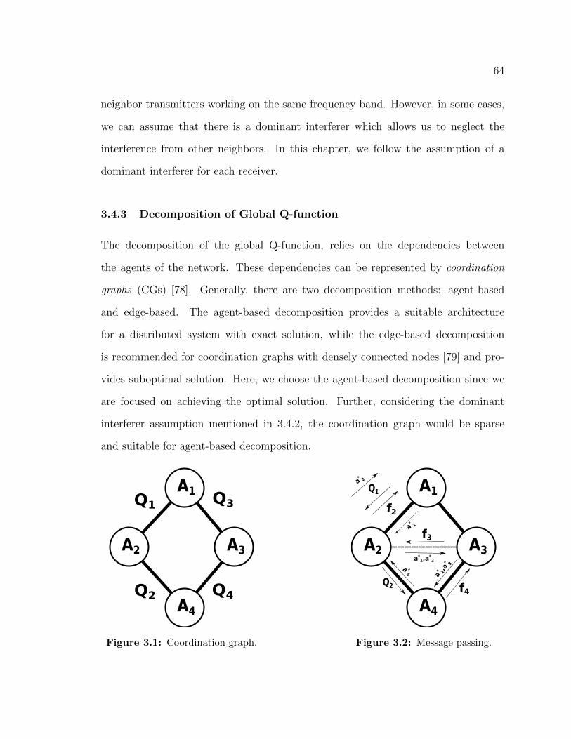
64
neighbor transmitters working on the same frequency band. However, in some cases,
we can assume that there is a dominant interferer which allows us to neglect the
interference from other neighbors. In this chapter, we follow the assumption of a
dominant interferer for each receiver.
3.4.3 Decomposition of Global Q-function
The decomposition of the global Q-function, relies on the dependencies between
the agents of the network. These dependencies can be represented by coordination
graphs (CGs) [78]. Generally, there are two decomposition methods: agent-based
and edge-based. The agent-based decomposition provides a suitable architecture
for a distributed system with exact solution, while the edge-based decomposition
is recommended for coordination graphs with densely connected nodes [79] and pro-
vides suboptimal solution. Here, we choose the agent-based decomposition since we
are focused on achieving the optimal solution. Further, considering the dominant
interferer assumption mentioned in 3.4.2, the coordination graph would be sparse
and suitable for agent-based decomposition.
A1
A2
A4
A3
Q1
Q4Q2
Q3
Figure 3.1: Coordination graph.
A1
A2
A4
A3
Q2
Q1
f2
f3
f4
a*1,a
*2
a* 1
a* 2,a
* 3
a* 2
a *4
Figure 3.2: Message passing.

65
In a wireless network, the Scope [Qj ] for agent j, is determined based on the
interference model of the system, which is related to set D in (3.1). In order to be
able to explain the proposed solution, we pick an example as in Fig. 3.1, in which four
agents interfere with each other. Assume that agent A1, receives interference from
A2 and A3, and A4 receives its interference from A2 and A3. Based on this model,
the coordination graph of the system is shown in Fig. 3.1. Each edge between agents,
shows a dependency between the two agents.
Here, we assume that all agents have the same state x, hence, Q (x, a) is written as
Q (a). According to the coordination graph in Fig. 3.1, the global Q-function, Q (a),
can be written as
Q(a) = Q1(a1, a2) +Q2(a2, a4) +Q3(a1, a3) +Q4(a3, a4). (3.9)
3.4.4 Coordinated Action Selection
In multi-agent Q-learning, according to (3.8), the agents select a joint action that
maximizes the global Q-function. By using the agent-based decomposition, the joint
action selection at state x, maxa Q (a), is written as
maxa1,a2,a3,a4
Q1(a1, a2) +Q2(a2, a4) +Q3(a1, a3) +Q4(a3, a4). (3.10)
This maximization problem, can be solved via variable elimination (VE) algorithm,
which is basically similar to variable elimination in a Bayesian network [80]. Here, we
review this method for the network in Fig. 3.1. The key idea is to maximize over one
variable at a time, find conditional solutions, passing conditional functions to other
agents, and sending back the results of local optimization to the related agents to

66
recover their joint action choices. The steps of the joint maximization solution are
presented in Fig. 3.2 as they are described below.
We start from agent A4. a4 influences Q2 and Q4, so the maximization problem
can be written as
maxa1,a2,a3
Q1(a1, a2) +Q3(a1, a3) + [maxa4
Q2(a2, a4) +Q4(a3, a4)]. (3.11)
Agent A2 communicates Q2 to A4, and A4 solves its local maximization, which results
in two functions: f4 (a2, a3), and b4 (a2, a3). These functions are defined as follows
f4 (a2, a3) = maxa4
Q2 (a2, a4) +Q4 (a3, a4) , (3.12)
b4 (a2, a3) = arg maxa4
Q2 (a2, a4) +Q4 (a3, a4) . (3.13)
At his stage, the A4 has a conditional solution for a4 based on a2, and a3, represented
as the function b4. Therefore, A4 keeps b4 and sends f4 to its connecting agent, A3.
Then, A4 is removed from the coordination graph, and the maximization problem is
translated to
maxa1,a2,a3
Q1 (a1, a2) +Q3 (a1, a3) + f4 (a2, a3) , (3.14)
f4 brings a new edge in the coordination graph, an induced edge, which is shown with
dashed line between A2 and A3 in Fig. 3.2. The next agent to be removed is A3. The
maximization problem is rewritten as

67
maxa1,a2
Q1 (a1, a2) +
[maxa3
Q3 (a1, a3) + f4 (a2, a3)
]. (3.15)
With the same procedure, A3 introduces f3 (a1, a2), and b3 (a1, a2). Accordingly, the
problem reduces to
maxa1,a2
Q1 (a1, a2) + f3 (a1, a2) . (3.16)
Next agent to choose its action is A2, for which the problem results in
f1 = maxa1
f2 (a1) , (3.17)
where, f2 (a1) = maxa2 Q1 (a1, a2) + f3 (a1, a2). Finally, A1 chooses its action based
on maximizing the function f2 (a1). The results at this stage are f1, and a∗1. f1
represents the maximum value of the global Q-function over a1, a2, a3, and a4, and a∗1
is the optimal joint action for A1. To recover the joint action choices, A1 sends a∗1 to
A2. Then A2 chooses its action, a2 = b2(a∗1), and sends a∗1, a∗2 to A3. A3 and A4 will
choose their actions with the same procedure, a∗3 = b3(a∗1, a∗2), and a∗4 = b4(a∗2, a
∗3).
In general, the elimination algorithm maintains a set of functions in each step,
Q. It starts with all local Q-functions, Q1, Q2, ..., QN, and eliminates agents one
by one. The algorithm steps can be summarized as follows
1. Choose an uneliminated agent, for example Al.
2. Choose all functions, Q1, Q2, ..., Ql ∈ Q whose Scope contains Al.
3. Define a new function, fl = maxal∑
j Qj and add it to Q. The Scope of Ql is
∪Lj=1 Scope [Qj]− Al.

68
3.4.5 Local Update Rule
After finding the joint action, each agent will update its local Q-function. The update
rule in (3.8) can be written as
∑j
Qj
(x, aj
)=∑j
Qj
(x, aj
)+
α
[∑j
Rj
(x, aj
)+ γmax
a
∑j
Qj (x′, a′)−∑j
Qj
(x, aj
)], (3.18)
where, the joint maximization is solved through VE according to the last section. By
assuming a∗ as the solution to the VE, and aj∗ ⊂ a∗ as the optimal joint action set
for Qj, the update rule for each local Q-function can be derived as
Qj(x, aj) = Qj(x, aj) + α[Rj(x, aj) + γQj(x′, aj
∗)−Qj(x, aj)]. (3.19)
The Fig. 3.2 illustrates all messages passed between the agents to solve VE and update
local Q-functions.
3.5 Power Allocation Using Coordinated Q-Learning
To integrate the idea of coordinated multi-agent learning into a communication net-
work, we will model the SBS as an agent, and the whole network as a multi-agent
MDP. The goal of the agents is to maximize total throughput of the network, as a
cooperative game. In the following we introduce the power allocation scheme based
on coordinated Q-learning as Q-CoPA.

69
3.5.1 Q-CoPA Algorithm
The proposed solution of this paper, Q-CoPA, can be summarized as follows
The interference model of the network will be used to derive the coordination graph
of the agents. The entire network is modeled as an MDP, and the global Q-function
of the MDP is approximated by linear combination of local Q-functions of the agents.
Each agent, based on the coordination graph, knows its Scope. Local Q-functions
are learned by the agents using cooperative Q-learning. The cooperation method
between the agents is to maximize the summation of local Q-functions by choosing
an appropriate joint action. This action selection is implemented using variable
elimination and message passing between the agents. The backhaul of the network
is used as the required infrastructure for message passing. The proposed method
is represented in Algorithm 1. In the Algorithm 1, the loops at lines 5 and 10 are
independent, and could be executed in parallel by the agents.
Algorithm 1 The proposed Q-CoPA algorithm
1: Initialize x2: Initialize All Qj(x, aj) arbitrarily3: for all episodes do4: Choose a∗ according to VE5: for all agents do6: Take action aj, observe Rj
7: end for8: Observe x′
9: Calculate maxa′ Q according to VE10: for all agents do11: Update local Q-function according to Eq. 3.1912: end for13: xj ← x
′j
14: end for

70
3.5.2 Q-learning Configurations
In the following the actions, and the reward of the Q-learning algorithm implemented
by each agent is defined.
• Actions : Each SBS has a set of actions, which is defined as the transmit power
levels. We define this set asp1, p2, ..., pNpower
. The number of power levels is
defined as Npower.
• Reward : In each episode, SBS chooses a power level, and transmits its data to
its intended user. The user measures the SINR of the signal, and will feedback it
to the SBS. Then the reward of the SBS j is calculated as rj = log2 (1 + SINRj).
3.6 Simulation Results
In this section, we implement the proposed power allocation for a two transmitter
and two receiver with interfering channels scenario. In fact, since there are only two
SBSs in the system, the assumption of one dominant interferer is accurate. Hence, we
can investigate the optimality of the proposed solution in this case. We consider each
SBS supports one UE. Each transmitter has omni-directional antenna and separate
power source. The channel model is assumed to be time-invariant, i.e. slow fading.
The channel gains are assumed to be g1 = 2.5, and g2 = 1.5. The P1,max = 10
dBm, P2,max = 13 dBm, and σ2 = 0 dBm. Without loss of generality we assume
that β1,2 = β2,1 = β in (3.1). The objective of the optimization is to find the power
allocation to maximize the sum throughput of the network under individual power
constraints.
In executing the Q-CoPA algorithm, each Q-function is defined as a table, Q-table.
The learning rate is α = 0.5, the discount factor as γ = 0.9, Npower = 100, and the

71
Figure 3.3: Global action-value function.
maximum number of episodes is set to 50 times the size of a Q-table. The MDP
of this problem is assumed to be stateless. The actions of agents are the transmit
powers, a1 = P1, and a2 = P2, Q-functions are defined as: Q1(P1,P2) and Q2(P1,P2),
and the global Q-function is defined as: Q (P1, P2) = Q1(P1, P2) +Q2(P1, P2).
According to [74], the optimal power allocation to maximize the sum-rate of the
above network is derived as
(P∗1,P∗2) =
(P1,max, 0), if g1P1,max ≥ max (g2P2,max, 1/β
2) ,
(0,P2,max), if g2P2,max ≥ max (g1P1,max, 1/β2) ,
(P1,max,P2,max), otherwise.
(3.20)
First we will execute our proposed algorithm for β = 0.3. According to the
optimal solution, (0,P2,max) is the optimal solution. According to Q-CoPA, the SBSs
will choose the powers that maximizes the global Q-function. The learned global

72
Q-function, Q (P1,P2), is plotted in Fig. 3.3 with maximum value at P1 = 0 and
P2 = P2,max, which is optimal.
0.0 0.2 0.4 0.6 0.8 1.0
Portion of Interference(β)
2
3
4
5
6
7
8
9
10
Norm
aliz
ed t
hro
ughput(bps/Hz) Q-CoPA
OptimumGreedySimultaneous
Figure 3.4: Normalized throughput versus portion of interference (β).
In Fig. 3.4, the solution of the power allocation for different values of the portion
of interference between two channels, β ∈ [0, 1], is plotted. The greedy approach is
defined to allocate full power to the transmitter with higher peak power, and zero
to the other one. The simultaneous allocation is defined to use maximum power at
both transmitters. According to Fig. 3.4, the Q-CoPA finds the optimal solution for
all values of β.
3.7 Conclusion
In this chapter, we used message-passing and variable elimination to coordinate the
power allocation in order to maximize a common goal in an interference-limited net-
work. The variable elimination algorithm is exact, so as long as the local Q-functions’

73
action set covers all interfering SBSs, the proposed solution is optimal. Although,
when each node of the coordination graph gets densely connected, i.e., the size of
action set of local Q-function grows, for the sake of computational complexity we
need to approximate local Q-functions’ action set with smaller sets, which results in
suboptimal solution. Therefore, the proposed solution is suitable for indoor applica-
tions, or networks in which the number of interferes is low.

74
Chapter 4
SPATIAL INDEXING FOR SYSTEM-LEVEL
EVALUATION OF 5G HETEROGENEOUS CELLULAR
NETWORKS
System level simulations of large 5G networks are essential to evaluate and design
algorithms related to network issues such as scheduling, mobility management, in-
terference management, and cell planning. In this chapter, we look back to the
idea of spatial indexing and its advantages, applications, and future potentials in
accelerating large 5G network simulations. We introduce a multi-level inheritance
based architecture which is used to index all elements of a heterogeneous network
(HetNet) on a single geometry tree. Then, we define spatial queries to accelerate
searches in distance, azimuth, and elevation. We demonstrate that spatial indexing
can accelerate location-based searches by 3 orders of magnitude. Further, the pro-
posed design is implemented as an open source platform freely available to all. This
work is submitted for possible publication in [29]
4.1 Introduction
Supporting the expected cellular traffic growth is one of the main tasks for the
next generation (a.k.a “5G”) wireless cellular networks and densification is one of
the main technologies to achieve such growth [3]. A key driver for densification in

75
the next 5-10 years will be small base stations (SBSs) operating at millimeter wave
(mmWave) frequencies. These SBSs will also support conventional communication
below 6 GHz (Sub6GHz) frequencies and possibly use mmWave for the backhauling
as well as some user equipment (UE) connections. Furthermore, due to propagation
features in mmWave bands, usage of highly directional antennas at the transceivers is
a necessity [16]. Hence, 5G will contain directional heterogeneous networks (HetNets)
with large number of nodes working on different frequency bands.
In the development and standardization of 5G, simulations are necessary to im-
plement and design new algorithms and protocols. Considering the above features of
5G, system-level simulations need platforms which deliver accurate results in short
time in large HetNets. These simulations are needed to evaluate the performance of
scheduling algorithms, mobility managements procedures, interference management
methods, and cell planning algorithms [81].
In simulation of large networks, operations that require searches over various nodes
of the network may be extremely time consuming, where spatial indexing has been
one of the methods to address this issue [82]. In fact, spatial indexing has been used
instead of traditional array indexing in order to accelerate location-based searches
in the simulation of large homogeneous networks such as wireless sensor networks
(WSNs). Wireless sensors are indexed based on their location on a geometry tree to
provide fast search queries. This method can not be trivially applied in HetNets since
a single geometry tree cannot be used for spatial indexing of different nodes.
4.1.1 Contributions
In this chapter, first, we propose a multi-level inheritance based structure to be able
to store different nodes of a HetNet on a single geometry tree. The proposed structure

76
is polymorphic in a sense that different levels of a node can be accessed via dynamic
casting [83]. Second, we focus on potentials of spatial indexing in accelerating the
simulation of directional communications. We introduce different spatial queries
and show that spatial indexing significantly accelerates simulation time in orders
of magnitude when it comes to location-based searches over azimuth, and elevation
as well as its traditional usage in searches over distance.
4.1.2 Motivation
Traditional wireless network simulators such as Network Simulator (NS-2, NS-3) [84,
85] do not take into consideration the relationship between a terminal and its location
in the indexing procedure. In other words, nodes are indexed based on features such
as identification numbers or the order in which they are added to the network. Nodes
are simply stored in an array (array indexing) and there is no pre-processing (sorting
or classification) based on the location of the nodes. Consequently, in a network
with n nodes, the search size of any algorithm related to the location of the nodes
equals the total number of the nodes in the network, i.e., O(n). Hence, if all nodes
run such an algorithm, the exhaustive search complexity would be O(n2). This is
important since in dynamic wireless networks, location-dependent searches are called
frequently in simulations. Examples of location-dependent searches in a simulation
environment are: finding the nearest neighboring users for association or handover
purposes, finding the k-nearest neighboring BSs for coordinated multipoint (CoMP)
transmission, or finding the potential interferers to evaluate signal-to-interference-
plus-noise-ratio (SINR) of a communication link. While the above searches are defined
over distance, in mmWave applications the direction of communication is important
as well. This means searching over distance, azimuth, and elevation at the same time

77
which can increase the complexity of the overall algorithm significantly. In practice,
decreasing the order of search complexity can potentially change the computation
time from hours to seconds of computation in large networks. In order to achieve this
goal, location-transparency can be changed into location-dependency in the indexing
of nodes [86–88]. To this aim, spatial indexing has been used in homogeneous networks
with the intent of accelerating distance queries. In this work, we take advantage of
polymorphic programming to use spatial indexing in heterogeneous cellular networks
and to provide fast spatial search queries in distance, azimuth, and elevation.
4.1.3 Related Works
There are several open-source simulators developed for different purposes in wireless
networks. In this category, with the focus on open-source platforms, we have Net-
work Simulators (NS-2, NS-3) [84, 85], OMNET++ [89], J-Sim [90], and SHOX [91]
platforms. These common simulators focus on preparing a platform for design and
evaluation of communication protocols in the network layer or layers above it. The
physical layer modules in the above platforms are not appropriate for mmWave
or directional communications. The full-stack mmWave module proposed by [92]
alleviates this shortcoming, by adding this module to the NS-3 platform for support
of the mmWave communications. The physical-layer module presented by [92] is
extensive. However, the added module is built on the core of the NS-3 and is not
designed to calculate directional interference in networks with dynamic topology.
Nevertheless, none of the above simulators takes advantage of spatial indexing. In
fact, the nodes of the network are simply stored in an array.
Spatial indexing has been used in two major applications in wireless commu-
nications: (i) location-aware data indexing in wireless broadcast systems and (ii)

78
location-dependent indexing in simulation platforms. Location awareness is naturally
the first step of context-awareness in broadcast systems and spatial indexing is used
in wireless broadcast systems where efficient indexing of data segments is essential for
mobile users to find their required query from the broadcast data [93–95]. Apart from
the application of spatial indexing in broadcast systems, its advantage in simulation
environments has been noticed in a few works [96,97]. Fast distance query of spatial
indexing is used in high fidelity large-scale simulation of wireless communications [96].
Also, [97] changed the indexing procedure of NS-3 in the simulation of a large-scale
(more than 1000 nodes) vehicular ad-hoc network (VANET) to provide fast distance
queries as well. However, wireless networks and more specifically cellular networks
are heterogeneous. This means elements of the network can vary from macro base
stations to small base stations and mobile users. Further, there are certain phenomena
that need to be considered in system-level simulations such as blockages. Also, in
5G, features of millimeter-wave communications such as directionality changes the
complexity of location-dependent searches. In fact, search queries are not just in
distance but also in azimuth and elevation as well. Therefore, we need an architecture
that uses spatial indexing in a HetNet and supports the above features. In the
following, we introduce a generic architecture that uses multi-level inheritance and
polymorphism to enable indexing a heterogeneous network on a single geometry
tree. Then we evaluate the performance of the proposed architecture with respect to
traditional array indexing.
It is worth mentioning that acceleration of high-fidelity wireless communication
simulations has been investigated through geography-based partitioning for parallel
implementation on multiple processors as well [98]. However, parallel computing is
not the focus of this work.

79
Figure 4.1: The proposed multi-level architecture. Location and geometry propertiesof elements of the network are abstracted in the Node object. The Container stores theelements of the network on a geometry tree. From the view of the geometry tree, allelements are the same and represented as polygons. The Network basically represents anywireless network which can be a WSN, mmWave, or an integrated access and backhaul(IAB) network.
4.2 Spatial Indexing and Queries in HetNets
In this section, we first introduce the architecture which enables us to use spatial
indexing for a HetNet. Then, the indexing procedure and the defined spatial queries
are explained.
4.2.1 Architecture
In order to store heterogeneous nodes on a single geometry tree, nodes of the network
need to be represented just by their geometry. In fact, the elements of the network
are abstracted as polygons regardless of their higher level nature which can be a UE,
BS, or even a blockage. The proposed architecture is shown in Fig. 4.1. All the
elements of the network are generated based on inheritance from an object named
Node. The Node object contains location and geometry (length, width, and height)
of the elements and is the lowest level in the platform and is stored on the geometry

80
tree. Node is inherited by the TRX and the Blockage objects. The TRX object
contains related parameters to a transceiver such as the carrier frequency, transmit
power, and antenna properties. Also, the TRX contains an independent standard
thread with signal-slot capabilities. The signal-slot methods are used to implement
message-passing and event-based processes such as asynchronous procedures of the
network. Wireless sensors, mmWave or Sub6GHz BSs, and UEs can be generated by
inheriting from the TRX. The blockage objects are generated by directly inheriting
from the Node. The proposed design consists of a class named Container which is used
to manage all the created nodes in the simulation. The Container holds a geometry
tree which indexes all the generated elements and provides the spatial queries over
the geometry tree. Since just the Node data is saved on the geometry tree, one single
tree can be used for any type of element in the network. The designed architecture
and indexing procedure is applicable to any object-oriented language that supports
multilevel inheritance. However, the code snippets that we use are based on C++
language.
4.2.2 Indexing a HetNet With single Geometry Tree
In order to use spatial indexing, a proper spatial data structure should be selected.
Most of the spatial data structures work based on the principle of space partitioning
and storing data on a tree-like structure such as R-tree or K-d tree [99]. K-d tree
can only contain points and does not handle adding and removing points. However,
in R-tree nodes are represented as polygons. Since, we need to provide dimensions
for the nodes of the network as well as dynamic removal of them, we use R-tree [100]
for spatial indexing. R-tree is a geometry tree proposed by Guttman as a dynamic
indexing structure designed for spatial searching in multi-dimensional datasets. Basi-

81
(a) (b)
Figure 4.2: Example of a HetNet indexed with a single R-tree with n = 10 and M = 3.(a) The tree containing different levels of MBRs which partition a network of one macroBS (MBS), four SBSs, four UEs, and one blockage. (b) The rectangles R1 to R17 representMBRs, the black MBRs (R1, R2) are the roots, the red MBRs (R3-R7) are the secondlayer, and the green MBRs (R8-R17) are the leaf nodes which contain the data objects ofthe network. The MBRs R1 and R2 cover total area of the network.
cally, R-tree groups the objects using minimum bounding rectangles (MBR). Objects
are added to an MBR within the index that will lead to the smallest increase in its
size. R-tree records the indices in its leaf nodes with pointers to the data objects
as in Fig. 4.2(a). Data objects refer to the polygons of the elements of the network
which is detailed below. Further, by defining M as the maximum number of entries
in an element of the tree, the average search complexity of R-tree is O(logM n). A
representation of the R-tree and MBRs over a HetNet is illustrated in Fig. 4.2(a) and
Fig. 4.2(b), respectively.
According to Fig. 4.2(a), the leaf nodes store data objects related to the elements
of the network. The data objects are 2-tuples containing first the location of the
element, and second a pointer to the Node object of the element. We name the
2-tuple, value pairs in the code snippets. We define the following value pair as the
input of the R-tree.

82
Node TRX
SBS
R14 R15
Node TRX
UE
<location,node*> <location,node*>
(a) (b)
Figure 4.3: (a) The value pairs of the R-tree leaves and their relationship with the elementsof the network. Each leaf contains location and a pointer which stores the Node informationof the respective element of the network. Here, R14 contains the location of a SBS and itsNode data. (b) Retrieving higher levels of an object from a query result.
1 typede f pair<point , shared ptr<node>>value ;
According to the above, an element of the network is added to the R-tree based on
its location (point variable) and a pointer (shared ptr) to its Node object and the
R-tree indexes the elements of the network based on their corresponding locations.
Fig. 4.3(a) shows the value pairs of MBRs R14 and R15 defined in Fig. 4.2(a). For
details of inserting elements to the R-tree see Appendix B.1.
4.2.3 Spatial Queries
A spatial query is a query which considers the spatial relationship between the
elements of the network such as relative location-based searching, k-nearest neighbors,
and ray tracing. Spatial queries have significant applications in map servers where
there are continuous queries over the database based on the location of the objects.
Google Maps and Quantum Geographic Information Systems (QGIS) are examples
of applications which use spatial queries frequently. Considering the above, any
location-dependent search can be defined as a spatial query over the polygons of
the elements of the network. For instance, finding fixed-radius neighbors can be

83
defined as a circle-shaped polygon query over the nodes of the network. Therefore,
we can represent the association of users to base stations as a spatial query. The same
applies to finding the potential interferers in a certain direction which can be stated
as a triangular-shaped polygon query. In the following, we describe these queries.
After inserting all the elements (BSs, UEs, blockages) in the R-tree, any element
is able to define customized spatial queries over the network. The general format of
a spatial query is defined as follows.
1 m tree . query ( Condition , Resu l t s )
In the above, the Condition can be any function defined based on the point variables.
Results is a standard vector containing the value pairs of the elements that their
locations satisfy the defined Condition. Due to the indexing method, any query over
the network results in a vector containing pointers to Node objects. In order to derive
the higher levels of a Node object, for example a mmWave BS from the pointer of its
Node, we use dynamic cast as in Fig. 4.3(b). It is important to note that since we
use downcasting to derive classes from the shared pointer of the Node, the Node class
should be polymorphic [83], i.e., Node should at least contain one virtual method.
Here, we use spatial queries to define two common location-dependent searches
in wireless networks: search for fixed-radius near neighbors and search for interferer
BSs residing in the boresight of a receiver. However, any customized query can be
defined as well. The two queries are implemented as follows.
(i) Fixed-radius near neighbors: This query is used in association, coordination,
and routing problems. The Condition for this query is written based on the euclidean
distance from the desired point. In fact, any point that is in distance R of the desired
point is in a circular polygon with radius R around the desired point. If the MBR
of any element of the network intersects with the defined circular polygon, then the

84
(a)
Receiver
Transmitter
InterfererNon-interferer
Trasmission Range
Beamwidth
Triangular polygon
(b)
Figure 4.4: (a) Sectored-pattern antenna model with the beamwidth of φm, main-lobe gainof Gmax, and side-lobe gain of Gmin. (b) Polygon estimating the area in which potentialinterferer BSs reside.
element is in distance R of the desired point (center of the circular polygon). In
the following the elements located in the defined distance R of the desired point are
derived.
1 // Def in ing the r e s u l t vec to r
2 std : : vector<value>r e s u l t s ;
3 // The d e s i r e d l o c a t i o n .
4 po int d e s i r e d ( xx , yy ) ;
5 m tree . query ( bgi : : s a t i s f i e s ( [ & ] ( va lue const& v ) re turn bg : : d i s t anc e ( v .
f i r s t , sought )<R; ) , s td : : b a c k i n s e r t e r ( r e s u l t s ) ) ;
(ii) Directional interferer neighbors: This query is used for SINR calculation
of a directional wireless link. In another terms, search for neighbors in distance
and azimuth (or elevation) at the same time. In directional communications, the
power received at the receiver depends on the combined antenna gain of the receiver
and transmitter. Directional communication is viable with large antenna arrays and
using different MIMO transmission techniques such as fully digital, analog or hybrid
beamforming. Here, we use the sectored-pattern antenna gain shown in Fig. 4.4(a)

85
which is practically accepted for single stream analog beamforming [16]. In order
to accurately calculate the antenna gain at a receiver, we need to figure out if the
interfering transmitter is in the main lobe of the receiver or not. We solve this
problem with a polygon query. In order to define this query, we define a triangular
polygon estimating the area in which the BSs causing interference are located as in
Fig. 4.4(b). The nodes residing inside the triangular polygon are in the main lobe of
the receiver. After finding the interferer nodes, we can initiate the same query from
the interfering nodes to see if the receiver is in their main lobe as well. This query
can be implemented as follows.
1 // Def in ing the r e s u l t vec to r .
2 std : : vector<value> r e s u l t s ;
3 // Performing the query to search f o r any node i n t e r s e c t i n g with the
der ived polygon .
4 m tree . query ( bgi : : i n t e r s e c t s ( t r i a n g u l a r p o l y g o n ) , std : : b a c k i n s e r t e r (
r e s u l t ) ) ;
In the above, the triangular polygon is defined for a transmitter-receiver pair based
on the direction of transmission, beamwidth, and the maximum transmission range
according to Fig. 4.4(b). The neighbors whose MBR intersect with the triangu-
lar polygon are returned in the results vector. By using dynamic cast the TRX related
object of the neighbors can be derived. Finally, the interference can be calculated
based on the interference model of the network. It is worth mentioning that the
polygon query can be used for other purposes such as user association for BSs which
have multiple sectors as well.

86
4.3 Simulation Acceleration with Spatial Indexing
The goal of this section is to compare the performance of spatial indexing versus array
indexing in location-dependent searches in large directional wireless networks. The
network under study contains mmWave SBSs which are distributed with fixed density
of 100 SBS/Km2. We assume SBSs are equipped with directional antennas. Without
loss of generality, we assume all SBSs are on the same horizon plane. Thus, we do
not consider beams variations in the elevation and define the antenna gain pattern
with widely-adopted sectorized-pattern as [16,101].
Generally, in cellular communication, the measured signal at a receiver is a combi-
nation of the desired signal, the interference, and noise, hence SINR. In mmWave com-
munications, due to narrow beams, the links are sometimes assumed to be interference-
free and the SNR metric is used in simulations. Despite the fact that the interference-
free assumption is reasonable, the probability of occurrence of interference increases as
the density of the network increases [59,102]. Selection of the right metric is important
in certain applications such as path selection and routing algorithms. Hence, we
assume two scenarios: (i) SNR and (ii) SINR calculation of all potential links between
any two pair of SBSs with maximum transmission range of 200 m.
In the following we provide performance time comparison and complexity analysis
in both scenarios. Experiments are carried out in C++ with an Intel(R) Core(TM)
i5-6300HQ @ 2.30 GHz processor powered by Fedora 31 operating system and Linux
kernel 5.4.18.

87
101
102
103
104
105
number of nodes
10-4
10-2
100
102
104
Pro
cessin
g tim
e (
s)
Spatial indexing search time
Array indexing search time
(a)
101
102
103
104
105
number of nodes
10-4
10-2
100
102
104
Loadin
g tim
e (
s)
Spatial indexing
Array indexing
(b)
Figure 4.5: (a) Processing times to calculate SNR of all existing links. (b) Loading timeto generate and store all nodes.
4.3.1 SNR calculation
In order to calculate the SNR of all potential links between SBSs in a network, we need
to measure distance of all pairs of SBSs and calculate SNR of the ones in transmission
range of each other. In array indexing, complexity of finding potential links between
one SBS and its neighbors is O(n), which contains measuring the distance between
the node and all existing nodes. Hence, the total complexity for all the nodes isO(n2).
However, with spatial indexing, finding neighbors can simply be implemented with a
fixed-radius neighbor query as in 4.2.3 which is a spatial query over the distance. The
complexity of one query is O(log n) and hence for the whole network is O(n log n)
on average. In Fig. 4.5(a) the processing time for finding the potential links for
calculating SNR of the network is presented. As shown, spatial indexing outperforms
array indexing.
It is worth mentioning that, when using spatial indexing, loading the nodes on
the R-tree introduces an overhead to the simulation. However, loading time is a
one-time overhead, however, location-dependent searches are called frequently during

88
101
102
103
104
105
number of nodes
10-4
10-2
100
102
104
Pro
cessin
g tim
e (
s)
Spatial indexing search time
Array indexing search time
Figure 4.6: Processing time to calculate SINR of all existing links.
a simulation. In Fig. 4.5(b), we have compared the required time of storing nodes on
an array and a R-tree with respect to the number of nodes.
4.3.2 SINR calculation
In directional communication, the calculation of SINR for a link contains one ad-
ditional search compared to SNR calculation. In fact, after finding the potential
neighbors, we need to search for interferers for each link. This search is in distance and
azimuth according to Fig. 4.4(b). With array indexing, finding directional interferers
for each link leads to another search which increases the complexity to O(n2). Hence,
the computational complexity for the whole network can go up toO(n3). On the other
hand, spatial indexing provides a systematic approach to accelerate the calculation of
SINR. SINR calculation can be simply implemented as a combination of fixed-radius
near neighbors query followed by a triangular polygon query over the results of the
first query. This systematic approach is one of the advantages of spatial indexing.
In Fig. 4.6, the processing time of SINR calculation in large wireless networks with
directional communication is plotted. As it is shown in Fig. 4.6, spatial indexing

89
has clear advantage in processing time of searches in distance and azimuth. This
advantage can be used to enormously accelerate system-simulation of large systems.
For the implementation details see Appendix B.3.
4.4 Conclusion
In this chapter, we propose the use of spatial indexing in system-level evaluation of
5G heterogeneous cellular networks. We introduced an inheritance based polymorphic
architecture which enables us to index a wireless heterogeneous network with a single
R-tree. This structure enables us to take advantage of spatial queries to accelerate
simulation of large-scale directional heterogeneous wireless networks. Researchers can
use spatial indexing in their platforms to accelerate system-level simulations enor-
mously. Acceleration can be achieved in any search defined in distance, azimuth or
even elevation. Further, due to the ability of considering the blockage, spatial indexing
can accelerate system-level simulations which account for the spatial correlation of
blocking such as [103, 104]. Another main application of spatial indexing could be
generating training data sets of accurate SINR values in millimeter-wave commu-
nications for machine learning purposes. Further, spatial indexing can accelerate
simulation in multiple applications such SINR evaluations in ad-hoc networks, node
deployment [105–107], routing, clustering, implementation of self-organizing networks
(SONs) [27], and generating communication graphs. We are currently developing an
open-source platform based on the introduced structure in Fig. 4.1 which implements
some of the applications of spatial indexing in [108].

90
Chapter 5
TOPOLOGY MANAGEMENT IN MILLIMETER WAVE
WIRELESS BACKHAUL IN 5G CELLULAR NETWORKS
The dynamic and autonomous connections of a mmWave backhaul network is similar
as an ad hoc network. In ad hoc networks, the topology of a network is the set
of communication links between the nodes that is used by the routing algorithm.
According to ad hoc related literature, weeding out redundant and unnecessary
topology information is called topology management. Topology management plays
a key role in performance of routing, scheduling, broadcasting. The wrong topology
information can reduce the capacity, increase the end-to-end delay, and decrease the
robustness to node failure. As the above factors are important in ad hoc networks,
they have the same importance in mmWave backhaul networks as well. In this
chapter, we investigate the effect of using signal-to-noise-ratio (SNR) instead of signal-
to-interference-plus-noise-ratio (SINR) in topology management of dense mmWave
networks. Further, we design a multi-agent reinforcement learning algorithm to
achieve k-connecitivty as one of the requirements of fail-safe wireless backhauling
in mmWave networks.

91
5.1 Introduction
Supporting the expected cellular traffic growth via densification is one of the main
tasks for the next generation (a.k.a “5G”) wireless cellular networks [3]. A key
driver for densification in the next 5-10 years will be small base stations (SBSs)
operating at millimeter wave (mmWave) frequencies. These SBSs will also support
conventional communication below 6 GHz (Sub6GHz) frequencies and possibly use
mmWave for the backhauling as well as some UE connections. Small cells construct an
underlay of low-power and short-range, indoor and outdoor microcells, femtocells or
picocells [109]. New small cells are deployed in public and private infrastructures with
the vision of aggressive densification to provide the high speculated rate requirements
of 5G networks. Meanwhile, achieving the full potential of densification to improve
the spectral efficiency of access links runs into the significant bottleneck of efficient
backhauling.
Wired and wireless technologies can be used as backhaul solutions. Wired tech-
nologies such as fiber or xDSL have the advantage of high throughput, high relia-
bility, and low latency. However, wired solutions have high expenses and situational
impracticality in providing backhaul to a large number of small cells [15]. On the
contrary, wireless technology is a potential solution to provide a cost-efficient and
scalable backhaul support when wired solution is impractical [16]. Wireless backhaul
technologies can operate at Sub6GHz or mmWave bands. Sub6GHz wireless backhaul
has the advantage of non-line-of-sight (NLoS) transmission with the disadvantage of
co-channel interference and variable delay. In constrast, thanks to huge spectrum,
high directional transmission, and low delay of line-of-sight (LoS) links, mmWave
communications can be modeled as pseudo-wired communications without inter-

92
ference [18]. Therefore, mmWave communications are suitable candidates for the
backhaul of dense small cells.
As mmWave communication is a potential technology for the backhaul of dense
small cell networks, its high path loss and susceptibility to blockage needs to be
considered in backhaul management (planning) procedures. High path loss results in
a limited range of effective communication which is resolved by multi-hop transmis-
sions [110]. Multi-hop transmission increases the reliability of the links while intro-
ducing more delay [111]. Severe vulnerability to blockage at mmWave transmission
decreases link availability [16]. Link blockage is solely dependent on the placement of
transceivers and the context of the environment. Surviving a blocked link can be done
via beam switching and finding new unblocked directions between the transceivers.
However, due to channel sparsity in mmWave communications, the number of strong
feasible beam directions between a transmitter and a receiver is mostly on the order
of two or three [112]. On the other hand, due to spatial correlation of beams, there is
good chance of blockage for all beams in case of severe blockage for one of them [113].
Hence, detouring the blockage by using another SBS as a relay is a viable option in
wireless backhauling [114].
Therefore, a SBS needs to be aware of all possible links that it can establish
to provide its backhaul in case of failure of one of them. Thus, we need an au-
tonomous backhauling algorithm to realize a wireless backhaul which is fast (low
latency), reliable (failure resilient), and scalable. We can simplify such definition
as a self-organizing wireless backhaul algorithm. In fact, due to unplanned and
high density deployment of small cells, self-organizing network (SON) procedures
and tools are becoming essential including backhaul managements. SON promises
self-configuration, self-optimization, and self-healing procedures for wireless backhaul.

93
Self-configuration establishes the backhaul links with the appropriate neighboring
cells and alignment of transceiver antennas. Self-optimization manages possible inter-
ference with neighboring radios. Self-healing features in avoiding possible link failures
and contains necessary procedures in case of link failures due to specific propagation
features of mmWave communications such as susceptibility to blockage.
The dynamic and autonomous connections of a mmWave backhaul network is
similar as ad hoc network. In ad hoc networks, the topology of a network is the set
of communication links between the nodes that is used by the routing algorithm.
According to ad hoc related literature, weeding out redundant and unnecessary
topology information is called topology management [115,116]. Topology management
plays a key role in performance of routing, scheduling, broadcasting. The wrong
topology information can reduce the capacity, increase the end-to-end delay, and
decrease the robustness to node failure. As the above factors are important in ad
hoc networks, they have the same importance in mmWave backhaul networks as
well. This is part of the reason, in recent literature, researchers model mmWave
backhaul networks with graph theory and use the same protocols and concepts in
ad hoc networks to manage the topology of the network [117]. However, specific
propagation characteristics of mmWave communications and 3GPP requirements for
mmWave backhaul in 5G NR [118] brings certain features that need to be considered
in topology management of mmWave networks. In this chapter, we aim to review
and analyze the requirements and possible topologies of mmWave networks.
5.1.1 Related Work
A great deal of research exists in different aspects of wireless backhauling. We can
roughly categorize recent works as in wireless backhaul technologies [18, 119], rate

94
and coverage analysis [120–123], optimal node deployment [124, 125], routing and
scheduling [126, 127], and management algorithms [117, 128–132]. In [18] hetero-
geneous backhaul operating on both Sub6GHz and mmWave bands is proposed as
a potential solution to backhauling of dense small cells due to their diverse char-
acteristics. Sub6GHz wireless backhaul has the advantage of NLoS transmission
with disadvantage of co-existence interference and unpredictable delay. MmWave
offers high capacity and reliability in LoS transmissions. The authors in [18] suggest
Sub6GHz band for modest length and mmWave as a competitive candidate for short
length communications. Meanwhile, the authors in [119] point to high licensing cost
of Sub6GHz wireless backhauling compared to the license-exempt nature of 60 GHz
from an operator’s perspective.
In [120] the advantage of short-hop wireless backhauling is analyzed in terms of
the number of antenna requirements for the SBSs and throughput scalability. Sing
et al. [121] derive rate distribution of a mmWave wireless backhaul network with
orthogonal sharing of resources between access and backhaul, and show that the
spectral efficiency of mmWave networks increases with density of SBSs. In [122]
and [123] integrated access backhaul (IAB) in mmWave communication is analyzed
in which access and backhaul share time and bandwidth resources, respectively.
More particularly, in [122] static and dynamic, synchronized and unsynchronized
time division duplexing (TDD) schemes and in [123] bandwidth sharing based on the
backhaul load are analyzed. In both scenarios, the higher achievable rate in dynamic
schemes are approved while [123] shows a cell-load beyond which the performance of
the IAB scheme starts decreasing.
Authors in [124] and [125] find optimal location of aggregator nodes (ANs), SBSs
with fiber-backhaul, to provide wireless backhaul to other SBSs of the network.

95
In [124] joint problem of minimizing deployment cost while maximizing coverage
via ANs is solved with Tabu search. In [125], wireless backhaul support for SBSs in
downtown Manhattan is considered. The authors find optimal location for deployment
of ANs that can establish LoS mmWave (60 GHz) links to gateways. The required
rate is delivered to the SBSs with deployment of two ANs that establish LoS mmWave
links to the SBSs in a noise-limited scenario, and six ANs that connect to SBSs via
NLoS Sub6GHz links in an interference-limited scenario. [126] and [127] consider
the problem of backhaul routing (path selection) in a wireless backhauled mmWave
network with already established links. The authors consider latency requirements of
the networks and find optimal routes via minimizing defined regret functions in [126]
and matching theory in [127].
In management of wireless backhaul, we need to make sure of a topology that is
configured cost-effectively, provides the required flow demand, and can restore itself
from link failures (self-healing) [128]. Generally, backhaul topology can be one of the
ring, tree or mesh topologies. The authors in [129] provide an analytical study of
the advantages of the mesh over tree and ring topologies in multiple aspects. They
characterize their problem with minimizing installation cost of wireless backhaul links
under traffic flow constraints and show that: (i) mesh topology can accommodate
higher traffic demands than tree and ring topology, (ii) mesh topology has higher
value for maximum feasible traffic fluctuations. Hence, mesh topology is of common
interest as the topology of wireless backhauls. As in terms of self-healing, in the
current cellular network and their predecessors, restorability is achieved with adding
backup links to the mesh of the network [130]. Authors in [117] and [131] follow the
same approach and design central organizing algorithms that add backup/redundant
links to achieve restorability and minimize packet loss in case of link failures. The

96
work in [131] considers a mmWave wireless backhaul network in which each SBS’s
antenna array is able to rotate mechanically. The work proposes a central software
defined solution to reconfigure the antennas’ alignment when the topology of the
network changes due to addition or reduction of SBSs or change of flow demand. The
work in [117] proposes a central solution to select some of the SBSs as cluster heads
to design a two-layer hierarchical mesh topology between the SBSs. Meanwhile, by
adding redundant paths for each non-cluster head SBS, they make sure of robustness
against blockage or link failures. The work in [132] focuses on the same idea of
selecting cluster heads, and provides a heuristic search algorithm to find a trade-off
between faster backhaul links or more cluster heads. However, their architecture does
not provide link failure restoration.
5.1.2 Contributions
The contributions of this chapter are two-folds.
1. We focus on the effect of selecting signal-to-noise-ratio (SNR) vs signal-to-
interference-plus-noise-ratio (SINR) as mmWave link quality performance in
dense mmWave networks. In fact, in directional communications, the links are
sometimes assumed to be interference-free, and the SNR metric is used in simu-
lations. Here, we show that despite the fact that in directional communications,
the interference-free assumption is reasonable, however, in cases of occurrence
of interference, SNR is not a valid metric and SINR should be considered to
make a correct decision.
2. We design a self-organizing algorithm to achieve k-connectivity in a backhaul
network. As we mentioned before, redundancy in a backhaul network is one of

97
the requirements of a fail-safe topology, and connectivity is a key performance
factor in topology management. Hence, we use reinforcement learning, Q-
learning in specific, to design a transmission range control algorithm to achieve
k-connectivity in a backhaul network.
The chapter is organized as follows. In Section 5.2, the system model is presented.
Section. 5.3 introduces distributed path selection policies and the effect of using SNR
instead of SINR on the resulted topology of the network. Section 5.4, introduced
the designed transmission range control algorithm. Finally, Section 5.5 concludes the
chapter.
Notation: Lowercase, boldface lowercase, boldface uppercase, and calligraphic
symbols represent scalars, vectors, matrices, and sets, respectively.
5.2 System Model
We consider a multi-cell heterogeneous network (HetNet) where multiple macrocells
are overlaid with a set of SBSs, S. SBSs are distributed with density λs = 100
SBSs/km2 on R2. The location of SBSs are derived according to a Poisson point
process (PPP) denoted by Φs, however, the derived conclusions in this chapter can be
considered for any network generation method. Fig. 5.1 shows the locations of MBSs
and SBSs. The network contains 66 wireless SBSs and 6 fixed wired BSs (MBSs). In
the following, the antenna, path loss, and interference models are detailed. Further,
the value of the system model parameters are presented in TABLE. 5.1.

98
-500 0 500
x-axis
-500
-400
-300
-200
-100
0
100
200
300
400
500
y-a
xis
SBS
MBS
Figure 5.1: Deployment models of mmWave base stations with density of 100 SBS/km2.MBSs are connected to the core network with a wired backhaul. SBSs use wirelessbackhauling to reach one of the MBSs. PPP distribution for SBSs and fixed locationsfor MBSs.
5.2.1 Antenna Model
We assume transmitters and receivers are equipped with directional antennas. With-
out loss of generality, we assume all BSs are on the same horizon plane. Thus, we do
not consider beams variations in the elevation angle θ and define the antenna gain
pattern with widely-adopted sectorized-pattern as [16,101]
G(φ) =
Gmax, if φ ≤ |φm|
Gmin, otherwise,
(5.1)
where, φ and φm denote azimuth angle and antenna main lobe beamwidth, re-
spectively. Gmax and Gmin denote the antenna gains at main lobe and side lobes,
respectively.

99
Table 5.1: Notation, Simulation Parameters
Notation Parameter Value
λs SBS density 100 km−2
B mmWave bandwidth 400 MHzPt mmWave transmit power 30 dBmf mmWave carrier frequency 28 GHzζ standard deviation of path loss LOS = 7.6, NLOS = 7.9α path loss exponent LOS=2.0, NLOS=3.5β path loss at 1 m 70 dBGmax
Gmin
φm
main lobe gainside lob gainbeam-width
18 dB−2 dB10
NF Noise Figure 10 dBσ2N noise power −174 dBm/Hz+10 log10 (B)+NF
— Area of the simulation 1km2
— Minimum distance between SBSs 10 m— Maximum mmWave transmission
range200 m
5.2.2 Path Loss
The received power at y ∈ R2 from a transmitter at x ∈ R2 with power p (x) is
given by p (x)ψ (x,y)L (x,y)−1, where ψ (x,y) is the overall beamforming gain.
L (x,y) = β + 10α log (‖x− y‖) +χ is the associated path loss, where χ ∼ N (0, ζ2).
The parameters β, α, and ζ2 represent the path loss at 1 meter distance, the path
loss exponent, and the variance of the shadowing, respectively. For mmWave com-
munications, motivated by the model of [121], we accommodate different path loss
parameters for LoS and NLoS links in mmWave band. We assume small-scale fading
as Nakagami fading with the shape factor parameter as 2 and 3 for LoS and NLoS
links, respectively.

100
5.2.3 Interference Model
The SINR of the link between the transmitter i and receiver j is calculated as follows
Due to directional communication, a few transmitters affect the desired receiver [133].
Considering this fact, the setting for interference is as follows. Assume, small BSs
(SBSs) communication over backhaul links. In each time-slot, there are NT SBSs
transmitting. Hence, there are NT −1 interfering transmitters and Ij number of them
are in the interference area of the desired receiver j (SBSj). Therefore, the received
SINR of a link from the SBS i (SBSi) to the SBSj can be expressed as
SINRij =HijGiGjL
−1 (dij)
N0/Pt +∑Ij
k=1HkjGkGjL−1 (dkj), (5.2)
where the received signal and the interference power are normalized by the transmis-
sion power Pt. Hij = |hij|2 is the small-scale fading power of the channel between
the SBSi and the SBSj. dij is the distance between the two SBSs and N0 is the
thermal noise power. The set Ij is the interfering nodes active at the same time-slot
as the transmitter-receiver i and j. The value of the Gk , k ∈ Ij, is set by a Bernoulli
random variable in such a way that by probability p = φm2π
, Gj = Gmax and otherwise,
Gj = Gmin. By considering the allocated bandwidth between the SBSi and the SBSj
as Bij, the instantaneous achievable rate for the link is rij = Bij log (1 + SINRij).
5.3 Distributed Path Selection
In reality, the measured signal at a receiver is a combination of the desired signal,
the interference, and noise, hence SINR. However, in directional communications, the
links are sometimes assumed to be interference-free, and the SNR metric is used in

101
Table 5.2: Path selection policies for wireless mmWave backhauling.
Policy Metric Selection RuleHigh SNR First SNR Select the link with the highest SNR.
Wired First position and SNRSelect a wired BS if possible
otherwise use High SNR first.
Position Aware position and SNR
Select a link with the highest SNR
among those links with parentBSs closer to a MBS.
High SINR First SINR Select the link with the highest SINR.
simulations. Here, we show that despite the fact that in directional communications,
the interference-free assumption is reasonable, however, in cases of occurrence of
interference, SNR is not a valid metric and SINR should be considered to make a
correct decision. In this regard, first, we implement four path selection policies for
wireless backhaul routing as in Table. 5.2. Second, we show the performance effect of
selecting SNR and SINR as decision metrics.
5.3.1 Path selection policies
We use four policies for path selection as in Table. 5.2. The High SNR First, the
Wired First, and the Position Aware policies are suggested in [134] and [135]. These
three policies are defined based on metrics of position and link SNR. To see the effect
of decision making based on SINR, we define one more policy named High SINR First
which uses the SINR as its metric. The selection rule under each policy is defined in
Table. 5.2.
5.3.2 Effect of selecting SNR vs SINR as mmWave link quality metric
In order to evaluate the performance of the defined path selection policies, two
performance metrics are discussed: (i) required number of hops for a SBS to reach an

102
MBS, and (ii) quality of bottleneck links. These two metrics are discussed below. The
location of SBSs and MBSs in Fig. 5.1 are loaded for all simulations. The simulations
are implemented using our proposed platform in Chapter 4.
Required number of hops to reach an MBS
For each policy, we evaluate the number of hops that SBSs take to reach a wired BS
(MBS). The plot in Fig. 5.2(a) shows the fraction of connected SBSs with respect to
the number of hops. Further, the final selected paths for all four policies are visualized
in Fig. 5.2 as well. According to Fig. 5.2(a), the two policies relying on just the quality
of the link (SNR, SINR) fail to connect all SBSs by increasing the number of hops.
In fact, in both cases there are SBSs which fail to reach any wired BS. We see this
also in Fig. 5.2(b) and Fig. 5.2(c). On the other hand, in the two policies which use
the position of wired BSs, SBSs reach to a wired BS with a maximum of five hops
for 90% of the times. The Position aware policy performs slightly better than the
Wired first policy in Fig. 5.2(a). Further, the wired first policy results in a star-shape
topology as in Fig. 5.2(d). Hence, awareness of the positions of wired BSs enhances
the chance of reaching to the wired BSs.
On the comparison of choosing SINR instead of SNR, we can look at the different
paths selected by SBSs in Fig. 5.2(b) and Fig. 5.2(c). As shown, choosing SINR
metric in the simulations results in different routes which are potentially closer to the
reality of the network.
Quality of the bottleneck links
The bottleneck link is defined as the weakest selected link from the selected paths in
the network [135], and its quality can be a performance measure for a path selection

103
0 5 10 15 20
Hop count
0
0.1
0.2
0.3
0.4
0.5
0.6
0.7
0.8
0.9
1
Fra
ctio
n o
f co
nn
ecte
d S
BS
s
High SNR first
High SINR first
Wired First
Position Aware
(a) Number of hops to reach an MBS.
0
00
0
0 0
2
-1
3
-1
-1
1
-1
-1
-1
-1
2
-1
2
1
3
-1
1
-1
-1
2
-1
-1
-1
-1
-1
-1
-1
-1
1
2
1
-1
3
1-1
1
1
-1
-1
-1
-1
2
-1
1
3
-1
2
-11
1
1
2
3
-1
-1
-1
1
-1
-1
-1
(b) High SNR First.
0
00
0
0 0
2
2
-1
3
-1
2
-1
-1
-1
-1
2
-1
4
1
5
2
1
-1
4
-1
3
-1
1
-1
3
-1
-1
-1
3
2
1
-1
4
12
1
-1
5
3
3
2
3
1
1
2
-1
3
-11
-1
1
1
3
-1
-1
-1
1
4
-1
-1
(c) High SINR First.
0
00
0
0 0
1
1
1
-1
2
1
3
1
1
1
1
1
1
1
3
1
1
1
1
1
1
1
1
1
-1
1
1
1
1
1
1
1
1
1-1
1
1
2
1
4
1
2
1
1
1
2
1
11
1
1
1
1
3
1
1
1
-1
2
1
(d) Wired First.
0
00
0
0 0
3
2
2
3
3
1
3
2
2
1
2
3
2
1
3
2
1
3
2
3
2
3
1
2
3
2
2
3
1
2
2
1
2
13
1
2
2
1
5
2
2
1
1
3
4
3
21
1
2
2
2
4
4
1
1
4
3
1
(e) Position Aware.
Figure 5.2: The selected paths by following each of the four policies. The red nodesrepresent the wired BS, black nodes represent the wireless SBSs. The number on each BSshows the number of hops it takes to reach to a wired BS. This number is zero for a wiredBS and −1 for the ones with no route to a wired BS.

104
5 10 15 20 25 30 35
SNR
0
0.1
0.2
0.3
0.4
0.5
0.6
0.7
0.8
0.9
1C
DF
High SNR first
High SINR first
Wired first
Position Aware
(a) CDF of SNR of the bottleneck link.
-30 -20 -10 0 10 20 30 40
SINR
0
0.1
0.2
0.3
0.4
0.5
0.6
0.7
0.8
0.9
1
CD
F
High SNR first
High SINR first
Wired first
Position Aware
(b) CDF of SINR of the bottleneck link.
Figure 5.3: Empirical CDF over 1000 number of iterations for a fixed topology and 6number of wired BSs.
policy. The CDF of the bottleneck link’s SNR and SINR under the defined policies are
plotted in Fig. 5.3(a) and Fig. 5.3(b), respectively. The relative trend of the High SNR
first, Wired first, and Position aware policies are the same in both figures. In fact,
position aware methods (Wired First an Position Aware) gain higher performance
compared to HQF1. However, the actual quality of the link, i.e., its SINR, is much
different than the SNR. Furthermore, the SINR of the bottleneck link under the
HQF2 policy has a different trend. This is the result of different decisions under the
SINR metric. Therefore, considering SINR as the metric becomes essential in dense
networks [59,102,136].
Computation wise, calculation of directional interference is much higher than an
interference-free scenario, and this is one of the advantages of the proposed platform
in Chapter 4 which provides a systematic approach to accelerate the calculation of
SINR in highly dense environments. It is important to mention that, it takes about
just 12 seconds to provide the 1000 iterations of the above simulations. Each iteration
involves neighborhood search and calculation of directional interference for each of
105
the BSs. This is important, since in similar work [134], the CDF of bottleneck link
quality is plotted in steps which implies low number of iterations for the simulations
due to high computational complexity.
5.4 K-Connectivity with Multi-Agent Reinforcement Learn-
ing
In this section, we focus on designing a self-organizing algorithm for SBSs to achieve
k-connectivity in a backhaul network. As we mentioned before, redundancy in a
backhaul network is one of the requirements of a fail-safe topology. Each SBS needs to
hold a certain number of connections to its neighbors to ensure successful transmission
of its backhaul data to the core network. We define the degree of a SBS as the
number of connections it can establish with its neighbors. In a network of size n,
if the degree of a node is on the order of log (n), the network is connected with
high probability [137]. Transmission range control is one of the methods of achieving
different connectivity degrees for a node. In fact, with increasing the transmission
range (with transmit power control), the node can increase number of its neighbors
and hence increase potential connections.
In this section, the range control is presented as a RL problem in which each SBS is
an agent which controls its transmission range to achieve a certain connectivity level.
Hence, achieving the desired degree with limited transmission power is essential. In
the following, we use reinforcement learning, Q-learning in specific, to achieve node
degree of k for all SBSs.

106
5.4.1 Q-learning for range control
In order to use Q-learning, the following definitions are used in our method.
• Agent: each node (SBS) is considered as an agent in the network. The goal of
each agent is to learn the minimum transmission range to achieve k as its node
degree.
• Environment: The whole network is the environment of the Q-learning. The
environment contains all the nodes as its agents. From each node’s view, the
combination of all other nodes constitutes the environment.
• State set: The state set of each node is defined as the set of degrees that it can
hold with its neighbors. Here, we assume a set, S = 0, 1, 2, ..., kmax, as the
state set for all the nodes. The goal state for each node is the state k ∈ S.
• Action set: Each node has a limited transmission range, Rmax. Each agent se-
lects its transmission range according to a set of actions,A = ∆r, 2∆r, ..., Rmax,
∆r = Rmax
|A| .
• Reward function: The design of the reward function depends on the goal of
each agent. Here, the goal of the agent is to reach the state k ∈ S, i.e., select
a minimum transmission range to reach to k neighbors. If a node selects an
action a and reaches the state s ∈ S, the defined reward function is as follows
r (s, a) = e−(s−k)2 . (5.3)
The agents act independently. This means each node considers any other node
in its transmission range as its potential neighbor. This is due to the definition of

107
topology management in which an algorithm is designed to find potential links for
communication. Meanwhile, scheduling the links is the responsibility of scheduler. In
the training process, each agent selects a communication range in its current state
based on ε-greedy policy, transmits a message to find the number of its neighbors in
the selected range, and updates the corresponding value of the state-action set in its
Q-function according to the temporal-difference method as follows
Q (s, a)← Q (s, a) + α
γmaxa′
Q (s′, a′) + r −Q (s, a)︸ ︷︷ ︸temporal-difference
, (5.4)
in which, s, a, s′ represent the current state, the selected action, and the new state,
respectively. Also, α and γ are the learning rate and the discount factor. Each agent
runs the Q-learning algorithm for L episodes to train its Q-function.
After the training, each agent runs Algorithm 1 to select its neighbors. In Al-
gorithm 1, the goal state, i.e., k, can be selected to configure different connectivity
levels for the network. The higher the k, the higher connectivity level is derived for
the network. However, the SBSs need to track more links and use more power to
increase their transmission range. Hence, the overhead and consumed energy of the
network increases as well.
5.4.2 Resulted topology
In order to visualize the resulted topology of the designed algorithm above, a network
is generated with the same approach as in Section 5.2 with loading a predefined
network. The simulation parameters are presented in Table. 5.3.
Implementation of a MARL algorithm on such a large network is not conventional.

108
Algorithm 1 Transmission Range Control
1: Initialize: a = Rmax, rounds = 02: Find the initial state s3: while rounds > 0 do4: a = arg maxa′ Q (s, a′)5: Broadcast a message with a6: Receive message from others and calculate number of neighbors7: Calculate the new state s′
8: if s′ == k then9: break
10: else11: Update Q-function12: end if13: rounds← rounds− 114: end while
Table 5.3: Simulation Parameters
Parameters Value
Density of nodes 100 km−2
Maximum communication range (Rmax) 200 mGoal state (k) 3
Learning rate (α) 0.2Discount factor (γ) 0.99
ε 0.2Rounds 10

109
12
9
10
8
11
6
9
7
7
7
9
4
5
5
10
3
5
7
7
12
8
14
7
7
7
10
8
9
6
6
10
6
10
4
1313
5
8
11
12
5
5
4
6
8
11
8
5
6
96
9
12
8
7
8
10
12
109
8
7
(a) Maximum transmission range.
3
2
3
1
6
3
5
3
3
3
3
2
3
3
3
3
3
3
5
5
2
3
5
3
3
3
3
5
3
1
3
3
2
2
33
3
3
3
3
3
3
3
3
5
3
3
3
3
53
5
0
3
3
5
5
5
32
3
3
(b) Transmission range control with Q-learning.
Figure 5.4: Topology of the network. The number on each node represents its degree.
We took advantage of our designed platform in Chapter 4 to integrate RL procedures
in each SBS node. Reinforcement learning procedures are implemented with the help
of the open-source template-based C++ RLLib [138]. The RLLib template-based
classes fit mathematics of RL with the implementations. Further, we illustrate how
to implement multi-agent RL training procedure in parallel (asynchronous training)
in Appendix C.1. The scalability of the asynchronous multi-agent RL algorithm is
investigated in Appendix C.1 as well.
The generated network is shown in Fig. 5.4(a). The degree of each node in
Fig. 5.4(a) is the result of using the maximum transmission range. This is the first
topology of the network before running the Algorithm 1. The topology of the network
after the training and running Algorithm 1 is presented in Fig. 5.4(b).

110
5.5 Conclusion
In this chapter, we focused on topology management in mmWave backhaul networks.
First, we defined distributed path selection policies and illustrated that the effect of
using SINR instead of SNR as a metric for mmWave link quality is a necessity in dense
networks. We investigated the importance of proper mmWave link quality metric with
visualization of the resulted network topologies and CDF of bottleneck links. Second,
we focused on k-connectivity of backhaul networks and designed a self-organizing
algorithm to achieve k-connectivity via multi-agent reinforcement learning. We used
our designed platform in Chapter 4 to implement the designed topology management
algorithms. Further, the resulted topologies are visualized as well.

111
Chapter 6
CONCLUSION
The presented dissertation is an effort to realize, develop, and investigate potential
solutions and tools for data-driven decision making in self-organizing networks (SONs)
more specifically in cellular networks. We develop an reinforcement learning based
framework and develop multiple learning algorithms for transmit power control in
heterogeneous networks (HetNets). Generally, training machine learning applications
needs large amount of data measurements and there is a need in the communication
community of standard data sets such as MNIST [139] in image processing field.
Hence, we developed an open-source platform for simulation of large 5G cellular
HetNets based on spatial indexing. The platform is able to produce large amount of
accurate signal signal-to-interference-plus-noise-ratio (SINR) values in short amount
of time. Finally, we take advantage of the developed platform and study topology
management of dense millimeter wave (mmWave) backhaul networks. In the following
the major contributions of the dissertation are detailed, and possible future directions
are presented.
6.1 Summary
• Chapter 2: In this chapter, we focus on realization of self-organizing networks
(SONs) with reinforcement learning (RL). We look into transmit power control
112
in a dense heterogeneous network (HetNet) and rely on local SINR measure-
ments to make decisions. We design a general framework for reinforcement
learning applications. The proposed framework models a multi-agent network
with a single Markov decision process (MDP) that contains the joint action of
the all the agents as its action set. Then, we make two main assumption to
factorize the global MDP into local ones: (i) total reward is linear combination
each agents reward, and (ii) the transition probability of each agent’s MDP
depends just on its action. With these two assumptions, we define local inde-
pendent and cooperative learning (IL, and CL) methods for decision making.
Further, we propose a systematic approach to define a reward function that
maximizes the summation of achievable transmission rate of the network while
satisfying minimum requirements for all agents. Finally, we derive a minimum
bound on the sample complexity of the proposed learning methods to achieve
ε-optimality. The numerical results of this chapter illustrate the performance
of different learning configurations and reward functions. This chapter plays a
key role in the dissertation as the reinforcement learning framework is used in
other chapters as well.
• Chapter 3: In this chapter, we focus on transmit power control in an interference-
limited network of small base stations (SBSs). First, we define a global Q-
function relating to the whole network. Then, in order to factorize the global
Q-function, we feed the interference model of the network to the factorization
process. In fact, we investigate the effect of accurate MDP factorization on the
optimality of the solution. To di this, we assume each SBS receives most of
its interference from one neighbor. Hence, its transition probability function

113
depends on its action and the neighbor. With this assumption, we factorize the
global Q-function and use the variable elimination (VE) method to find joint
actions in the network. The agents use message-passing for passing conditional
solutions to each other. In the simulation section, we illustrate the optimality
of the proposed solution for a 2 by 2 transmit-receiver case.
• Chapter 4: In this chapter, we design a new architecture for system-level
simulations of large 5G networks. We had two motivations for developing a new
simulation platform: (i) we needed to design topology management algorithms
for large directional networks, and ((ii)) we needed a fast simulator to be able
to run reinforcement learning algorithms. However, the existing simulators did
not provide us with one. Hence, we looked back to the idea of spatial indexing
and its advantages, applications, and future potentials in accelerating large 5G
network simulations. We introduce a multi-level inheritance based architecture
which is used to index all elements of a HetNet on a single geometry tree.
Then, we define spatial queries to accelerate searches in distance, azimuth,
and elevation. The platform can be used to evaluate and design algorithms
related to network issues such as scheduling, mobility management, interference
management, and cell planning. Further, the proposed design is implemented
as an open source platform freely available to all.
• Chapter 5: In this chapter, we focus on topology management of mmWave
backhaul networks. First, we investigate the effect of using signal-to-noise-ratio
(SNR) instead of SINR in topology management of dense mmWave networks.
In mmWave communications, due to narrow beams, the links are sometimes
assumed to be interference-free and the SNR metric is used in simulations. De-
114
spite the fact that the interference-free assumption is reasonable, the probability
of occurrence of interference increases as the density of the network increases.
We investigate the effect of using SNR and SINR on final derived topology
of a mmWave backhaul network. Further, we design a multi-agent reinforce-
ment learning algorithm to achieve k-connecitivty as one of the requirements of
fail-safe wireless backhauling in mmWave networks.
6.2 Future Research Direction
6.2.1 Deep reinforcement learning for large state sets
As we discussed in simulation section of Chapter 2, there is a performance gap between
the proposed approach and the exhaustive search. In fact, we wish to improve and
cover this gap by utilizing deep neural networks (DNNs) as the function approximator
of the learning method. Neural networks can handle the large state-action spaces more
efficiently. Hence, by increasing the state set size we would like to decrease the gap
between the RL and the exhaustive search solutions.
6.2.2 Mean-field reinforcement learning in large networks
One of our future works is to extend the proposed message-passing based solution in
Chapter 3 to multi transmit-receiver pairs such as [140]. However, the overhead
of message passing between the agents would be enormous. Further more, the
assumption of one major interferer for each agent might not hold all the times in
cellular networks. We propose to use mean-field reinforcement learning [141], to
factorize the global Q-function. In fact the transition probability of each agent
would depend on its own action and an action which is the average of other agents
115
in the environment. Therefore, we might be able to apply the idea of VE and
message-passing in large networks as well.
6.2.3 Spatial correlation of blocking in HetNets
One of the features of the proposed platform in Chapter 4, is ability to introduce
blocking in the simulation environment. We believe spatial indexing can accelerate
system-level simulations which account for the spatial correlation of blocking as well.
Developing an application based on the core of the platform for such studies can be
a potential direction for extending the platform.
6.2.4 Graph embedding in topology management
We are currently working on the applications of graph embedding methods in topology
management of wireless networks. Topology management can be seen as an algorithm
which searches over possible graphs of the network to find one that satisfies all the
requirements. Designing an algorithm for search over a graph can be challenging.
We wish to overcome this difficulty by using graph embedding methods. In fact, we
would like to embed the graph of the wireless network into a fixed-dimensional vector
space. This approach helps to search in a vector space in efficient time. Further,
the designed machine learning algorithms can become independent of the size of the
graphs as well.

116
Bibliography
[1] SNS.Telecom&IT, “SON (self-organizing networks) in the 5G Era: 2019-2030-opportunities, challenges, strategies forecasts,” Tech. Rep., Sep 2018.
[2] R. S. Sutton and A. G. Barto, Introduction to Reinforcement Learning, 1st ed.Cambridge, MA, USA: MIT Press, 1998.
[3] J. G. Andrews, S. Buzzi, W. Choi, S. V. Hanly, A. Lozano, A. C. K. Soong,and J. C. Zhang, “What will 5G be?” IEEE J. Select. Areas Commun., vol. 32,no. 6, pp. 1065–1082, Jun. 2014.
[4] R. W. Heath, N. Gonzalez-Prelcic, S. Rangan, W. Roh, and A. M. Sayeed, “Anoverview of signal processing techniques for millimeter wave MIMO systems,”vol. 10, no. 3, pp. 436–453, Apr. 2016.
[5] L. Jiang and H. Jafarkhani, “Multi-user analog beamforming in millimeterwave MIMO systems based on path angle information,” IEEE Trans. WirelessCommun., vol. 18, no. 1, pp. 608–619, Jan. 2019.
[6] O. El Ayach, S. Rajagopal, S. Abu-Surra, Z. Pi, and R. W. Heath, “Spatiallysparse precoding in millimeter wave MIMO systems,” IEEE Trans. WirelessCommun., vol. 13, no. 3, pp. 1499–1513, Mar. 2014.
[7] J. Brady, N. Behdad, and A. M. Sayeed, “Beamspace MIMO for millimeter-wavecommunications: System architecture, modeling, analysis, and measurements,”IEEE Trans. Antennas Propagat., vol. 61, no. 7, pp. 3814–3827, July 2013.
[8] B. He and H. Jafarkhani, “Low-complexity reconfigurable MIMO for millimeterwave communications,” IEEE Trans. Commun., vol. 66, no. 11, pp. 5278–5291,Nov. 2018.
[9] M. A. Almasi, R. Amiri, H. Jafarkhani, and H. Mehrpouyan, “Mmwave lens-based MIMO system for suppressing small-scale fading and shadowing,” IEEETrans. Wireless Commun., 2020.
[10] M. A. Almasi, R. Amiri, and H. Mehrpouyan, “A new millimeter wave MIMOsystem for 5G networks,” arXiv preprint arXiv:1807.04851, 2018.

117
[11] M. A. Almasi, R. Amiri, M. Vaezi, and H. Mehrpouyan, “Lens-based millimeterwave reconfigurable antenna NOMA,” in Proc. IEEE ICC Workshops, pp. 1–5,May 2019.
[12] S. Shad, S. Kausar, and H. Mehrpouyan, “Waveguide-fed lens based beam-steering antenna for 5G wireless communications,” in Proc. IEEE Intern. Symp.on Antennas and Propagation, pp. 1149–1150, Jul 2019.
[13] S. Kausar, S. Shad, A. Kausar, and H. Mehrpouyan, “Design of high gainlow cost beam-steering reflectarray antenna,” in Proc. IEEE Intern. Symp. onAntennas and Propagation, pp. 315–316, Jul 2019.
[14] ——, “Design of high gain single layer reflectarray antenna using ring anddouble square elements,” in Proc. IEEE Intern. Symp. on Antennas and Prop-agation, pp. 293–294, Jul 2019.
[15] Y. Li, E. Pateromichelakis, N. Vucic, J. Luo, W. Xu, and G. Caire, “Radioresource management considerations for 5G millimeter wave backhaul andaccess networks,” IEEE Commun. Mag., vol. 55, no. 6, pp. 86–92, Jun. 2017.
[16] J. G. Andrews, T. Bai, M. N. Kulkarni, A. Alkhateeb, A. K. Gupta, andR. W. Heath, “Modeling and analyzing millimeter wave cellular systems,” IEEETrans. Commun., vol. 65, no. 1, pp. 403–430, Jan 2017.
[17] M. Gupta, A. Rao, E. Visotsky, M. Cudak, A. Ghosh, and J. G. Andrews,“Learning-based delay optimization for self-backhauled millimeter wave cellularnetworks,” in Proc. Asilomar Conf. on Signals, Systems and Computers, pp.1–5, Nov. 2019.
[18] G. Zhang, T. Q. S. Quek, M. Kountouris, A. Huang, and H. Shan, “Fundamen-tals of heterogeneous backhaul design–analysis and optimization,” IEEE Trans.Commun., vol. 64, no. 2, pp. 876–889, Feb 2016.
[19] S. Haykin, “Cognitive radio: brain-empowered wireless communications,” IEEEJ. Select. Areas Commun., vol. 23, no. 2, pp. 201–220, Feb 2005.
[20] E. Yanmaz, O. K. Tonguz, and S. Dixit, “Self-organization in cellular wirelessnetworks via fixed relay nodes,” in Proc. IEEE Globecom, pp. 1–5, Nov 2006.
[21] W. Elmenreich and H. de Meer, “Self-organizing networked systems for technicalapplications: A discussion on open issues,” Self-Organizing Systems, SpringerBerlin Heidelberg, pp. 1–9, 2008.

118
[22] 3GPP, “Study on the Self-Organizing Networks for 5G networks,” 3rd Gen-eration Partnership Project (3GPP), Technical Specification (TS) 28.861, Dec2019, version 16.0.0.
[23] O. G. Aliu, “Resource allocation in self organising cellular networks,” Ph.D.dissertation, University of Surrey, UK, 2012.
[24] J. Schulman, “Optimizing expectations: From deep reinforcement learningto stochastic computation graphs,” Ph.D. dissertation, EECS Department,University of California, Berkeley, Dec 2016. [Online]. Available: http://www2.eecs.berkeley.edu/Pubs/TechRpts/2016/EECS-2016-217.html
[25] C. J. C. H. Watkins and P. Dayan, “Q-learning,” Machine Learning, vol. 8,no. 3, pp. 279–292, May 1992.
[26] R. Amiri, H. Mehrpouyan, L. Fridman, R. K. Mallik, A. Nallanathan, andD. Matolak, “A machine learning approach for power allocation in HetNetsconsidering QoS,” in Proc. IEEE ICC, pp. 1–7, May 2018.
[27] R. Amiri, M. A. Almasi, J. G. Andrews, and H. Mehrpouyan, “Reinforcementlearning for self organization and power control of two-tier heterogeneous net-works,” IEEE Trans. Wireless Commun., vol. 18, no. 8, pp. 3933–3947, Aug.2019.
[28] R. Amiri, H. Mehrpouyan, D. Matolak, and M. Elkashlan, “Joint power alloca-tion in interference-limited networks via distributed coordinated learning,” inProc. IEEE Veh. Technol. Conf., pp. 1–5, Aug 2018.
[29] R. Amiri, E. Balevi, J. G. Andrews, and H. Mehrpouyan, “Spatial Indexingfor System-Level Evaluation of 5G Heterogeneous Cellular Networks,” to bepublished.
[30] O. G. Aliu, A. Imran, M. A. Imran, and B. Evans, “A survey of self organisationin future cellular networks,” IEEE Commun. Surv. Tutor., vol. 15, no. 1, pp.336–361, First Quarter 2013.
[31] J. Moysen and L. Giupponi, “From 4G to 5G: Self-organized networkmanagement meets machine learning,” CoRR, vol. abs/1707.09300, 2017.[Online]. Available: http://arxiv.org/abs/1707.09300
[32] J. G. Andrews, S. Buzzi, W. Choi, S. V. Hanly, A. Lozano, A. C. K. Soong,and J. C. Zhang, “What will 5G be?” IEEE J. Select. Areas Commun., vol. 32,no. 6, pp. 1065–1082, Jun 2014.

119
[33] M. Peng, D. Liang, Y. Wei, J. Li, and H. Chen, “Self-configuration and self-optimization in LTE-advanced heterogeneous networks,” IEEE Commun. Mag.,vol. 51, no. 5, pp. 36–45, May 2013.
[34] M. Agiwal, A. Roy, and N. Saxena, “Next generation 5G wireless networks:A comprehensive survey,” IEEE Commun. Surv. Tutor., vol. 18, no. 3, pp.1617–1655, Thirdquarter 2016.
[35] P. V. Klaine, M. A. Imran, O. Onireti, and R. D. Souza, “A survey ofmachine learning techniques applied to self-organizing cellular networks,” IEEECommun. Surv. Tutor., vol. 19, no. 4, pp. 2392–2431, Fourthquarter 2017.
[36] A. Imran, A. Zoha, and A. Abu-Dayya, “Challenges in 5G: how to empowerSON with big data for enabling 5G,” IEEE Network, vol. 28, no. 6, pp. 27–33,Nov 2014.
[37] R. Li, Z. Zhao, X. Zhou, G. Ding, Y. Chen, Z. Wang, and H. Zhang, “Intelligent5G: When cellular networks meet artificial intelligence,” IEEE Wirel. Commun.,vol. 24, no. 5, pp. 175–183, Oct 2017.
[38] V. Chandrasekhar, J. G. Andrews, T. Muharemovic, Z. Shen, and A. Gatherer,“Power control in two-tier femtocell networks,” IEEE Trans. Wireless Com-mun., vol. 8, no. 8, pp. 4316–4328, Aug 2009.
[39] Z. Lu, T. Bansal, and P. Sinha, “Achieving user-level fairness in open-accessfemtocell-based architecture,” IEEE Trans. Mobile Comput., vol. 12, no. 10,pp. 1943–1954, Oct 2013.
[40] H. Claussen, “Performance of macro- and co-channel femtocells in a hierarchicalcell structure,” IEEE 18th Int. Symp. Pers. Indoor Mobile Radio Commun., pp.1–5, Sep 2007.
[41] R. Amiri and H. Mehrpouyan, “Self-organizing mm-wave networks: A powerallocation scheme based on machine learning,” in Proc. IEEE GSMM, pp. 1–4,May 2018.
[42] Y. S. Nasir and D. Guo, “Multi-agent deep reinforcement learning for dynamicpower allocation in wireless networks,” IEEE J. Select. Areas Commun., vol. 37,no. 10, pp. 2239–2250, Oct. 2019.
[43] D. Lopez-Perez, X. Chu, A. V. Vasilakos, and H. Claussen, “Power minimiza-tion based resource allocation for interference mitigation in OFDMA femtocellnetworks,” IEEE J. Select. Areas Commun., vol. 32, no. 2, pp. 333–344, Feb2014.

120
[44] M. Yousefvand, T. Han, N. Ansari, and A. Khreishah, “Distributed energy-spectrum trading in green cognitive radio cellular networks,” IEEE Trans.Green Commun., vol. 1, no. 3, pp. 253–263, Sep 2017.
[45] H. Yazdani and A. Vosoughi, “On cognitive radio systems with directionalantennas and imperfect spectrum sensing,” in Proc. IEEE ICASSP, pp. 3589–3593, Mar 2017.
[46] A. Galindo-Serrano and L. Giupponi, “Distributed Q-learning for aggregatedinterference control in cognitive radio networks,” IEEE Trans. Veh. Technol.,vol. 59, no. 4, pp. 1823–1834, May 2010.
[47] H. Saad, A. Mohamed, and T. ElBatt, “Distributed cooperative Q-learning forpower allocation in cognitive femtocell networks,” in Proc. IEEE Veh. Technol.Conf., pp. 1–5, Sep 2012.
[48] J. R. Tefft and N. J. Kirsch, “A proximity-based Q-learning reward functionfor femtocell networks,” in Proc. IEEE Veh. Technol. Conf., pp. 1–5, Sep 2013.
[49] M. Bennis, S. M. Perlaza, P. Blasco, Z. Han, and H. V. Poor, “Self-organizationin small cell networks: A reinforcement learning approach,” IEEE Trans.Wireless Commun., vol. 12, no. 7, pp. 3202–3212, Jul 2013.
[50] B. Wen, Z. Gao, L. Huang, Y. Tang, and H. Cai, “A Q-learning-based downlinkresource scheduling method for capacity optimization in LTE femtocells,” inProc. IEEE. Int. Comp. Sci. and Edu., pp. 625–628, Aug 2014.
[51] Z. Gao, B. Wen, L. Huang, C. Chen, and Z. Su, “Q-learning-based power controlfor LTE enterprise femtocell networks,” IEEE Syst. J., vol. 11, no. 4, pp. 2699–2707, Dec 2017.
[52] M. Miozzo, L. Giupponi, M. Rossi, and P. Dini, “Distributed Q-learning forenergy harvesting heterogeneous networks,” in Proc. IEEE. ICCW, pp. 2006–2011, Jun 2015.
[53] R. Barazideh, O. Semiari, S. Niknam, and B. Natarajan, “ReinforcementLearning for Mitigating Intermittent Interference in Terahertz CommunicationNetworks,” arXiv e-prints, 2020.
[54] B. Hamdaoui, P. Venkatraman, and M. Guizani, “Opportunistic exploitation ofbandwidth resources through reinforcement learning,” in Proc. IEEE GLOBE-COM, pp. 1–6, Nov 2009.

121
[55] G. Alnwaimi, S. Vahid, and K. Moessner, “Dynamic heterogeneous learninggames for opportunistic access in LTE-based macro/femtocell deployments,”IEEE Trans. Wireless Commun., vol. 14, no. 4, pp. 2294–2308, Apr 2015.
[56] K.-L. A. Yau, P. Komisarczuk, and P. D. Teal, “Reinforcement learning forcontext awareness and intelligence in wireless networks: Review, new featuresand open issues,” J. Netw. Comput. Appli., vol. 35, no. 1, pp. 253 – 267, Jan2012.
[57] L. Matignon, G. J. Laurent, and N. Le Fort-Piat, “Reward function and initialvalues: Better choices for accelerated goal-directed reinforcement learning,” inProc. ICANN, pp. 840–849, 2006.
[58] Z.-Q. Luo and W. Yu, “An introduction to convex optimization for communi-cations and signal processing,” IEEE J. Select. Areas Commun., vol. 24, no. 8,pp. 1426–1438, Aug 2006.
[59] S. Niknam and B. Natarajan, “On the regimes in millimeter wave networks:Noise-limited or interference-limited?” in Proc. IEEE ICCW, pp. 1–6, May2018.
[60] H. Sun, X. Chen, Q. Shi, M. Hong, X. Fu, and N. D. Sidiropoulos, “Learning tooptimize: Training deep neural networks for interference management,” IEEETrans. Signal Processing, vol. 66, no. 20, pp. 5438–5453, Oct 2018.
[61] C. Boutilier, T. L. Dean, and S. Hanks, “Decision-theoretic planning: Structuralassumptions and computational leverage,” J. Art. Intel. Research, vol. 11, pp.1–94, Jul 1999.
[62] Z. Lin and M. van der Schaar, “Autonomic and distributed joint routing andpower control for delay-sensitive applications in multi-hop wireless networks,”vol. 10, no. 1, pp. 102–113, Jan 2011.
[63] C. Guestrin, M. G. Lagoudakis, and R. Parr, “Coordinated reinforcementlearning,” in Proc. ICML, pp. 227–234, Jul 2002.
[64] E. Even-Dar and Y. Mansour, “Learning rates for Q-learning,” J. Mach. Learn.Research, vol. 5, pp. 1–25, Dec 2004.
[65] L. Busoniu, R. B. ska, and B. D. Schutter, “A comprehensive survey of mul-tiagent reinforcement learning,” IEEE Trans. Syst., Man, Cybern. C, vol. 38,no. 2, pp. 156–172, Mar 2008.
[66] M. J. Kearns and S. P. Singh, “Finite-sample convergence rates for Q-learningand indirect algorithms,” NIPS, vol. 11, pp. 996–1002, 1999.

122
[67] 3GPP, “Evolved Universal Terrestrial Radio Access (E-UTRA); Further ad-vancements for E-UTRA physical layer aspects,” 3rd Generation PartnershipProject (3GPP), Technical Specification (TS) 36.814, 03 2010, version 9.0.0.
[68] C. C. Zarakovitis, Q. Ni, D. E. Skordoulis, and M. G. Hadjinicolaou, “Power-efficient cross-layer design for OFDMA systems with heterogeneous QoS, im-perfect CSI, and outage considerations,” IEEE Trans. Veh. Technol., vol. 61,no. 2, pp. 781–798, Feb 2012.
[69] X. Ge, S. Tu, G. Mao, C. X. Wang, and T. Han, “5G ultra-dense cellularnetworks,” IEEE Wireless Commun. Mag., vol. 23, no. 1, pp. 72–79, February2016.
[70] M. Chen, Y. Hua, X. Gu, S. Nie, and Z. Fan, “A self-organizing resourceallocation strategy based on Q-learning approach in ultra-dense networks,” inIEEE Int. Conf. on Network Infrastructure and Digital Content (IC-NIDC),Sept 2016, pp. 155–160.
[71] S. Lin, J. Yu, W. Ni, and R. Liu, “Radio resource management for ultra-densesmallcell networks: A hybrid spectrum reuse approach,” in Proc. IEEE Veh.Technol. Conf., June 2017, pp. 1–7.
[72] A. Galindo-Serrano and L. Giupponi, “Self-organized femtocells: A fuzzyQ-learning approach,” Wirel. Netw., vol. 20, no. 3, pp. 441–455, Apr. 2014.[Online]. Available: http://dx.doi.org/10.1007/s11276-013-0609-6
[73] T. Park, J. Jang, O.-S. Shin, and K. B. Lee, “Transmit power allocation for adownlink two-user interference channel,” IEEE Commun. Lett., vol. 9, no. 1,pp. 13–15, Jan 2005.
[74] D. Park, “Optimal power allocation in two-user interference channel underindividual power constraint,” in ICTC, Oct 2016, pp. 530–532.
[75] M. Chiang, C. W. Tan, D. P. Palomar, D. O’neill, and D. Julian, “Power controlby geometric programming,” IEEE Trans. Wireless Commun., vol. 6, no. 7, pp.2640–2651, July 2007.
[76] M. J. Osborne and A. Rubinstein, A course in game theory. Cambridge, USA:The MIT Press, 1994, electronic edition.
[77] J. R. Kok, M. T. Spaan, and N. Vlassis, “Non-communicative multi-robotcoordination in dynamic environments,” Robotics and Autonomous Systems,vol. 50, no. 2, pp. 99 – 114, 2005.

123
[78] C. Guestrin, M. G. Lagoudakis, and R. Parr, “Coordinated reinforcementlearning,” in Proc., ser. ICML, 2002, pp. 227–234.
[79] J. R. Kok and N. Vlassis, “Sparse cooperative Q-learning,” in Proc., ser. ICML.ACM, 2004, pp. 61–.
[80] C. Guestrin, D. Koller, and R. Parr, “Multiagent planning with factoredMDPs,” in Advances in Neural Information Processing Systems 14. MIT Press,2002, pp. 1523–1530.
[81] J. C. Ikuno, M. Wrulich, and M. Rupp, “System level simulation of LTEnetworks,” in Proc. IEEE VTC, pp. 1–5, May 2010.
[82] F. P. Preparata and M. I. Shamos, Computational Geometry: An Introduction.Berlin, Heidelberg: Springer-Verlag, 1985.
[83] B. Stroustrup, The C++ Programming Language, 4th ed. Addison-WesleyProfessional, 2013.
[84] T. Issariyakul and E. Hossain, Introduction to Network Simulator 2 (NS2),Springer, pp. 21–40, Boston, MA, 2012.
[85] G. F. Riley and T. R. Henderson, “The NS-3 network simulator,” Modeling andTools for Network Simulation, pp. 15–34, 2010.
[86] M. H. Dunham and V. Kumar, “Location dependent data and its managementin mobile databases,” in Proc. IEEE Workshop on Database and Expert SystemsApplications (DEXA), pp. 414–419, Aug. 1998.
[87] N. Marsit, A. Hameurlain, Z. Mammeri, and F. Morvan, “Query processing inmobile environments: a survey and open problems,” in Proc. IEEE Int. Conf.on Distributed Frameworks for Multimedia Applications, pp. 150–157, Feb. 2005.
[88] A. Y. Seydim, M. H. Dunham, and V. Kumar, “An architecture for locationdependent query processing,” in Proc. IEEE Workshop on Database and ExpertSystems Applications (DEXA), pp. 549–555, Sep. 2001.
[89] A. Varga, OMNeT++, Modeling and Tools for Network Simulation, Springer,pp. 35–59, 2010.
[90] A. Sobeih, J. C. Hou, Lu-Chuan Kung, Ning Li, Honghai Zhang, Wei-PengChen, Hung-Ying Tyan, and Hyuk Lim, “J-sim: a simulation and emulationenvironment for wireless sensor networks,” IEEE Wireless Commun. Mag.,vol. 13, no. 4, pp. 104–119, Aug. 2006.

124
[91] J. Lessmann, T. Heimfarth, and P. Janacik, “ShoX: An easy to use simula-tion platform for wireless networks,” in Proc. IEEE Int. Conf. on ComputerModeling and Simulation, pp. 410–415, Apr. 2008.
[92] M. Mezzavilla, M. Zhang, M. Polese, R. Ford, S. Dutta, S. Rangan, andM. Zorzi, “End-to-end simulation of 5G mmWave networks,” IEEE Comm.Surveys Tutorials, vol. 20, no. 3, pp. 2237–2263, thirdquarter 2018.
[93] B. Zheng, W. Leea, and D. Lee, “Spatial queries in wireless broadcast systems,”Wireless Networks, vol. 10, no. 6, pp. 723–736, 2004.
[94] W. Ku, R. Zimmermann, and H. Wang, “Location-based spatial query process-ing with data sharing in wireless broadcast environments,” IEEE Trans. MobileComput., vol. 7, no. 6, pp. 778–791, Jun. 2008.
[95] K. Mouratidis, “Spatial queries in wireless broadcast environment,” ACMInternational Workshop on Data Engineering for Wireless and Mobile Access(MobiDE), pp. 39–44, May 2012.
[96] R. Cole, A. Ganti, U. Onunkwo, R. Schroeppel, M. Scoggin, and B. V. Leeuwen,“High fidelity simulations of large-scale wireless networks,” Sandia NationalLaboratories, Tech. Rep., Sep. 2016.
[97] R. Fernandes and M. Ferreira, “Scalable VANET simulations with NS-3,” inProc. IEEE VTC, pp. 1–5, May 2012.
[98] H. Lee, V. Manshadi, and D. C. Cox, “High-fidelity and time-driven simulationof large wireless networks with parallel processing,” IEEE Commun. Mag.,vol. 47, no. 3, pp. 158–165, Mar. 2009.
[99] D. Greene, “An implementation and performance analysis of spatial data accessmethods,” in Proc. Intern. Conf. on Data Engineering, pp. 606–615, Feb. 1989.
[100] A. Guttman, “R-trees: A dynamic index structure for spatial searching,” inProc. ACM SIGMOD Int Conf. on Management of Data, vol. 14, no. 2, pp.47–57, Jun. 1984.
[101] O. Semiari, W. Saad, M. Bennis, and B. Maham, “Caching meets millimeterwave communications for enhanced mobility management in 5G networks,”IEEE Trans. Wireless Commun., vol. 17, no. 2, pp. 779–793, Feb. 2018.
[102] T. Bai and R. W. Heath, “Coverage and rate analysis for millimeter-wave cellu-lar networks,” IEEE Trans. Wireless Commun., vol. 14, no. 2, pp. 1100–1114,Feb. 2015.

125
[103] C. Saha and H. S. Dhillon, “Millimeter wave integrated access and backhaul in5G: Performance analysis and design insights,” IEEE J. Select. Areas Commun.,vol. 37, no. 12, pp. 2669–2684, Dec. 2019.
[104] S. Niknam, R. Barazideh, and B. Natarajan, “Cross-layer interference modelingfor 5G mmwave networks in the presence of blockage,” in Proc. IEEE Veh.Technol. Conf., pp. 1–5, Aug. 2018.
[105] S. Karimi-Bidhendi, J. Guo, and H. Jafarkhani, “Using quantization to deployheterogeneous nodes in two-tier wireless sensor networks,” in Proc. IEEE ISIT,pp. 1502–1506, Jul. 2019.
[106] J. Guo, S. Karimi-Bidhendi, and H. Jafarkhani, “Energy efficient nodedeployment in wireless ad-hoc sensor networks,” CoRR, vol. abs/1904.06380,2019. [Online]. Available: http://arxiv.org/abs/1904.06380
[107] R. Jurdi, J. G. Andrews, D. Parsons, and R. W. Heath, “Identifying coverageholes: Where to densify?” in Proc. IEEE Asilomar Conf. on Signals, Systems,and Computers, pp. 1417–1421, Nov. 2017.
[108] (2020) GeoNS: Geometric network simulator. [Online]. Available: https://github.com/roamiri/GeoNS
[109] Mobile backhaul options: Spectrum analysis and recommendations, ABI re-search, GSM Association, Nov 2018.
[110] G. Sellin, J. Edstam, A. Olsson, J. Flodin, M. Ohberg, A. Henriksson, J. Han-sryd, and J. Ahlberg, “Ericsson Microwave Outlook,” Ericsson, Tech. Rep., Dec2018.
[111] “Small Cell Millimeter Wave Mesh Backhaul,” InterDigital Inc., Tech. Rep.,Feb 2013.
[112] M. R. Akdeniz, Y. Liu, M. K. Samimi, S. Sun, S. Rangan, T. S. Rappaport, andE. Erkip, “Millimeter wave channel modeling and cellular capacity evaluation,”IEEE J. Select. Areas Commun., vol. 32, no. 6, pp. 1164–1179, Jun. 2014.
[113] S. Sur, X. Zhang, P. Ramanathan, and R. Chandra, “BeamSpy: Enablingrobust 60 GHz links under blockage,” in Proc. USENIX Networked SystemsDesign and Implementation (NSDI), pp. 193–206, Mar. 2016.
[114] J. Xu, J. Yao, L. Wang, K. Wu, L. Chen, and W. Lou, “Revolution of self-organizing network for 5G mmwave small cell management: From reactive toproactive,” IEEE Wireless Commun. Mag., vol. 25, no. 4, pp. 66–73, Aug 2018.
126
[115] N. Nikaein and C. Bonnet, “Topology management for improving routing andnetwork performances in mobile ad hoc networks,” Mob. Netw. Appl., vol. 9,no. 6, pp. 583–594, Dec. 2004.
[116] L. Bao and J. J. Garcia-Luna-Aceves, “Topology management in ad hocnetworks,” in Proc. ACM Intern. Symp. on Mobile Ad Hoc Networking andComputing, pp. 129–140, 2003.
[117] Y. Chiang and W. Liao, “mw-Hierback: A cost-effective and robust millimeterwave hierarchical backhaul solution for HetNets,” IEEE Trans. Mobile Comput.,vol. 16, no. 12, pp. 3445–3458, Dec. 2017.
[118] 3GPP, “Technical Specification Group Radio Access Network; NR; Study onIntegrated Access and Backhaul,” 3rd Generation Partnership Project (3GPP),Technical Specification (TS) 38.874, 12 2018, version 16.0.0.
[119] U. Siddique, H. Tabassum, E. Hossain, and D. I. Kim, “Wireless backhauling of5G small cells: challenges and solution approaches,” IEEE Wireless Commun.Mag., vol. 22, no. 5, pp. 22–31, Oct 2015.
[120] H. S. Dhillon and G. Caire, “Wireless backhaul networks: Capacity bound,scalability analysis and design guidelines,” IEEE Trans. Wireless Commun.,vol. 14, no. 11, pp. 6043–6056, Nov 2015.
[121] S. Singh, M. N. Kulkarni, A. Ghosh, and J. G. Andrews, “Tractable modelfor rate in self-backhauled millimeter wave cellular networks,” IEEE J. Select.Areas Commun., vol. 33, no. 10, pp. 2196–2211, Oct 2015.
[122] M. N. Kulkarni, J. G. Andrews, and A. Ghosh, “Performance of dynamic andstatic TDD in self-backhauled millimeter wave cellular networks,” IEEE Trans.Wireless Commun., vol. 16, no. 10, pp. 6460–6478, Oct 2017.
[123] C. Saha, M. Afshang, and H. S. Dhillon, “Bandwidth partitioning and downlinkanalysis in millimeter wave integrated access and backhaul for 5G,” IEEE Trans.Wireless Commun., vol. 17, no. 12, pp. 8195–8210, Dec 2018.
[124] X. Xu, W. Saad, X. Zhang, X. Xu, and S. Zhou, “Joint deployment of smallcells and wireless backhaul links in next-generation networks,” IEEE Commun.Lett., vol. 19, no. 12, pp. 2250–2253, Dec 2015.
[125] M. N. Islam, A. Sampath, A. Maharshi, O. Koymen, and N. B. Mandayam,“Wireless backhaul node placement for small cell networks,” in Proc. IEEECISS, pp. 1–6, Mar 2014.

127
[126] T. K. Vu, M. Bennis, M. Debbah, and M. Latva-aho, “Joint path selection andrate allocation framework for 5G self-backhauled mmwave networks,” IEEETrans. Wireless Commun., pp. 2431 – 2445, Apr 2019.
[127] D. Yuan, H. Lin, J. Widmer, and M. Hollick, “Optimal joint routing andscheduling in millimeter-wave cellular networks,” in Proc. IEEE Conf. Comput.Commun., pp. 1205–1213, Apr 2018.
[128] M. Selim, A. Kamal, K. Elsayed, H. M. Abdel-Atty, and M. Alnuem, “Self-healing in 5G HetNets: A research and development perspective,” pp. 149–177,Apr 2016.
[129] F. Kuo, F. A. Zdarsky, J. Lessmann, and S. Schmid, “Cost-efficient wirelessmobile backhaul topologies: An analytical study,” in Proc. IEEE GLOBECOM,pp. 1–5, Dec 2010.
[130] W. S. Soh, Z. Antoniou, and H. S. Kim, “Improving restorability in radio accessnetwork,” in Proc. IEEE GLOBECOM, vol. 6, pp. 3493–3497 vol.6, Dec 2003.
[131] R. Santos, H. Ghazzai, and A. Kassler, “Optimal steerable mmwave meshbackhaul reconfiguration,” in Proc. IEEE GLOBECOM, pp. 1–7, Dec 2018.
[132] P. Huang and K. Psounis, “Efficient mmwave wireless backhauling for densesmall-cell deployments,” pp. 88–95, Feb 2017.
[133] S. Singh, R. Mudumbai, and U. Madhow, “Interference analysis for highlydirectional 60-GHz mesh networks: The case for rethinking medium accesscontrol,” IEEE/ACM Trans. Networking, vol. 19, no. 5, pp. 1513–1527, Oct.2011.
[134] M. Polese, M. Giordani, A. Roy, D. Castor, and M. Zorzi, “Distributed pathselection strategies for integrated access and backhaul at mmwaves,” in Proc.IEEE GLOBECOM, pp. 1–7, Dec. 2018.
[135] M. Polese, M. Giordani, T. Zugno, A. Roy, S. Goyal, D. Castor, and M. Zorzi,“Integrated access and backhaul in 5G mmwave networks: Potentials andchallenges,” CoRR, vol. abs/1906.01099, 2019.
[136] M. Rebato, M. Mezzavilla, S. Rangan, F. Boccardi, and M. Zorzi, “Understand-ing noise and interference regimes in 5G millimeter-wave cellular networks,” inProc. European Wireless Conf., pp. 1–5, May 2016.
[137] P. Balister, A. Sarkar, and B. Bollobas, “Percolation, connectivity, coverageand colouring of random geometric graphs,” Handbook of Large-Scale RandomNetworks, pp. 117–142, 2008.
128
[138] H. Frezza-Buet and M. Geist, “A C++ template-based reinforcement learninglibrary: Fitting the code to the mathematics,” J. Mach. Learn. Res., vol. 14,no. 1, pp. 625–628, Feb. 2013.
[139] Y. LeCun, C. Cortes, and C. Burges, “MNIST handwritten digit database,”ATT Labs, vol. 2, 2010. [Online]. Available: http://yann.lecun.com/exdb/mnist
[140] Y. Fan, Z. Zhang, and H. Li, “Message passing based distributed learning forjoint resource allocation in millimeter wave heterogeneous networks,” IEEETrans. Wireless Commun., vol. 18, no. 5, pp. 2872–2885, May 2019.
[141] Y. Yang, R. Luo, M. Li, M. Zhou, W. Zhang, and J. Wang, “Mean field multi-agent reinforcement learning,” CoRR, vol. abs/1802.05438, 2018.
[142] A. L. Strehl, L. Li, and M. L. Littman, “Reinforcement learning in finite MDPs:PAC analysis,” J. Mach. Learn. Res., vol. 10, pp. 2413–2444, Dec. 2009.
[143] W. Hoeffding, “Probability inequalities for sums of bounded random variables,”J. Am. Stat. Assoc, vol. 58, no. 301, pp. 13–30, 1963.
[144] (2019) Boost C++ libraries/R-tree.

129
Appendix A
CHAPTER 2

130
A.1 Proof of Proposition 1
Proof. Assume an MDP represented as (X ,A,Pr (y|x, a) , r (x, a)), a policy π with
value-function Vπ : X → R and Q-function Qπ : Z → R, Z = X ×A. Here, A refers
to action space of one agent and k is the iteration index. According to (2.4), the
maximum of the value-function can be fined as Vmax = Rmax
1−β . The Bellman optimality
operator is defined as (TQ) (x, a) , r (x, a) + β∑
y∈X Pr (y|x, a) maxb∈A
Q (y, b). TQ is
a contraction operator with factor β, i.e., ‖TQ − TQ′‖ ≤ β‖Q − Q′‖ and Q∗ is a
unique fixed-point of (TQ) (x, a), ∀ (x, a) ∈ Z. Further, for the ease of notation and
readability the time step notation is slightly changed as Qk refers to the action-value
function after k iterations.
Assume that the state-action pair (x, a) is visited k times and Fk = y1, y2, ..., yk
are the visiting next states. At time step k + 1, the update rule of Q-learning is
Qk+1 (x, a) = (1− αk)Qk (x, a) + αkTkQk (x, a) , (A.1)
where, TkQk is the empirical Bellman operator defined as TkQk (x, a) , r (x, a) +
βmaxb∈A
Q (yk, b). (From this point, for simplicity, we remove the dependency on (x, a)).
It is easy to show that E [TkQk] = TQk, therefore, we define ek as the estimation error
of each iteration as ek = TkQk−TQk. By using αk = 1k+1
, the update rule of Q-learning
can be written as
Qk+1 =1
k + 1(kQk + TQk + ek) . (A.2)
Now, in order to prove Proposition 1, we need to state the following lemmas.

131
Lemma 1. For any k ≥ 1, we have
Qk =1
k
k−1∑i=0
TiQi =1
k
(k−1∑i=0
TQi +k−1∑i=0
ei
). (A.3)
Proof. We prove this lemma by induction. The lemma holds for k = 1 as Q1 =
T0Q0 = TQ0 + e0. We now show that if the result holds for k, then it also holds for
k + 1. From (A.2) we have
Qk+1 =k
k + 1Qk +
1
k + 1(TQk + ek)
=k
k + 1
1
k
(k−1∑i=0
TQi +k−1∑i=0
ei
)+
1
k + 1(TQk + ek)
=1
k + 1
(k∑i=0
TQi +k∑i=0
ei
).
Thus (A.3) holds for k ≥ 1 by induction.
Lemma 2. Assume that initial action-value function, Q0, is uniformly bounded by
Vmax. Then, for all k ≥ 1 we have ‖Qk‖ ≤ Vmax and ‖Q∗ −Qk‖ ≤ 2Vmax.
Proof. We first prove that ‖Qk‖ ≤ Vmax by induction. The inequality holds for k = 1
as
‖Q1‖ = ‖T0Q0‖
= ‖r + βmaxQ0‖ ≤ ‖r‖+ β‖Q0‖ ≤ Rmax + βVmax
= Vmax.
Now, we assume that for 1 ≤ i ≤ k, ‖Qk‖ ≤ Vmax holds. First, ‖TkQk‖ = ‖r +
βmaxQk‖ ≤ ‖r‖+ β‖maxQk‖ ≤ Rmax + βVmax = Vmax. Second, from Lemma 1 we

132
have
‖Qk+1‖ =1
k + 1
∥∥∥∥∥k∑i=0
TiQi
∥∥∥∥∥ ≤ 1
k + 1
k∑i=0
‖TiQi‖ ≤ Vmax.
Therefore, the inequality holds for k ≥ 1 by induction. Now the bound on ‖Q∗−Qk‖
follows ‖Q∗ −Qk‖ ≤ ‖Q∗‖+ ‖Qk‖ ≤ 2Vmax.
Lemma 3. Assume that initial action-value function, Q0, is uniformly bounded by
Vmax, then, for any k ≥ 1
‖Q∗ −Qk‖ ≤2βVmaxk (1− β)
+1
k
∥∥∥∥∥k−1∑i=0
ei
∥∥∥∥∥. (A.4)
Proof. From Lemma 1, we have
Q∗ −Qk = Q∗ − 1
k
(k−1∑i=0
TQi +k−1∑i=0
ei
)
=1
k
k−1∑i=0
(TQ∗ − TQi)−1
k
k−1∑i=0
ei.
Therefore, we can write
‖Q∗ −Qk‖ ≤1
k
∥∥∥∥∥k−1∑i=0
(TQ∗ − TQi)
∥∥∥∥∥+1
k
∥∥∥∥∥k−1∑i=0
ei
∥∥∥∥∥≤ 1
k
k−1∑i=0
‖TQ∗ − TQi‖+1
k
∥∥∥∥∥k−1∑i=0
ei
∥∥∥∥∥≤ β
k
k−1∑i=0
‖Q∗ −Qi‖+1
k
∥∥∥∥∥k−1∑i=0
ei
∥∥∥∥∥.and according to [142], ‖Q∗ − Qi‖ ≤ βi‖Q∗ − Q0‖. Hence, using Lemma 2, we can
write

133
‖Q∗ −Qk‖ ≤β
k
k−1∑i=0
2βiVmax +1
k
∥∥∥∥∥k−1∑i=0
ei
∥∥∥∥∥≤ 2βVmaxk (1− β)
+1
k
∥∥∥∥∥k−1∑i=0
ei
∥∥∥∥∥.
Now, we prove Proposition 1 by using the above result in Lemma 3. To this aim,
we need to provide a bound on the norm of the summation of errors in the inequality
of Lemma 3. First, we can write
1
k
∥∥∥∥∥k−1∑i=0
ei
∥∥∥∥∥ =1
kmax
(x,a)∈Z
∣∣∣∣∣k−1∑i=0
ei
∣∣∣∣∣.For the estimation error sequence e0, e1, · · · , ek, we have the property that E [ek|Fk−1] =
0 which means that the error sequence is a martingale difference sequence with respect
to Fk. Therefore, according to Hoeffding-Azuma inequality [143] for a martingale
difference sequence of e0, e1, · · · , ek−1 which is bounded by 2Vmax, for any t > 0,
we can write
Pr
(∣∣∣∣∣k−1∑i=0
ei
∣∣∣∣∣ > t
)≤ 2 exp
(−t2
8kV 2max
).
Therefore, by a union bound over the state-action space, we have
Pr
(∥∥∥∥∥k−1∑i=0
ei
∥∥∥∥∥ > t
)≤ 2|X |.|A| exp
(−t2
8kV 2max
)= δ,
and then,

134
Pr
(1
k
∥∥∥∥∥k−1∑i=0
ei
∥∥∥∥∥ ≤ Vmax
√8
kln
2|X |.|A|δ
)≥ 1− δ.
Hence, with probability at least 1− δ we can say
‖Q∗ −Qk‖ ≤2Rmax
(1− β)
[β
k (1− β)+
√2
kln
2|X |.|A|δ
].
Consequently, the result in Proposition 1 is proved.

135
Appendix B
CHAPTER 4
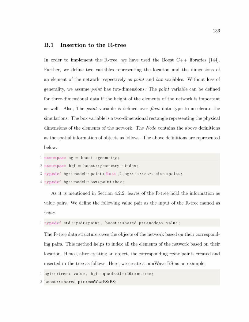
136
B.1 Insertion to the R-tree
In order to implement the R-tree, we have used the Boost C++ libraries [144].
Further, we define two variables representing the location and the dimensions of
an element of the network respectively as point and box variables. Without loss of
generality, we assume point has two-dimensions. The point variable can be defined
for three-dimensional data if the height of the elements of the network is important
as well. Also, The point variable is defined over float data type to accelerate the
simulations. The box variable is a two-dimensional rectangle representing the physical
dimensions of the elements of the network. The Node contains the above definitions
as the spatial information of objects as follows. The above definitions are represented
below.
1 namespace bg = boost : : geometry ;
2 namespace bgi = boost : : geometry : : index ;
3 typede f bg : : model : : point<f l o a t , 2 , bg : : c s : : c a r t e s i an>po int ;
4 typede f bg : : model : : box<point>box ;
As it is mentioned in Section 4.2.2, leaves of the R-tree hold the information as
value pairs. We define the following value pair as the input of the R-tree named as
value.
1 typede f std : : pa ir<point , boost : : shared ptr<node>> value ;
The R-tree data structure saves the objects of the network based on their correspond-
ing pairs. This method helps to index all the elements of the network based on their
location. Hence, after creating an object, the corresponding value pair is created and
inserted in the tree as follows. Here, we create a mmWave BS as an example.
1 bgi : : r t r e e< value , bg i : : quadrat ic<16>>m tree ;
2 boost : : shared ptr<mmWaveBS>BS ;

137
3 // Generate shared po in t e r o f a mmWaveBS
4 BS=boost : : shared ptr<mmWaveBS>(new mmWaveBS(x , y , get nextID ( ) , de f P tx ) ) ;
5 // I n s e r t the BS to the t r e e .
6 m tree . i n s e r t ( std : : make pair (BS−>g e t l o c ( ) ,BS) ) ;
In the first line above, the m tree is created as an R-tree over the defined value
pairs. The second and third line create a mmWaveBS and set its location, x, y,
identification number, and its transmit power. Finally, the created mmWaveBS is
inserted to the tree with its corresponding value in line four (The mmWaveBS contains
the get loc() method which returns the location of the object in point format.). Also,
since mmWaveBS is inherited from the Node, there is no need to cast it to the Node
object.
B.2 Parallel processing and message-passing
1. Parallel processing: In order to create a parallel process for an object inherited
from the TRX, the ThreadMain() method of the object should be implemented.
The desired functionality of the thread can be called from the Start method as
follows.
1 void Star t ( )
2 the thread=std : : thread(& des i r edObjec t : : ThreadMain , t h i s ) ;
In the above, a simple implementation of the Start method is presented. The
Start method calls the ThreadMain function as the main function of the thread.
2. Message-passing: Message-passing is implemented using simple signal-slot mech-
anisms. Any signal-slot mechanism contains three main fields, (i) the message
structure, (ii) the signal to be sent, and (iii) the destination function (slot).

138
You can connect functions to the signal which will be called when the emit()
method on the signal object is invoked. Any argument passed to emit() will be
passed to the given functions. For instance, for passing a message from object
O1 to a function in object O2, first we need to define the structure of the
message as follow.
1 s t r u c t Message char [ 2 0 ] s ; ;
In the above, the Message structure contains an array of characters. The signal
is defined in the sender, i.e., O1 as follow.
1 Signa l<Message const &> s i g n a l ;
and the function which handles the received message is defined in the O2 as
follows.
1 void handler ( Const Message& msg) ;
After ceating the objects O1 and O2, the signal and the slot are connected to
each other as follows.
1 s i g n a l . connect member(&O2, &O2 : : handler ) ;
In order to create an event or emit the signal, we just need to call the emit
function of the signal with the Message data as follows.
1 // Create the msg and F i l l in the f i e l d s .
2 Message msg ; msg . s = ” He l lo ! ”
3 // Emitting the msg .
4 s i g n a l . emit (msg) ;
By emitting the signal from the object O1, the handler function in the object
O2 receives the Message and is able to process it.

139
B.3 SINR characterization
In a randomly deployed network or a dynamic network where the active set of
transmitters and receivers change with time, deriving the set Ij (representing the
set of directional interferers) for the receiver j is challenging. However, with the
proposed architecture, any receiver can find the set Ij for any transmitter with the
defined queries in Section 4.2.3. In Algorithm 1, we illustrate how to calculate SINR
of the all possible mmWave links for a network containing a set N mmWave nodes.
Further, the code snippets of the Algorithm 1 is presented afterwards as well.
Algorithm 2 Evaluate SINR of all links in a mmWave network.
1: for j ∈ N do2: Retrieve desired level of the object j using dynamic cast3: Get position and ID of the node j.4: perform fixed-radius neighbor query to derive set Oj (Localizing the search)5: for i ∈ Oj do6: Retrieve desired level of the object i using dynamic cast7: Get position and ID of the node i.8: Derive the triangular polygon for the pair j and i9: Perform triangular query over the polygon to derive the set Ij
10: interference = 011: for k ∈ Ij do12: Calculate interference of node k and add it to interference13: end for14: Calculate SINRij
15: end for16: end for
1 // mmB i s the d e s i r e d r e c e i v e r SBS , c id and p1 are i t s ID and loca t i on ,
r e s p e c t i v e l y .
2 u i n t 3 2 t c id = mmB. get ( )−>getID ( ) ;
3 po int p1 = mmB−>g e t l o c ( ) ;
4 // search f o r f ixed−rad iu s nea r e s t ne ighbours r e s i d i n g in maximum mmWave
range .

140
5 std : : vector<value> r e s u l t s ;
6 m tree . query ( bgi : : s a t i s f i e s ( [ & ] ( va lue const& v ) re turn bg : : d i s t anc e ( v .
f i r s t , p1 ) < def MAX MMWAVE RANGE; ) , s td : : b a c k i n s e r t e r ( r e s u l t s ) ) ;
7 // Search in the r e s u l t e d SBSs in the maximum range .
8 BOOST FOREACH( value const&v , r e s u l t s )
9 bs p t r mmB2 = boost : : dynamic po inte r cas t<mmWaveBS>(v . second ) ;
10 u i n t 3 2 t c id2 = mmB2. get ( )−>getID ( ) ;
11 i f ( c id2 != c id )
12 double x2 = mmB2−>getX ( ) ; double y2 = mmB2−>getY ( ) ; po int p2 =
mmB2−>g e t l o c ( ) ;
13 // c r e a t e the i n t e r f e r e n c e t r i a n g u l a r polygon .
14 polygon2D poly = d i r e c t i o n a l p o l y g o n ( p1 , p2 , mmB−>get phi m ( ) ) ;
15 std : : vector<value> vec query ;
16 // Find the i n t e r f e r i n g SBSs .
17 m tree . query ( bgi : : i n t e r s e c t s ( poly ) , s td : : b a c k i n s e r t e r ( vec query
) ) ;
18 double i n t e r f =0. ;
19 BOOST FOREACH( value const&mz, vec query )
20 bs p t r mmB3 = boost : : dynamic po inter cas t<mmWaveBS>(mz .
second ) ;
21 u i n t 3 2 t c id3 = mmB3−>getID ( ) ;
22 i f ( c id3 != c id2 && cid3 != c id )
23 i n t e r f+= mmB−>c a l c u l a t e I n t e r f o f l i n k (mmB3−>getX ( ) ,
mmB3−>getY ( ) ) ;
24
25 // Ca lcu la te SNR and SINR of the l i n k .
26 double snr = mmB−>c a l c u l a t e S N R o f l i n k ( x2 , y2 ) ;
27 double s i n r = mmB−>c a l c u l a t e S I N R o f l i n k ( x2 , y2 , i n t e r f ) ;
28
29

141
Appendix C
CHAPTER 5

142
Figure C.1: Independent process of an agent and the main process.
C.1 Synchronous and Asynchronous Learning
Multi-agent RL, in its nature, is based on the interaction of each agent with the
environment. Hence, the agents can run their training algorithms separately. From a
computation standpoint, the independence of the training of each agent gives us the
opportunity to perform this task in parallel. Parallel training of the agents becomes
essential as the function approximator of each agent becomes expensive. For instance,
if each agent is using a deep neural network (DNN) as its function approximator
and backpropagation as the training algorithm, then parallel training and using all
resources is essential. Hence, we provide two methods of training for the RL agents,
(i) synchronous and (ii) asynchronous learning. In synchronous learning, agents are
trained in a queue by a single process. Synchronous learning can be used in simple

143
1 8 16 32
number of processors
0
10
20
30
40
50
60
70
80
90
Se
co
nds
1e5 iterations
1e6 iterations
Figure C.2: Running time for training of the WSN with 62 sensors. The running time forone process refers to synchronous learning and the rest are related to asynchronous learning.The machine specification for running the simulations is Intel(R) Xeon(R) CPU [email protected].
training algorithms or when the resources are limited. In asynchronous learning, each
agent runs its processes independently as a separate thread as in Fig. C.1. According
to Fig. C.1, an agent trains its own Q-function with a signal-slot structure. By
taking action a, the agent emits a signal containing its action. The environment as
the main thread receives this signal and runs the required processes to calculate the
reward and the new state of the agent. Meanwhile, the agent waits for the response
of the environment. The new state and the reward of the agent are emitted by the
environment. Upon receiving the new state and the reward, the agent updates its
Q-function, i.e., learning process, and then updates its state. Independent processes
for the agents bring scalability, which can be essential in large networks to use all the
computation resources.
Further, in order to investigate the scalability, we run the training process on

144
different machines with a different number of processes. Fig. C.2 presents the running
time of the training process for one, eight, 16, and 32 number of processes. Fig. C.2
shows the scalability of the simulator for using the existing resources to accelerate
the training processes. On the other hand, even for one processor, the running time
of the training is just 83.1 seconds for one million iterations. This result shows the
efficiency of the platform.