‘Love of Wealth’ and Economic Growth

Gunther Rehme∗

Technische Universitat Darmstadt†

September 2, 2016

Abstract

In a Ramsey-Cass-Koopmans growth framework it is shown that for an optimumthe social planner cannot have an excessive love of wealth. With a ‘right’ love ofwealth an optimum exists and implies higher long-run per capita capital, incomeand consumption relative to the standard model. This has important implica-tion for comparative development trajectories. The optimum implies dynamicefficiency with the possibility to get arbitrarily close to the Golden Rule wherelong-run per capita consumption is maximal. It is shown that the optimal pathis attaining its steady state more slowly. Thus, the beneficial effects of love ofwealth materialize later than in the standard model. Furthermore, the economycan be decentralized as a competitive private ownership economy. One can thenidentify love of wealth with the “spirit of capitalism”. The paper, hence, impliesthat one needs a ’right’ level of the “spirit of capitalism” to realize any beneficialeffects for the long run.

KEYWORDS: Economic Growth, Love of Wealth, Preference Shifts

JEL classification: O4, P0

∗I thank Sabine Eschenhof-Kammer and Steffen Roch for valuable help and comments. I havealso benefitted from feedback by Shesadri Banerjee, Michael Burda, Parantap Basu, Giacomo Corneo,Byeongju Jeong, Johanna Krenz, Alexander Meyer-Gohde, Sugata Gosh, Volker Grossmann, DanielNeuhoff, Yasuyuki Osumi, Simon Voigts, Lutz Weinke, Nikolaus Wolf, Xiaopeng Yin, Martin Zagler,as well as presentations at Humboldt University Berlin, the Royal Economic Society meeting in Cam-bridge, 2012, the Econometric Society European meeting in Gothenburg, the 9th Annual Conferenceon Economic Growth and Development, New Delhi, in 2013, the meetings of the Austrian (NOeG)and German (VfS) Economic Associations in Vienna and Hamburg in 2014, as well as the 2016 TaipeiInternational Conference on “Growth, Trade, and Dynamics” and the 2016 Asian Meeting of the Econo-metric Society in Kyoto.†Correspondence TU Darmstadt, Department of Economics, FB1/VWL1, Bleichstrasse 2, D-64283

Darmstadt, Germany. phone: +49-6151-16-57258; fax: +49-6151-16-57257; e-mail: rehme@vwl.tu-darmstadt.de

1 Introduction

It is generally recognized that people derive satisfaction from the holding of wealth.For instance, Weber (1930) and Pigou (1941) argue that individuals derive utility fromthe mere possession of wealth and not simply its expenditure.1 Clearly, putting wealthdirectly into the welfare (utility) function may allow to capture important and quiterealistic aspects of investment behaviour.2

Of course, investment behaviour is related to economic growth. In a seminal arti-cle Kurz (1968) has analyzed an optimal growth model in the spirit of Ramsey (1928),Cass (1965) and Koopmans (1965) where agents’ utility includes utility from holdingwealth. Keeping the analysis quite general Kurz shows that many different and com-plicated equilibria and transition dynamics may occur. Unfortunately, his paper doesnot present much economic intuition for his mathematical findings.

Simplified versions of his analysis were subsequently complemented by more eco-nomic interpretations. For example, Zou (1994), Bakshi and Chen (1996) and Carroll(2000) relate to Max Weber and argue that the dependence of utility on wealth capturesthe “spirit of capitalism”. Zou uses absolute, and Bakshi and Chen relative wealth intheir setups. In this paper I primarily relate to Zou’s optimal growth framework.

For the latter it is well known that the long-run equilibrium obeys the Modified

Golden Rule, under which the steady state capital stock is lower than the one associ-ated with the Golden Rule, derived by Phelps (1961), which would yield maximumlong-run, per capita consumption. Zou (1994) shows that utility derived from con-sumption and capital, where the latter is called love of wealth (LOW) in this paper,leads to an optimal path with a higher, steady state capital stock than under the Mod-ified Golden Rule.3 Corneo and Jeanne (1997) and Corneo and Jeanne (2001) showin an endogenous growth framework that love of (relative) wealth (“social status con-cerns” in their paper) can lead to an accumulation path that may even obey the GoldenRule. They also show that it is possible that too much love of wealth would entail over-

1For example, an early contribution that introduced wealth in the utility function in order to modelinvestment behaviour is Markowitz (1952). For recent papers that include love of wealth in their modelssee, for example, Kaplow (2009) and Kumhof and Ranciere (2010).

2One question is whether it is the relative wealth or the absolute wealth that enters utility. The formerallows to concentrate on status concerns, while the latter focuses on a form of ‘pure’ love of wealth.Both approaches can be found in the literature and I will relate to them below.

3The expression love of wealth, of course, draws on Plutarch’s (46 AD-120 AD) essay “Περιφιλoπλoυτ ιας” (“De Cupiditate Divitiarum” or “On the Love of Wealth”) in his Moralia that theinterested reader may wish to have a look at.

1

accumulation and would be socially undesirable. This is usually called “dynamicallyinefficient”.

Against this background the present paper derives complementary results. In orderto obtain those the paper concentrates on a simple logarithmic utility, Cobb-Douglastechnology economy with a social planner that derives utility from per capita wealthand consumption. Thus, the model builds on Ramsey (1928), Cass (1965) and Koop-mans (1965) who also analyze the problem of a central planning authority (social plan-ner).4 This makes it possible to get clean analytic expressions that serve to capture theessence of what love of wealth in a Solow (1956) growth context might imply. Theanalysis concentrates on steady states, but additionally on transitional dynamics whichsome earlier contributions have often not focussed on.5

In this context, the model yields the following results. There is no optimal accu-mulation path when there is excessive love of wealth. As the model’s social planneris taken to care about both per capita consumption and wealth, an excessive zeal foraccumulation would entail reductions in long-run consumption. Intuitively, the cravefor building ever more pyramids would have to be met with lower consumption in thelong run. As intuition suggests this is not a long-run optimum.

There exists a critical level of the love of wealth (LOW) below which optimal pathsexist. These paths are such that in a steady state per capita wealth and consumptionwould be higher than in an economy where there is no LOW. Thus, somewhat surpris-ingly, having the ‘right’ craving for capital also leads to higher long-run consumption.In that sense love of wealth is quite beneficial. It implies that a simple preference shiftfrom non-LOW to LOW allows for a better material situation, even for the consumers.However, in relative terms this is not so, because, even though the cake will be big-ger, the steady state consumption share will be lower, the investment share higher andthe return to capital lower in a LOW economy in comparison to the standard, optimalgrowth (non-LOW) economy.6

4Later in the paper we will look at the implication of the paper’s results for decentralized economies.The advantage to work with a social planner is that it may capture more general economic arrangements,of which a competitive decentralization is just one possibility.

5For instance, Wirl (1994) concentrates on transitional dynamics and the possibility of growth cy-cles when wealth enters utility. However, his paper concentrates rather on stability properties of sucheconomies. In the present paper the focus is more on steady state properties and the speed of conver-gence in relation to standard optimal growth models.

6Empirically this implies that economies may exhibit quite different long-run income levels in across section. According to the model this would be entirely due to preference and not technologydifferences.

2

In this model the LOW which implies optimal paths is always accompanied by “dy-namic efficiency”. In fact, (arbitrarily) close to the critical level of the love of wealth,the capital stock implied by the Golden Rule and that chosen by a social planner witha LOW near that critical level would be almost identical. The reason is that in a stan-dard optimal growth (non-LOW) model, impatience (the rate of time preference) issuch that a steady state capital stock is chosen that is less than the one that maximizessteady state consumption. Love of wealth provides a counteracting effect. Thus, it ispossible, even in a neoclassical, optimal growth context, to get arbitrarily close to theGolden Rule. Hence, the model implies some form of tradeoff between impatienceand love of wealth. Less patience can be compensated by more love of wealth if onewants to have the same level of steady state capital.

Next, by log-linearizing the economy with LOW preferences around its steady stateit is shown that the economy features saddle path stability. This is not too surprising,given the model’s structure. However, an interesting finding here is that convergence inan economy with LOW preferences occurs more slowly than in the standard non-LOWcase. Thus, two economies with these differences in preferences would converge dif-ferently to their respective steady states. The economy with LOW preferences wouldtake longer, but have a higher capital stock in the long run.7

This allows one to argue that transitions of economies can be seen as having beenstarted off by preference shifts. Suppose an economy without LOW preferences werein its steady state. Now assume that the social planner suddenly starts loving wealthand continues to do so forever. In a qualitative analysis using a phase diagram itturns out that taking the former steady state capital stock as the initial capital stockfor getting into the new equilibrium reveals the following quite intuitive results. Theeconomy will jump onto its new saddle path with lower consumption and higher in-vestment, compared to the previous regime with no LOW. So on impact consumerswill suffer as more investment is needed to obtain the new and higher steady state cap-ital stock associated with LOW preferences. There will be one point in time wherethe consumers will be just as well off as before the preference shift. After that dateconsumers will unambiguously benefit from the preference shift.

These results are interesting because they may contribute to explanations what mayhave happened in transition economies. Examples that may come to mind are theEastern European countries, Russia, China, India etc. For example, the model may

7To my knowledge of the literature this appears to be a novel finding. Of course, it holds only underthe assumptions made.

3

contribute to explanations why China, India and other economies have had such highinvestment rates over a longer period.

The logic of preference shifts towards capital might also apply to historical con-texts. Here the claim is that preference shifts, similar to those analyzed here, were atwork in the take-offs shortly before and during the Industrial Revolution. Of course,the model is too coarse to capture that in detail, but it may serve to highlight thepossibility of contemplating preference shifts as (perhaps additional) initial movers ofeconomic transitions.

Next, the paper invokes the second welfare theorem and argues that the contem-plated economy can be decentralized as a competitive general equilibrium of a privateownership economy. See, for example, Acemoglu (2009), ch. 5. Thus, the socialplanner solution can quite straightforwardly be turned into the outcome of a marketeconomy, given the assumptions about preferences and technology. This would re-quire that the agents would have to have the same preferences as the social plannercontemplated in this paper and where the social planner would have represented theagents’ welfare in a benevolent way. Thus, under these circumstances all the resultsunder the planner’s solution would also hold for the decentralized economy.

For the decentralized economy one may reasonably interpret the more general term“love of wealth” as representing the “spirit of capitalism” as in, for example, Zou(1994).8 Thus, for a competitive market economy we may then conclude that the‘right‘ level of the “spirit of capitalism” is good in terms of long-run income andconsumption. But it may take a little longer to realize these effects in comparison to aneconomy with less of that spirit. Furthermore, distinct (‘right’) “spirits of capitalism”may yield quite different economic outcomes in the long-run.9

However, one of the paper’s main insights is that an excessive “spirit of capitalism”is not optimal in that it cannot really be realized as a long-run optimum in a dynamiceconomy.

The paper is organized as follows. Sections 2 and 3 present the model and de-rive the social planner’s optimal decision rules. Sections 4 and 5 analyze the steadystate, and the transitional dynamics. Section 6 discusses decentralization, and section7 concludes.

8Notice that Zou contemplates a decentralized economy and sometimes uses a single, constant pa-rameter, as in the present paper, to represent the “spirit of capitalism”.

9That there are different forms of capitalism is, of course, well known. See, for example, Hall andSoskice (eds.) (2001).

4

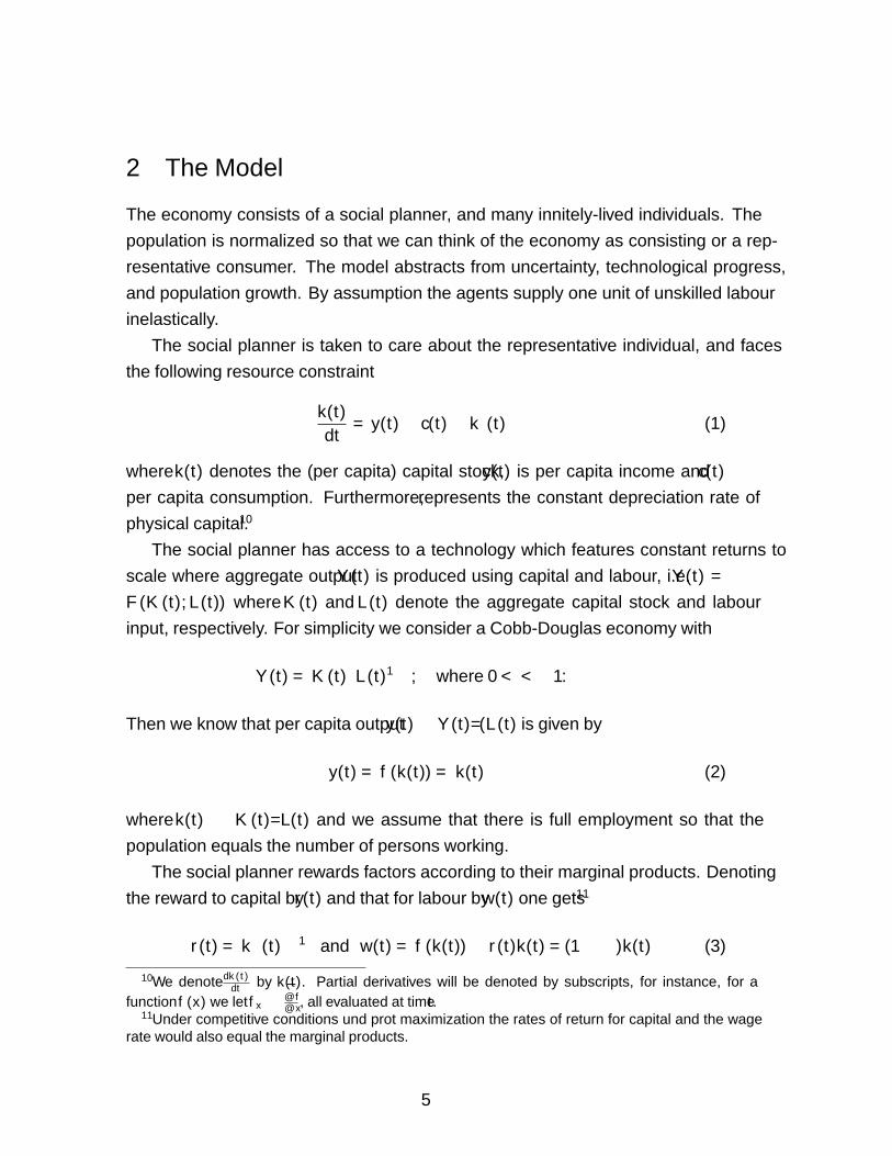
2 The Model

The economy consists of a social planner, and many infinitely-lived individuals. Thepopulation is normalized so that we can think of the economy as consisting or a rep-resentative consumer. The model abstracts from uncertainty, technological progress,and population growth. By assumption the agents supply one unit of unskilled labourinelastically.

The social planner is taken to care about the representative individual, and facesthe following resource constraint

k(t)

dt= y(t)− c(t)− δk(t) (1)

where k(t) denotes the (per capita) capital stock, y(t) is per capita income and c(t)per capita consumption. Furthermore, δ represents the constant depreciation rate ofphysical capital.10

The social planner has access to a technology which features constant returns toscale where aggregate output Y (t) is produced using capital and labour, i.e. Y (t) =

F (K(t), L(t)) where K(t) and L(t) denote the aggregate capital stock and labourinput, respectively. For simplicity we consider a Cobb-Douglas economy with

Y (t) = K(t)αL(t)1−α, where 0 < α < 1.

Then we know that per capita output y(t) ≡ Y (t)/(L(t) is given by

y(t) = f(k(t)) = k(t)α (2)

where k(t) ≡ K(t)/L(t) and we assume that there is full employment so that thepopulation equals the number of persons working.

The social planner rewards factors according to their marginal products. Denotingthe reward to capital by r(t) and that for labour by w(t) one gets11

r(t) = αk(t)α−1 and w(t) = f(k(t))− r(t)k(t) = (1− α)k(t)α (3)

10We denote dk(t)dt by ˙k(t). Partial derivatives will be denoted by subscripts, for instance, for a

function f(x) we let fx ≡ ∂f∂x , all evaluated at time t.

11Under competitive conditions und profit maximization the rates of return for capital and the wagerate would also equal the marginal products.

5

where the latter equality follows from the assumption of constant returns to scale.From now on I will drop the indication that variables depend on time for conve-

nience. When there may be cases where it needs to be made explicit, I will do so.

3 A Wealth-Loving Social Planner

Consider a social planner that maximizes an intertemporal utility stream subject tothe economy’s resource constraint in (1). The welfare stream for the social planner isgiven by ∫ ∞

0

u(c, k) e−ρtdt

where we assume the following for the period utility function u(·)

uc > 0, ucc < 0, uk > 0 and ukk < 0.

limc→0

uc =∞, limc→∞

uc = 0, limk→0

uk =∞ and limk→∞

uk = 0.

Thus, period utility depends in a conventional way on (per capita) consumptionc. What is different from usual problems is the fact that we assume that the socialplanner derives welfare from (per capita) wealth (capital).12 Thus, u(·) is a function ofk. This captures the fact that many people attach some value to wealth and capital perse. For instance, many people like to look at and visit impressive buildings (e.g. theEiffel Tower, or the Empire State Building etc.) and derive utility from that. Also,many firms offer guided tours through their often very impressive plants of productionsuch as e.g. the Boeing assembly halls in Seattle or Volkswagen’s “Auto Manufaktur”in Dresden.13

The assumption that welfare is increasing in wealth is perhaps more problematic.Clearly, there are cases where additional capital may be valued less. An example maybe the construction of an additional nuclear power plant. However, k is an index of all

12Notice there is a literature that makes preferences dependent on relative wealth. There is basicidea is that optimizers are comparing themselves with others. Here that most interesting question is nottaken up. Instead we focus on a planner that only looks at his or her own wealth. But this allows forcomparisons, too, because below we will conduct comparative static exercises by which one contrastsplanners with a higher and a lower preference for wealth.

13Clearly, marvelling at building from outside means that these buildings or plants have a public goodnature. However, visiting them usually requires a fee to be paid so that buildings and guided tours thenhave a private good nature.

6

sorts of capital stocks. Most evidence would suggest that people generally like wealthand especially more of it. Otherwise, they would not do the things one can observeto increase their wealth. Of course, this is a perennial phenomenon. Thus, drawingon this ‘stylized fact’ may justify the assumption that welfare is increasing in wealth,uk > 0.

The next assumption states that the marginal welfare of wealth is decreasing. Thus,the welfare gain becomes smaller as wealth increases. This may capture the observa-tion that very rich people often say that an additional “palazzo” may not make themmuch happier, especially in comparison to the first one they already call their own.

The Inada conditions on welfare’s reaction on the effects of wealth when there ishardly any or too much capital are not really necessary for most of the analysis below,but can be rationalized on quite intuitive grounds. For example, lim

k→0uk = ∞ would

say that one is really craving for wealth if one does not have any. Here the claim isthat many people would support that view. In turn, lim

k→∞uk = 0 would imply that Bill

Gates does not really care if he gets an additional computer.With all these assumptions the social planner’s problem really becomes

maxc

∫ ∞0

u(c, k) e−ρtdt

s.t. k = f(k)− c− δk; k0 > 0 and given.

A general problem of this kind is studied by Kurz (1968). He shows that many differenttrajectories may or may not lead to balanced growth paths. The potential solutions ofthis problem depend on the exact form of the period utility function u(c, k), and, inparticular, on the assumed substitution of consumption and capital in period utility.

In this paper one of the main questions that is being analyzed is how the steadystate and the speed of convergence are affected when moving from a regime wherethe social planner does not love capital to one where he or she does. To analyze thatquestion I will restrict the analysis to the log-utility case under the assumption that theperiod utility derived from capital and consumption are separable. Thus, it is assumedthat the social planner values each marginal increment of one component of utilityessentially independently of the increment of the other component. Thus, consider thefollowing period utility function

u(c, k) = ln c+ γ ln k where γ ∈ [0,∞). (4)

7

One easily verifies that this period utility function satisfies all the properties that themore general setup requires. Here γ measures the preference of the social planner forwealth (capital) in comparison to that for consumption. If γ = 0, the social plannerattaches no direct value to capital. If γ → ∞, the social planner is only concernedabout capital.

Thus, under the assumption of the period utility function in equation (4) the socialplanner’s problem is given by

maxc

∫ ∞0

[ln c+ γ ln k] e−ρtdt

s.t. k = f(k)− c− δk, k0 = given.(5)

where ρ represents the constant rate of time preference.The solution to this problem is obtained from the current value Hamiltonian

H = [ln c+ γ ln k] + λ [f(k)− c− δk]

and the first order necessary conditions for its maximization entail the following equa-tions have to be fulfilled

uc = λ (6)

λ = λρ− uk − λ(f ′ − δ) (7)

plus the requirement that the resource constraint in (1) and the transversality conditionlimt→∞

kλe−ρt = 0 be satisfied.14

Under the assumptions made equations (6) and (7) can then be rearranged to findthe social planner’s optimal consumption growth rate

c

c= f ′(k) + uk/uc − (ρ+ δ) = f ′(k) + γ · c

k− (ρ+ δ). (8)

Notice that, as is standard, consumption growth depends on the return to capital andthe rate of time preference. Additionally, in this model the marginal rate of substitution(in welfare) between consumption and wealth matters too. In our log-utility case thisis given by − dc

dk= uk

uc= γ · c

kand has a positive bearing on the (optimal) consumption

14One easily verifies that the Hamiltonian is concave in c and k so that by Mangasarian’s Theoremthe sufficient conditions for a maximum would also be be satisfied.

8

growth rate. Furthermore, we note that, if there is positive consumption growth, themarginal product will be lower than in a conventional optimal growth model, where itwould equal the sum of the depreciation and the time preference rate.

3.1 The transversality condition

The optimal consumption plan requires that the value of capital be zero at the end ofthe planning horizon. That imposes the requirement that

limt→∞

kt · λt · e−ρt = 0 (9)

hold. From equation (7) we know

λ = λ(−f ′ + (ρ+ δ))− γ

k.

Integrating this expression from time 0 up to time t yields

λt = e∫ t0 (ρ−f

′(kv)+δ)dv

(λ0 −

∫ t

0

(γ

ks

)e−

∫ s0 (ρ−f

′(kv)+δ)dvds

).

Inserting this into the transversality condition in (9) yields

limt→∞

kt · e∫ t0 (ρ−f

′(kv)+δ)dv

(λ0 −

∫ t

0

(γ

ks

)e−

∫ s0 (ρ−f

′(kv)+δ)dvds

)· e−ρt = 0.

as the condition to be satisfied. Noting that e∫ t0 ρdv = eρt we get

limt→∞

kt · e−∫ t0 (f′(kv)−δ)dv ·

(λ0 −

∫ t

0

(γ

ks

)e−

∫ s0 (ρ−f

′(kv)+δ)dvds

)= 0.

Clearly, this condition is equivalent to

limt→∞

kt · limt→∞

e−∫ t0 (f′(kv)−δ)dv ·

(λ0 − lim

t→∞

∫ t

0

(γ

ks

)e−

∫ s0 (ρ−f

′(kv)+δ)dvds

)= 0.

Jumping ahead it will turn out that in a long-run equilibrium limt→∞

kt = k∗ < ∞, thatis, the steady state capital stock k∗ will be finite. Then the product of the other limitsmust vanish asymptotically. With a finite capital stock in the long-run equilibrium thesecond limit requires lim

t→∞e−

∫ t0 (f′(kv)−δ)dv = 0 so that f ′(k∞) > δ in equilibrium is

9

needed and k∞ = k∗. See appendix A for more details. λ0 is a finite and positive num-ber. Thus, the product of λ0, the first and the second limit will be zero asymptotically,if f ′(k∗) > δ.

As regards the third limit it is shown in appendix A that the integral∫ ∞0

(γ

ks

)e−

∫ s0 (ρ−f

′(kv)+δ)dvds

converges to a finite number. Thus, the product of this and the other two limits will bezero asymptotically, if f ′(k∗) > δ, so that the transversality condition is indeed met.

Lemma 1 The transversality condition requires that f ′(k∗) > δ where k∗ denotes the

steady state capital stock.

As will be shown in more detail below, this is true in the steady state. The lemmahas the important implication that optimality requires that the social planner choose adynamically efficient solution.

4 The steady state

In the long-run, steady state equilibrium with balanced growth the economy is char-acterized by the condition k/k = c/c = 0. Using (1) and (8) for k/k = c/c requiresthat

f ′(k)− (ρ+ δ) + γc

k=

f(k)

k− c

k− δ

(γ + 1)c = f(k)− f ′(k) · k + ρk

c∗ = (w + ρk)

(1

γ + 1

)(10)

holds. Thus, consumption in steady state, c∗, depends on wage income and capitalincome net of investment outlays and on the welfare weight γ, which captures thepreference for capital. For given w, ρ and k, steady state consumption c∗ is decreasingin γ. This would suggest that a social planner that has a higher liking for capital wouldchoose accumulation such that steady state consumption is lower. However, higher γalso implies more capital in the steady state and that effect is captured by the followingarguments.

10

First notice that k = 0 implies that steady state consumption must also satisfy

c∗ = f(k)− δk. (11)

From this, i.e. equation (10) and (11) we can determine the steady state capital stockk∗ as satisfying

(f(k)− f ′(k) · k + ρ · k)) ·(

1

1 + γ

)= f(k)− δk

where, of course, w = f(k)− f ′(k) ·k. For our Cobb-Douglas economy we know thatf(k) = kα, and f ′(k) = αkα−1. Thus,

(1− α)kα−1 + ρ = (1 + γ)kα−1 − δ(1 + γ).

Then it is not difficult to verify that the steady state capital stock is given by

k∗ =

(α + γ

(γ + 1)δ + ρ

) 11−α

. (12)

and is increasing in γ. Thus, placing more welfare on capital holdings leads to ahigher capital stock in the steady state. This does not seem very surprising. From thisit follows that in an economy where there is a higher γ, the real return to capital in thesteady state will be lower.

As “love for wealth” affects c∗ through a direct and an indirect channel (through itseffect on k∗) it is interesting to know what the condition is so that more capital raisesoverall steady state consumption. Now c∗ = f(k∗)− δk∗ must hold in the steady state.Consumption c∗ changes with γ according to

dc∗

dγ= f ′(k∗) · ∂k

∗

∂γ− δ∂k

∗

∂γ.

We know that ∂k∗

∂γ> 0. Thus, the reaction of c∗ depends on

dc∗

dγR 0 iff f ′(k∗) R δ.

Lemma 2 If f ′(k∗) = δ, then steady state consumption would be maximized and the

“Golden Rule” of capital accumulation would be satisfied.

11

But from lemma 1 we know that the transversality condition requires f ′(k∗) > δ.Thus, this boils down to

f ′(k) = αk∗α−1 > δ that is,α[(γ + 1)δ + ρ]

α + γ> δ.

Simplification then reveals that γ has to satisfy

γ ≡ α

1− α· ρδ> γ. (13)

Thus, if this condition is satisfied consumption and the capital stock in the steadystate are higher than in an economy that does not feature love of wealth, i.e. whereγ = 0. Up to γ an increase in the love of wealth is accompanied by higher con-sumption and more physical capital in the steady state. Notice that the transversalitycondition requires that γ is smaller than γ. Interestingly, if γ equalled γ, then steadystate consumption would be maximized with respect to γ. One easily verifies that ifγ = γ, consumption would be maximal and the Golden Rule would hold. In this sim-ple model we would then get the textbook condition that the the marginal product ofcapital equals the depreciation rate.

In this context it is well known that the welfare discount factor (the time preferencerate ρ) leads one to choose a (steady state) consumption level that is smaller than themaximal one, i.e. the one that is associated with the Golden Rule. The reason isthat ρ also captures impatience and so it is optimal in a Ramsey model to consumemore today at the expense of higher consumption in the future. That implies a lowerlevel of steady state consumption. In this model it is found that love of wealth is acounteracting force. In the limit when the social planner would have a love of wealththat is extremely close to γ, the social optimum would be to pursue an accumulationpath that is almost equal to the one satisfying the Golden Rule.15

This holds, even if the the planner is more impatient. In this model more impatience(higher ρ) can be compensated in terms of steady state consumption by a higher γ aslong as γ > γ is satisfied.

Of course, higher consumption and more capital in the steady sate can only beaccomplished if the investment share is higher. Under the condition γ > γ, we find

15If γ is very close to γ one may then be unable to distinguish empirically between a simple Solowmodel with an exogenous savings rate that followed the Golden Rule, and a Ramsey model with en-dogenous savings decisions featuring time preference and love of wealth.

12

that the consumption share in steady state is

c∗

y∗=f(k∗)− δk∗

f(k∗)= 1− δk∗1−α where y = f(k∗) = k∗α,

which will be lower for an economy with a higher γ. Consequently, the long-runinvestment share is higher in an economy where there is love of wealth.

Proposition 1 More “love of wealth” (higher γ) increases the steady state capital

stock k∗ and implies a relatively lower steady state return to capital. It raises steady

state consumption c∗ if γ is not too large, that is, when γ < α1−α ·

ρδ≡ γ. If γ is very

close to, but still less than γ, the accumulation path will almost obey the Golden Rule.

However, if the love of wealth is too large (γ > γ), then an increase in γ would lower

steady state consumption c∗ in comparison to the maximum one, but then no optimum

exists. The social planner always chooses a dynamically efficient accumulation path in

the optimum. Furthermore, the optimal plan implies that an economy with more love

of wealth will have a lower consumption and a higher investment share in the steady

state.

The proposition is interesting for the following reasons. The social planner’s opti-mal policy is incompatible with an excessive love of wealth in the long run. A ’right’level of the love of wealth will lead to higher steady state consumption than when thereis no love of wealth. If γ were too large, then a social planner would overaccumulateat the expense of consumption. This is not viable as an equilibrium.16 A benevolentplanner with the ’right’ level of the love of wealth would not choose overaccumulationbecause she or he sees the potential for growth and higher consumption. By this rea-soning the ’right’ love of wealth is eventually beneficial for people and even though itimplies a lower consumption share in the steady state. Clearly, these features of themodel are in principle empirically testable. However, as the beneficial effect material-izes only in a new steady state when γ is raised from γ = 0, one has to analyze whathappens in the transition.

16In the most extreme case when γ → ∞, enslavement would ensue because the people wouldeventually die while producing more and consuming less, for example, by building ever more pyramids.

13

5 Transitional dynamics

For γ ∈ [0, αρ(1−α)δ ) the transitional dynamics of the economy can be described by the

following two-dimensional system.

k

k=f(k)

k− c

k− δ and

c

c= f ′(k)− (ρ+ δ) + γ

c

k

plus the initial condition k0 > 0 and the requirement that the transversality conditionis met. For our Cobb-Douglas production case with y = f(k) = kα and y′ = f ′(k) =

αkα−1 we then get for the equations of motion

k

k= kα−1 − c

k− δ and

c

c= αkα−1 − (ρ+ δ) + γ

c

k.

We will now log-linearize this system of equations around the steady state. Expressingthe last expression in (natural) logs yields

d ln kdt

= e−(1−α) ln k − eln(c/k) − δ (14)d ln cdt

= αe−(1−α) ln k + γeln(c/k) − (ρ+ δ). (15)

In steady state we have d ln kdt

= d ln cdt

= 0 so that

e−(1−α) ln k − eln(c/k) = δ (16)

αe−(1−α) ln k + γeln(c/k) = ρ+ δ (17)

have to hold. Solving for the steady state values yields

eln(c/k) = ρ+(1−α)δα+γ

(18)

e−(1−α) ln k = δ(1+γ)+ρα+γ

. (19)

Now we linearize (14) and (15) to get(d ln kdtd ln cdt

)= ∆ ·

(d ln k

d ln c

)

14

where d ln k = ln k − ln k∗ = ln(k/k∗) and d ln c = ln c− ln c∗ = ln(c/c∗) and

∆ ≡

(∆11 ∆12

∆21 ∆22

)≡

(−(1− α)e−(1−α) ln k + eln(c/k) −eln(c/k)

−α(1− α)e−(1−α) ln k − γeln(c/k) γeln(c/k)

)c∗, k∗

denotes the Jacobian of the system when in equilibrium. Evaluation at the steady stateyields after substitution of equations (18) and (19), rearrangement and simplificationthat17

∆11 = αρ−(1−α)γδα+γ

∆12 = −ρ+(1−α)δα+γ

∆21 = − 1α+γ· (α(1− α)[δ(1 + γ) + ρ] + γ[ρ+ (1− α)δ])

∆22 = γ(ρ+(1−α)δα+γ

) (20)

For the (local) stability analysis we can determine the characteristic equation which isgiven by∣∣∣∣∣∆11 − z ∆12

∆21 ∆22 − z

∣∣∣∣∣ = z2 − z(∆11 + ∆22) + ∆11∆22 −∆12∆21 = 0.

Notice that tr∆ = ∆11 + ∆22, which corresponds to the trace of the matrix ∆, and|∆| = ∆11∆22 −∆12∆21, which equals the determinant of ∆. The roots of the char-acteristic equation then satisfy

z1, z2 =tr∆±

√(tr∆)2 − 4|∆|

2(21)

where is it well-known that

z1 + z2 = tr∆ and z1z2 = |∆|.17∆ij was verified, and the determinant in (22) as well as the roots in (23) were

calculated in Mathematica 5.0. The source code is available in low-1-math.nb athttps://sites.google.com/site/rehmeguenther/resources/simulations-and-math-derivations/low2011.

15

Thus, the sum of the roots equals the trace of ∆ and the product of the roots equals itsdeterminant. In our case it is not difficult to, but cumbersome to derive that18

tr∆ = ρ and |∆| = −(a+ γ)−1 ((1− α)((1− α)δ + ρ)(δ(1 + γ) + ρ)) . (22)

This means that the product of the roots is negative. Hence, one root is positive andone is negative. Thus, the solution to the characteristic equation requires

2z = ρ±[ρ2 + 4(a+ γ)−1 ((1− α)((1− α)δ + ρ)(δ(1 + γ) + ρ))

]1/2 (23)

where z1, the root that takes the positive sign, is positive, and z2, the root that takes thenegative sign, is negative.

The log-linearized solution for ln k then boils down to

ln k = ln k∗ + ζ1 · ez1t + ζ2 · ez2t

where ζ1 and ζ2 are arbitrary constants of integration. As z1 > 0, we need that ζ1 = 0

for ln k to approach ln k∗ asymptotically. Then the other constant ζ2, the one that isassociated with z2 < 0, can be obtained from the initial condition ζ2 = ln k0− ln k∗.19

Thus, the evolution of k is described by

ln k = ln k∗ + [ln k0 − ln k∗] · ez2t, where z2 < 0.

As ln y = α ln k, one easily verifies that as a consequence output evolves according to

ln y = ln y∗ + [ln y0 − ln y∗] · ez2t, where z2 < 0.

It is well-known that the negative root z2 measures the speed of convergence. The lattertells one how fast the economy reaches its steady state. It is given by

2z2 = ρ−[ρ2 + 4(a+ γ)−1 ((1− α)((1− α)δ + ρ)(δ(1 + γ) + ρ))

]1/2.

18The details can be found at sites.google.com/site/rehmeguenther/resources/simulations-and-math-derivations/low2011.

19Here the assumption is that the initial values are close to the steady state. Although log-linearapproximations are widely used in macroeconomics, the requirement that they apply only as approxi-mations in the neighborhood of the steady sate can be regarded a disadvantage. See, for example, Barroand Sala–i–Martin (2004), p. 111.

16

If z2 is a large negative number then convergence takes place quickly. The oppositeholds for small negative values of z2. In appendix B it is shown that z2 is increasing inγ. Thus, a higher γ implies a less negative z2.

Proposition 2 An increase in the love of wealth is accompanied by a decrease in the

speed of convergence, that is, dz2dγ

> 0. Thus, an economy with love of wealth takes

longer to attain its steady state than an economy with no love of wealth.

The proposition is interesting because in a normal Cobb-Douglas economy withlogarithmic preferences and no love of wealth and a capital share of one third it isusually found that the convergence speed is too fast. See, for example, Barro andSala–i–Martin (2004), ch. 2. One way out of this problem has been to argue thatcapital should be broadly defined. With a higher value of α for broad capital, it canbe shown that the speed of convergence derived from a growth model with consumeroptimization can match the empirically observed convergence speeds. In that context,the present setup provides an alternative route by arguing that a larger love of wealthwould lead to a slower speed of convergence.

In order to see what the transitional dynamics of this system involve contemplatethe following. Suppose we compare an economy that features no love of wealth withone that does. In particular, assume that once an economy without love of wealth hasattained its steady state, the social planner will permanently change its preferencesand permanently loves wealth from the position onwards where there was no love ofwealth. Figure 1 displays the qualitative features of the dynamics if there is such apreferences shift. (The details of the phase diagram are derived in the appendix.)

17

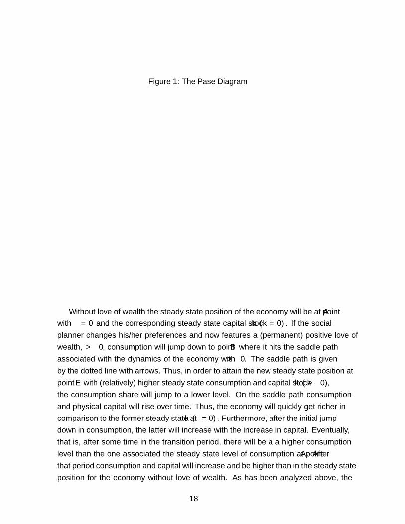
Figure 1: The Pase Diagram

)0(* =gk )0(* >gk

0=k&

k

A

B

I II

IV

c

E G

00 ==gc& 00 =>gc&

III

Without love of wealth the steady state position of the economy will be at point Awith γ = 0 and the corresponding steady state capital stock k∗(γ = 0). If the socialplanner changes his/her preferences and now features a (permanent) positive love ofwealth, γ > 0, consumption will jump down to point B where it hits the saddle pathassociated with the dynamics of the economy with γ > 0. The saddle path is givenby the dotted line with arrows. Thus, in order to attain the new steady state position atpoint E with (relatively) higher steady state consumption and capital stock k∗(γ > 0),the consumption share will jump to a lower level. On the saddle path consumptionand physical capital will rise over time. Thus, the economy will quickly get richer incomparison to the former steady state at k∗(γ = 0). Furthermore, after the initial jumpdown in consumption, the latter will increase with the increase in capital. Eventually,that is, after some time in the transition period, there will be a a higher consumptionlevel than the one associated the steady state level of consumption at point A. Afterthat period consumption and capital will increase and be higher than in the steady stateposition for the economy without love of wealth. As has been analyzed above, the

18

economy will end up in a new steady state that has higher capital, consumption andincome than in the economy without love of wealth.

6 Decentralization

The setup of the model is such that a convex economy is analyzed. The utility functionand the technology are (quasi)concave functions of its arguments. One can then invokethe Second Welfare Theorem and argue that the planner solution can be decentralizedas a competitive general equilibrium of a private ownership economy. See Debreu(1959), Mas-Colell, Whinston, and Green (1995), ch. 16, and, more related to ourgrowth context, Acemoglu (2009), ch. 5. Thus, the social planner solution can berealized as a market economy. This would only require that the agents have the samepreferences as the social planner and where the social planner would have representedthe agents’ welfare in a benevolent way. Thus, all the results derived from the planner’ssolution would also carry over to the decentralized economy.

For the decentralized economy one can then interpret the more general term “loveof wealth” as representing the “spirit of capitalism” as done in, for example, Zou(1994).20 Thus, for a competitive market economy we may then conclude that the‘right‘ level of the “spirit of capitalism” is good in terms of long-run income and con-sumption. But it may take a little longer to realize these effects in comparison to aneconomy with less of that spirit. Furthermore, distinct (‘right’) “spirits of capitalism”may yield quite different economic outcomes in the long-run.

However, one main insight that the model can capture is that an excessive “spirit ofcapitalism” is not optimal, in the sense that it cannot really be realized as a long-runoptimum in a dynamic economy.

7 Conclusion

In a simple optimal growth framework with Cobb-Douglas production technology andlogarithmic utility which includes wealth as an argument it is analyzed how ‘love ofwealth’ bears on optimal paths in a Solovian growth setup from a social planner’sperspective. The following findings of the paper are noteworthy.

20Notice that Zou contemplates a decentralized economy and also sometimes uses a single, constantvalue to represent the “spirit of capitalism”.

19

First, for excessive ‘love of wealth’ no optimum exists for the social planner. If theintensity of the ‘love of wealth’ is ’right’, i.e. below some critical threshold, there willbe an equilibrium with higher per capita income, consumption and capital in compar-ison to the standard Ramsey-Cass-Koopmans world. In this case ‘love of wealth’ willdefinitely be beneficial for the agents and the social planner. In particular, long-run percapita consumption will be higher.

Second, with ‘love of wealth’ it is in principle possible to get arbitrarily close to theGolden Rule level of long-run consumption. The optimum implies that a dynamicallyefficient path will be followed and no overaccumulation will take place. There is atradeoff between the rate of time preference (impatience) and the model’s indicator ofthe ‘love of wealth’. More impatience implies a lower and a higher intensity of the‘love of wealth’ a higher steady state capital stock.

Third, an economy in which ‘love of wealth’ features in the preferences will havea slower speed of convergence. Thus, in comparison to the standard model it willtake such an economy longer to attain its steady state. In a transition from a standardRamsey-Cass-Koopmans economy to one that starts to like wealth from some point intime onwards and maintains this liking, it will take some time to realize the eventualbenefits of having higher consumption and wealth. So initially some agents will notbenefit, but from some time onwards they will.

Fourth, the social planner optimum can be decentralized as a private ownership,competitive economy. Building on previous work one may then identify ’love ofwealth’ with the “spirit of capitalism”. All the results would then carry over for thedecentralized economy. An important implication of the formal model then is that, assometimes argued in recent policy debates on the virtues and vices of capitalism, anexcessive “spirit of capitalism” precludes an optimum. In turn, a ’right’ spirit will bequite beneficial for the long run.

The present paper should really be viewed as an additional move in the directionof focussing more on the role of preferences in accumulation processes. Of course, theanalysis faces several caveats. The setup of the model is simple. Alternative utility andproduction functions might imply far more complicated equilibria or the lack thereof.’Love of wealth’ was captured by a constant. This begs the question how changes overtime in the ’love of wealth’ may bear on the optimal paths. These and other extensionsof the model are left for further research.

20

A Proof of the transversality condition

First, it is shown that limt→∞

e−∫ t0 (f′(kv)−δ)dv = 0 requires f ′(k∞) > δ where k∞ = k∗ and k∗

denotes the finite steady state capital stock.

Suppose the economy starts off with some initial capital stock k0 < k∗. At some point

in time, called v∗, we will have k0 < kv∗ < k∗. By assumption f ′(k) is a smooth and

decreasing function of k. If f ′(k∗) > δ, then it must be that f ′(kv) > δ and f ′(k0) > δ.

Thus, −∫ t0 (f ′(kv) − δ)dv will be a negative number. Taking the limit one easily verifies that

limt→∞

e−∫ t0 (f′(kv)−δ)dv = 0 if f ′(k∗) > δ and k0 < kv∗ < k∗.

Suppose the economy starts off with some initial capital stock k0 > k∗ so that k0 > kv∗ >

k∗. Then it is true that

−∫ t

0(f ′(kv)− δ)dv = −

∫ v∗

0(f ′(kv)− δ)dv −

∫ t

v∗(f ′(kv)− δ)dv (24)

Starting from a large k0, we have f ′(k0) < δ. Thus, the expression in first integral on the right

hand side will be a positive, but finite number, as the upper limit of integration is finite and

f ′(k) is a monotone function. Thus,

−∫ v∗

0(f ′(kv)− δ)dv = c0

where c0 is a positive constant which is independent of t. Given that f ′(k) is a decreasing

function of k and as we consider k approaching k∗ from k0 > k∗ there will be some time v∗

with k0 > kv∗ > k∗ where f ′(kv∗) > δ.

Now the second integral on the right hand side is equivalent to

−∫ t

v∗(f ′(kv)− δ)dv = −t

(∫ tv∗(f

′(kv)dv

t

)+ δ(t− v∗).

Taking the limit yields

− limt→∞

t · limt→∞

(∫ tv∗(f

′(kv)dv

t

)+ limt→∞

δ(t− v∗).

Using l’Hopital’s Rule one then finds

− limt→∞

t · f ′(k∞) + limt→∞

δ(t− v∗) = − limt→∞

(f ′(k∞)− δ)t− δv∗ = −∞

because f ′(k∞) > δ and k∗ = k∞. Hence, if f ′(k∗) > δ, then limt→∞

e−∫ t0 (f′(kv)−δ)dv = 0.

21

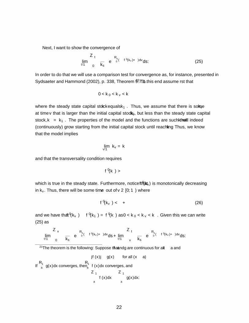
Next, I want to show the convergence of

limt→∞

∫ t

0

(γ

ks

)e−

∫ s0 (ρ−f

′(kv)+δ)dvds. (25)

In order to do that we will use a comparison test for convergence as, for instance, presented in

Sydsaeter and Hammond (2002), p. 338, Theorem 9.7.1.21 To this end assume first that

0 < k0 < kv < k∗

where the steady state capital stock k∗ equals k∞. Thus, we assume that there is some kvat time v that is larger than the initial capital stock, k0, but less than the steady state capital

stock, k∗ = k∞. The properties of the model and the functions are such that k will indeed

(continuously) grow starting from the initial capital stock until reaching k∗. Thus, we know

that the model implies

limv→∞

kv = k∗

and that the transversality condition requires

f ′(k∗) > δ

which is true in the steady state. Furthermore, notice that f ′(kv) is monotonically decreasing

in kv. Thus, there will be some time v∗ out of v ∈ [0,∞) where

f ′(kv∗) < δ + ρ (26)

and we have that f ′(kv∗) ≥ f ′(k∞) = f ′(k∗) as 0 < k0 < kv < k∗. Given this we can write

(25) as

limt→∞

∫ v∗

0

(γ

ks

)e−

∫ s0 (ρ−f

′(kv)+δ)dvds+ limt→∞

∫ t

v∗

(γ

ks

)e−

∫ s0 (ρ−f

′(kv)+δ)dvds.

21The theorem is the following: Suppose that f and g are continuous for all x ≥ a and

|f(x)| ≤ g(x) for all (x ≥ a)

If∫∞ag(x)dx converges, then

∫∞af(x)dx converges, and∣∣∣∣∫ ∞a

f(x)dx

∣∣∣∣ ≤ ∫ ∞a

g(x)dx.

22

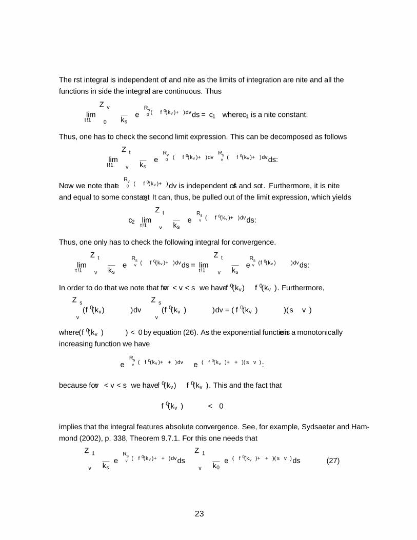
The first integral is independent of t and finite as the limits of integration are finite and all the

functions in side the integral are continuous. Thus

limt→∞

∫ v∗

0

(γ

ks

)e−

∫ s0 (ρ−f

′(kv)+δ)dvds = c1 where c1 is a finite constant.

Thus, one has to check the second limit expression. This can be decomposed as follows

limt→∞

∫ t

v∗

(γ

ks

)e−

∫ v∗0 (ρ−f ′(kv)+δ)dv−

∫ sv∗ (ρ−f

′(kv)+δ)dvds.

Now we note that e−∫ v∗0 (ρ−f ′(kv)+δ)dv is independent of s and so t. Furthermore, it is finite

and equal to some constant c2. It can, thus, be pulled out of the limit expression, which yields

c2 · limt→∞

∫ t

v∗

(γ

ks

)e−

∫ sv∗ (ρ−f

′(kv)+δ)dvds.

Thus, one only has to check the following integral for convergence.

limt→∞

∫ t

v∗

(γ

ks

)e−

∫ sv∗ (ρ−f

′(kv)+δ)dvds = limt→∞

∫ t

v∗

(γ

ks

)e∫ sv∗ (f

′(kv)−ρ−δ)dvds.

In order to do that we note that for v∗ < v < s we have f ′(kv) ≤ f ′(kv∗). Furthermore,∫ s

v∗(f ′(kv)− ρ− δ)dv ≤

∫ s

v∗(f ′(kv∗)− ρ− δ)dv = (f ′(kv∗)− ρ− δ)(s− v∗)

where (f ′(kv∗)−ρ−δ) < 0 by equation (26). As the exponential function e is a monotonically

increasing function we have

e−∫ sv∗ (−f

′(kv)+ρ+δ)dv ≤ e−(−f ′(kv∗ )+ρ+δ)(s−v∗).

because for v∗ < v < s we have f ′(kv) ≤ f ′(kv∗). This and the fact that

f ′(kv∗)− ρ− δ < 0

implies that the integral features absolute convergence. See, for example, Sydsaeter and Ham-

mond (2002), p. 338, Theorem 9.7.1. For this one needs that∫ ∞v∗

∣∣∣∣ γks∣∣∣∣ e− ∫ s

v∗ (−f′(kv)+ρ+δ)dvds ≤

∫ ∞v∗

∣∣∣∣ γk0∣∣∣∣ e−(−f ′(kv∗ )+ρ+δ)(s−v∗)ds (27)

23

The integral on the right hand side is given by∣∣∣∣ γk0∣∣∣∣ · e(−f ′(kv∗ )+ρ+δ)v∗ · ∫ ∞

v∗e−(−f

′(kv∗ )+ρ+δ)sds, (28)

where the expression in front of the integral is a constant. The integral, in turn, is of the type∫ ∞v∗

e−asds, where a = (ρ+ δ − f ′(kv∗)) > 0. (29)

Then it is not difficult to verify that∫ ∞v∗

e−asds = limt→∞

∫ t

v∗e−asds = lim

t→∞

e−as

−a

∣∣∣∣tv∗

= limt→∞

1

−a

(e−at − e−av∗

)=e−av

∗

a<∞.

Thus, the integral on the right hand side of equation (27) converges. But by the comparison

test for convergence it must then be that the integral on the left hand side of equation (27)

converges, which in turn implies that

limt→∞

e−∫ t0 (f′(kv)−δ)dv · lim

t→∞

∫ t

0

(γ

ks

)e−

∫ s0 (ρ−f

′(kv)+δ)dvds = 0. (30)

This follows from the arguments above and in the text.

Finally it remains to check if the integral (25) converges if we approach the steady state

from the right, that is, from

∞ > k0 > kv > k∗.

It is not difficult to see that then−∫ s0 (ρ−f ′(kv)+δ)dv will be a negative number in that case.

Going through essentially the same steps as before it is not difficult to see that∫ ∞v∗

∣∣∣∣ γks∣∣∣∣ e− ∫ s

v∗ (−f′(kv)+ρ+δ)dvds ≤

∫ ∞v∗

∣∣∣ γk∗

∣∣∣ e−(−f ′(kv∗ )+ρ+δ)(s−v∗)ds (31)

is needed for convergence. The integral on the right hand side of the inequality is convergent.

Hence that (25) also converges if we start from k0 > k∗

Together with the arguments in the main text, it then follows that the transversality condi-

tion is indeed met if f ′(k∗) > δ and f ′(k∗) < δ + ρ which is true in the steady state.

24

B Proof that the convergence speed is decreasing in γ

The negative root is given by

2z2 = ρ−[ρ2 + 4(a+ γ)−1 ((1− α)((1− α)δ + ρ)(δ(1 + γ) + ρ))

]1/2.

This equation can be rearranged as

ρ2 + 4(α+ γ)−1 (∆(δ(1 + γ) + ρ)) = (ρ− 2z2)2 where ∆ ≡ ((1− α)((1− α)δ + ρ).

Taking the differential with respect to z2 and γ yields

(−4(α+ γ)−2∆(δ(1 + γ) + ρ) + 4(α+ γ)−1δ∆

)dγ = (−2)(ρ− 2z2)dz2

4(α+ γ)−1∆[−(α+ γ)−1(δ(1 + γ) + ρ) + δ

]dγ = (−2)(ρ− 2z2)dz2.

The expression in brackets is negative, because negativity requires

δ(α+ γ) < δ(1 + γ) + γ

δα < δ + γ

which is true as δα < δ. For the right hand side notice that, as z2 < 0, the expression (ρ−2z2)

is positive. thus, it follows that z2 is increasing in γ, i.e. dz2/dγ > 0. Thus, a higher γ implies

a lower speed of convergence.

C The phase diagram

The qualitative features of the dynamic system are characterized as follows. The system of

differential equations is

k

k= kα−1 − c

k− δ and

c

c= αkα−1 − (ρ+ δ) + γ

c

k.

When k = 0 in the steady state we get c = kα − δk. Taking the differential with respect to k

and c yields

dc = (αkα−1 − δ)dk.

As the expression in the round brackets is positive for low k and negative for sufficiently large

k, the (k = 0)-line will be inverted U-shaped as depicted in figure 1. This is a standard result.

25

When c = 0 we get γc = (ρ+ δ)k−αkα. Taking the differential for this expression yields

γ · dc =((ρ+ δ)− α2kα−1

)dk. (32)

This means that dcdk |c=0

< 0 for very low k and dcdk |c=0

> 0 for sufficiently large k. For the

arguments in the text initial k for the preference shift corresponds to the one where k∗ is not a

function of γ. The latter is given by

k∗|γ=0 =

(α

δ + ρ

) 11−α

. (33)

But then it is easy to verify that dcdk |c=0

> 0 holds for any k > k∗|γ=0. Starting from k∗|γ=0 it

also turns out that d2cdk2 |c=0

> 0 so that the (c = 0)-line is a convex function of k as depicted in

figure 1.

Turning to the dynamic adjustment notice that

dk

dc= −1. (34)

Thus, if c is slightly above the (k = 0)-line, k will fall. That explains the arrows pointing

westward above that line. Similarly, if c is slightly below the (k = 0)-line, k will rise, which

explains the arrows pointing eastward above the (k = 0)-line.

As concerns the (c = 0)-line notice that

dc =[α(α− 1)kα−2 − γ c

k2

]c · dk.

The expression in square brackets is negative. Thus, dcdk |c=0< 0. So if k is to the right of the

(c = 0)-line, consumption decreases. That explains the downward pointing arrows on the right

of the (c = 0)-line. Furthermore, if k is to the left of the (c = 0)-line, consumption increases.

That explains the upward pointing arrows on the left of the (c = 0)-line.

26

ReferencesACEMOGLU, D. (2009): Introduction to Modern Economic Growth. Princeton University

Press, Princeton, New Jersey.

BAKSHI, G. S., AND Z. CHEN (1996): “The Spirit of Capitalism and Stock-Market Prices,”American Economic Review, 86, 133–157.

BARRO, R. J., AND X. SALA–I–MARTIN (2004): Economic Growth. MIT Press, Cambridge,Massachusetts, 2nd edn.

CARROLL, C. D. (2000): “Why Do the Rich Save So Much?,” in Does Atlas Shrug? TheEconomic Consequences of Taxing the Rich, ed. by J. B. Slemrod, pp. 465–484. RusselSage Foudation and Harvard University Press, New York and Cambridge, Mass.

CASS, D. (1965): “Optimum Growth in an Aggregative Model of Capital Accumulation,”Review of Economic Studies, 32, 233–240.

CORNEO, G., AND O. JEANNE (1997): “On relative wealth effects and the optimality ofgrowth,” Economics Letters, 54, 87–92.

(2001): “Status, the Distribution of Wealth, and Growth,” Scandinavian Journal ofEconomics, 103, 283–293.

DEBREU, G. (1959): Theory of Value. Wiley, New York.

HALL, P., AND D. SOSKICE (EDS.) (2001): Varieties of Capitalism. The Institutional Foun-dations of Comparative Advantage. Oxford University Press, Oxford, United Kingdom, 1stedn.

KAPLOW, L. (2009): “Utility From Accumulation,” Working Paper 15595, NBER, Cambridge,MA.

KOOPMANS, T. C. (1965): “On the Concept of Optimal Growth,” in The Econometric Ap-proach to Development Planning. North Holland, Amsterdam.

KUMHOF, M., AND R. RANCIERE (2010): “Inequality, Leverage and Crises,” Working PaperWP/10/268, International Monetary Fund, Washington, DC.

KURZ, M. (1968): “Optimal Economic Growth and Wealth Effects,” International EconomicReview, 9, 348–357.

MARKOWITZ, H. (1952): “The Utility of Wealth,” Journal of Political Economy, LX, 151–158.

MAS-COLELL, A., M. D. WHINSTON, AND J. R. GREEN (1995): Microeconomic Theory.Oxford University Press.

PHELPS, E. (1961): “The Golden Rule of Accumulation: A Fable for Growthmen,” AmericanEconomic Review, 51, 638–643.

27

PIGOU, A. C. (1941): Employment and Equilibrium: A Theoretical Discussion. Maxmillan,London.

RAMSEY, F. P. (1928): “A Mathematical Theory of Saving,” Economic Journal, 38, 543–559.

SOLOW, R. M. (1956): “A Contribution to the Theory of Economic Growth,” Quarterly Jour-nal of Economics, 70(1), 65–94.

SYDSAETER, K., AND P. HAMMOND (2002): Essential Mathematics for Economic Analysis.Prentice Hall, Harlow, England, 1st edn.

WEBER, M. (1930): The Protestant Ethic and the Spirit of Capitalism. Allen & Unwin, Lon-don, transl. by talcott parsons edn.

WIRL, F. (1994): “The Ramsey Model Revisited: The Optimality of Cyclical Consumptionand Growth,” Journal of Economics, 60, 81–98.

ZOU, H. (1994): “The spirit of capitalism’ and long-run growth,” European Journal of PoliticalEconomy, 10, 279–293.

28