regularized principal component analysis for spatial data
TRANSCRIPT

.
.
.
.
.
.
.
.
.
.
.
.
.
.
.
.
.
.
.
.
.
.
.
.
.
.
.
.
.
.
.
.
.
.
.
.
.
.
.
.
Regularized Principal Component Analysis forSpatial Data
Wen-Ting Wang
Institute of Statistics, National Chiao Tung University
January 25, 2017
Joint work with Hsin-Cheng Huang, Academia Sinica
1

.
.
.
.
.
.
.
.
.
.
.
.
.
.
.
.
.
.
.
.
.
.
.
.
.
.
.
.
.
.
.
.
.
.
.
.
.
.
.
.
Background Regularized Principal Component Analysis Computation algorithm Numerical Example Summary
Outline
1 Background
2 Regularized Principal Component Analysis
3 Computation algorithm
4 Numerical Example
5 Summary
2

.
.
.
.
.
.
.
.
.
.
.
.
.
.
.
.
.
.
.
.
.
.
.
.
.
.
.
.
.
.
.
.
.
.
.
.
.
.
.
.
Background Regularized Principal Component Analysis Computation algorithm Numerical Example Summary
Outline
1 Background
2 Regularized Principal Component Analysis
3 Computation algorithm
4 Numerical Example
5 Summary
3

.
.
.
.
.
.
.
.
.
.
.
.
.
.
.
.
.
.
.
.
.
.
.
.
.
.
.
.
.
.
.
.
.
.
.
.
.
.
.
.
Background Regularized Principal Component Analysis Computation algorithm Numerical Example Summary
Background• Spatial processes of interest:
ηi(s); s ∈ D ; i = 1, . . . , n
– D ⊂ Rd
– mean zero– common covariance function: Cη(s
∗, s) = Cov(ηi(s∗), ηi(s))– η1(·), . . . , ηn(·): uncorrelated
• Observed data at locations s1, . . . , sp ∈ D,
Yi(sj) = ηi(sj) + ϵij; i = 1, . . . , n, j = 1, . . . , p
– ϵij ∼ (0, σ2): white noise– ϵij and ηi(sj) are uncorrelated for any i, j
4

.
.
.
.
.
.
.
.
.
.
.
.
.
.
.
.
.
.
.
.
.
.
.
.
.
.
.
.
.
.
.
.
.
.
.
.
.
.
.
.
Background Regularized Principal Component Analysis Computation algorithm Numerical Example Summary
Targets
1 Detect the dominant patterns (modes) of η1(·), . . . , ηn(·)– interpret the variability of spatial data physically
2 Estimate spatial covariance function Cη(·, ·)– no specific assumption (e.g., parametric form or stationarity)
– spatial prediction (kriging) of ηi(s); s ∈ D
5

.
.
.
.
.
.
.
.
.
.
.
.
.
.
.
.
.
.
.
.
.
.
.
.
.
.
.
.
.
.
.
.
.
.
.
.
.
.
.
.
Background Regularized Principal Component Analysis Computation algorithm Numerical Example Summary
Example: dominant patterns
• Two dominant patterns (Deser, 2009)Basin-wide mode East-west dipole mode
−0.04 −0.02 0.00 0.02 0.04
– Data: Indian Ocean sea surface temperature anomalies (Monthly average)– related to El Ninõ–Southern Oscillation (ENSO)
6

.
.
.
.
.
.
.
.
.
.
.
.
.
.
.
.
.
.
.
.
.
.
.
.
.
.
.
.
.
.
.
.
.
.
.
.
.
.
.
.
Background Regularized Principal Component Analysis Computation algorithm Numerical Example Summary
Rank-K spatial model• Data:
Yi(sj) = ηi(sj)
K∑k=1
ξik
+ ϵij ; i = 1, . . . , n, j = 1 . . . , p
– ξi1, . . . , ξiK∼ (0,Λ); ΛK×K is positive-definite– φ1(·) . . . , φK(·): K unknown orthonormal functions– ξik uncorrelated with ϵij
• Spatial covariance function:
Cη(s∗, s) =
K∑k=1
K∑k′=1
λkk′φk(s∗)φk′(s)
– λkk′ : (k, k′) entry of Λ
7

.
.
.
.
.
.
.
.
.
.
.
.
.
.
.
.
.
.
.
.
.
.
.
.
.
.
.
.
.
.
.
.
.
.
.
.
.
.
.
.
Background Regularized Principal Component Analysis Computation algorithm Numerical Example Summary
Rank-K spatial model• Data:
Yi(sj) =
K∑k=1
ξikφk(sj) + ϵij ; i = 1, . . . , n, j = 1 . . . , p
– ξi1, . . . , ξiK∼ (0,Λ); ΛK×K is positive-definite– φ1(·) . . . , φK(·): K unknown orthonormal functions– ξik uncorrelated with ϵij
• Spatial covariance function:
Cη(s∗, s) =
K∑k=1
K∑k′=1
λkk′φk(s∗)φk′(s)
– λkk′ : (k, k′) entry of Λ
8

.
.
.
.
.
.
.
.
.
.
.
.
.
.
.
.
.
.
.
.
.
.
.
.
.
.
.
.
.
.
.
.
.
.
.
.
.
.
.
.
Background Regularized Principal Component Analysis Computation algorithm Numerical Example Summary
Goal
• Find φ1(·), . . . , φK(·) to represent the dominant patterns.
• Standard approach: Principal component analysis (PCA)
9

.
.
.
.
.
.
.
.
.
.
.
.
.
.
.
.
.
.
.
.
.
.
.
.
.
.
.
.
.
.
.
.
.
.
.
.
.
.
.
.
Background Regularized Principal Component Analysis Computation algorithm Numerical Example Summary
Principal Component Analysis
• p-dimensional data vector:
Yi = (Yi(s1), . . . , Yi(sp))′ ∼ (0,Σ)
• Idea: Find ϕ ∈ Rp with ϕ′ϕ = 1,which maximizes Var(ϕ′Yi)
• Spectral decomposition: Σ– eigenvalues: λ1 ≥ · · · ≥ λp
– eigenvectors: ϕ1, . . . ,ϕp
• Dominant patterns: ϕ1, . . . ,ϕK (with λ1, . . . , λK large)
10

.
.
.
.
.
.
.
.
.
.
.
.
.
.
.
.
.
.
.
.
.
.
.
.
.
.
.
.
.
.
.
.
.
.
.
.
.
.
.
.
Background Regularized Principal Component Analysis Computation algorithm Numerical Example Summary
Principal Component Analysis
• Data matrix: Yn×p = (Y1, . . . ,Yn)′
• Sample covariance matrix: S = Y ′Y /n
• Spectral decomposition: S– sample eigenvalues: λ1 ≥ · · · ≥ λp
– sample eigenvectors: ϕ1, . . . , ϕp
• ϕ1, . . . , ϕK are estimates of ϕ1, . . . ,ϕK
• Problems:– high estimation variability: n is small or p is large
→ unstable and noisy patterns→ weak physical interpretation
– without spatial structure of ϕ
11

.
.
.
.
.
.
.
.
.
.
.
.
.
.
.
.
.
.
.
.
.
.
.
.
.
.
.
.
.
.
.
.
.
.
.
.
.
.
.
.
Background Regularized Principal Component Analysis Computation algorithm Numerical Example Summary
Principal Component Analysis
• Data matrix: Yn×p = (Y1, . . . ,Yn)′
• Sample covariance matrix: S = Y ′Y /n
• Spectral decomposition: S– sample eigenvalues: λ1 ≥ · · · ≥ λp
– sample eigenvectors: ϕ1, . . . , ϕp
• ϕ1, . . . , ϕK are estimates of ϕ1, . . . ,ϕK
• Problems:– high estimation variability: n is small or p is large
→ unstable and noisy patterns→ weak physical interpretation
– without spatial structure of ϕ
11
.
.
.
.
.
.
.
.
.
.
.
.
.
.
.
.
.
.
.
.
.
.
.
.
.
.
.
.
.
.
.
.
.
.
.
.
.
.
.
.
Background Regularized Principal Component Analysis Computation algorithm Numerical Example Summary
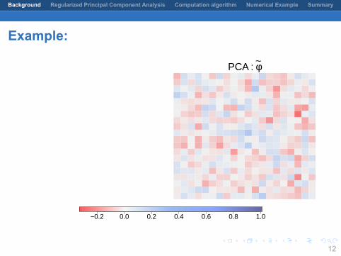
Example:
True : φ
PCA : φ~
−0.2 0.0 0.2 0.4 0.6 0.8 1.0
12

.
.
.
.
.
.
.
.
.
.
.
.
.
.
.
.
.
.
.
.
.
.
.
.
.
.
.
.
.
.
.
.
.
.
.
.
.
.
.
.
Background Regularized Principal Component Analysis Computation algorithm Numerical Example Summary
Example:
True : φ PCA : φ~
−0.2 0.0 0.2 0.4 0.6 0.8 1.0
12

.
.
.
.
.
.
.
.
.
.
.
.
.
.
.
.
.
.
.
.
.
.
.
.
.
.
.
.
.
.
.
.
.
.
.
.
.
.
.
.
Background Regularized Principal Component Analysis Computation algorithm Numerical Example Summary
Motivation
To enhance the interpretablity, we implement PCA by incorporating
1 spatial structure of eigenvectors2 sparsity of eigenvectors3 orthogonality of eigenvectors
13

.
.
.
.
.
.
.
.
.
.
.
.
.
.
.
.
.
.
.
.
.
.
.
.
.
.
.
.
.
.
.
.
.
.
.
.
.
.
.
.
Background Regularized Principal Component Analysis Computation algorithm Numerical Example Summary
Motivation
To enhance the interpretablity, we implement PCA by incorporating1 spatial structure of eigenvectors
2 sparsity of eigenvectors3 orthogonality of eigenvectors
13

.
.
.
.
.
.
.
.
.
.
.
.
.
.
.
.
.
.
.
.
.
.
.
.
.
.
.
.
.
.
.
.
.
.
.
.
.
.
.
.
Background Regularized Principal Component Analysis Computation algorithm Numerical Example Summary
Motivation
To enhance the interpretablity, we implement PCA by incorporating1 spatial structure of eigenvectors2 sparsity of eigenvectors
3 orthogonality of eigenvectors
13

.
.
.
.
.
.
.
.
.
.
.
.
.
.
.
.
.
.
.
.
.
.
.
.
.
.
.
.
.
.
.
.
.
.
.
.
.
.
.
.
Background Regularized Principal Component Analysis Computation algorithm Numerical Example Summary
Motivation
To enhance the interpretablity, we implement PCA by incorporating1 spatial structure of eigenvectors2 sparsity of eigenvectors3 orthogonality of eigenvectors
13

.
.
.
.
.
.
.
.
.
.
.
.
.
.
.
.
.
.
.
.
.
.
.
.
.
.
.
.
.
.
.
.
.
.
.
.
.
.
.
.
Background Regularized Principal Component Analysis Computation algorithm Numerical Example Summary
Outline
1 Background
2 Regularized Principal Component Analysis
3 Computation algorithm
4 Numerical Example
5 Summary
14

.
.
.
.
.
.
.
.
.
.
.
.
.
.
.
.
.
.
.
.
.
.
.
.
.
.
.
.
.
.
.
.
.
.
.
.
.
.
.
.
Background Regularized Principal Component Analysis Computation algorithm Numerical Example Summary
Quick review• Data Yi = (Yi(s1), . . . , Yi(sp))
′; i = 1, . . . , n
– Yi(sj) =K∑
k=1
ξikφk(sj) + ϵij ; j = 1 . . . , p
• φ1(·) . . . , φK(·): K unknown orthonormal functions• ξi1, . . . , ξiK∼ (0,Λ); ΛK×K ≻ 0• ϵij ∼ (0, σ2); ϵij : uncorrelated with ξik
• Spatial covariance function:
Cη(s∗, s) =
K∑k=1
K∑k′=1
λkk′φk(s∗)φk′(s)
– λkk′ : (k, k′) entry of Λ
• Unknown parameters: φ1(·), . . . , φK(·), Λ, σ2
15

.
.
.
.
.
.
.
.
.
.
.
.
.
.
.
.
.
.
.
.
.
.
.
.
.
.
.
.
.
.
.
.
.
.
.
.
.
.
.
.
Background Regularized Principal Component Analysis Computation algorithm Numerical Example Summary
PCA (alternative version)
• Data matrix: Yn×p = (Y1, . . . ,Yn)′
• PCA :Φ = argmin
Φ:Φ′Φ=IK
∥Y − Y ΦΦ′∥2F
– Φp×K = (ϕ1, . . . ,ϕK) with ϕjk = φj(sk)
– ∥M∥2F =
n∑i=1
p∑j=1
m2ij
16

.
.
.
.
.
.
.
.
.
.
.
.
.
.
.
.
.
.
.
.
.
.
.
.
.
.
.
.
.
.
.
.
.
.
.
.
.
.
.
.
Background Regularized Principal Component Analysis Computation algorithm Numerical Example Summary
Regularized PCA• Data matrix: Yn×p = (Y1, . . . ,Yn)
′
• Φp×K = (ϕ1, . . . ,ϕK) with ϕjk = φj(sk)
• Objective function
∥Y − Y ΦΦ′∥2F
+τ1
K∑k=1
J(φk) + τ2
K∑k=1
p∑j=1
|φk(sj)|
subject to Φ′Φ = IK
– J(φk) =∑
z1+···+zd=2
∫Rd
(∂2φk(s)
∂xz11 . . . ∂x
zdd
)2
ds
• s = (x1, . . . , xd)′
– τ1: smoothness parameter
– τ2: sparseness parameter
17

.
.
.
.
.
.
.
.
.
.
.
.
.
.
.
.
.
.
.
.
.
.
.
.
.
.
.
.
.
.
.
.
.
.
.
.
.
.
.
.
Background Regularized Principal Component Analysis Computation algorithm Numerical Example Summary
Regularized PCA• Data matrix: Yn×p = (Y1, . . . ,Yn)
′
• Φp×K = (ϕ1, . . . ,ϕK)
with ϕjk = φj(sk)
• Objective function
∥Y − Y ΦΦ′∥2F+τ1
K∑k=1
J(φk) + τ2
K∑k=1
p∑j=1
|φk(sj)|
subject to Φ′Φ = IK
– J(φk) =∑
z1+···+zd=2
∫Rd
(∂2φk(s)
∂xz11 . . . ∂x
zdd
)2
ds
• s = (x1, . . . , xd)′
– τ1: smoothness parameter
– τ2: sparseness parameter
17

.
.
.
.
.
.
.
.
.
.
.
.
.
.
.
.
.
.
.
.
.
.
.
.
.
.
.
.
.
.
.
.
.
.
.
.
.
.
.
.
Background Regularized Principal Component Analysis Computation algorithm Numerical Example Summary
Spatial PCA (SpatPCA)
• J(φk) = ϕ′kΩϕk
– Ωp×p: determined only by s1, . . . , sp
– Ref: Green and Silverman (1994)
• Proposal: SpatPCA
Φ = argminΦ:Φ′Φ=IK
∥Y − Y ΦΦ′∥2F + τ1
K∑k=1
ϕ′kΩϕk + τ2
K∑k=1
p∑j=1
|ϕjk|
• As τ1 = τ2 = 0, ϕk is the k-th eigenvector of S.
18

.
.
.
.
.
.
.
.
.
.
.
.
.
.
.
.
.
.
.
.
.
.
.
.
.
.
.
.
.
.
.
.
.
.
.
.
.
.
.
.
Background Regularized Principal Component Analysis Computation algorithm Numerical Example Summary
SpatPCA: φ1(·), . . . , φK(·)• (φ1(·), . . . , φK(·)) minimizes
∥Y − Y ΦΦ′∥2F+τ1
K∑k=1
J(φk) + τ2
K∑k=1
p∑j=1
|φk(sj)|,
subject to Φ′Φ = IK• φk(·): smoothing spline based on ϕk
φk(s) =
p∑i=1
aig(∥s− si∥) + b0 +
d∑j=1
bjxj
– s = (x1, . . . , xd)′
– g(r) =
1
16πr2 log r; if d = 2,
Γ(d/2− 2)
16πd/2r4−d; if d = 1, 3,
– a = (a1, . . . , ap)′ and b = (b0, b1, . . . , bd)
′ depend on ϕk
19

.
.
.
.
.
.
.
.
.
.
.
.
.
.
.
.
.
.
.
.
.
.
.
.
.
.
.
.
.
.
.
.
.
.
.
.
.
.
.
.
Background Regularized Principal Component Analysis Computation algorithm Numerical Example Summary
Why considering two penalties?
20

.
.
.
.
.
.
.
.
.
.
.
.
.
.
.
.
.
.
.
.
.
.
.
.
.
.
.
.
.
.
.
.
.
.
.
.
.
.
.
.
Background Regularized Principal Component Analysis Computation algorithm Numerical Example Summary
1D Example
τ1 = 0True PCA SpatPCA
21

.
.
.
.
.
.
.
.
.
.
.
.
.
.
.
.
.
.
.
.
.
.
.
.
.
.
.
.
.
.
.
.
.
.
.
.
.
.
.
.
Background Regularized Principal Component Analysis Computation algorithm Numerical Example Summary
Case 1: ϕ as τ2 = 0 (only smoothness)
τ1 = 0True PCA SpatPCA
22

.
.
.
.
.
.
.
.
.
.
.
.
.
.
.
.
.
.
.
.
.
.
.
.
.
.
.
.
.
.
.
.
.
.
.
.
.
.
.
.
Background Regularized Principal Component Analysis Computation algorithm Numerical Example Summary
Case 1: ϕ as τ2 = 0 (only smoothness)
τ1 = 0.03True PCA SpatPCA
23

.
.
.
.
.
.
.
.
.
.
.
.
.
.
.
.
.
.
.
.
.
.
.
.
.
.
.
.
.
.
.
.
.
.
.
.
.
.
.
.
Background Regularized Principal Component Analysis Computation algorithm Numerical Example Summary
Case 1: ϕ as τ2 = 0 (only smoothness)
τ1 = 0.09True PCA SpatPCA
24

.
.
.
.
.
.
.
.
.
.
.
.
.
.
.
.
.
.
.
.
.
.
.
.
.
.
.
.
.
.
.
.
.
.
.
.
.
.
.
.
Background Regularized Principal Component Analysis Computation algorithm Numerical Example Summary
Case 1: ϕ as τ2 = 0 (only smoothness)
τ1 = 0.32True PCA SpatPCA
25

.
.
.
.
.
.
.
.
.
.
.
.
.
.
.
.
.
.
.
.
.
.
.
.
.
.
.
.
.
.
.
.
.
.
.
.
.
.
.
.
Background Regularized Principal Component Analysis Computation algorithm Numerical Example Summary
Case 1: ϕ as τ2 = 0 (only smoothness)
τ1 = 3.81True PCA SpatPCA
26

.
.
.
.
.
.
.
.
.
.
.
.
.
.
.
.
.
.
.
.
.
.
.
.
.
.
.
.
.
.
.
.
.
.
.
.
.
.
.
.
Background Regularized Principal Component Analysis Computation algorithm Numerical Example Summary
Case 1: ϕ as τ2 = 0 (only smoothness)
τ1 = 156.17True PCA SpatPCA
27

.
.
.
.
.
.
.
.
.
.
.
.
.
.
.
.
.
.
.
.
.
.
.
.
.
.
.
.
.
.
.
.
.
.
.
.
.
.
.
.
Background Regularized Principal Component Analysis Computation algorithm Numerical Example Summary
Case 1: ϕ as τ2 = 0 (only smoothness)
τ1 = 6405.22True PCA SpatPCA
28

.
.
.
.
.
.
.
.
.
.
.
.
.
.
.
.
.
.
.
.
.
.
.
.
.
.
.
.
.
.
.
.
.
.
.
.
.
.
.
.
Background Regularized Principal Component Analysis Computation algorithm Numerical Example Summary
Case 1: ϕ as τ2 = 0 (only smoothness)
τ1 = 25000True PCA SpatPCA
29

.
.
.
.
.
.
.
.
.
.
.
.
.
.
.
.
.
.
.
.
.
.
.
.
.
.
.
.
.
.
.
.
.
.
.
.
.
.
.
.
Background Regularized Principal Component Analysis Computation algorithm Numerical Example Summary
Case 2: ϕ as τ1 = 0 (only sparseness)
τ2 = 0True PCA SpatPCA
30

.
.
.
.
.
.
.
.
.
.
.
.
.
.
.
.
.
.
.
.
.
.
.
.
.
.
.
.
.
.
.
.
.
.
.
.
.
.
.
.
Background Regularized Principal Component Analysis Computation algorithm Numerical Example Summary
Case 2: ϕ as τ1 = 0 (only sparseness)
τ2 = 39True PCA SpatPCA
31
.
.
.
.
.
.
.
.
.
.
.
.
.
.
.
.
.
.
.
.
.
.
.
.
.
.
.
.
.
.
.
.
.
.
.
.
.
.
.
.
Background Regularized Principal Component Analysis Computation algorithm Numerical Example Summary
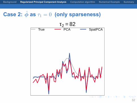
Case 2: ϕ as τ1 = 0 (only sparseness)
τ2 = 82True PCA SpatPCA
32

.
.
.
.
.
.
.
.
.
.
.
.
.
.
.
.
.
.
.
.
.
.
.
.
.
.
.
.
.
.
.
.
.
.
.
.
.
.
.
.
Background Regularized Principal Component Analysis Computation algorithm Numerical Example Summary
Case 2: ϕ as τ1 = 0 (only sparseness)
τ2 = 126True PCA SpatPCA
33

.
.
.
.
.
.
.
.
.
.
.
.
.
.
.
.
.
.
.
.
.
.
.
.
.
.
.
.
.
.
.
.
.
.
.
.
.
.
.
.
Background Regularized Principal Component Analysis Computation algorithm Numerical Example Summary
Case 2: ϕ as τ1 = 0 (only sparseness)
τ2 = 212True PCA SpatPCA
34

.
.
.
.
.
.
.
.
.
.
.
.
.
.
.
.
.
.
.
.
.
.
.
.
.
.
.
.
.
.
.
.
.
.
.
.
.
.
.
.
Background Regularized Principal Component Analysis Computation algorithm Numerical Example Summary
Case 2: ϕ as τ1 = 0 (only sparseness)
τ2 = 342True PCA SpatPCA
35

.
.
.
.
.
.
.
.
.
.
.
.
.
.
.
.
.
.
.
.
.
.
.
.
.
.
.
.
.
.
.
.
.
.
.
.
.
.
.
.
Background Regularized Principal Component Analysis Computation algorithm Numerical Example Summary
Case 2: ϕ as τ1 = 0 (only sparseness)
τ2 = 472True PCA SpatPCA
36

.
.
.
.
.
.
.
.
.
.
.
.
.
.
.
.
.
.
.
.
.
.
.
.
.
.
.
.
.
.
.
.
.
.
.
.
.
.
.
.
Background Regularized Principal Component Analysis Computation algorithm Numerical Example Summary
Case 2: ϕ as τ1 = 0 (only sparseness)
τ2 = 520True PCA SpatPCA
37

.
.
.
.
.
.
.
.
.
.
.
.
.
.
.
.
.
.
.
.
.
.
.
.
.
.
.
.
.
.
.
.
.
.
.
.
.
.
.
.
Background Regularized Principal Component Analysis Computation algorithm Numerical Example Summary
Case 3: ϕ as τ1 = τ2
τ1 = τ2 = 0True PCA SpatPCA
38

.
.
.
.
.
.
.
.
.
.
.
.
.
.
.
.
.
.
.
.
.
.
.
.
.
.
.
.
.
.
.
.
.
.
.
.
.
.
.
.
Background Regularized Principal Component Analysis Computation algorithm Numerical Example Summary
Case 3: ϕ as τ1 = τ2
τ1 = τ2 = 0.02True PCA SpatPCA
39

.
.
.
.
.
.
.
.
.
.
.
.
.
.
.
.
.
.
.
.
.
.
.
.
.
.
.
.
.
.
.
.
.
.
.
.
.
.
.
.
Background Regularized Principal Component Analysis Computation algorithm Numerical Example Summary
Case 3: ϕ as τ1 = τ2
τ1 = τ2 = 0.04True PCA SpatPCA
40
.
.
.
.
.
.
.
.
.
.
.
.
.
.
.
.
.
.
.
.
.
.
.
.
.
.
.
.
.
.
.
.
.
.
.
.
.
.
.
.
Background Regularized Principal Component Analysis Computation algorithm Numerical Example Summary
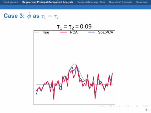
Case 3: ϕ as τ1 = τ2
τ1 = τ2 = 0.09True PCA SpatPCA
41

.
.
.
.
.
.
.
.
.
.
.
.
.
.
.
.
.
.
.
.
.
.
.
.
.
.
.
.
.
.
.
.
.
.
.
.
.
.
.
.
Background Regularized Principal Component Analysis Computation algorithm Numerical Example Summary
Case 3: ϕ as τ1 = τ2
τ1 = τ2 = 0.41True PCA SpatPCA
42

.
.
.
.
.
.
.
.
.
.
.
.
.
.
.
.
.
.
.
.
.
.
.
.
.
.
.
.
.
.
.
.
.
.
.
.
.
.
.
.
Background Regularized Principal Component Analysis Computation algorithm Numerical Example Summary
Case 3: ϕ as τ1 = τ2
τ1 = τ2 = 4.19True PCA SpatPCA
43

.
.
.
.
.
.
.
.
.
.
.
.
.
.
.
.
.
.
.
.
.
.
.
.
.
.
.
.
.
.
.
.
.
.
.
.
.
.
.
.
Background Regularized Principal Component Analysis Computation algorithm Numerical Example Summary
Case 3: ϕ as τ1 = τ2
τ1 = τ2 = 42.68True PCA SpatPCA
44

.
.
.
.
.
.
.
.
.
.
.
.
.
.
.
.
.
.
.
.
.
.
.
.
.
.
.
.
.
.
.
.
.
.
.
.
.
.
.
.
Background Regularized Principal Component Analysis Computation algorithm Numerical Example Summary
Case 3: ϕ as τ1 = τ2
τ1 = τ2 = 100True PCA SpatPCA
45

.
.
.
.
.
.
.
.
.
.
.
.
.
.
.
.
.
.
.
.
.
.
.
.
.
.
.
.
.
.
.
.
.
.
.
.
.
.
.
.
Background Regularized Principal Component Analysis Computation algorithm Numerical Example Summary
2D Example
True : φ PCA : φ~
−0.2 0.0 0.2 0.4 0.6 0.8 1.0
46

.
.
.
.
.
.
.
.
.
.
.
.
.
.
.
.
.
.
.
.
.
.
.
.
.
.
.
.
.
.
.
.
.
.
.
.
.
.
.
.
Background Regularized Principal Component Analysis Computation algorithm Numerical Example Summary
Case 1: ϕ as τ2 = 0 (only smoothness)
True : φ τ1 = 0
−0.2 0.0 0.2 0.4 0.6 0.8 1.0
47

.
.
.
.
.
.
.
.
.
.
.
.
.
.
.
.
.
.
.
.
.
.
.
.
.
.
.
.
.
.
.
.
.
.
.
.
.
.
.
.
Background Regularized Principal Component Analysis Computation algorithm Numerical Example Summary
Case 1: ϕ as τ2 = 0 (only smoothness)
True : φ τ1 = 0
−0.2 0.0 0.2 0.4 0.6 0.8 1.0
48

.
.
.
.
.
.
.
.
.
.
.
.
.
.
.
.
.
.
.
.
.
.
.
.
.
.
.
.
.
.
.
.
.
.
.
.
.
.
.
.
Background Regularized Principal Component Analysis Computation algorithm Numerical Example Summary
Case 1: ϕ as τ2 = 0 (only smoothness)
True : φ τ1 = 93
−0.2 0.0 0.2 0.4 0.6 0.8 1.0
49
.
.
.
.
.
.
.
.
.
.
.
.
.
.
.
.
.
.
.
.
.
.
.
.
.
.
.
.
.
.
.
.
.
.
.
.
.
.
.
.
Background Regularized Principal Component Analysis Computation algorithm Numerical Example Summary
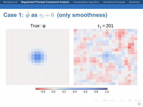
Case 1: ϕ as τ2 = 0 (only smoothness)
True : φ τ1 = 201
−0.2 0.0 0.2 0.4 0.6 0.8 1.0
50

.
.
.
.
.
.
.
.
.
.
.
.
.
.
.
.
.
.
.
.
.
.
.
.
.
.
.
.
.
.
.
.
.
.
.
.
.
.
.
.
Background Regularized Principal Component Analysis Computation algorithm Numerical Example Summary
Case 1: ϕ as τ2 = 0 (only smoothness)
True : φ τ1 = 437
−0.2 0.0 0.2 0.4 0.6 0.8 1.0
51

.
.
.
.
.
.
.
.
.
.
.
.
.
.
.
.
.
.
.
.
.
.
.
.
.
.
.
.
.
.
.
.
.
.
.
.
.
.
.
.
Background Regularized Principal Component Analysis Computation algorithm Numerical Example Summary
Case 1: ϕ as τ2 = 0 (only smoothness)
True : φ τ1 = 2053
−0.2 0.0 0.2 0.4 0.6 0.8 1.0
52

.
.
.
.
.
.
.
.
.
.
.
.
.
.
.
.
.
.
.
.
.
.
.
.
.
.
.
.
.
.
.
.
.
.
.
.
.
.
.
.
Background Regularized Principal Component Analysis Computation algorithm Numerical Example Summary
Case 1: ϕ as τ2 = 0 (only smoothness)
True : φ τ1 = 20932
−0.2 0.0 0.2 0.4 0.6 0.8 1.0
53

.
.
.
.
.
.
.
.
.
.
.
.
.
.
.
.
.
.
.
.
.
.
.
.
.
.
.
.
.
.
.
.
.
.
.
.
.
.
.
.
Background Regularized Principal Component Analysis Computation algorithm Numerical Example Summary
Case 1: ϕ as τ2 = 0 (only smoothness)
True : φ τ1 = 213414
−0.2 0.0 0.2 0.4 0.6 0.8 1.0
54

.
.
.
.
.
.
.
.
.
.
.
.
.
.
.
.
.
.
.
.
.
.
.
.
.
.
.
.
.
.
.
.
.
.
.
.
.
.
.
.
Background Regularized Principal Component Analysis Computation algorithm Numerical Example Summary
Case 1: ϕ as τ2 = 0 (only smoothness)
True : φ τ1 = 5e+05
−0.2 0.0 0.2 0.4 0.6 0.8 1.0
55

.
.
.
.
.
.
.
.
.
.
.
.
.
.
.
.
.
.
.
.
.
.
.
.
.
.
.
.
.
.
.
.
.
.
.
.
.
.
.
.
Background Regularized Principal Component Analysis Computation algorithm Numerical Example Summary
Case 2: ϕ as τ2 = 0 (only sparseness)
True : φ τ2 = 0
−0.2 0.0 0.2 0.4 0.6 0.8 1.0
56

.
.
.
.
.
.
.
.
.
.
.
.
.
.
.
.
.
.
.
.
.
.
.
.
.
.
.
.
.
.
.
.
.
.
.
.
.
.
.
.
Background Regularized Principal Component Analysis Computation algorithm Numerical Example Summary
Case 2: ϕ as τ2 = 0 (only sparseness)
True : φ τ2 = 35
−0.2 0.0 0.2 0.4 0.6 0.8 1.0
57

.
.
.
.
.
.
.
.
.
.
.
.
.
.
.
.
.
.
.
.
.
.
.
.
.
.
.
.
.
.
.
.
.
.
.
.
.
.
.
.
Background Regularized Principal Component Analysis Computation algorithm Numerical Example Summary
Case 2: ϕ as τ2 = 0 (only sparseness)
True : φ τ2 = 42
−0.2 0.0 0.2 0.4 0.6 0.8 1.0
58

.
.
.
.
.
.
.
.
.
.
.
.
.
.
.
.
.
.
.
.
.
.
.
.
.
.
.
.
.
.
.
.
.
.
.
.
.
.
.
.
Background Regularized Principal Component Analysis Computation algorithm Numerical Example Summary
Case 2: ϕ as τ2 = 0 (only sparseness)
True : φ τ2 = 50
−0.2 0.0 0.2 0.4 0.6 0.8 1.0
59

.
.
.
.
.
.
.
.
.
.
.
.
.
.
.
.
.
.
.
.
.
.
.
.
.
.
.
.
.
.
.
.
.
.
.
.
.
.
.
.
Background Regularized Principal Component Analysis Computation algorithm Numerical Example Summary
Case 2: ϕ as τ2 = 0 (only sparseness)
True : φ τ2 = 73
−0.2 0.0 0.2 0.4 0.6 0.8 1.0
60

.
.
.
.
.
.
.
.
.
.
.
.
.
.
.
.
.
.
.
.
.
.
.
.
.
.
.
.
.
.
.
.
.
.
.
.
.
.
.
.
Background Regularized Principal Component Analysis Computation algorithm Numerical Example Summary
Case 2: ϕ as τ2 = 0 (only sparseness)
True : φ τ2 = 127
−0.2 0.0 0.2 0.4 0.6 0.8 1.0
61

.
.
.
.
.
.
.
.
.
.
.
.
.
.
.
.
.
.
.
.
.
.
.
.
.
.
.
.
.
.
.
.
.
.
.
.
.
.
.
.
Background Regularized Principal Component Analysis Computation algorithm Numerical Example Summary
Case 2: ϕ as τ2 = 0 (only sparseness)
True : φ τ2 = 220
−0.2 0.0 0.2 0.4 0.6 0.8 1.0
62

.
.
.
.
.
.
.
.
.
.
.
.
.
.
.
.
.
.
.
.
.
.
.
.
.
.
.
.
.
.
.
.
.
.
.
.
.
.
.
.
Background Regularized Principal Component Analysis Computation algorithm Numerical Example Summary
Case 2: ϕ as τ2 = 0 (only sparseness)
True : φ τ2 = 270
−0.2 0.0 0.2 0.4 0.6 0.8 1.0
63

.
.
.
.
.
.
.
.
.
.
.
.
.
.
.
.
.
.
.
.
.
.
.
.
.
.
.
.
.
.
.
.
.
.
.
.
.
.
.
.
Background Regularized Principal Component Analysis Computation algorithm Numerical Example Summary
Case 3: ϕ as τ1 = τ2
True : φ τ1 = τ2 = 0
−0.2 0.0 0.2 0.4 0.6 0.8 1.0
64

.
.
.
.
.
.
.
.
.
.
.
.
.
.
.
.
.
.
.
.
.
.
.
.
.
.
.
.
.
.
.
.
.
.
.
.
.
.
.
.
Background Regularized Principal Component Analysis Computation algorithm Numerical Example Summary
Case 3: ϕ as τ1 = τ2
True : φ τ1 = τ2 = 33
−0.2 0.0 0.2 0.4 0.6 0.8 1.0
65

.
.
.
.
.
.
.
.
.
.
.
.
.
.
.
.
.
.
.
.
.
.
.
.
.
.
.
.
.
.
.
.
.
.
.
.
.
.
.
.
Background Regularized Principal Component Analysis Computation algorithm Numerical Example Summary
Case 3: ϕ as τ1 = τ2
True : φ τ1 = τ2 = 38
−0.2 0.0 0.2 0.4 0.6 0.8 1.0
66

.
.
.
.
.
.
.
.
.
.
.
.
.
.
.
.
.
.
.
.
.
.
.
.
.
.
.
.
.
.
.
.
.
.
.
.
.
.
.
.
Background Regularized Principal Component Analysis Computation algorithm Numerical Example Summary
Case 3: ϕ as τ1 = τ2
True : φ τ1 = τ2 = 43
−0.2 0.0 0.2 0.4 0.6 0.8 1.0
67

.
.
.
.
.
.
.
.
.
.
.
.
.
.
.
.
.
.
.
.
.
.
.
.
.
.
.
.
.
.
.
.
.
.
.
.
.
.
.
.
Background Regularized Principal Component Analysis Computation algorithm Numerical Example Summary
Case 3: ϕ as τ1 = τ2
True : φ τ1 = τ2 = 55
−0.2 0.0 0.2 0.4 0.6 0.8 1.0
68

.
.
.
.
.
.
.
.
.
.
.
.
.
.
.
.
.
.
.
.
.
.
.
.
.
.
.
.
.
.
.
.
.
.
.
.
.
.
.
.
Background Regularized Principal Component Analysis Computation algorithm Numerical Example Summary
Case 3: ϕ as τ1 = τ2
True : φ τ1 = τ2 = 81
−0.2 0.0 0.2 0.4 0.6 0.8 1.0
69

.
.
.
.
.
.
.
.
.
.
.
.
.
.
.
.
.
.
.
.
.
.
.
.
.
.
.
.
.
.
.
.
.
.
.
.
.
.
.
.
Background Regularized Principal Component Analysis Computation algorithm Numerical Example Summary
Case 3: ϕ as τ1 = τ2
True : φ τ1 = τ2 = 118
−0.2 0.0 0.2 0.4 0.6 0.8 1.0
70

.
.
.
.
.
.
.
.
.
.
.
.
.
.
.
.
.
.
.
.
.
.
.
.
.
.
.
.
.
.
.
.
.
.
.
.
.
.
.
.
Background Regularized Principal Component Analysis Computation algorithm Numerical Example Summary
Case 3: ϕ as τ1 = τ2
True : φ τ1 = τ2 = 136
−0.2 0.0 0.2 0.4 0.6 0.8 1.0
71

.
.
.
.
.
.
.
.
.
.
.
.
.
.
.
.
.
.
.
.
.
.
.
.
.
.
.
.
.
.
.
.
.
.
.
.
.
.
.
.
Background Regularized Principal Component Analysis Computation algorithm Numerical Example Summary
(τ1, τ2) selection
• M -fold cross-validation:
CV(τ1, τ2) =1
M
M∑m=1
∥Y (m) − Y (m)Φ(−m)τ1,τ2 (Φ
(−m)τ1,τ2 )
′∥2F
– Partition Y1, . . . ,Yn into M parts with equal (or roughly) size
– Y (m): the sub-matrix of Y corresponding to the m-th part
– Φ(−m)
τ1,τ2 : the estimate of Φ for (τ1, τ2) based on Y (−m)
• Y (−m): remaining data, i.e., Y excluding Y (m)
• Find τ1 and τ2 which minimize CV(τ1, τ2)
72

.
.
.
.
.
.
.
.
.
.
.
.
.
.
.
.
.
.
.
.
.
.
.
.
.
.
.
.
.
.
.
.
.
.
.
.
.
.
.
.
Background Regularized Principal Component Analysis Computation algorithm Numerical Example Summary
Estimation of spatial covariance function• Spatial covariance function: Cη(s
∗, s) =
K∑k=1
K∑k′=1
λkk′φk(s∗)φk′(s)
• Till now, σ2 and Λ are unknown• Λ has K(K + 1)/2 unknown elements
• Apply the regularized method (Tzeng and Huang (2015)):(σ2, Λ
)= argmin
(σ2,Λ):σ2≥0,Λ⪰0
1
2
∥∥S − (ΦΛΦ′+ σ2I)
∥∥2F+ γ∥ΦΛΦ
′∥∗
– 1st term : goodness of fit based on var(Yi) = ΦΛΦ′ + σ2I– Φ: given SpatPCA estimate– γ ≥ 0– ∥M∥∗ = tr((M ′M)1/2)
• Proposed estimate: Cη(s∗, s) =
K∑k=1
K∑k′=1
λkk′ φk(s∗)φk′(s)
73

.
.
.
.
.
.
.
.
.
.
.
.
.
.
.
.
.
.
.
.
.
.
.
.
.
.
.
.
.
.
.
.
.
.
.
.
.
.
.
.
Background Regularized Principal Component Analysis Computation algorithm Numerical Example Summary
Estimation of spatial covariance function• Spatial covariance function: Cη(s
∗, s) =
K∑k=1
K∑k′=1
λkk′φk(s∗)φk′(s)
• Till now, σ2 and Λ are unknown
• Λ has K(K + 1)/2 unknown elements• Apply the regularized method (Tzeng and Huang (2015)):(
σ2, Λ)= argmin
(σ2,Λ):σ2≥0,Λ⪰0
1
2
∥∥S − (ΦΛΦ′+ σ2I)
∥∥2F+ γ∥ΦΛΦ
′∥∗
– 1st term : goodness of fit based on var(Yi) = ΦΛΦ′ + σ2I– Φ: given SpatPCA estimate– γ ≥ 0– ∥M∥∗ = tr((M ′M)1/2)
• Proposed estimate: Cη(s∗, s) =
K∑k=1
K∑k′=1
λkk′ φk(s∗)φk′(s)
73

.
.
.
.
.
.
.
.
.
.
.
.
.
.
.
.
.
.
.
.
.
.
.
.
.
.
.
.
.
.
.
.
.
.
.
.
.
.
.
.
Background Regularized Principal Component Analysis Computation algorithm Numerical Example Summary
Solution of (σ2,Λ)
Closed-form solutions :
• Λ = V diag(λ∗1, . . . , λ
∗K
)V ′
• σ2 =
1
p− L
(tr(S)−
L∑k=1
(dk − γ
)); if d1 > γ,
1
p(tr(S)) ; if d1 ≤ γ ,
– V diag(d1, . . . , dK)V ′ is the eigen-decomposition of Φ′SΦ with
d1 ≥ · · · ≥ dK
– L = maxL : dL − γ > 1
p−L
(tr(S)−
∑Lk=1(dk − γ)
), L = 1, . . . ,K
– λ∗
k = max(dk − σ2 − γ, 0); k = 1, . . . ,K.
74

.
.
.
.
.
.
.
.
.
.
.
.
.
.
.
.
.
.
.
.
.
.
.
.
.
.
.
.
.
.
.
.
.
.
.
.
.
.
.
.
Background Regularized Principal Component Analysis Computation algorithm Numerical Example Summary
γ selection
Selection of γ by minimizing the CV criterion:
CV2(γ) =1
M
M∑m=1
∥∥S(m) − ΦΛ(−m)γ Φ
′ − (σ2γ)
(−m)I∥∥2F
• Partition Y into M parts, Y (1), . . . ,Y (M)
• S(m): sample covariance matrix associated with Y (m)
• Y (−m): remaining data
•((
σ2γ
)(−m), Λ
(−m)γ
): estimate of (σ2,Λ) based on Y (−m)
75

.
.
.
.
.
.
.
.
.
.
.
.
.
.
.
.
.
.
.
.
.
.
.
.
.
.
.
.
.
.
.
.
.
.
.
.
.
.
.
.
Background Regularized Principal Component Analysis Computation algorithm Numerical Example Summary
Outline
1 Background
2 Regularized Principal Component Analysis
3 Computation algorithm
4 Numerical Example
5 Summary
76

.
.
.
.
.
.
.
.
.
.
.
.
.
.
.
.
.
.
.
.
.
.
.
.
.
.
.
.
.
.
.
.
.
.
.
.
.
.
.
.
Background Regularized Principal Component Analysis Computation algorithm Numerical Example Summary
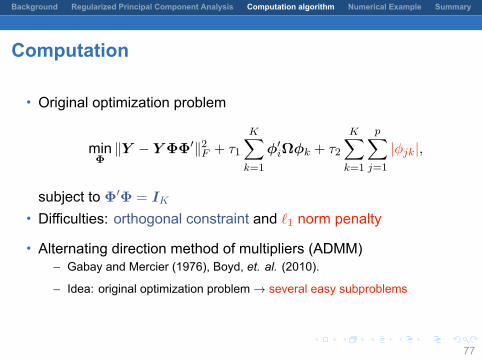
Computation
• Original optimization problem
minΦ
∥Y − Y ΦΦ′∥2F + τ1
K∑k=1
ϕ′iΩϕk + τ2
K∑k=1
p∑j=1
|ϕjk|,
subject to Φ′Φ = IK
• Difficulties: orthogonal constraint and ℓ1 norm penalty
• Alternating direction method of multipliers (ADMM)– Gabay and Mercier (1976), Boyd, et. al. (2010).
– Idea: original optimization problem → several easy subproblems
77
.
.
.
.
.
.
.
.
.
.
.
.
.
.
.
.
.
.
.
.
.
.
.
.
.
.
.
.
.
.
.
.
.
.
.
.
.
.
.
.
Background Regularized Principal Component Analysis Computation algorithm Numerical Example Summary
Computation
• Original optimization problem
minΦ
∥Y − Y ΦΦ′∥2F + τ1
K∑k=1
ϕ′iΩϕk + τ2
K∑k=1
p∑j=1
|ϕjk|,
subject to Φ′Φ = IK
• Difficulties: orthogonal constraint and ℓ1 norm penalty
• Alternating direction method of multipliers (ADMM)– Gabay and Mercier (1976), Boyd, et. al. (2010).
– Idea: original optimization problem → several easy subproblems
77

.
.
.
.
.
.
.
.
.
.
.
.
.
.
.
.
.
.
.
.
.
.
.
.
.
.
.
.
.
.
.
.
.
.
.
.
.
.
.
.
Background Regularized Principal Component Analysis Computation algorithm Numerical Example Summary
Alternating direction method of multipliers• Equivalent problem (ADMM form):
minΦ,Q,R
∥Y − Y ΦΦ′∥2F + τ1
K∑k=1
ϕ′iΩϕk + τ2
K∑k=1
p∑j=1
|rjk| ,
subject to Q′Q = IK and Φ = Q = R
• Augmented Lagrangian function:
L(Φ,Q,R,Γ1,Γ2)
=∥Y − Y ΦΦ′∥2F + τ1
K∑k=1
ϕ′iΩϕk + τ2
K∑k=1
p∑j=1
|rjk|
+ tr(Γ′2(Φ−R)) +
ρ
2∥Φ−R∥2F
+ tr(Γ′1(Φ−Q)) +
ρ
2∥Φ−Q∥2F subject to Q′Q = IK
– Γ1, Γ2:Lagrange multipliers; some ρ > 0
78

.
.
.
.
.
.
.
.
.
.
.
.
.
.
.
.
.
.
.
.
.
.
.
.
.
.
.
.
.
.
.
.
.
.
.
.
.
.
.
.
Background Regularized Principal Component Analysis Computation algorithm Numerical Example Summary
Alternating direction method of multipliers• Equivalent problem (ADMM form):
minΦ,Q,R
∥Y − Y ΦΦ′∥2F + τ1
K∑k=1
ϕ′iΩϕk + τ2
K∑k=1
p∑j=1
|rjk| ,
subject to Q′Q = IK and Φ = Q = R• Augmented Lagrangian function:
L(Φ,Q,R,Γ1,Γ2)
=∥Y − Y ΦΦ′∥2F + τ1
K∑k=1
ϕ′iΩϕk + τ2
K∑k=1
p∑j=1
|rjk|
+ tr(Γ′2(Φ−R)) +
ρ
2∥Φ−R∥2F
+ tr(Γ′1(Φ−Q)) +
ρ
2∥Φ−Q∥2F subject to Q′Q = IK
– Γ1, Γ2:Lagrange multipliers; some ρ > 078

.
.
.
.
.
.
.
.
.
.
.
.
.
.
.
.
.
.
.
.
.
.
.
.
.
.
.
.
.
.
.
.
.
.
.
.
.
.
.
.
Background Regularized Principal Component Analysis Computation algorithm Numerical Example Summary
Algorithm:at the ℓ-th iteration
Φ(ℓ+1) = argminΦ
L(Φ,Q(ℓ),R(ℓ),Γ
(ℓ)1 ,Γ
(ℓ)2
)Q(ℓ+1) = argmin
Q:Q′Q=IK
L(Φ(ℓ+1),Q,R(ℓ)Γ
(ℓ)1 ,Γ
(ℓ)2
)R(ℓ+1) = argmin
RL(Φ(ℓ+1),Q(ℓ+1),R,Γ
(ℓ)1 ,Γ
(ℓ)2
)Γ(ℓ+1)1 = Γ
(ℓ)1 + ρ
(Φ(ℓ+1) −Q(ℓ+1)
)Γ(ℓ+1)2 = Γ
(ℓ)2 + ρ
(Φ(ℓ+1) −R(ℓ+1)
)
• U (ℓ)D(ℓ)(V (ℓ)
)′= Φ(ℓ+1) +
1
ρΓ(ℓ)2 (SVD)
• Sτ (S) = sign(sik)max(|sik| − τ, 0)• All subproblems have closed-form solutions.
79

.
.
.
.
.
.
.
.
.
.
.
.
.
.
.
.
.
.
.
.
.
.
.
.
.
.
.
.
.
.
.
.
.
.
.
.
.
.
.
.
Background Regularized Principal Component Analysis Computation algorithm Numerical Example Summary
Algorithm:at the ℓ-th iteration
Φ(ℓ+1) =1
2(τ1Ω+ ρIp − Y ′Y )−1
ρ(Q(ℓ) +R(ℓ)
)− Γ1 − Γ2
Q(ℓ+1) = U (ℓ)
(V (ℓ)
)′R(ℓ+1) =
1
ρSτ2
(ρΦ(ℓ+1) + Γ
(ℓ)1
)Γ(ℓ+1)1 = Γ
(ℓ)1 + ρ
(Φ(ℓ+1) −Q(ℓ+1)
)Γ(ℓ+1)2 = Γ
(ℓ)2 + ρ
(Φ(ℓ+1) −R(ℓ+1)
)• U (ℓ)D(ℓ)
(V (ℓ)
)′= Φ(ℓ+1) +
1
ρΓ(ℓ)2 (SVD)
• Sτ (S) = sign(sik)max(|sik| − τ, 0)
• All subproblems have closed-form solutions.
80

.
.
.
.
.
.
.
.
.
.
.
.
.
.
.
.
.
.
.
.
.
.
.
.
.
.
.
.
.
.
.
.
.
.
.
.
.
.
.
.
Background Regularized Principal Component Analysis Computation algorithm Numerical Example Summary
Algorithm:at the ℓ-th iteration
Φ(ℓ+1) =1
2(τ1Ω+ ρIp − Y ′Y )−1
ρ(Q(ℓ) +R(ℓ)
)− Γ1 − Γ2
Q(ℓ+1) = U (ℓ)
(V (ℓ)
)′R(ℓ+1) =
1
ρSτ2
(ρΦ(ℓ+1) + Γ
(ℓ)1
)Γ(ℓ+1)1 = Γ
(ℓ)1 + ρ
(Φ(ℓ+1) −Q(ℓ+1)
)Γ(ℓ+1)2 = Γ
(ℓ)2 + ρ
(Φ(ℓ+1) −R(ℓ+1)
)• U (ℓ)D(ℓ)
(V (ℓ)
)′= Φ(ℓ+1) +
1
ρΓ(ℓ)2 (SVD)
• Sτ (S) = sign(sik)max(|sik| − τ, 0)• All subproblems have closed-form solutions.
80

.
.
.
.
.
.
.
.
.
.
.
.
.
.
.
.
.
.
.
.
.
.
.
.
.
.
.
.
.
.
.
.
.
.
.
.
.
.
.
.
Background Regularized Principal Component Analysis Computation algorithm Numerical Example Summary
Outline
1 Background
2 Regularized Principal Component Analysis
3 Computation algorithm
4 Numerical Example
5 Summary
81

.
.
.
.
.
.
.
.
.
.
.
.
.
.
.
.
.
.
.
.
.
.
.
.
.
.
.
.
.
.
.
.
.
.
.
.
.
.
.
.
Background Regularized Principal Component Analysis Computation algorithm Numerical Example Summary
Example: Artificial Sea Surface Temperature Data• Data settings:
Yi(sj) = ξi1φ1(sj) + ξi2φ2(sj) + ϵij ;
– j = 1, . . . , p = 2780, i = 1, . . . , n = 60– s1, . . . , s2780: located in the Indian Ocean– ξi1 ∼ N(0, 101.7), ξi2 ∼ N(0, 17.1), cov(ξi1, ξi2) = 0– ϵij ∼ N(0, 1)– (τ1, τ2): selected by 5-fold CV
φ1(s) φ2(s)
−0.04 −0.02 0.00 0.02 0.04
82

.
.
.
.
.
.
.
.
.
.
.
.
.
.
.
.
.
.
.
.
.
.
.
.
.
.
.
.
.
.
.
.
.
.
.
.
.
.
.
.
Background Regularized Principal Component Analysis Computation algorithm Numerical Example Summary
Result I: φ1(s)
True
PCA SpatPCA
−0.04 −0.02 0.00 0.02 0.04
83
.
.
.
.
.
.
.
.
.
.
.
.
.
.
.
.
.
.
.
.
.
.
.
.
.
.
.
.
.
.
.
.
.
.
.
.
.
.
.
.
Background Regularized Principal Component Analysis Computation algorithm Numerical Example Summary
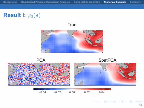
Result I: φ2(s)
True
PCA SpatPCA
−0.04 −0.02 0.00 0.02 0.04
84

.
.
.
.
.
.
.
.
.
.
.
.
.
.
.
.
.
.
.
.
.
.
.
.
.
.
.
.
.
.
.
.
.
.
.
.
.
.
.
.
Background Regularized Principal Component Analysis Computation algorithm Numerical Example Summary
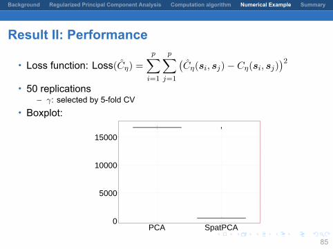
Result II: Performance
• Loss function: Loss(Cη) =
p∑i=1
p∑j=1
(Cη(si, sj)− Cη(si, sj)
)2• 50 replications
– γ: selected by 5-fold CV
• Boxplot:
0
5000
10000
15000
PCA SpatPCA
85
.
.
.
.
.
.
.
.
.
.
.
.
.
.
.
.
.
.
.
.
.
.
.
.
.
.
.
.
.
.
.
.
.
.
.
.
.
.
.
.
Background Regularized Principal Component Analysis Computation algorithm Numerical Example Summary
Result II: Performance
• Loss function: Loss(Cη) =
p∑i=1
p∑j=1
(Cη(si, sj)− Cη(si, sj)
)2• 50 replications
– γ: selected by 5-fold CV• Boxplot:
0
5000
10000
15000
PCA SpatPCA
85

.
.
.
.
.
.
.
.
.
.
.
.
.
.
.
.
.
.
.
.
.
.
.
.
.
.
.
.
.
.
.
.
.
.
.
.
.
.
.
.
Background Regularized Principal Component Analysis Computation algorithm Numerical Example Summary
Example: 8-hour average ozone data
• Region: midwestern US• Number of effective sites: 67 (irregular locations)• Number of time points: 89 days (June 3 through August 31, 1987)• At each sites, time-series is linearly detrended
−93 −83
3744
longitude
latit
ude
illinois indiana
iowa
kentucky
michigan:south
missouri
ohio
wisconsin
86

.
.
.
.
.
.
.
.
.
.
.
.
.
.
.
.
.
.
.
.
.
.
.
.
.
.
.
.
.
.
.
.
.
.
.
.
.
.
.
.
Background Regularized Principal Component Analysis Computation algorithm Numerical Example Summary
Result I: φ1(s)
PCA + interpolation SpatPCA
0.00 0.05 0.10 0.15 0.20
87

.
.
.
.
.
.
.
.
.
.
.
.
.
.
.
.
.
.
.
.
.
.
.
.
.
.
.
.
.
.
.
.
.
.
.
.
.
.
.
.
Background Regularized Principal Component Analysis Computation algorithm Numerical Example Summary
Outline
1 Background
2 Regularized Principal Component Analysis
3 Computation algorithm
4 Numerical Example
5 Summary
88

.
.
.
.
.
.
.
.
.
.
.
.
.
.
.
.
.
.
.
.
.
.
.
.
.
.
.
.
.
.
.
.
.
.
.
.
.
.
.
.
Background Regularized Principal Component Analysis Computation algorithm Numerical Example Summary
SummarySpatPCA:
• higher-dimensional analysis → (low-dimensional) structure
• with the smoothness and sparseness penalties
• enhance physical interpretation
• non-stationary spatial covariance function
• can cope with irregular locations
• simple and efficient algorithm
• R package: SpatPCA– CRAN: https://cran.r-project.org/web/packages/SpatPCA/index.html– GitHub: https://github.com/egpivo/SpatPCA
89

.
.
.
.
.
.
.
.
.
.
.
.
.
.
.
.
.
.
.
.
.
.
.
.
.
.
.
.
.
.
.
.
.
.
.
.
.
.
.
.
Background Regularized Principal Component Analysis Computation algorithm Numerical Example Summary
Thanks for your attention!
90