regular self-oscillating and chaotic dynamics of a continuous stirred tank reactor

Computers and Chemical Engineering 26 (2002) 889–901

Regular self-oscillating and chaotic dynamics of a continuousstirred tank reactor

Manuel Perez a,*, Rafael Font b, Marco A. Montava a,1

a Departamento de Fısica Ingenierıa de Sistemas y Teorıa de la Senal, Uni�ersidad de Alicante, Escuela Politecnica Superior,Campus de San Vicente, 03071 Alicante, Spain

b Departamento de Ingenierıa Quımica, Uni�ersidad de Alicante, Campus de San Vicente, Apartado 99, Alicante, Spain

Received 4 June 2001; received in revised form 29 January 2002; accepted 29 January 2002

Abstract

A continuous stirred tank reactor for propylene glycol production is shown in this paper, analyzing the regular, self-oscillatingand chaotic dynamics, which can appear under specific operating conditions. The paper shows that there is a small interval ofconcentration and temperature of the inlet stream to the reactor, that produces self-oscillating behavior, taking into account thevariation of eigenvalues of the linearized system at the equilibrium point, both the multi-dimensional and two-dimensionalsimplified models of the reactor. The conditions that produce chaotic dynamics are researched when the reactor is inself-oscillating regime, showing that a coolant flow rate periodic variation can produce chaotic behavior. Through thedetermination of chaotic maps, bifurcation diagrams, the existence of a new set of strange attractors has been tested, showing thatthe mechanism of chaos is due to the transition from quasi-periodic initial state. A short explanation of the simulation programsis also presented. © 2002 Elsevier Science Ltd. All rights reserved.

Keywords: Reactor; Dynamics; Regular; Self-oscillating; Chaotic; Simulation

Nomenclature

heat transfer area (m2)Aj

V�/Q0 dimensionless parameterc0

c0C �A0/C �B0 dimensionless parameterc01

c0C�A0/C �C0 dimensionless parameterc02

V��HRRC �A0/FA0CpsE dimensionless parameterc1

c2 UAj/FA0Cps dimensionless parameterVQj/Q0Vj dimensionless parameterc3

VUAj/Q0/�jcpj dimensionless parameterc4

CA concentration of propylene oxide (kmol/m3)C �A0 steady state concentration of propylene oxide after the startup (kmol/m3)

inlet concentration of propylene oxide (kmol/m3)CA0

CB concentration of water+sulfuric acid (kmol/m3)steady state concentration water+sulfuric acid after startup (kmol/m3)C �B0

inlet concentration of water+sulfuric acid (kmol/m3)CB0

concentration of propylene glycol (kmol/m3)CC

www.elsevier.com/locate/compchemeng

* Corresponding author. Tel.: +34-96-5903482; fax: +34-96-5903682.E-mail addresses: [email protected] (M. Perez), [email protected] (R. Font), [email protected] (M.A. Montava).1 Fax: +34-96-5903826.

0098-1354/02/$ - see front matter © 2002 Elsevier Science Ltd. All rights reserved.PII: S0098-1354(02)00015-7

mailto:[email protected]



M. Perez et al. / Computers and Chemical Engineering 26 (2002) 889–901890

C �C0 steady state concentration of propylene glycol after the startup (kmol/m3)concentration of methanol (kmol/m3)CM

CM0 inlet concentration of methanol (kmol/m3)heat capacity of propylene oxide (kJ/kg K)cpA

heat capacity of water+sulfuric acid (kJ/kg K)cpB

heat capacity of propylene glycol (kJ/kg K)cpC

cpj heat capacity of coolant flow rate (kJ/kg K)heat capacity of methanol (kJ/kg K)cpM

Q0cpm/FA0cpscy

activation energy (kJ/kmol)Evolumetric flow rate of cooling water (m3/s)Fj

Q0 volumetric flow rate for the inlet stream (m3/s)volumetric flow rate for the outlet stream in steady state (m3/s)Qj

FA0 molar flow rate of propylene oxide for the inlet stream (kmol A/s)molar flow rate of water+sulfuric acid for the inlet stream (kmol B/s)FB0

FM0 molar flow rate of methanol for the inlet stream (kmol M/s)�e−E/RTk

R perfect-gas constant (kJ/kmol K)Q0t/V dimensionless timet*reactor temperature (°C)Tset point temperature (°C)Tset

T0 inlet stream temperature for the startup (°C)jacket temperature (°C)Tj

inlet stream cooling water temperature for the startup (°C)Tj0

overall heat transfer in the jacket (kJ/s m2 °C)Ureactor volume (m3)Vjacket volume (m3)Vj

�*t* dimensionless variablex6

xa CA/C�A0 dimensionless concentration of ACA0/C�A0 initial dimensionless concentration of Axa0

xb CB/C�B0 dimensionless concentration of BCB0/C�B0 initial dimensionless concentration of Bxb0

xc CC/C�C0 dimensionless concentration of CCM/C�M0 dimensionless concentration of Mxm

RT/E dimensionless temperature of the reactoryRT0/E dimensionless temperature for the inlet stream to the reactory0

RTj/E dimensionless temperature in the jacketzzj0 RTj0/E dimensionless temperature for the inlet coolant flow

Greek symbols�j time constant for the dynamic of the jacket�R time constant for the reactor� coolant flow rate perturbation frequency (rad/s)

�(V/Q0) dimensionless perturbation frequency�*density of the coolant water (kg/m3)�j

molar density of propylene oxide for the inlet stream (kmol A/m3)�A0

molar density of water+sulfuric acid for the inlet stream (kmol B/m3)�B0

molar density of methanol for the inlet stream (kmol M/m3)�M0

enthalpy of reaction (kJ/kmol)�HR

1. Introduction

The study of a continuous stirred tank reactor(CSTR) in which a simple irreversible reaction A�Boccurs, has been considered in the past (Aris &

Amundson, 1958; Aris, 1969; Kevrekidis, Aris, &Schmidt, 1986; Kubickova, Kubicek, & Marek, 1987),showing evidence of limit cycles and self-oscillatingbehavior, and demonstrating the complexity anddiversity of the structures exiting in a CSTR and also in

M. Perez et al. / Computers and Chemical Engineering 26 (2002) 889–901 891

a semi-batch reactor. The bifurcation analysis for asemi-batch and a CSTR reactor (Planeaux & Jensen,1986; Teymour & Ray, 1989; Teymour, 1997), revealeda higher degree of complexity, observing the possibilityof regular to chaotic behavior. Since the Hopf classicalwork (Marsden & McCraken, 1976), applied to afirst-order irreversible reaction by Uppal, Ray, andPoore (1974), numerous examples of the Hopfbifurcation phenomena linked to self-oscillation havebeen described for some chemically reacting systems(Vaganov, Samoilenko, & Abranov, 1978; Zhabotinsky& Rovinskii, 1984). In the paper of Mankin andHudson (1984), it has been shown that a CSTR can bedriven to chaos by perturbing the cooling temperature,deducing by means of numerical simulation thatperiodic, quasi-periodic and chaotic behaviors canappear depending on the values of the amplitude andfrequency of the periodic imposed disturbance.Experimental evidence that an oscillatory system canproduce chaos also appears in the periodically forcednonlinear oscillators in non-chemical systems (Tomita,1986). It must nevertheless be emphasized that anexternal forcing CSTR is a very appropriate system inthe study of transition from regular and self-oscillatingto chaotic behavior, taking into account the rigidnon-linear dependence of the kinetic constants withtemperature.

In this paper, regular self-oscillating and chaoticdynamics of an exothermic CSTR for propylene glycolproduction is considered. Regular behavior means thereactor reaches a steady state with constanttemperature and concentrations values. Thethermodynamic data for the reaction has been takenfrom Fogler (1999). This model is defined by fivenon-linear differential equations and one lineardifferential equation, where the reaction is first-orderwith respect to the propylene glycol. From the previouspapers cited, the analysis of an external forced CSTR iscarried out considering only two independent variablesi.e. concentration and temperature in the reactor, so thestudy of a forced CSTR is restricted to atwo-dimensional system. However, in this paper, amore exact multi-dimensional model is considered as astarting point, taking into account the dynamic of thejacket of the reactor and the presence of inertcomponents in the reaction. Nevertheless, due to thefact that in terms of dimensionality, a second-ordersimplified system is complicated enough to exhibit thephenomena of quasi-periodicity, self-oscillation andchaos, the simplified two-dimensional model is deducedfrom the multi-dimensional model, where the extradimension obtained from the periodic volumetric flowrate cooling, is responsible for the dynamiccomplications.

The paper shows that there are intervals of the inletflow temperature and concentration, which produce a

small region or lobe where the reactor has aself-oscillating basic state without any periodic externaldisturbance. Then, a periodic variation of the coolantflow rate to the reactor jacket, depending on the valuesof the amplitude and frequency can drive the reactor toa limit cycle and throughout a non-steady state tochaos, considering both the multi-dimensional and thetwo-dimensional model. The maps of amplitude vs.frequency of cooling water disturbance are obtainedwhen the values of inlet flow temperature andconcentration are inside the lobe from which thebifurcation diagrams can be determined, showing thatthe mechanism of chaos is due to the transition from aquasi-periodic state.

2. CSTR model equations

The exothermic reaction for propylene glycol produc-tion (C) from propylene oxide (A) and water containinga small quantity of H2SO4 (B) and methanol (M) isconsidered in a CSTR.

The reaction is carried out with a water excess, sofirst-order in reactant A and zero- order with respect toM can be considered. The reactor has an external jacketto eliminate the heat during the reaction.

A continuos stream of cooling water flows along thejacket, and it has been assumed that there is a goodmixing of the water inside the jacket, and consequentlya mean temperature, that can vary with time, is consid-ered in the jacket.

The components A, B, C, M mass balance aredefined by the following equations;

dCA

dt=

Q0

V(CA0−CA)−kCA (1)

dCB

dt=

Q0

V(CB0−CB)−kCA (2)

dCC

dt=

Q0

V(−CC)+kCA (3)

dCM

dt=

Q0

V(CM0−CM) (4)

k=�e−E/RT (5)

Taking into account that the water is in excess, thereaction velocity of Eqs. (1)– (3) is approximated by−rA= −rB=rC�kCA. The Eq. (5) is the Arrheniuslaw, CA0, CB0, CC0 and CM0 are the molar concentra-tions for the inlet stream, T is the reactor temperature,CA, CB, CC and CM are the molar concentrations for


the outlet stream, Q0 is the volumetric flow rate forthe inlet stream, and V is the volume of the reactor.From the molar flow rates of A, B and M, the inletvolumetric flow rate Q0 is determined by the equa-tion:

Q0=FA0

�A0

+FB0

�B0

+FM0

�M0

(6)

where FA0, FB0, FM0 are the molar flow rates for theinlet stream and �A0, �B0, �M0 the molar densities ofpure components A, B, M. The values of inlet con-centrations CA0, CB0 and CM0 are determined by theequations

CA0=FA0

Q0

; CB0=FB0

Q0

; CM0=FM0

Q0

(7)

The energy balance for the reactor can be writtenas

VcPR

dTdt

=FA0cPS(T0−T)+ (−�HR)�CAVe−E/RT

− UAj(T−Tj) (8)

where −�HR is the enthalpy of reaction, U is theoverall heat transfer coefficient of the jacket, Aj is theheat transfer area, Tj is the jacket temperature and T0

the inlet stream temperature. The parameter cPS isdefined by the equation:

cPS=cPA+FB0

FA0

cPB+FM0

FA0

cPM (9)

where cPA, cPB, cPM are the molar heat capacities forA, B, M respectively. The value of cPR is calculatedby the equation:cPR=cPACA+cPBCB+cPCCC+cPMCM (10)

where cPC, CC are the molar heat capacities and theconcentration for the propylene glycol.

The energy balance for the jacket is

dTj

dt=

Qj

Vj

(Tj0−Tj)+UAj

�jcPjVj

(T−Tj) (11)

where Qj, �j, cpj are the volumetric flow rate, thedensity and the heat capacity of cooling water respec-tively, Vj is the volume of the jacket and Tj0, Tj arethe inlet cooling flow rate temperature and the meanvalue temperature of the jacket respectively. Takinginto account the dimensionless variables defined byTable 1, the CSTR equations are the following

dxa

dt*=xa0−xa−c0xae−1/y

dxb

dt*=xb0−xb−c01xae−1/y

dxc

dt*= −xc−c02xae−1/y

dxm

dt*=xmo−xm

cy

dydt*

=y0−y−c1xae−1/y−c2(y−z)

dzdt*

=c3(zj0−z)+c4(y−z)

��

(12)

where the parameter cy depending on the absolutevariables CA, CB, CC, CM or dimensionless variablesxa, xb, xc, xm is given by the equation

cy=Q0

FA0cPS

(cPAC �A0xa+cPBC �B0xb+cPCC �C0xc

+cPMC �m0xm) (13)

From Eq. (12), it can be deduced that the variablexm is independent of the others variables, however itis necessary to calculate the variable parameter cy

given by Eq. (13). Table 2 shows the parameter val-ues of the reactor and nominal operating conditions.

The model represented by Eq. (12) can be sim-plified taking into account that the value cy is ap-proximately constant (around to one), so Eq. (12)became

dxa


dydt*

=1cy

[y0−y−c1xae−1/y−c2(y−z)]

dzdt*

=c3(zj0−z)+c4(y−z)

��

(14)

Table 1Dimensionless variables

Definition DefinitionDimensionless Dimensionlessvariable variable

Q0t/V x6t* �*t*V�/Q0c0xa CA/C �A0

c01 c0C �A0/C �B0CA0/C �A0xa0

c02 c0C �A0/C �C0CB/C �B0xb

CB0/C �B0xb0 cy Q0cpm/FA0cps

CC/C �C0xc c1* V��HRRC �A0

FA0cpsEc2*xm CM/C �M0

c1xm0 c1*/c2*CM0/C�M0

c2y UAj/FA0cpsRT/EVQj/Q0Vjc3y0 RT0/E

RTj/Ez c4* VUAj/Q0

RTj0/E c4*/�jcpjc4zj0

Superscript (�) denotes steady-state values after the startup.


Table 2Nominal operating conditions and parameter values

ValueDescriptionVariable

Molar flow rate of propylene oxide forFA0 7.55×10−3

the inlet stream (kmol A/s)Molar flow rate of water+sulfuric acid 1.28×10−1FB0

for the inlet stream (kmol B/s)Molar flow rate of methanol for theFM0 1.26×10−2

inlet stream (kmol M/s)Volumetric flow rate for the inlet streamQ0 3.33×10−3

(m3/s)�A0 Molar density of propylene oxide for 14.78

the inlet stream (kmol A/m3)Molar density of water+sulfuric acid 55.27�B0

for the inlet stream (kmol B/m3)Molar density of methanol for the inlet�M0 24.67stream (kmol M/m3)

14.16Reactor volume (m3)VJacket volume (m3)Vj 1.416Pre-exponential factor from Arrhenius 4.71×109�

law (s−1)E 75 414Activation energy (kJ/kmol)

Overall heat transfer in the jacketU 5.590kJ/(s m2 °C)Heat transfer area (m2)Aj 33Heat capacity of propylene oxide 146.52cpA

(kJ/kg K)Heat capacity of water+sulfuric acidcpB 75.35(kJ/kg K)

cpC Heat capacity of propylene glycol 192.57(kJ/kg K)

cpM 81.63Heat capacity of methanol (kJ/kg K)Heat capacity of coolant flow rate 4.18cpj

(kJ/kg K)Qj 2Q0Standard coolant flow rate (m3/s)�j Density of the coolant water (kg/m3) 1000

Inlet stream temperature for the startupT0 15.2(°C)Inlet stream cooling water temperatureTj0 15for the startup (°C)

R Perfect-gas constant (kJ/kmol K) 8.314�HR Enthalpy of reaction (kJ/kmol) −83 793

Inlet concentration of propylene oxide 2.26CA0

(kmol/m3)Inlet concentration of water+sulfuricCB0 38.4acid (kmol/m3)

CM0 Inlet concentration of methanol 3.76(kmol/m3)

If �R��j the jacket’s dynamic can be considerednegligible. This means that the jacket’s temperature isvery close to that of the reactor, and the variable z(dimensionless temperature in the jacket) can be elim-inated from Eq. (14) as follows:

z=c3zj0+c4y

c3+c4

(16)

Substituting z in Eq. (14) the following equationsare obtaineddxa


dydt*

=1cy

[y0−y+c1xae−1/y−c5(y−zj0)] (17)

where c5= (c2c3)/(c3+c4). Eq. (17) are a two-dimen-sional model of the reactor, which can been used forcorroborating the existence of self-oscillating andchaotic behavior. In this paper, a multi-dimensionalmodel given by Eq. (12) and the two-dimensional ap-proximate one defined by Eq. (17) is considered.

3. Analysis of regular and self-oscillating region

In order to study the regular and self-oscillatingbehavior, the reactor is started up from an initialcondition where there is 55.3 kmol/m3 of a mixture ofwater with a small quantity of sulfuric acid, and 4.8kmol/m3 of methanol. The initial reactor and fluidjacket temperature are T=24 °C and Tj=23.7 °Crespectively. The flow rate feed stream consists ofFA0=36.3 kmol/h, FB0=462.7 kmol/h and FM0=45.4kmol/h. With these values, taking the left-hand sideof Eqs. (1)– (4) and (8) and Eq. (11) equal to zero, orsimulating these equations, the following steady statevalues are obtained: C �A0=0.95 kmol/m3, C�B0=37kmol/m3, C�C0=1.3 kmol/m3, C�M0=3.7 kmol/m3.These values are used as a reference to introduce thedimensionless concentrations shown in Table 1.

The following step in the study of self-oscillatingand regular behavior is the equilibrium points analy-sis. The Eq. (12) can be written in a compact form asfollows;

x� (t)= f [x(t)] (18)

then, a point x*� [xa*, xb*, x c*, xm*, y*, z*] is said tobe an equilibrium point of the vector field f(.) iff(x*)=0. At the critical point x*, the variation ofvariables x vanishes so that the system cannot moveout this point. However, Eq. (18) says nothing aboutwhether the point x* is stable or unstable againstperturbations. From Eq. (12) it is easy to deduce theequilibrium equations:

On the other hand, Eq. (14) can be simplified con-sidering the dimensionless time constant for the reac-tor, �R, and the dynamics of the jacket, �j; whosevalues are

�R=�1+c2

cy

�−1

; �j= (c3+c4)−1 (15)


xa0−xa*−c0xa*e−1/y*=01cy*

[y0−y*+c1xa*e−1/y*−c2(y*−z*)]=0

c3(zj0−z*)+c4(y*−z*)=0

��

(19)

Note that Eq. (19) are valid for the multi-dimen-sional model defined by Eq. (12), and for the sim-plified models defined by Eq. (14) and Eq. (17)respectively. From Eq. (19) it is possible to obtain theflow inlet dimensionless temperature y0 as a functionof the equilibrium temperature in the reactor y*, as-suming that the flow inlet dimensionless concentrationxa0 is a known value

y0= (1+c5)y*−c5zj0−c1xa0

e1/y*+c0

(20)

Eq. (20) is plotted in Fig. 1 for different values ofxa0.

The number of the equilibrium states depends onthe number of points where the straight line y0=con-stant intersects with the curve y0= f(y*). From Fig.1, it is deduced that for xa0=20, and a constantvalue of y0�0.015, there are three equilibrium pointsP1, P2, P3, being P1 stable, P2 unstable and P3 can bestable or unstable, depending on the eigenvalues ofthe linearized system at this point (Fogler, 1999).

A bifurcation point appears when y0=constant istangent to y0= f(y*) at a maximum or minimumpoint. So, considering dy0/dy*=0 in Eq. (20) andtaking into account Eq. (19), the following equationsare deduced:

xa0=1+c5

c1

(y*)2e−1/y*(e−1/y*+c0)2

y0= (1+c5)y*−c5zj0− (1+c5)(y*)2(1+c0e−1/y*)(21)

These equations represent the bifurcation curve asa function of parameter y* (equilibrium temperatureof the reactor). This curve with a cusp point, is theborder that divides the plane xa0–y0 at one and threeequilibrium states respectively.

The nature of the one equilibrium point is deducedfrom the eigenvalues of the Jacobian matrix of theEq. (12), so the following equation is obtained;

Fig. 1. Inlet dimensionless temperature y0 vs. equilibrium point y* atdifferent values of xa0.

Eq. (22) can be written as

��I−J �= (�+1)3(�3+S1�2+S2�+S3)=0 (23)

where (−1) jSj is the sum of the jth principal minorsof determinant �; S1= − trace of matrix �, S3= −determinant of �.

From Eq. (23), it is deduced that the reactor willbe in self-oscillation regime if this equation has twocomplex roots with the real part equal to zero. Tak-ing into account the Routh–Hurwitz stability crite-rion (Stephanopoulos, 1991), it is deduced that theconditions

S1�0; S2�0; S3�0; S1S2−S3=0 (24)

imply self-oscillating behavior, and the roots ofequation

S1�2+S3=0 (25)

give us the frequency of self-oscillations. Conse-quently, from Eq. (24) and Eq. (25), it is possible toobtain the values of xa0, y0 as a function of y*, fromwhich the reactor has an oscillating behavior withoutany periodic external disturbance force.

For the reactor two-dimensional model given byEq. (17), the Eq. (20) are valid, and the self-oscillat-ing condition is obtained by equation

��I−J �= (�+1)3

��

�+1+c0e−1/y* c0

xa*(y*)2e

−1/y* 0

−c1

cy*e−1/y*

�−1cy*�

− (1+c2)+c1

xa*(y*)2e

−1/y*n −c2

cy*0 −c4 �+c3+c4

��

= (�+1)3� (22)


Fig. 2. Self-oscillating and three-equilibrium state regions for themulti-dimensional and two-dimensional model.

and in this case it is very difficult to obtain similarequations to Eq. (27), thus necessitating a computa-tional solution. Eqs. (21) and (24) and Eq. (27) areplotted in Fig. 2. This Figure shows that when thevalues of xa0 and y0 are inside the lobe, the reactor hasa self-oscillating behavior, both the multi-dimensionalmodel and the two-dimensional one (Appendix A(1)).

Note that a coordinates point xa0, y0 inside the lobecorresponds to an equilibrium point xa*, y*, z* given bythe equations

xa0=xa*(1+c0e−1/y*)

y0= (1+c5)y*−c5zj0−c1xa

0

c0+e1/y

z*=c3zj0+c4y*

c3+c4

��

(28)

In this case, the Jacobian system (both multi-dimen-sional model and two-dimensional model) has someeigenvalues with real part positive and so this equi-librium point will be unstable, and the correspondingsystem trajectory approaches to a limit cycle.

For a point (xa0, y0) outside the lobe, there is onlyone equilibrium point, this means that the values ofinlet composition concentration xa0 of component A,and the inlet stream temperature y0, give a curve suchas the straight line y0=constant intersects to the bifur-cation curve of Fig. 1 only at one point P.

Other interesting aspect is that the lobe is very small,and so it is very difficult to choose values of tempera-ture and propylene oxide concentration in the inletstream of the reactor, to produce an oscillating regime,and consequently the chaotic behavior remains hidden,as will be shown later.

Fig. 3 shows the frequency that corresponds exactlyto the lobe curve points, and so it is possible to deducean approximate value of the period of self-oscillationfor a values (xa0, y0) given inside the lobe, by interpola-tion. Note that for high input concentrations and lowinput temperatures, the frequency tends to a constantvalue of approximately 4 rad/unit of dimensionlesstime.

Figs. 4 and 5 show a stationary and self-oscillatingbehavior with the multi-dimensional model consideringvalues xa0, y0 out and inside the lobe respectively. Fig.5 shows that a trajectory approaches a closed curve orlimit cycle and remains there. The spiral in the core partof Fig. 5 represents the transient state, and the final

Fig. 3. Self-oscillating frequency vs. inlet dimensionless temperaturefor the multi-dimensional and two-dimensional model.

From the two complex roots with real part equal tozero condition (�=0), the equations of self-oscillatingbehavior are deduced

xa0=c0(y*)2

c1

�3+c6+

�2+c5

c0

�e−1/y*+c0e−1/y*n

y0= (1+c5)y*−c5zj0− (y*)2[2+c5+c0e−1/y*] (27)

where the values of xa0 and y0 are obtained from theequilibrium Eq. (19), substituting x*a in Eq. (26) andoperating, from the condition �=0, Eq. (27) arededuced.

Note that the self-oscillating condition for the multi-dimensional model is given by Eq. (24) and Eq. (25),

��I−J �=

��

�+1+c0e−1/y* c0

xa*(y*)2 e−1/y*

−c1

cy*e−1/y*

�−1cy*�

− (1+c2)+c1

xa*(y*)2 e−1/y*n

��

=0 �2−��+�=0 (26)


steady state is the closed curve. Similar plots can beobtained for the two-dimensional model.

4. Chaotic behavior

The theory of oscillations is a well developed field, andthe qualitative features of the main models of oscillationhave been previously applied to systematic experimentaland theoretic studies of chemical oscillations, both innumerical and experimental studies (Guckenheimer &Holmes, 1983; Planeaux & Jensen, 1986). However, in thefield of the reactor oscillations, a dynamic object isactually very important, i.e. the strange attractor whichappears when the reactor has chaotic behavior. In orderto carry out theoretical and experimental studies of thisdynamic object, the following steps are necessary:

1. The development of a mathematical model based onplausible chemical schemes.

2. The analysis and design of chemical reactors basedon simple reactions.

3. The possibility of simulating the mathematicalmodel with a clear criteria to elucidate betweenchaos and transient chaos.

With these ideas in mind, the study of chaotic behav-ior in a reactor is carried out taking into account themulti-dimensional model and the simplified one givenby Eq. (12) and Eq. (17) respectively.

The chaotic behavior is researched assuming that thevalues of xa0 and y0 are inside of the lobe of Fig. 2, andthat the coolant flow rate is varied according to theequation:

Qj=Q� j+Qmj sin(�t) 0�Qmj�Q� j (29)

It is important to point out that this external forcingdisturbance, which can produce chaotic behavior, isvery easy to implement through a control valve.

Taking into account Table 1, Eq. (29) in dimension-less form are written as

c3= c3+cm3 sin(�*t*)= c3+cm3 sin(x6)

0�cm3� c3 (30)

where the x6 dimensionless variable is introduced toeliminate the time between Eq. (11) and Eq. (29) con-sidering a new dimensionless equation defined by

dx6

dt*=�* ; 0�x6�2� (31)

so Eq. (12) and Eq. (31) are an autonomous dynamicalsystem independent of time.

With cm3=0 or �*=0 the reactor is not forced anddue to the fact that xa0, y0 are inside the lobe, thereactor reaches a limit cycle. The effect of a disturbancein the coolant flow rate can drive the reactor to anon-periodic oscillatory state. In order to investigatethis possibility, the chaotic regions maps for the two-di-mensional and multi-dimensional models are obtainedby simulating the system with two very close initialconditions for a long period (Appendix A(3)). The ideais to eliminate resonances and phase-locking phenom-ena, i.e. the so-called soft chaos (Lichtenberg & Lieber-man, 1992). With the values xa0=5 and y0=0.0285 i.e.points inside the lobe (Fig. 2), the two-dimensionalmodel and the multi-dimensional one, have been simu-lated with different combinations of the dimensionlessamplitude cm3 and dimensionless frequency �*. Fig. 6shows the results obtained. Points of Fig. 6 show thepresence of chaotic islands and regions without points,where the reactor reaches an oscillatory steady state.This chaotic islands are fractals.

With this map, it is possible to obtain the bifurcationdiagrams. Taking a fixed value of the dimensionless

Fig. 4. Regular behavior for the multi-dimensional model with valuesxa0=6, y0=0.029 outside the lobe. Initial conditions x(0)= [1 1 10.033 0.0329].

Fig. 5. Self-oscillating behavior for the multi-dimensional model withvalues xa0=5, y0=0.0285 inside the lobe. Initial conditions at theequilibrium point x(0)= [1.36 0.94 2.64 0.0337 0.0335 0].


Fig. 6. Chaotic maps (a) two-dimensional model, (b) multi-dimen-sional model.

small intervals of �* in which the evolution of thereactor abruptly becomes periodic again. For examplein Fig. 7a, with �*�2.01 the system is chaotic, butwith �*�2.02 the system is periodic with period-3.

The bifurcation diagram is an important tool forinvestigating interesting oscillating regimes of the reac-tor. While initially our discussion was focused uponvariation of �* with cm3 constant, it is possible toconsider the reverse order situation, i.e. with �* con-stant and cm3 variable. In this case new chaotic regimesand strange attractors appear, both with the two-di-mensional and the multi-dimensional model of the reac-tor. The bifurcation diagram shows another interestingfact, i.e. the chaos mechanism is generated by a transi-tion from a quasi-periodic initial state. The speed of theappearance of the chaos depends on the values of cm3,�*, for example considering Fig. 7a, and beginningwith �*=1.7, the entire transition from the quasi-peri-odic initial state takes place for 1.73��*�1.75, andfor values �*�1.75 the chaotic behavior is reached.This mechanism is not evident without the bifurcationdiagram, because the two-dimensional model has threeequilibrium points at the phase plane, one of them is asaddle point, and the remainder are stable. On theother hand, it is well known that the perturbation ofstable and unstable manifolds which cross at the saddlepoint can produce chaos (Wiggins, 1990; Guckenheimer& Holmes, 1983; Seydel, 1994; Lichtenberg & Lieber-man, 1992). Consequently, it could be deduced that theperturbation in the coolant flow rate is the responsiblefor the formation of the so-called homoclinic tangle. Itis clear that this conclusion is wrong. Fig. 8 shows thetrajectories at the phase plane without any homoclinicor heteroclinic orbit, and the situation of the strangeattractor for a values of cm3, �*. From this Figure, itcan be deduced that the separatrix line does not inter-sect with the stable manifolds lines p2p1 and p2p3 and

Fig. 7. Bifurcation diagram obtained with xa0=5, y0=0.0285. (a)Two-dimensional model with cm3=9, (b) multi-dimensional modelwith cm3=9.

Fig. 8. Phase plane with equilibrium points and strange attractor forthe two-dimensional model.

amplitude of the coolant flow rate cm3=9 (Fig. 6), andmodifying the dimensionless angular frequency �*from 1.7 to 2.15 as shown in Fig. 6a and from 1.8 to 2.6as shown in Fig. 6b, the bifurcation diagrams areobtained in Fig. 7 for the two-dimensional model andthe multi-dimensional model respectively (AppendixA(4)).

In Fig. 7, the dimensionless temperature is plotted vs.the forcing dimensionless frequency �*. The tempera-ture at the beginning of each forcing cycle shows inter-vals of periodic behavior, where the reactor has a singlevalue of temperature (1.7��*�1.75), then a chaoticregion where the reactor has an unpredictable tempera-ture (1.7��*�1.87), four different values (four cyclesfrom 1.87��*�1.88), a small chaotic region and soon. The result is a very complex window pattern, wherewe can see that, within the chaotic regions, there are


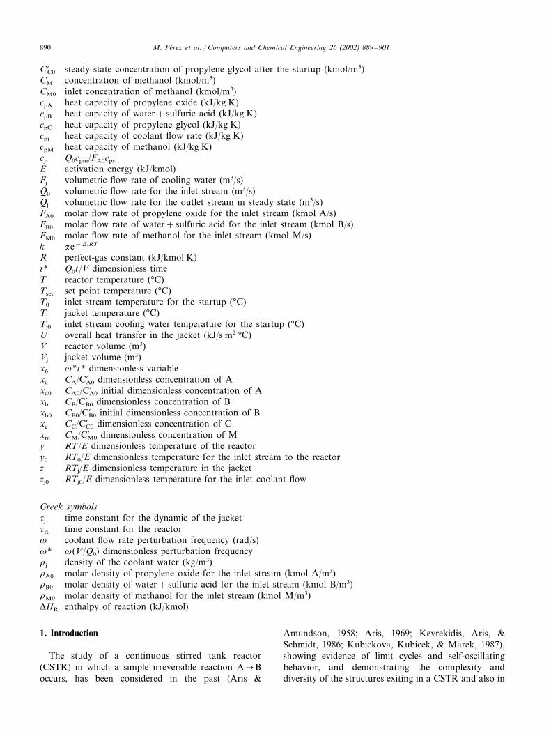
Fig. 9. Sensitive dependence for the exact model of the reactor withxa0=5, y0=0.0285 obtained from Fig. 6b with cm3=9 and �*=1.9.

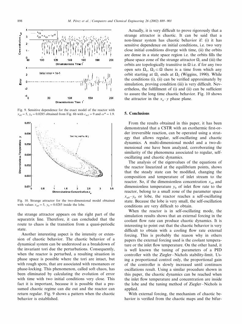
Actually, it is very difficult to prove rigorously that astrange attractor is chaotic. It can be said that anon-linear system has chaotic behavior if: (i) it hassensitive dependence on initial conditions, i.e. two veryclose initial conditions diverge with time, (ii) the orbitsare dense in a state space region i.e. the orbits fills thephase space zone of the strange attractor �, and (iii) theorbits are topologically transitive in � i.e. if for any twoopen sets �1, �2�� there is a time from which anyorbit starting at �1 ends at �2 (Wiggins, 1990). Whilethe conditions (i), (ii) can be verified approximately bysimulation, proving condition (iii) is very difficult. Nev-ertheless, the fulfillment of (i) and (ii) can be sufficientto assure the long time chaotic behavior. Fig. 10 showsthe attractor in the xa–y phase plane.

5. Conclusions

From the results obtained in this paper, it has beendemonstrated that a CSTR with an exothermic first-or-der irreversible reaction, can be operated using a strat-egy that allows regular, self-oscillating and chaoticdynamics. A multi-dimensional model and a two-di-mensional one have been analyzed, corroborating thesimilarity of the phenomena associated to regular, self-oscillating and chaotic dynamics.

The analysis of the eigenvalues of the equations ofthe reactor linearized at the equilibrium points, showsthat the steady state can be modified, changing thecomposition and temperature of inlet stream to thereactor. So, if the dimensionless concentration xa0 anddimensionless temperature y0 of inlet flow rate to thereactor, belong to a small zone of the parameter spacexa0–y0 or lobe, the reactor reaches a self-oscillatingstate. Because the lobe is very small, the self-oscillationconditions are very difficult to obtain.

When the reactor is in self-oscillating mode, thesimulation results shows that an external forcing in thecoolant flow rate can produce chaotic dynamics. It isinteresting to point out that the chaotic behavior is verydifficult to obtain with a cooling flow rate externalforcing. This is probably the reason why in otherspapers the external forcing used is the coolant tempera-ture or the inlet flow temperature. On the other hand, itis well known the tuning of parameters of a PIDcontroller with the Ziegler–Nichols stability-limit. Us-ing a proportional control only, the proportional gainof the controller is slowly increased until continuososcillations result. Using a similar procedure shown inthis paper, the chaotic dynamics can be reached whenthe inlet flow temperature and concentration are insidethe lobe and the tuning method of Ziegler–Nichols isapplied.

With external forcing, the mechanism of chaotic be-havior is verified from the chaotic maps and the bifur-

Fig. 10. Strange attractor for the two-dimensional model obtainedwith values xa0=5, y0=0.0285 inside the lobe.

the strange attractor appears on the right part of theseparatrix line. Therefore, it can concluded that theroute to chaos is the transition from a quasi-periodicstate.

Another interesting aspect is the intensity or exten-sion of chaotic behavior. The chaotic behavior of adynamical system can be understood as a breakdown ofthe invariant tori due the perturbations. Consequently,when the reactor is perturbed, a resulting situation inphase space is possible where the tori are intact, butwith rough spots, that are associated with resonances orphase-locking. This phenomenon, called soft chaos, hasbeen eliminated by calculating the evolution of errorwith time with two initial conditions very close. Thisfact it is important, because it is possible that a pre-sumed chaotic regime can die out and the reactor canreturn regular. Fig. 9 shows a pattern when the chaoticbehavior is established.


cation diagram. Consequently, the route to chaos isidentified as a transition from a quasi-periodic state,which is reached when an external forcing in thecoolant flow rate is applied. In this case, the presence ofa new set of strange attractors was verified viasimulation.

The phenomena considered previously should betaken into consideration by the control engineer. ACSTR with PI control can be investigated following thesame procedure shown in this paper, in order to obtainself-oscillating and chaotic behavior taking into ac-count the control valve saturation. More elaboratemodels of chemical reactors, with complex kinetics canbeen used to plan experimental studies with PI con-trollers and with more sophisticated control systems.

Appendix A. Development of computational algorithms

In this appendix the principal steps of the algorithmsused throughout the paper are briefly discussed. All theprograms have been designed by using a C+ + com-piler and the Matlab compiler, which takes .m-files asinput and generates C+ + source code as output.

A.1. Determination of the lobe and the cur�e with cusppoint

Eq. (20) are valid for the two-dimensional model andthe exact model. Eq. (23) and Eq. (26) represent theself-oscillating zone for the exact and two-dimensionalmodels respectively. From Fig. 1, one takes a minimumvalue (yamin) and maximum value (yamax) of y*around the maximum at Fig. 1. It can be proved thatthe lobe and cusp point appear approximately betweenyamin and yamax. Then Eq. (21) and Eq. (27) arecalculated for the y* values range: yamin�y*�ya-max. For the multi-dimensional model, there are noequations for the lobe and it is necessary to develop thedeterminant principal minors of D:

The objective is to determine pairs of equilibrium val-ues (xa*, y*) that test Eq. (24), and with these valuesfrom the equilibrium Eq. (19), the following relation-ships are obtained:

xa0= f1(y*,xa*)y0= f2(y*,xa*)

�(A2)

Eq. (A2) represent the dimensionless composition andtemperature of propylene oxide in the inlet flow rate tothe reactor, which produces self-oscillating behavior.Note that from xa*, y* and Eq. (12), the equilibriumvalues xb*, x c*, z* are deduced. The value xm* is indepen-dent of xa*, y*. The calculations are carried out throughthe following stages:(i) From determinant (A1), S1, S2,S3 are calculated as

S1=�1+c0e−1/y*+ (c3+c4)cy*+ (1+c2−c1)

e−1/y*

(y*)2 xa*�

cy*=

S �1cy*

(A3)

S2=1cy*�

(1+c3+c4+c0e−1/y*)(1+c2)− (1+c3+c4)

c1

e−1/y*

(y*)2 xa*−c2c4+cy*(c3+c4)(1+c0e−1/y*)�

=S �2cy*

(A4)

S3= −1cy*�

[− (c3+c4)(1+c2)+c2c4](1+c0e−1/y*)

+c1(c3+c4)e−1/y*

(y*)2 xa*n

=S �3cy*

(A5)

(ii) The self-oscillating condition is the following

S1S2−S3=0�S �1S �2−cy*S �3=0 (A6)

(iii) Equations S1� , S2� , S3� can be written as

Si1=bi+ai+cy*A+diXa*, i=1, 2, 3 (A7)

where bi, ai, di only depend on y* and the constants c0,c1, c2, c3, c4. The value of cy* is given by

cy*=F0

FA0cps

(cpac �A0xa*+cpbc �B0xb*+cpcc �C0x c*

+cPMc �M0xm* ) (A8)

and considering Eq. (12), it can be deduced that;

xb*=xb0−c01xa*e−1/y*

x c*=c02xa*e−1/y*

xm* =xm0

��

(A9)

D=

��

−1−c0e−1/y* −c0

xa*(y*)2 e−1/y* 0

c1

cy*e−1/y* 1

cy*�

− (1+c2)+c1

xa*(y*)2 e−1/y*n c2

cy*0 c4 − (c3+c4)

��

(A1)


cy* can be written as

cy*=ayxa*+by (A10)

where ay, by depend only on y* and the constants CPA,CPB, CPC, CPM, C �A0, C �B0, C �C0, C �M0, xb0, c01, c02, F0,FA0, CPS. (iv) Substituting Eqs. (A3)– (A5) a second-de-gree polynomial in the variable xa* is deduced. (v) Foreach y* value between yamin�y*�yamax the follow-ing polynomial is determined

p=S �1S �2−cy*S �3 (A11)

The p positive root gives a pair of values (y*, xa*)desired if S1� �0, S2� �0, S3� �0. From Eq. (28), a lobepoint is calculated.

A.2. Model Eq. (12) and Eq. (17) simulation

The simulation method is carried out by the fourth-order Runge-Kutta method or fifth-order Runge-Kutta–Fehlberg method, with a step interval between0.003 and 0.0005 dimensionless time units. When thecoolant flow rate is constant (regular dynamics), Eq.(12) and Eq. (17) are used without any variation, butwhen there is a periodic disturbance in the coolant flowrate, it is necessary to introduce a new variable in orderto calculate the bifurcation diagram as will be seenlater.

For the multi-dimensional model, the parameter c3

from Eq. (12) is changed in accordance with Eq. (30).The new variable x6 is introduced in order to obtain atime-independent autonomous dynamical system, andso it is necessary to add the new Eq. (31) to the Eq.(12). For this system the integration methods of Runge-Kutta are applicable, but the new variable x6 is con-strained to the interval 0–2� from the followingcommands:

�s=sin(x6(i ));�c=cos(x6(i ));�t=atan2(�s,�t);if �t0

x6(i )=�t+2� ;else

x6(i )=�t;end

where the index i represents the iteration number, andthe previous commands must be applied before thefollowing iteration.For the two-dimensional model, theparameter c5 from Eq. (17) is changed to:

c5�c2�

c3+VQj

Q0Vj

sin(x6)n

c3+c4

(A12)

and the same Eq. (31) and commands must also beconsidered in this case.

A.2.1. Obtaining the chaos mapsIn order to obtain the chaos maps, an efficient al-

gorithm that simulates the model equations veryquickly is necessary. The routine that generates thechaos maps basically executes these steps:1. Adjust the reactor system parameters to the nominal

operating conditions.2. A double loop varies the amplitude (Aj) and the

frequency (�) of the perturbance of the coolant flowrate between Qj0�Qj�Qje and �0��e

respectively.3. For each pair of values (Qj, �) the approximate

model Eq. (17), or the multi-dimensional model Eq.(12) must be simulated with two very closeconditions.

4. For each pair of simulations, only the sensitivedependence condition is tested. If there is sensitivedependence, the system is considered chaotic andsaves the point (Qj, �) as a chaotic point.

5. Plot the chaos points in order to show the chaosmap.

That which can be obtained with a Matlab code is thenthe following:

clear;%integration conditionst=300; T=0.0005;%Adjust nominal operating conditions and parameters…% Point (xa0, y0) inside the lobex10=5;% x10�xa0

x50=0.028;% x50�y0

% A Flow ratefor A=A0:0.01:Ae

for w=w0:0.005:we{%executes MULTI-DIMENSIONAL model:

param= [c0 c1 c2 c3 c4 c01 c02 x10 x20 x40x50 x60 a b c d ];

x=reactor(param,[1 1 1 0.01 0.03300.0329],1,t,T);

x2=reactor(param,[1+1e−8 1 1 0.01 0.03300.0329],1,t,T);

% or TWO-DIMENSIONAL modelparam= [c0 c1 c2 c3 c4 x10 x50 x60 A w ];x=reactor2(param,[1 0.0330],1,t,T);x2=reactor2(param,[1+1e−8 0.0330],1,t,T);

}err=abs(x−x2);MAXerr=max(err(1,length(err)-K–LAST

–POINTS:length(err)));if(MAXerr�1e−3 & MAXerr=NaN)

�A1(cont)=A;�w1(cont)=w;cont=cont+1;


endend

endplot(�A1,�w1,’.’);

Note that reactor() and reactor2() are C-code routinesthat can execute the fourth-order Runge-Kutta methodor fifth-order Runge-Kutta–Fehlberg method veryquickly. If the integration dimensionless time is longenough, the transient chaos can be ignored because theerror with two very close conditions is practically zeroin the last integration steps.

A.3. Obtaining the bifurcation diagrams

Taking into account the chaotic maps of Fig. 6, afixed value of the periodic amplitude perturbation waschosen while the frequency was varied. These valueswere selected so that a chaotic island is crossed; forexample cm3=9, 1.7��*�2.2 in Fig. 6a of two-di-mensional model. Then, for each value of �*, thesystem was simulated for a long time, until the steadystate was reached. With the state variables values, aPoincare section was calculated (Tomita, 1986) fromperiodic variable x6. To do this, a small value of x6

variable (x60) and an error interval e are fixed; forexample x60�e=0.01�0.001. This interval dependson the simulation step chosen. All values of x6(i) in thisinterval and their corresponding values of xa(i), y(i),z(i) are points of a Poincare section. The commands inMatlab are:

j=1;for i=1:N-1

if (x6(i )�=x60–e) & (x6(i )�=x60+e)�t= [t(i ) t(i+1)];% Values of time�x= [x6(i ) x6(i+1)];% Values of x6

�tx=polyfit(�t, �x, 1);tc=roots(�tx);�y= [y(i ) y(i+1)];Ps( j )= interp1(�t, �y, tc, ‘linear’);% Point of

Poincare sectionj= j+1;

endend

It can be verified that a linear interpolation is usedfor determining a Poincare section point Ps. This calcu-

lation method is very quick and exact for a smallsimulation step. It is interesting to note that the entirecalculation process can be very slow, so with 450 valuesof � and a dimensionless time of 200 units, 36 millioniterations must be carried out with a simulation step of0.005 units.

References

Aris, R. (1969). Elementary chemical reactor analysis. Englewood Cliffs,New Jersey: Prentice-Hall Inc.

Aris, R., & Amundson, N. R. (1958). An analysis of chemical reactorstability and control. Chemical Engineering and Science, 7, 121–130.

Fogler, H.S. (1999). Elements of chemical reaction engineering. Pren-tice-Hall.

Guckenheimer, J., & Holmes, P. (1983). Nonlinear oscillations, dynam-ical systems, and bifurcations of �ector fields. New York: Springer.

Kevrekidis, G., Aris, R., & Schmidt, L. D. (1986). The stirred tankforced. Chemical Engineering and Science, 41(6), 1549–1560.

Kubickova, Z., Kubicek, M., & Marek, M. (1987). Fed-batch operationof stirred reactors. Chemical Engineering and Science, 42(2), 327–333.

Lichtenberg, A. J., & Lieberman, M. A. (1992). Regular and chaoticdynamics (2nd ed). New York: Springer.

Mankin, J. C., & Hudson, J. L. (1984). Oscillatory and chaoticbehaviour of a forced exothermic chemical reaction. ChemicalEngineering and Science, 39(12), 1807–1814.

Marsden, J. E., & McCraken, M. (1976). The Hopf bifurcation and itsapplications. New York: Springer.

Planeaux, J. B., & Jensen, K. F. (1986). Bifurcation phenomena inCSTR dynamics: a system with extraneous thermal capacitance.Chemical Engineering and Science, 41(6), 1497–1523.

Seydel, R. (1994). Practical bifurcation and stability analysis fromequilibrium to chaos (2nd ed.). New York: Springer.

Stephanopoulos, G. (1991). Chemical process control. An introductionto theory and practice. Englewood Cliffs: Prentice-Hall, Inc.

Teymour, F., & Ray, W. H. (1989). The dynamic behavior ofcontinuous solution polymerization reactors-IV. Dynamic stabilityand bifurcation analysis of an experimental reactor. ChemicalEngineering and Science, 44(9), 1967–1982.

Teymour, F. (1997). Dynamics of semibatch polymerization reactors:I. Theoretical analysis. American Institute of Chemical EngineeringJournal, 43(1), 145–156.

Tomita, K. (1986). In A. V. Holden, Periodically forced nonlinearoscillators. Chaos (pp. 211–236). Princenton Univ. Press.

Uppal, Y., Ray, W. H., & Poore, A. B. (1974). On the dynamic behaviorof continuous stirred tank reactors. Chemical Engineering andScience, 29, 967–985.

Vaganov, D. A., Samoilenko, N. G., & Abranov, V. G. (1978). Periodicregimes of continuous stirred tank reactors. Chemical Engineeringand Science, 33, 1133–1140.

Wiggins, S. (1990). Introduction to applied nonlinear dynamical systemand chaos. New York: Springer.

Zhabotinsky, A. M., & Rovinskii, A. B. (1984). Self-organization,autowa�es and structures far from equilibrium. Berlin: Springer.

regular self-oscillating and chaotic dynamics of a continuous stirred tank reactor

Documents