Regression Models for Drug Discovery

Prof. BennettMath Models of Data Science

1/30/06

Announcement

Please bring laptops with matlabinstalled to future classes. If you need help with matlab go to help desk.

Do matlab tutorial if you don’t have matlab

Outline

ReviewLeast Squares (LS) ModelUnconstrained OptimizationOptimality Condition for LSRidge Regression ModelsModel with BiasPossible Improvements

The figure depicts a cartoon representation of the relationship between the continuum of chemical space (light blue) and the discrete areas of chemical space that are occupied by compounds with specific affinity for biological molecules. Examples of such molecules are those from major gene families (shown in brown, with specific gene families colour-coded as proteases (purple), lipophilic GPCRs (blue) and kinases (red)). The independent intersection of compounds with drug-like properties, that is those in a region of chemical space defined by the possession of absorption, distribution, metabolism and excretion properties consistent with orally administered drugs —ADME space — is shown in green.

stopher Lipinski & Andrew Hopkins, NATURE|VOL 432 | 16 DECEMBER 2004, pp.855-861

Descriptors from Molecular Electronic

PropertiesO

H3C

NN

CH3

N

CH3

MOE Descriptors® Chemical Computing Group Inc.

“2-D” Molecular Descriptors can be calculated from the connection table (with no dependence on conformation):

Physical PropertiesSubdivided Surface Area DescriptorsAtom Counts and Bond CountsConnectivity and Shape IndicesAdjacency and Distance Matrix DescriptorsPharmacophore Feature DescriptorsPartial Charge Descriptors

“3-D” Descriptors depend on molecular coordinates:

Potential Energy DescriptorsSurface Area, Volume and Shape DescriptorsConformation Dependent Charge Descriptors

• Sum of the atomic polarizabilities• Molecular mass density• Total charge of the molecule• Molecular refractivity • Molecular weight.• Log of the octanol/water partition

coefficient

•Number of aromatic atoms•Number of atoms•Number of heavy atoms•Number of hydrogen atoms •Number of boron atoms•Number of carbon atoms•Number of nitrogen atoms•Number of oxygen atoms•Number of fluorine atoms•Number of phosphorus atoms•Number of sulfur atoms•Number of chlorine atoms•Number of bromine atoms•Number of iodine atoms•Number of rotatable single bonds •Number of aromatic bonds •Number of bonds •Number of double bonds •Number of rotatable bonds •Fraction of rotatable bonds•Number of single bonds•Number of triple bonds•Number of chiral centers •Number of O and N atoms•Number of OH and NH groups •Number of rings

•Water accessible surface area of all atoms with positive partial charge •Water accessible surface area of all atoms with negative partial char•Water accessible surface area of all hydrophobic atoms•Water accessible surface area of all polar atoms •Positive charge weighted surface area•Negative charge weighted surface area

ge

•Water accessible surface area•Globularity•Principal moment of inertia•Radius of gyration•van der Waals surface area

•Angle bend potential energy•Electrostatic component of the potential energy•Out-of-plane potential energy•Solvation energy•Bond stretch potential energy•Local strain energy•Torsion potential energy

•Number of hydrogen bond acceptor atoms•Number of acidic atoms•Number of basic atoms•Number of hydrogen bond donor atoms•Number of hydrophobic atoms

•Total positive partial charge•Total negative partial charge•Total positive van der Waals surface area•Total negative van der Waals surface area•Fractional positive polar van der Waals surface area•Fractional negative polar van der Waals surface area

Predict Drug Bioavailability

Aqua solubility = Aquasol525 descriptors generated

Electronic TAETraditional

197 molecules with tested solubility

y R∈

525i R∈x

197=

Linear Regression

Given training data:

Construct linear function:

Goal for future data (x,y) with y unknown

( ) ( ) ( ) ( )( )1 1 2 2, , , , , , , , ,

points and labels i

ni

S y y y y

R y R

=

∈ ∈

i

i

x x x x

x

… …

1( ) , ' ( )

n

i ii

g w x=

= = = ∑x x w x w

( )g y≈x

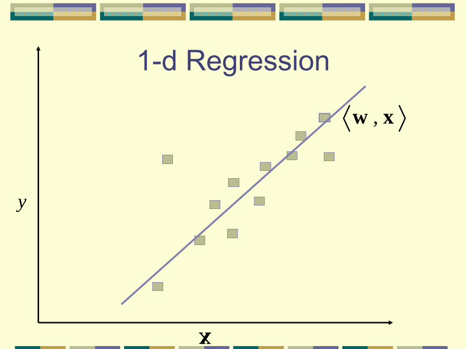
1-d Regression

,w x

y

x

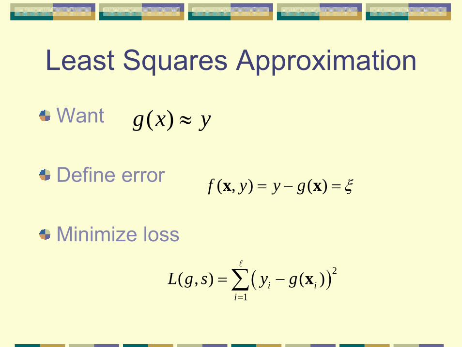
Least Squares Approximation

Want

Define error

Minimize loss

( )g x y≈

( , ) ( )f y y g ξ= − =x x

( )2

1( , ) ( )i i

iL g s y g

=

= −∑ x

“Training” Model

Create function g(x)=x’w that works well on training data as defined by some loss function

For least squares loss this becomes2

1min ( ' )i ii

y=

−∑w x w

1min ( ' , )i ii

loss y=∑w x w

Linear Algebra

Let data matrix X have a data point for each row

Response is vector y

1 2[ , , , ] '=X x x x…

1

2

yy

y

⎡ ⎤⎢ ⎥⎢ ⎥=⎢ ⎥⎢ ⎥⎣ ⎦

y

Equivalent Forms of Loss

21

2

( ) ( ' )

2( ) '( )

2

i iiL y

norm=

= −

= − −

= − −= − +

∑w x w

Xw yXw y Xw y

y'y y'Xw w'X'Xw

Just in time lesson in convex optimization

Convexity and Unconstrained Optimization

WARNING

In Machine Learning Land :x is the datawe minimize loss with respect to the

variable w

In optimization, x is a variablewe minimize objective with respect to x

If you don’t know where you are going, you probably won’t get there.

-from some book I read in eight grade

If you do get there, you won’t know it. -Dr. Bennett’s amendment

Mathematical Programming Theory tells us –How to formulate a model.Strategies for solving the model.How to know when we have found anoptimal solutions.How hard it is to solve the model.

Let’s start with the basics…………………

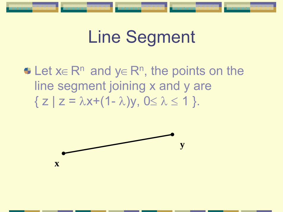
Line Segment

Let x∈Rn and y∈Rn, the points on the line segment joining x and y are { z | z = λx+(1- λ)y, 0≤ λ ≤ 1 }.

y

x

Convex Functions

A function f is (strictly) convex on a convex set S, if and only if for any x,y∈S, f(λx+(1- λ)y)(<) ≤ λ f(x)+ (1- λ)f(y)

for all 0≤ λ ≤ 1.

x y

f(y)

f(x)

x+(1- λ)y

f(x+(1- λ)y)

Concave Functions

A function f is (strictly) concave on a convex set S, if and only if for any –f is (strictly) convex on S.

f -f

(Strictly)Convex, Concave, or none of the above?

None of the above

Concave Convex

Concave Strictly convex

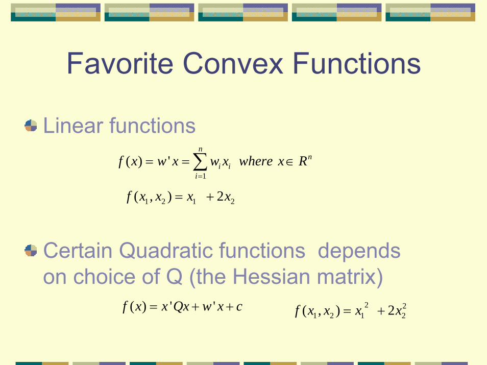
Favorite Convex Functions

Linear functions

Certain Quadratic functions depends on choice of Q (the Hessian matrix)

1( ) '

nn

i ii

f x w x w x where x R=

= = ∈∑

1 2 1 2( , ) 2f x x x x= +

( ) ' 'f x x Qx w x c= + + 2 21 2 1 2( , ) 2f x x x x= +

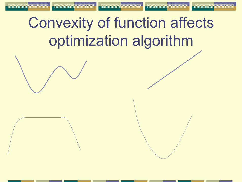
Convexity of function affects optimization algorithm

Theorem 2.1: Global Solution of convex program

If x* is a local minimizer of a convex programming problem, x* is also a global minimizer. Further more if the objective is strictly convex then x* is the unique global minimizer.

Proof. Nash and Sofer

Problems with nonconvexobjective

a x* bf strictly convex, problem has unique global minimum

Min f(x) subject to x ∈ [a,b]

x*f not convex, problem hastwo local minima a x’ b

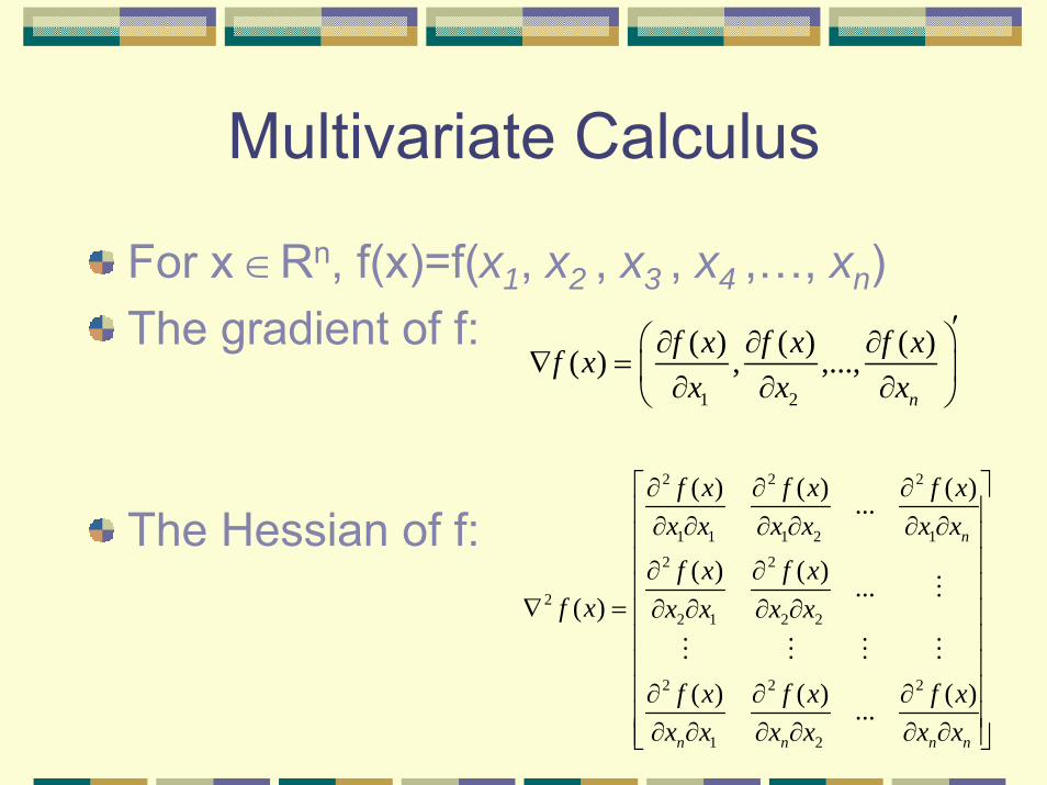
Multivariate Calculus

For x ∈Rn, f(x)=f(x1, x2 , x3 , x4 ,…, xn)The gradient of f:

The Hessian of f:

1 2

( ) ( ) ( )( ) , ,...,n

f x f x f xf xx x x

′⎛ ⎞∂ ∂ ∂∇ = ⎜ ⎟∂ ∂ ∂⎝ ⎠

2 2 2

1 1 1 2 12 2

22 1 2 2

2 2 2

1 2

( ) ( ) ( )...

( ) ( ) ...( )

( ) ( ) ( )...

n

n n n n

f x f x f xx x x x x x

f x f xf x x x x x

f x f x f xx x x x x x

⎡ ⎤∂ ∂ ∂⎢ ⎥∂ ∂ ∂ ∂ ∂ ∂⎢ ⎥⎢ ⎥∂ ∂⎢ ⎥

∇ = ∂ ∂ ∂ ∂⎢ ⎥⎢ ⎥⎢ ⎥⎢ ⎥∂ ∂ ∂⎢ ⎥∂ ∂ ∂ ∂ ∂ ∂⎢ ⎥⎣ ⎦

For example1

1

1

4 321 2 1 2

31 2

32 1

32

22

( ) 3 4

2 3 4( )

1 2 4

2 9 4( )

4 3 6

x

x

x

f x x e x xxx e x

f xx x

ef x

x

= + + +

⎡ ⎤+ +∇ = ⎢ ⎥

+⎢ ⎥⎣ ⎦⎡ ⎤+

∇ = ⎢ ⎥⎣ ⎦

2

[ 0 , 1 ]7

( )1 2

1 1 4( )

4 3 6

x

f x

f x

′=

⎡ ⎤∇ = ⎢ ⎥

⎣ ⎦⎡ ⎤

∇ = ⎢ ⎥⎣ ⎦

Quadratic Functions

Form

Gradient

1 1 1

1( ) '2

12

n n n

i j i j j ji j j

f x x Q x b x

Q x x b x= = =

′= −

= −∑ ∑ ∑

2

( )( )

f x Qx bf x Q

∇ = −∇ =

1

( ) 1 12 2

assuming symmetric

kk k ik i kj j ki k j kk

n

kj j kj

f x Q x Q x Q x bx

Q x b Q

≠ ≠

=

∂= + + −

∂

= −

∑ ∑

∑

n nxn nx R Q R b R∈ ∈ ∈

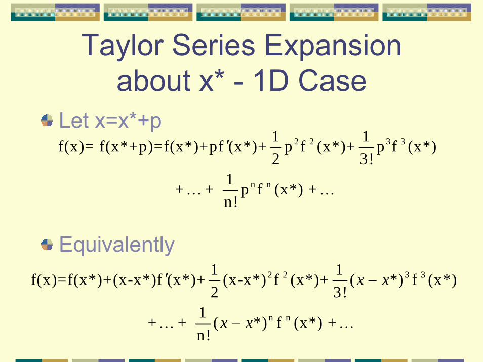
Taylor Series Expansion about x* - 1D Case

Let x=x*+p

Equivalently

2 2 3 3

n n

1 1 f(x)= f(x*+p)=f(x*)+pf (x*)+ p f (x*)+ p f (x*) 2 3!

1 + + p f (x*) +n!

′

… …

2 2 3 3

n n

1 1 f(x)=f(x*)+(x-x*)f (x*)+ (x-x*) f (x*)+ ( *) f (x*) 2 3!

1 + + ( *) f (x*) +n!

x x

x x

′ −

−… …

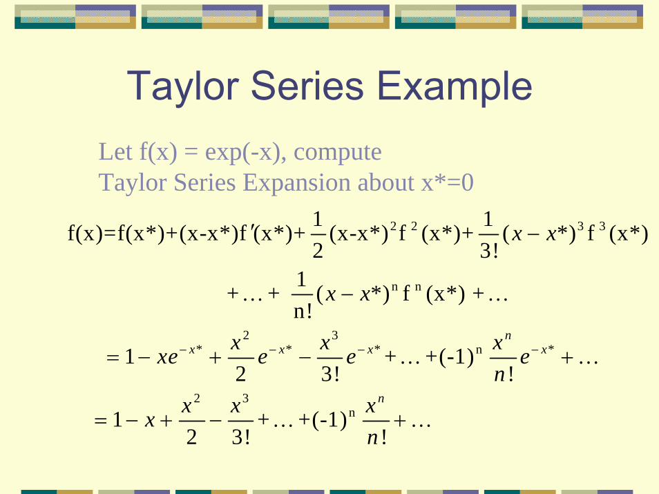
Taylor Series ExampleLet f(x) = exp(-x), compute Taylor Series Expansion about x*=0

2 2 3 3

n n

2 3* * * n *

2 3n

1 1 f(x)=f(x*)+(x-x*)f (x*)+ (x-x*) f (x*)+ ( *) f (x*) 2 3!

1 + + ( *) f (x*) +n!

1 + +(-1)2 3! !

1 + +(-1)2 3! !

nx x x x

n

x x

x x

x x xxe e e en

x x xxn

− − − −

′ −

−

= − + − +

= − + − +

… …

… …

… …

First Order Taylor Series Approximation

Let x=x*+p

Says that a linear approximation of a function works well locally

0

f(x)=f(x*+p)=f(x*)+p f(x*)+ p ( *, )lim ( *, ) 0p

x pwhere x p

αα

→

′∇

=

f(x)f(x)=f(x*+p)= ( *) ( *)f x p f x′+ ∇

x*

f(x)= ( *) ( *) ' ( *)f x x x f x+ − ∇

Exercise

2

3 2 2 21 2 1 1 2 1 2

2 2

( , ) 5 7 2 fu n c t io n

( ) ( * ) [ , ] ' g ra d ie n t

( ) ( * ) H e s s ia n

x x x x x x x

f x f x

f x f x

= + + +

⎡ ⎤∇ =⎢ ⎥

⎣ ⎦⎡ ⎤ ⎡ ⎤

∇ =⎢ ⎥ ⎢ ⎥⎣ ⎦⎣ ⎦

f x

∇ =

∇ =

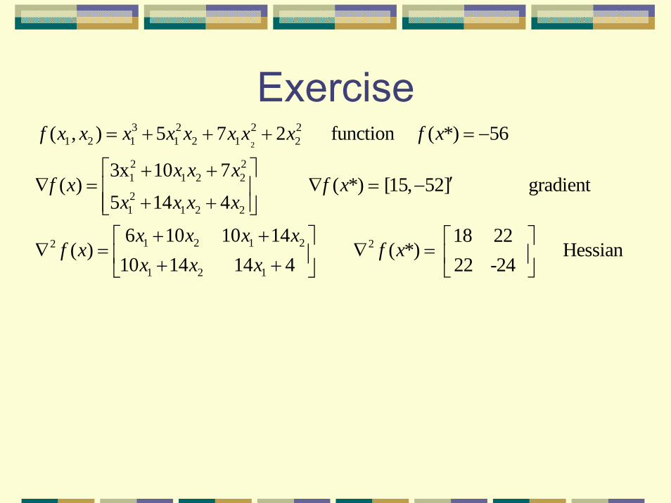
Exercise 2

3 2 2 21 2 1 1 2 1 2

2 21 1 2 221 1 2 2

1 2 1 22 2

1 2 1

( , ) 5 7 2 function ( *) 56

3x 10 7( ) ( *) [15, 52] gradient

5 14 4

6 10 10 14 18 22( ) ( *) Hessian

10 14 14 4 22 -24

f x x x x x x x x f x

x x xf x f x

x x x x

x x x xf x f x

x x x

= + + + = −

⎡ ⎤+ +′∇ = ∇ = −⎢ ⎥

+ +⎢ ⎥⎣ ⎦+ +⎡ ⎤ ⎡ ⎤

∇ = ∇ =⎢ ⎥ ⎢ ⎥+ + ⎣ ⎦⎣ ⎦

Convex Functions

A function f is (strictly) convex on a convex set S, if and only if for any x,y∈S, f(λx+(1- λ)y)(<) ≤ λ f(x)+ (1- λ)f(y)

for all 0≤ λ ≤ 1.

x y

f(y)

f(x)

x+(1- λ)y

f(x+(1- λ)y)

Proving Function Convex

Linear functions

1( ) '

nn

i ii

f x w x w x where x R=

= = ∈∑

, (0,1)( (1 ) ) '( (1 ) )

' (1 ) ' ( ) (1 ) ( )

nFor any x y Rf x y w x y

w x w y f x f yλ λ λ λ

λ λ λ λ

∈ ∈+ − = + −

= + − ≤ + −

Is least squares function convex?

Theorem

Let f be twice continuously differentiable.f(x) is convex on S if and only if for all x∈X, the Hessian at x

is positive semi-definite.

2 ( )f x∇

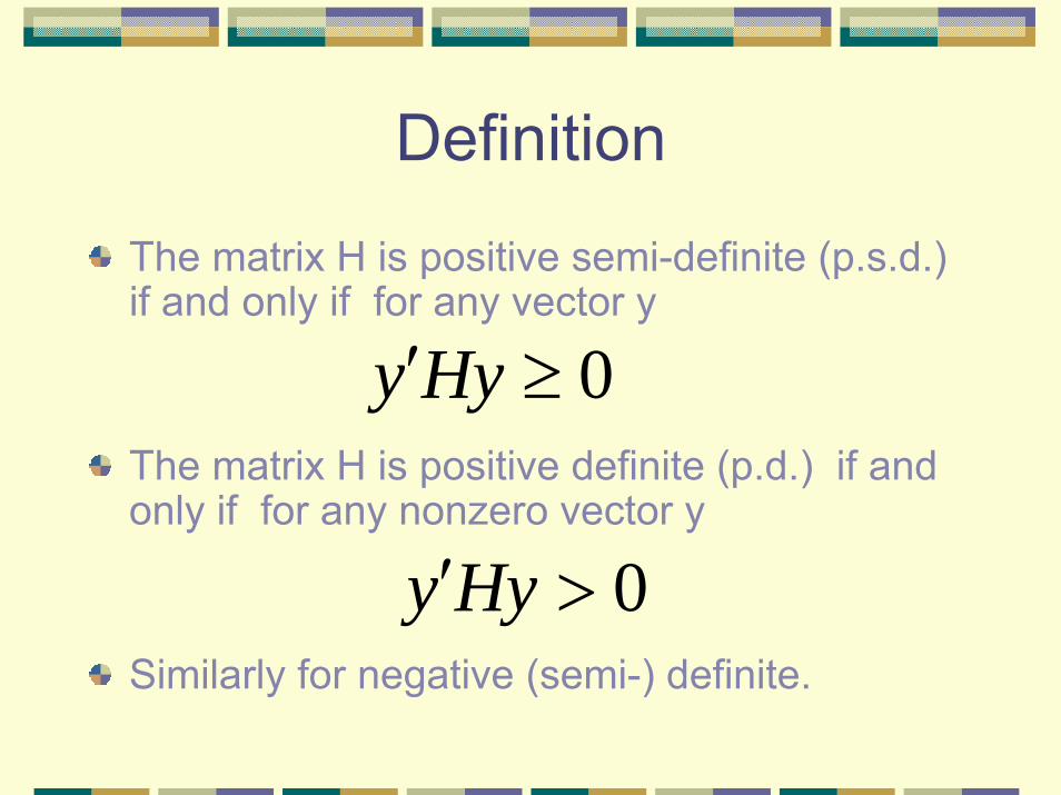
Definition

The matrix H is positive semi-definite (p.s.d.) if and only if for any vector y

The matrix H is positive definite (p.d.) if and only if for any nonzero vector y

Similarly for negative (semi-) definite.

0y Hy′ ≥

0y Hy′ >

Theorem

Let f be twice continuously differentiable.f(x) is strictly convex on S if and only if for all x∈X, the Hessian at x

is positive definite.

2 ( )f x∇

Checking Matrix H is p.s.d/p.d.

Manually

[ ] 1 2 21 2 1 2 1 1 2 2

2

2 21 1 2 2

2 21 2 1 2 1, 2

4 14 3

1 3

4 2 3

( ) ^ 2 3 2 0 [ ] 0so matrix is positive definite

xx x x x x x x x

x

x x x x

x x x x x x

− ⎡ ⎤⎡ ⎤= − − +⎢ ⎥⎢ ⎥−⎣ ⎦ ⎣ ⎦

= − +

= − + + > ∀ ≠

Differentiability and Convexity

For convex function, linear approximation underestimates function

f(x)

( ) ( *) ( *) ( *)g x f x x x f x′= + − ∇

(x*,f(x*))

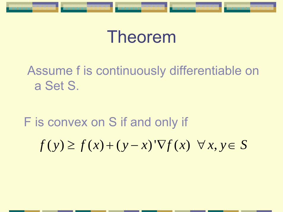
Theorem

Assume f is continuously differentiable on a Set S.

F is convex on S if and only if

( ) ( ) ( ) ' ( ) ,f y f x y x f x x y S≥ + − ∇ ∀ ∈

Theorem

Consider problem min f(x) unconstrained. If and f is convex, then

is a global minimum.Proof:

( ) 0f x∇ =x

( ) ( ) ( ) ' ( ) by convexity of( ) since ( ) 0.

yf y f x y x f x f

f x f x

∀≥ + − ∇= ∇ =

Unconstrained Optimality Conditions

Basic Problem:

(1)

Where S is an open sete.g. Rn

min ( )x S

f x∈

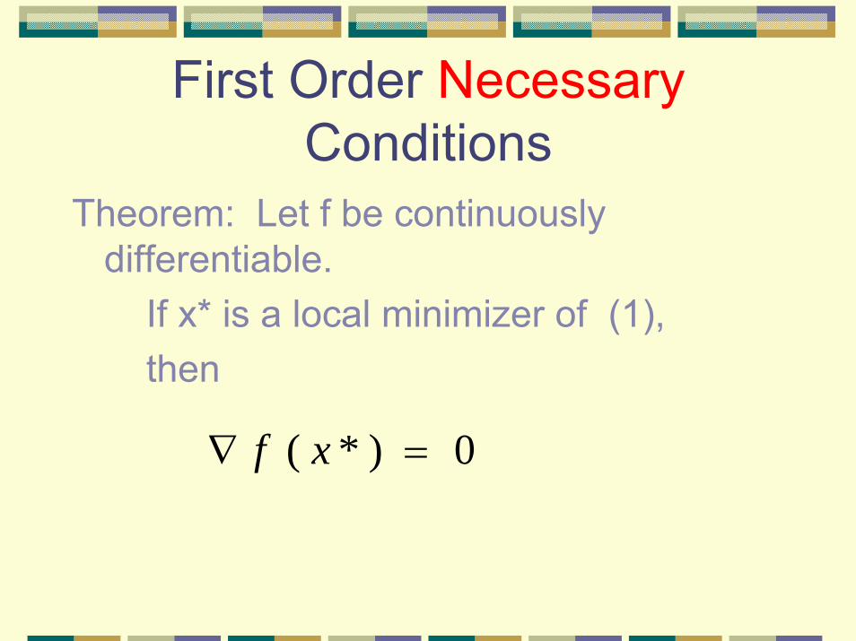
First Order NecessaryConditions

Theorem: Let f be continuously differentiable.

If x* is a local minimizer of (1),then

( * ) 0f x∇ =

Stationary Points

Note that this condition is not sufficient

( * ) 0f x∇ =Also true for

local max and saddle points

Proof

Assume false, e.g.,Let ( *), thend f x= −∇

( * ) ( *) ( *) ( *, )

( * ) ( *) ( *) ( *, )

( * ) ( *) 0 for sufficiently smallsince ( *) 0and ( *, ) 0.

!! * is a local min.

f x d f x d f x d x d

f x d f x d f x d x d

f x d f xd f x x d

CONTRADICTION x

λ λ λ α λ

λ α λλ

λ λα λ

′+ = + ∇ +

⇓+ − ′= ∇ +

⇓+ − <′∇ < →

( *) 0f x∇ ≠

Example

Say we are minimizing 2 2

1 2 1 1 2 2 1 21( , ) 2 15 42

f x x x x x x x x= − + − −

[8,2]???

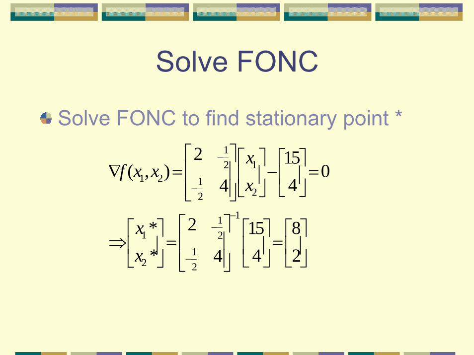
Solve FONC

Solve FONC to find stationary point *1

121 2 1

22

111 2

12 2

2 15( , ) 0

44

2* 15 8* 4 24

xf x x

x

xx

−

−

−−

−

⎡ ⎤⎡ ⎤ ⎡ ⎤∇ = − =⎢ ⎥⎢ ⎥ ⎢ ⎥

⎣ ⎦⎢ ⎥⎣ ⎦⎣ ⎦

⎡ ⎤⎡ ⎤ ⎡ ⎤ ⎡ ⎤⇒ = =⎢ ⎥⎢ ⎥ ⎢ ⎥ ⎢ ⎥

⎣ ⎦ ⎣ ⎦⎢ ⎥⎣ ⎦ ⎣ ⎦

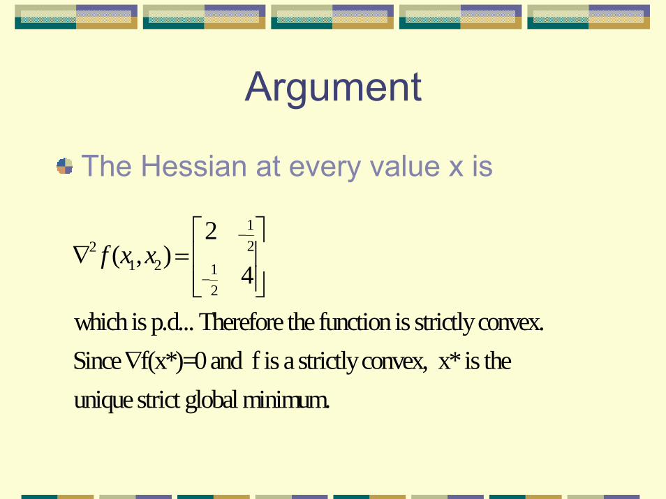
Argument

The Hessian at every value x is

122

1 2 12

2( , )

4

which is p.d... Therefore the function is strictly convex.Since f(x*)=0 and f is a strictly convex, x* is the unique strict global minimum.

f x x−

−

⎡ ⎤∇ =⎢ ⎥

⎢ ⎥⎣ ⎦

∇

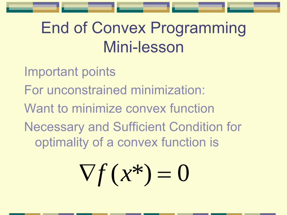
End of Convex Programming Mini-lesson

Important pointsFor unconstrained minimization:Want to minimize convex functionNecessary and Sufficient Condition for

optimality of a convex function is

( *) 0f x∇ =

Least Squares Optimality condition

Find min with respect to w of

21

2

min ( ' )

min 2min ( ) '( )min 2

i iiy or

norm=

−

− −

− −− +

∑ x w

Xw yXw y Xw y

y'y y'Xw w'X'Xw

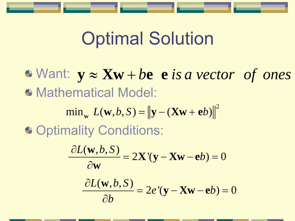
Optimal Solution

Want:Mathematical Model:

Optimality Condition:

Solution satisfies:

( ) ( )2min ( , ) 'L S = − = − −w w y Xw y Xw y Xw

≈y Xw

( , ) 2 ' 2 ' 0L S∂= − + =

∂w X y X Xww

' '=X Xw X y

Solving n×n equation is 0(n3)

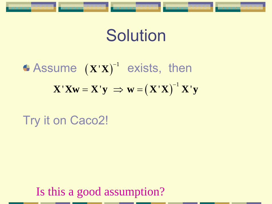
Solution

Assume exists, then

Try it on Caco2!

( ) 1' −X X

( ) 1' ' ' '−= ⇒ =X Xw X y w X X X y

Is this a good assumption?

Ridge Regression

Inverse typically does not exist.Use least norm solution for fixedRegularized problem

Optimality Condition:

2 2min ( , )L Sλ λ= + −w w w y Xw

( , )2 2 ' 2 ' 0

L Sλ λ∂

= − + =∂

ww X y X Xw

w

( )' 'nλ+ =X X I w X y

0.λ >

Requires 0(n3) operations

Generalization

To estimate generalization error:Divide test into training set= Xtrain

100 points in Aquasoland test set = Xtest

97 points in AquasolCreate g(x) using XtrainEvaluate on Xtest

Matlab

Matlab command:

Train and Test for λ

0.5 1 1.5 2 2.5 3 3.5 4 4.5 5

0

2

4

6

8

10

12

14

16

x

trainerr(x)

0.5 1 1.5 2 2.5 3 3.5 4 4.5 51.5

1.55

1.6

1.65

1.7

1.75

1.8

1.85

1.9

1.95

x 104

x

testerr(x)

1-d Regression with bias

, b+w x

x

y

b=2

Optimal Solution

Want:Mathematical Model:

Optimality Conditions:

2min ( , , ) ( )L b S b= − +w w y Xw e

b is a vector of on≈ +y Xw e e

( , , ) 2 '( ) 0L b S b∂= − − =

∂w X y Xw e

w( , , ) 2 '( ) 0L b S e b

b∂

= − − =∂w y Xw e

es

Optimal Solution

Thus :

Idea: Scale data so means are 0, e.g

' ' '' ' ( ) ( ) '

b

b mean mean

= −

⇒ = − = −

e e e y e Xwe y e Xw y X w

' ' ' b= −X Xw X y X e

' 0' 0==

e ye X

Recenter Data

Shift y by mean

Shift x by mean

1

1 :i i ii

y y yµ µ=

= = −∑

1

1 :i i ii=

= = −∑x x x x x

Ridge Regression with bias

Recenter X and y by Find least squares solution

How do you predict a new point?

x and µ

1( ) 'λ −= +w X'X I X y

( )f =x x'w

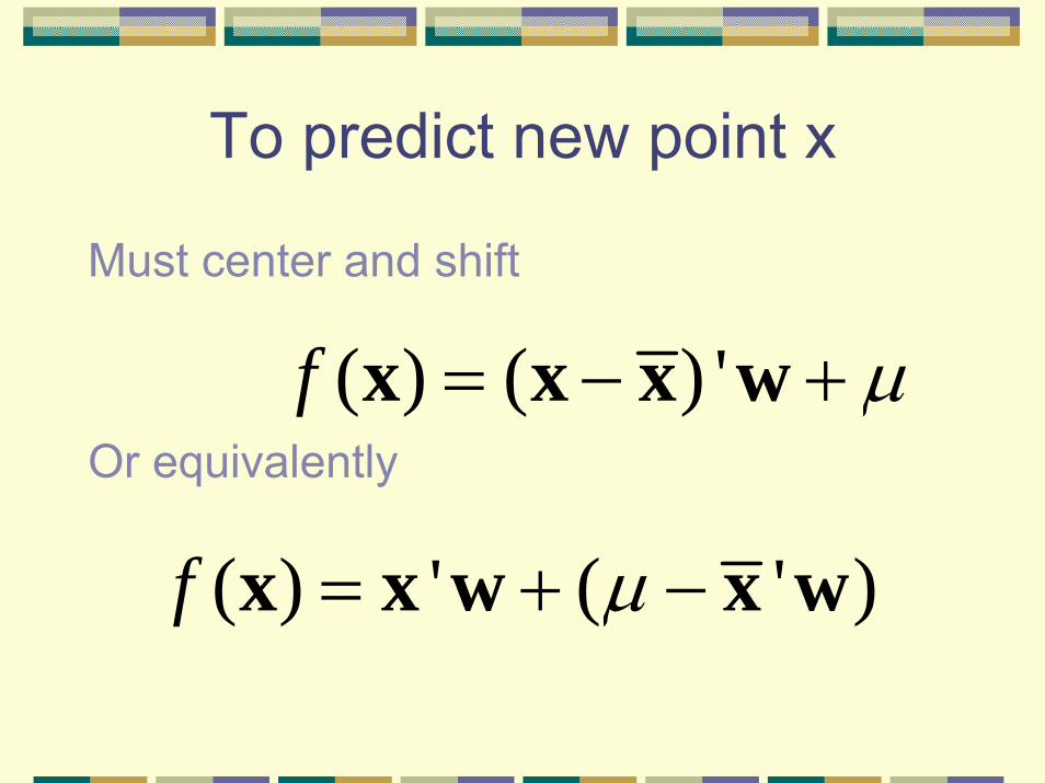
To predict new point x

Must center and shift

Or equivalently( ) ( ) 'f µ= − +x x x w

( ) ' ( ' )f µ= + −x x w x w

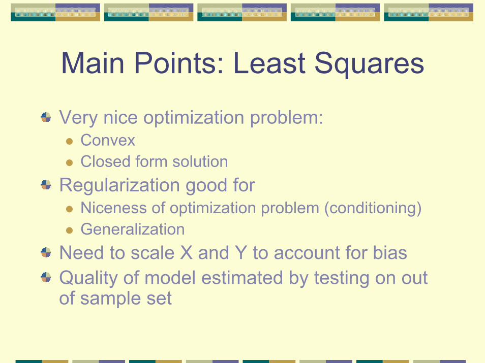
Main Points: Least Squares

Very nice optimization problem:ConvexClosed form solution

Regularization good forNiceness of optimization problem (conditioning)Generalization

Need to scale X and Y to account for biasQuality of model estimated by testing on out of sample set

Limitations?

Will this model work on all drug discovery models?

Next Class

Alternative losses and regularization based on 1-norm regularizationJust in time linear programming

Nonlinear Regression