Regress™ User’s Guide

Jeffrey H. MooreGraduate School of Business, Stanford University

IntroductionA statistical regression add-in to Microsoft Excel on Macintosh

and Windows computers, Regress1 makes exploratory regression analysis fast and convenient. It does this by displaying preliminary results in a temporary window that you can easily dismiss during the exploratory modeling phase. This allows you to run many regression models, interactively adding and dropping variables, as you evaluate alternative models for reasonableness and goodness-of-fit.

Since Regress is an add-in to Excel, you have all the normal Excel worksheet capabilities available. This includes, for example, the ability to cut and paste the results into another Excel worksheet, Microsoft Word document, or other Windows or Macintosh compatible application. Moreover, you have complete freedom to change the formatting, the fonts, the size of tables and charts, etc., to suit your particular requirements. This flexibility is rarely present in other dedicated regression packages.

I Tutorial

Getting Started with RegressTo begin, launch Excel as usual.2 Regress should appear as the

last item on the "Tools" menu. See the figure below, left. If you do not see “Regress” listed, it has not been properly installed on your computer (or, if you purchased Regress, you neglected to re-start Excel after installing it on your computer.)

Now, click the “Regress” item on the Tools menu, causing Regress to be loaded into Excel as an Add-In. During the load process,

1 © Copyright Sept., 1999 This manual documents Version 1.8a of Regress for Excel Ver. 98 for Macintosh (System 8+) and Excel Ver. 97/2000 for Windows PC's (Windows 95/98/NT). The Regress software is available from Nexus Systems, P.O. Box 20075, Stanford CA 94309-20075.

2 Macintosh users: Excel on Macintosh defaults to a too small memory partition for Excel yielding a severe response time penalty caused by virtual mem ory swaps to disk for large Add-Ins, such as Solver or Regress. Macintosh Excel users should increase Excel's default memory allocation by an additional 1 megabyte or more as Excel’s “Preferred Size,” i.e., click the Microsoft Excel application icon and press Command-i to display and change Macintosh Excel's preferred memory size require -ment.

2you should see three changes:(1) Excel will ask if you wish to allow a macro add-in to be opened.

Click “Enable Macros” to begin. (2) A herald window will remind you that you need to open a

workbook containing your data. (See the figure below, right.)(3) Finally, a small toolbar entitled “Regress,” containing three but-

tons, will appear in the upper right corner of your screen. (See the small figure below.)

When the herald window closes, loading of Regress is

complete. Regress will remain loaded into Excel and available until you quit Regress by clicking the “Q” button. Normal spreadsheet functions are unaffected by Regress, and you can use Excel as usual. Since its only function is to initiate loading, the “Regress” item on the Tools menu is removed after the Regress Toolbar appears. Thereafter, all regression modeling is done by clicking each of the three Regress Toolbar buttons, the middle one of which is not yet defined.

The Regress Toolbar “floats” above all Excel windows, and as with any Excel toolbar, you may move it out of the way or dock it by click-dragging its title bar.3

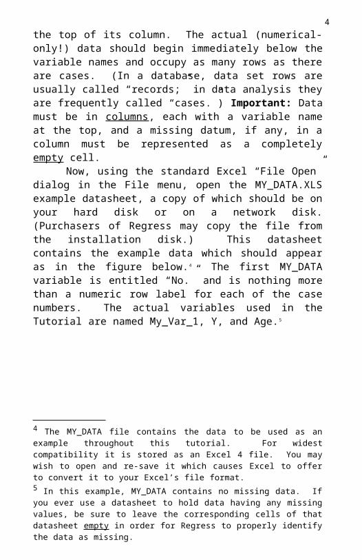
A sheet within a workbook containing the data for your regression modeling is called a Regress “datasheet” in this User’s Guide. The topmost row in any Regress datasheet is a special row containing each variable’s name at the top of its column. The actual (numerical-only!) data should begin immediately below the variable names and occupy as many rows as there are cases. (In a database, data set rows are usually called “records;” in data analysis they are frequently called “cases.”) Important: Data must be in columns, each with a variable name at the top, and a missing datum, if any, in a

3 Closing the Regress toolbar by clicking its or un-checking it in the View\Toolbars menu, causes it to be hidden. To un-hide it, select the Toolbars item on the View menu, then click Regress in the Toolbar sub-menu..

3column must be represented as a completely empty cell.

Now, using the standard Excel “File Open” dialog in the File menu, open the MY_DATA.XLS example datasheet, a copy of which should be on your hard disk or on a network disk. (Purchasers of Regress may copy the file from the installation disk.) This datasheet contains the example data which should appear as in the figure below. 4

The first MY_DATA variable is entitled “No.” and is nothing more than a numeric row label for each of the case numbers. The actual variables used in the Tutorial are named My_Var_1, Y, and Age.5

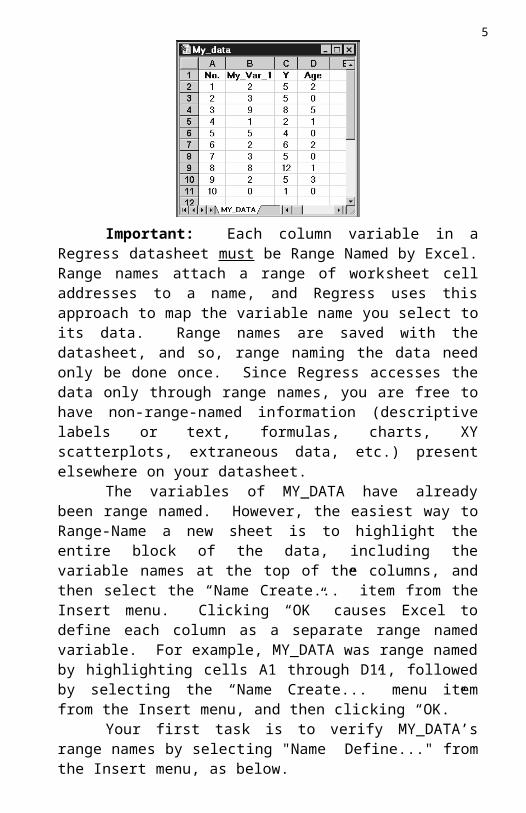
Important: Each column variable in a Regress datasheet must be Range Named by Excel. Range names attach a range of worksheet cell addresses to a name, and Regress uses this approach to map the variable name you select to its data. Range names are saved with the datasheet, and so, range naming the data need only be done once. Since Regress accesses the data only through range names, you are free to have non-range-named information (descriptive labels or text, formulas, charts, XY scatterplots, extraneous data, etc.) present elsewhere on your datasheet.

The variables of MY_DATA have already been range named. However, the easiest way to Range-Name a new sheet is to highlight the entire block of the data, including the variable names at the top of the columns, and then select the “Name Create...” item from the Insert menu. Clicking “OK” causes Excel to define each column as a separate range named variable. For example, MY_DATA was range named by highlighting cells A1 through D11, followed by selecting the “Name Create...” menu item from the Insert menu, and then clicking “OK.”

Your first task is to verify MY_DATA’s range names by 4 The MY_DATA file contains the data to be used as an example throughout this tutorial. For widest compatibility it is stored as an Excel 4 file. You may wish to open and re-save it which causes Excel to offer to convert it to your Excel’s file format.5 In this example, MY_DATA contains no missing data. If you ever use a datasheet to hold data having any missing values, be sure to leave the corresponding cells of that datasheet empty in order for Regress to properly identify the data as missing.

4selecting "Name Define..." from the Insert menu, as below.

As seen in the Define Name dialog box below, you can verify the range for any variable by clicking its name and noticing the range of cells to which that name refers. For example, the name “My_Var_1” has been assigned the range of cells B2 through B11. (Always verify that the variables in your datasheet have the proper ranges associated with them. Otherwise, Regress may not process all your data!) After reviewing the variable ranges, click “OK” to close the Define Name dialog box.

At this point, you should have the Regress Toolbar showing on your screen and have your properly ranged-named datasheet, MY_DATA, opened in Excel. For simplicity, there should be no other workbooks open except your datasheet.6

Now you are ready to begin exploratory regressions.

Exploratory Regression Analysis

Be sure your datasheet is open, and click the left “Regression” button

on the Regress Toolbar.

Clicking the left button on the Regress Toolbar always displays the Exploratory Regression dialog box, as below. Displayed 6 If you do have multiple workbooks open, Regress will ask you to select the one to use for your datasheet. Make sure the active sheet in the workbook is your datasheet.

5on the left is an alphabetic list of all the range-named variables in your open datasheet.7

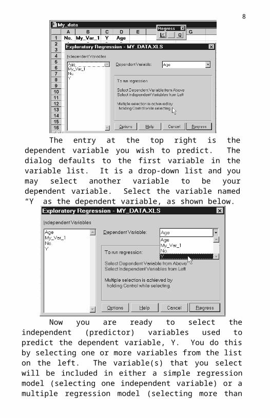
The entry at the top right is the dependent variable you wish to predict. The dialog defaults to the first variable in the variable list. It is a drop-down list and you may select another variable to be your dependent variable. Select the variable named “Y” as the dependent variable, as shown below.

Now you are ready to select the independent (predictor) variables used to predict the dependent variable, Y. You do this by selecting one or more variables from the list on the left. The variable(s) that you select will be included in either a simple regression model (selecting one independent variable) or a multiple regression model (selecting more than one independent variable). For now, select the variable Age as the single independent variable you will use to predict

7 Actually, Regress will display all the range named variables from all sheets in your workbook. To avoid confusion, it is best to define workbook range names only for the data in your datasheet. That is, range names in an Excel workbook are global, i.e., defined across all its worksheets. Therefore, it is a good idea to place each datasheet in a separate workbook with no other defined names.

6values of Y. See below.

Next, click the button to cause the (simple) regres-sion model to be fit to the data. Regress will open a new Excel work-book called “Exploratory Results,” shown below. By default, Exploratory Results displays the names of the dependent and in-dependent variable(s) and two summaries, the “Regression Statistics” and the “Summary Table.”8

The Regression Statistics gives information about your model’s goodness of fit (signaled by the Adjusted R-square, “Adj.RSqr”), the Standard Error of the Regression, “Std.Err.,”9 the number of cases used, “# Cases,” and number of cases dropped because of missing data, “#Missing,” if any.

The Summary Table gives the coefficients of the regression model, “Coeff.,” along with their standard errors, “Std.Err.,” and the resulting statistics, “t-Stat.” and “P-value,” used for hypothesis tests on the coefficients.

At the top of the Exploratory Results window are two buttons that you may click for additional information: Help gives a brief summary of your options.

8 The Options button in the Exploratory Regression dialog box permits you to change the default summaries and the number of decimal digits displayed.9Also known as the “Standard Deviation of the Residuals” or “Standard Error of the Estimate.”

7 Correlation presents the correlation matrix among all the pairs of

variables in your model.

Because it is just another worksheet, you are free to open new windows and do other work even though the Exploratory Results window is open. Also, you can save Exploratory Results to disk or print it, if you wish. However, these are not its intended functions. Rather, Exploratory Results presents preliminary information about your regression model that you will either dismiss immediately in favor of another model or keep in a more detailed report worksheet.

Keeping a Regression ModelWhen the Exploratory Results window appears, a change oc-

curs in the Regress Toolbar buttons. All three buttons become defined, as shown on the right.

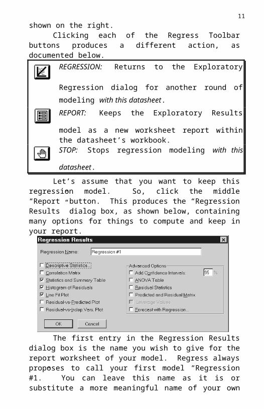
Clicking each of the Regress Toolbar buttons produces a different action, as documented below.

REGRESSION: Returns to the Exploratory Regression dialog

for another round of modeling with this datasheet.

REPORT: Keeps the Exploratory Results model as a new

worksheet report within the datasheet’s workbook.

STOP: Stops regression modeling with this datasheet.

Let’s assume that you want to keep this regression model. So, click the middle “Report” button. This produces the “Regression Results” dialog box, as shown below, containing many options for things to compute and keep in your report.

The first entry in the Regression Results dialog box is the

8name you wish to give for the report worksheet of your model. Regress always proposes to call your first model “Regression #1.” You can leave this name as it is or substitute a more meaningful name of your own choosing.10.

Change the dialog box’s Regression Name to be “My Regression Model.” You may now select the tables and plots that you would like to save, including if you wish, the Exploratory Results information Regress previously calculated. So, click the Descriptive Statistics option. This will produce another dialog box listing some standard statistics for your variables, as below. These statistics are not regression model statistics, but are computed from your raw data for possible comparisons later with your regression model results.11

Accept these defaults by clicking the “OK” button, returning you to the “Regression Results” dialog box.

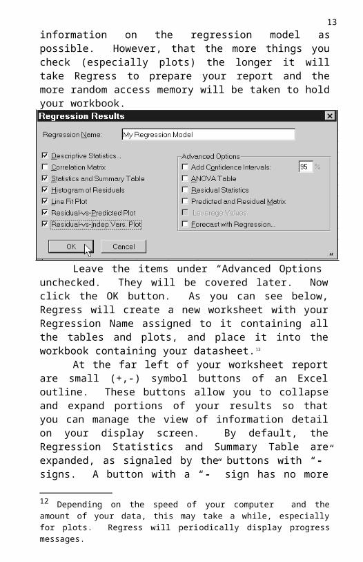
Now, click the boxes to keep the items shown in the dialog below. You need not collect all this information. Of course, you can always check everything to get as much information on the regression model as possible. However, that the more things you check (especially plots) the longer it will take Regress to prepare your report and the more random access memory will be taken to hold your workbook.

10 The Regression Name may be up to 31 characters long and may contain spaces.11 The Descriptive Statistics are computed after dropping cases containing missing data, if any, for the variables in your model. These statistics may differ from those produced by similar Excel statistical functions applied to your datasheet that do not consider dropped cases.

9

Leave the items under “Advanced Options” unchecked. They will be covered later. Now click the OK button. As you can see below, Regress will create a new worksheet with your Regression Name assigned to it containing all the tables and plots, and place it into the workbook containing your datasheet.12

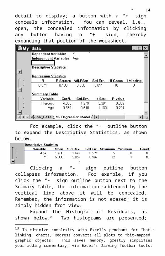
At the far left of your worksheet report are small (+,-) symbol buttons of an Excel outline. These buttons allow you to col lapse and expand portions of your results so that you can manage the view of information detail on your display screen. By default, the Regression Statistics and Summary Table are expanded, as signaled by the buttons with “-” signs. A button with a “-” sign has no more detail to display; a button with a “+” sign conceals information. You can reveal, i.e., open, the concealed information by clicking any button having a “+” sign, thereby expanding that portion of the worksheet.

12 Depending on the speed of your computer and the amount of your data, this may take a while, especially for plots. Regress will periodically display progress messages.

10For example, click the “+” outline button to expand the

Descriptive Statistics, as shown below.

Clicking a “-” sign outline button collapses information. For example, if you click the “-” sign outline button next to the Summary Table, the information subtended by the vertical line above it will be concealed. Remember, the information is not erased; it is simply hidden from view.

Expand the Histogram of Residuals, as shown below.13 Two histograms are presented; the darker (red) bars are the actual residuals from the model, and the lighter (blue) bars give the height of the theoretical bell-shaped normal curve that you would expect from normally distributed residuals. This allows you to compare visually the shape of the theoretical and the actual frequency histograms to see if the results violate the “normal distribution of residuals” assumption for a regression model.14

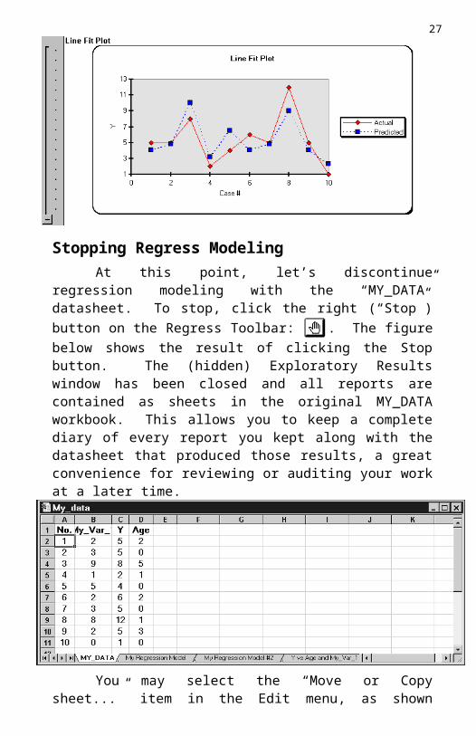
Next, collapse the Histogram of Residuals and expand the Line Fit Plot., as shown below.

13 To minimize complexity with Excel’s penchant for “hot-linking” charts, Regress con-verts all plots to “bit-mapped” graphic objects. This saves memory, greatly simplifies your adding commentary, via Excel’s Drawing Toolbar tools, and cutting/pasting your results into other applications, such as Word. However, it does mean that the only editing of plots you can do is for a bit-mapped graphic object (scaling the picture, adding borders, etc.).14 Excel defaults all charts to have a gray background. This produces a prettier ap-pearance of the chart on color displays. However, this can lead to loss of contrast on monochrome displays, such as on many laptop computers, or poor quality black and white printing. Section III describes how to change the background default for charts.

11

Whenever you define a “simple”

regression model, the Line Fit Plot shows the Predicted-Y verses Age regression line itself with the scatter of Actual-Y values around it. (This plot is not possible for models with more than one predictor variable.) The vertical distance between the Actual-Y values and the regression line is the “Residual” or “Error” value for that case, given your current regression model.

Now, collapse the Line Fit Plot and expand the Residual Plots. Notice that two-level outlining is used advantageously for nesting the Residual Plots. You can expand and collapse each of these residual scatter plots by clicking its outline button or collapse all of them as a group.15

Click the outline buttons to expand the “Residuals -vs- Predicted Plot,” and the “Age Residual Plot,” as shown below.

15 In general, collapsing plots and tables which are not of immediate interest speeds Excel screen updating when scrolling, and conveniently, also restricts those items from being printed, saving time and paper.

12

Don’t forget that every Regress produced report is an entry in your datasheet’s workbook and is an Excel worksheet with its gridlines and row/column entries turned off. You can change fonts and number formats, copy/paste, annotate, etc., at will.

This completes your first regression model. Now is a good time to save your workbook. So, select the “Save” or “Save As” item from the File menu. Excel will prompt to convert MYDATA.XLS to workbook format during the Save operation. If you do not convert it to a workbook, Excel will save only the active worksheet and not the entire workbook.

How do you go back to create other regression models from this datasheet using different variables? You do this at any time by clicking the left button on the Regress Toolbar. At this point, you have several other options, however.

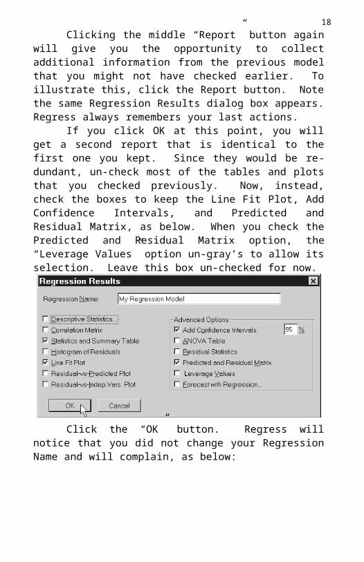
Clicking the middle “Report” button again will give you the opportunity to collect additional information from the previous model that you might not have checked earlier. To illustrate this, click the Report button. Note the same Regression Results dialog box appears. Regress always remembers your last actions.

If you click OK at this point, you will get a second report that is identical to the first one you kept. Since they would be redundant, un-check most of the tables and plots that you checked previously. Now, instead, check the boxes to keep the Line Fit Plot, Add Confidence Intervals, and Predicted and Residual Matrix, as below.

13When you check the Predicted and Residual Matrix option, the “Leverage Values” option un-gray’s to allow its selection. Leave this box un-checked for now.

Click the “OK” button. Regress will notice that you did not change your Regression Name and will complain, as below:

Since you are asking for more information on the same regres-sion model, normally, you would “Append” the new information to the previous report worksheet. However, for the sake of illustration, let’s keep this second report in a separate worksheet. So, click the third option (“Save results instead to:”) to place the report into a second worksheet whose name defaults to an incremented version of the previous name, which you can override, if you wish, with another name. For now, accept the new default name by clicking the OK button.

Regress opens a new worksheet using the name of “My Regression Model #2.” Contained in it is a new Statistics and Summary Table, Line Fit Plot, and the Residual Table. Whenever the

14advanced option “Add Confidence Intervals” is checked, Regress also produces three additional statistics in the Statistics and Summary Table: (1) the regression model’s degrees of freedom, “Deg.Free,” and using the degrees of freedom and the default 95% option, (2) the “back-of-statistics-book” t-table value for a two tail, (1-95%)/2 = 2.5%, hypothesis test, “t(2.5%, 8).” In addition, (3) the 95% confidence intervals are presented for each regression coefficient.

Next, expand the Line Fit plot. Whenever you define a one-predictor regression model and check the “Add Confidence Intervals” option, Regress also adds the 95% confidence interval lines for forecasting the range of individual population values of Y given Age.16

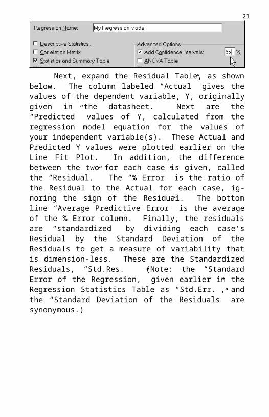
In all appropriate tables and plots, such as above, you may, of course, override the 95% default Regress uses by changing the “95%” entry in the earlier dialog box, repeated below.

16 The confidence interval given in the plot is for the distribution of the individual population values of Y given Age, not for the distribution of the mean of Y given Age.

15

Next, expand the Residual Table, as shown below. The column labeled “Actual” gives the values of the dependent variable, Y, originally given in the datasheet. Next are the “Predicted” values of Y, calculated from the regression model equation for the values of your independent variable(s). These Actual and Predicted Y values were plotted earlier on the Line Fit Plot. In addition, the difference between the two for each case is given, called the “Residual.” The “% Error” is the ratio of the Residual to the Actual for each case, ignoring the sign of the Residual. The bottom line “Average Predictive Error” is the av-erage of the % Error column. Finally, the residuals are “standardized” by dividing each case’s Residual by the Standard Deviation of the Residuals to get a measure of variability that is dimension-less. These are the Standardized Residuals, “Std.Res.” (Note: the “Standard Error of the Regression,” given earlier in the Regression Statistics Table as “Std.Err.”, and the “Standard Deviation of the Residuals” are synonymous.)

The figure to the right shows an alternative way to select among any windows that are open by using the Window menu. Notice

16that your workbook is the only (un-hidden) window open at this point. The two kept model report worksheets, or more precisely, two worksheets of information about the same regression model, are sheets inside the workbook. Also, note that the “Unhide...” option on the Window menu is not grayed out. Regress has hidden the Exploratory Results worksheet to speed computation by eliminating the time to update its screen image.

Let’s try a different regression model on the same datasheet. So, “dismiss” the current model by pressing the left Regress Toolbar button, thereby returning to the Exploratory Regression dialog box, as shown below. Regress preserves the original selection of variables, and you can now choose a different dependent variable or a new subset of independent variables.

This time, select “Age” and “My_Var_1” as two predictor vari-ables. You select several independent variables by holding down the Ctrl key (Windows), or Command key (Macintosh), and clicking each variable name. Now, click the Regress button to start the process again. The Exploratory Results window will be un-hidden and updated to present the results of the new (multiple) regression model, as shown below.

17At this point, let’s compare this two-predictor-variable

multiple regression model with the simple one-predictor-variable regression previously saved in your workbook. Since all Regress produced information is in Excel worksheets, you can display multiple windows at any time. So, click the “My Regression Model” tab in the workbook to compare visually the previous model’s results with the new ones in Exploratory Results.

The figure below shows the result of going back to the workbook and comparing the old model with the new one. If your display screen is large enough, you can move the workbook window below or to the side of Exploratory Results to compare continuously new exploratory models against earlier results.

Now, go back to Exploratory Results by clicking on its window title bar (or using the Window menu). Let’s keep a report for the two predictor variable model. So, click the middle “Report” button on the Regress Toolbar to get the Regression Results dialog box with a proposed name for your, in this case, third worksheet report. Since this is an entirely new model, you should override the proposed name. Give the model a more meaningful name, “Y vs. Age and My_Var_1,” and select the items to keep, as shown in the figure below.

18

Click “OK” to get the worksheet report for this new model, as shown below. Notice that the “Y vs. Age and My_Var_1” model has become another sheet in your workbook. You now have four sheets in the workbook (a datasheet and three regression reports), completely documenting all of your work in this modeling session for future perusal or printing.

Expand the Correlation Matrix table to see the simple cor-relation between any two pairs of variables. This is useful for spotting any (first-order) collinearity among the independent (predictor) variables.

Next, expand the Residual Table. Note the smaller Average Predictive Error percentage produced by the higher R-Square results of this two variable regression model.

19

Next, expand the Line Fit Plot. Notice that it has changed from that of the simple regression model shown earlier. Since, the re-gression “line” cannot be plotted for regression models with more than one predictor variable on a two dimensional plot, the Line Fit Plot changes to plotting the Actual-Y and Predicted-Y (as calculated in the Residual Table above) for each of the cases.

Stopping Regress ModelingAt this point, let’s discontinue regression modeling with the

“MY_DATA” datasheet. To stop, click the right (“Stop”) button on the Regress Toolbar: . The figure below shows the result of clicking the Stop button. The (hidden) Exploratory Results window has been closed and all reports are contained as sheets in the original MY_DATA workbook. This allows you to keep a complete diary of every report you kept along with the datasheet that produced those results, a great convenience for reviewing or auditing your work at a later time.

20

You may select the “Move or Copy sheet...” item in the Edit menu, as shown below, if you prefer to keep your datasheet or any particular worksheet report in a separate workbook.

Notice that after clicking “Stop,” the Regress Toolbar changes its appearance again. Since there is no exploratory model now, the middle “Report” button becomes blank. To resume regression modeling later in the Excel session, open a workbook, select a datasheet (with Range-Named variables!), and click the left “Regression” button on the Regress Toolbar.

The figure below shows the Select Datasheet dialog box that Regress may offer when you click the left button. In this example, two workbooks happen to be open simultaneously, and Regress is asking you which datasheet to use: the one you originally opened, MY_DATA.XLS, or another open one called “Companys.xls.” Optionally, you may click the Open button to open another previously saved workbook.

21

If you were interested in the data from COMPANYS, you would select it and click the OK. Regress would then produce the Exploratory Regression dialog box for that datasheet. You can, therefore, have several datasheet workbooks open at once. However, during your modeling, Regress must then ask you to remove ambiguity by selecting the datasheet of interest. You can avoid this dialog by closing all but the one workbook of interest.Quitting Regress

After stopping Regress, the right “Stop” button in the Regress Toolbar changes to a to allow you to completely “Quit” from the Regress application. Clicking the “Q” button frees primary memory by removing the Regress add-in software from the Excel workspace and deleting the Regress Toolbar. Quitting enables the Regress item in the Tools menu to allow re-loading Regress at a later time.

If you quit from Excel now, Excel will verify if the workbook has been saved recently to the hard disk and may offer you the usual “File Save” dialog in which you can give the workbook a more meaningful name. To be safe, you should periodically select the “Save” item under the File menu to keep a running backup of your results.

As shown below, the workbook, including all its worksheet entries, will be saved under the name “My_Work.” (Under Windows: My_Work.xls) Now you can quit Excel or open another workbook, at your option.

22

Technical LimitationsUse of Regress within Excel is governed by two important limitations:

1. It is common to forget how many tables and charts you end up “keeping” into a workbook during a Regress modeling session. It is easy to accumulate ten or more regression model worksheet reports, each with a dozen charts or more. Ten worksheets and 120+ charts is a sizable chunk of primary memory for Excel to handle, especially for larger data sets. If you wait to get Excel’s “Out of Memory” message, it may be too late to save your work-book! This is especially true for Windows, as its internal User/GDI system resources memory is of fixed size and is used up quickly by the graphics even if you have lots of RAM or Windows swap file space on your hard disk. So, save your workbook often!

2. Regress is limited by restrictions within Excel to no more than 16 variables in any one regression model and to no more than 250 cases.

ConclusionThere are many more useful options available in Regress that

have not been covered in this initial tutorial section. For example, you are always free at any time to perform non-linear regression modeling or to use the Chart Wizard to produce scatter plots for your raw data. These are only two examples of the almost unlimited flexibility Regress coupled with Excel offers in your regression modeling. The following three sections elaborate on these and other more advanced options in Regress, and additional tips and techniques, including non-linear regression modeling, that you will find useful. There is also an important fourth section on Problems and Error Messages that you will find useful.

This tutorial section has given you an introduction to ex-ploratory regression analysis with Regress. As you see from this brief

23summary, the Excel base Regress builds upon makes it quite flexible and very convenient for developing your final regression model. Most likely, this spreadsheet foundation is Regress’ most endearing capability. Good luck with regression modeling and...

“May the High R-Square Be With You.”

24

II Advanced Regress ReportingThe Regression Results dialog allows several other options for

you to add to the report for your model: Analysis of Variance (ANOVA) Table, Residual Statistics, Leverage Values, and Forecast with Regression, as checked below.

Analysis of VarianceThe ANOVA table summarizes the regression model equation

into an F statistic. The P-value associated with this statistic allows test of the overall significance of the regression model apart from the significance, if any, of the equation's individual regression coefficients. For example, extreme multi-collinearity could produce a Regression Summary report with few or no significant regression coefficients, even though the overall regression model has high predictive value (high adjusted R-square statistic). High predictive value of the model would be signaled by an F statistic with low P-value. Loosely speaking, the P-value of the F statistic tests the overall adjusted R-square value, "Adj.RSqr," as being significantly different from zero, i.e., that at least one regression coefficient is significantly different from zero.

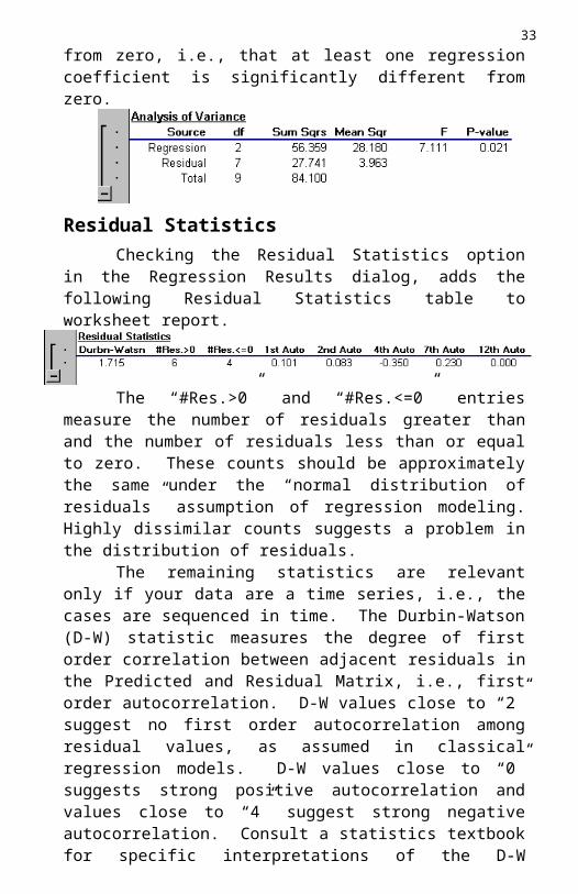
Residual StatisticsChecking the Residual Statistics option in the Regression

Results dialog, adds the following Residual Statistics table to worksheet report.

The “#Res.>0” and “#Res.<=0” entries measure the number of

25residuals greater than and the number of residuals less than or equal to zero. These counts should be approximately the same under the “normal distribution of residuals” assumption of regression modeling. Highly dissimilar counts suggests a problem in the distribution of residuals.

The remaining statistics are relevant only if your data are a time series, i.e., the cases are sequenced in time. The Durbin-Watson (D-W) statistic measures the degree of first order correlation between adjacent residuals in the Predicted and Residual Matrix, i.e., first order autocorrelation. D-W values close to “2” suggest no first order autocorrelation among residual values, as assumed in classical regression models. D-W values close to “0” suggests strong positive autocorrelation and values close to “4” suggest strong negative autocorrelation. Consult a statistics textbook for specific interpretations of the D-W statistic and more formal hypothesis testing using it. The other statistics in the table measure the Autocorrelation between the residuals and the appropriately lagged, i.e., non-adjacent, residuals in case there are cyclic patterns in the residuals, such as monthly (4th Auto for weekly data), weekly (7th Auto for daily data), or yearly (12th Auto for monthly data)Leverage Values

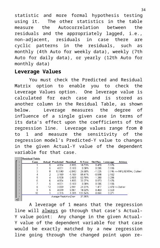
You must check the Predicted and Residual Matrix option to enable you to check the Leverage Values option. One leverage value is calculated for each case and is stored as another column in the Residual Table, as shown below. Leverage measures the degree of influence of a single given case in terms of its data's effect upon the coefficients of the regression line. Leverage values range from 0 to 1 and measure the sensitivity of the regression model's Predicted-Y value to changes in the given Actual-Y value of the dependent variable for that case.

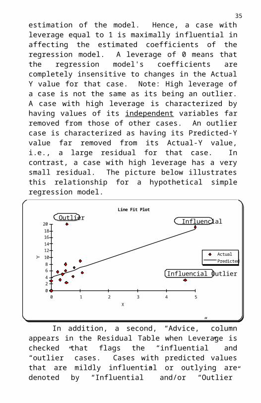
A leverage of 1 means that the regression line will always go through that case’s Actual-Y value point: Any change in the given Actual-Y value of the dependent variable for that case would be exactly matched by a new regression line going through the changed point upon re-estimation of the model. Hence, a case with leverage equal to 1 is maximally influential in affecting the estimated coefficients of the regression model. A leverage of 0 means that the

26regression model's coefficients are completely insensitive to changes in the Actual Y value for that case. Note: High leverage of a case is not the same as its being an outlier. A case with high leverage is characterized by having values of its independent variables far removed from those of other cases. An outlier case is characterized as having its Predicted-Y value far removed from its Actual-Y value, i.e., a large residual for that case. In contrast, a case with high leverage has a very small residual. The picture below illustrates this relationship for a hy-pothetical simple regression model.

Line Fit Plot

02468101214161820

0 1 2 3 4 5X

ActualPredicted

Outlier Influencial

Influencial Outlier

In addition, a second, “Advice,” column appears in the Residual Table when Leverage is checked that flags the “influential” and “outlier” cases. Cases with predicted values that are mildly influential or outlying are denoted by “Influential” and/or “Outlier” advice. The stronger the influence or outlier effect, the more emphatic the advice, as signaled by using capital letters in extreme cases. Refer to a statistics textbook for additional discussion of leverage, outliers, and their interpretation.

Forecasting With RegressIf you select the “Forecast with Regression...” option in the

Regression Results dialog, Regress creates a statistical forecast of the individual values of the dependent variable for new values of independent variables. The Forecasting worksheet, shown below, will appear to collect the independent variable(s)’ data for forecasting. Since Y is the dependent variable to forecast, as indicated in the Forecasting workbook's title bar, and Age and My_Var_1 are the independent variables in this regression model, the Forecasting workbook allows you to type in new case values for these two independent variables.

27

To produce a forecast, enter the new data into the Forecasting cells (or just paste their values from another Excel worksheet, a very handy feature to save typing!). Optionally, you may replace the Forecasting Case numbers in the first column of the Forecasting worksheet with more meaningful text labels, as shown below. They will appear in place of the forecasting case numbers in the Forecast report. This is a handy way to further document your forecasts. When finished with your data entries, click the Forecast button.

CAUTION: The Forecasting workbook is meant to be a temporary worksheet to collect values for the independent variables to produce a Forecast report. Do not save the Regress Forecasting workbook to disk for later use in a future Excel forecasting session: the three buttons on the Forecasting workbook will have lost their Regress definitions and will produce errors that will terminate Regress at that later time. If you wish to preserve the values you typed into the Forecasting workbook for future re-use, copy those cells to another workbook for saving before clicking the Forecast button. At the future time, you can open that workbook and copy and paste those saved cell values back to the new Regress Forecasting workbook. Alternatively, you can just copy those values from a previously produced Regression Results Forecasting report.

28

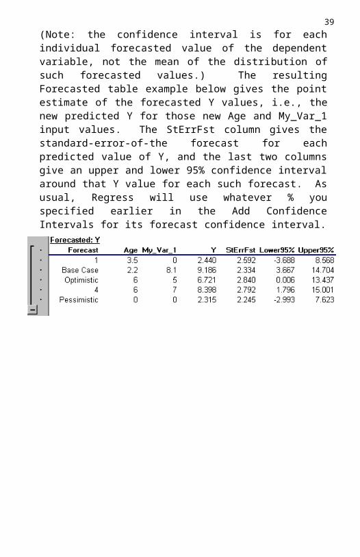
As shown below, Regress will add a “Forecasted” table to your regression results report containing the point prediction for each forecasting case (by plugging the given data values for the independent variables into the regression equation) and the Standard Error of the Forecast (“StErrFst”). If the Add Confidence Intervals option was checked in the Regression Results dialog, Regress will use the Standard Error of the Forecast to compute a confidence interval around that point forecast. (Note: the confidence interval is for each individual forecasted value of the dependent variable, not the mean of the distri-bution of such forecasted values.) The resulting Forecasted table example below gives the point estimate of the forecasted Y values, i.e., the new predicted Y for those new Age and My_Var_1 input values. The StErrFst column gives the standard-error-of-the forecast for each predicted value of Y, and the last two columns give an upper and lower 95% confidence interval around that Y value for each such forecast. As usual, Regress will use whatever % you specified earlier in the Add Confidence Intervals for its forecast confidence interval.

29

III Regress Tips and TechniquesScatter Plots

A handy option is to use Excel’s Chart Wizard to create XY scatterplots in your datasheet or your kept Regress reports for your model’s variables, taken two at a time. This allows you to see how the high or low correlations among your raw data appear visually, as shown below for two variables.

No. My_Var_1 Y Age1 2 5 22 3 5 03 9 8 54 1 2 15 5 4 06 2 6 27 3 5 08 8 12 19 2 5 310 0 1 0

0123456789

101112

0 1 2 3 4 5 6 7 8 9My_Var_1

Y

Non-Linear ModelsTo create non-linear regression models simply transform

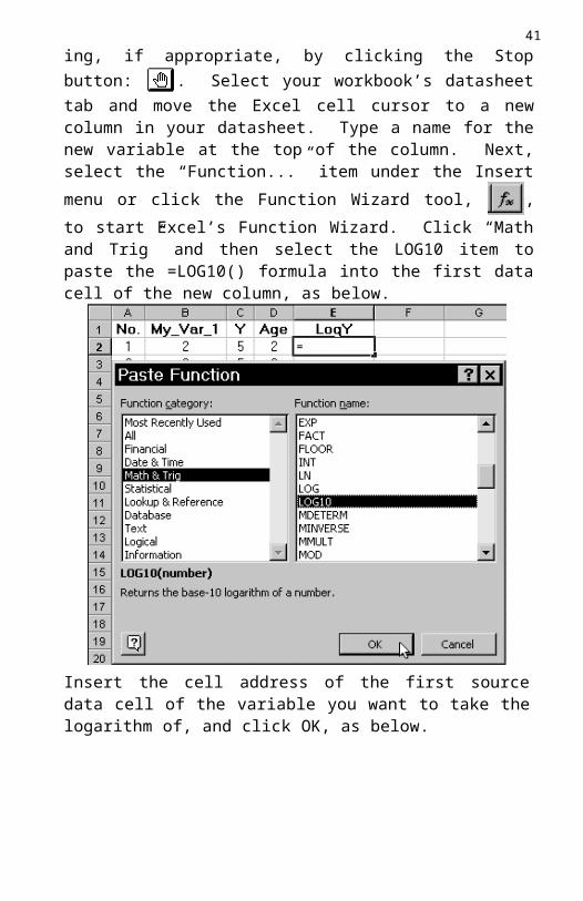
existing variables using standard Excel formulas or via Excel’s Function Wizard. For example, if you wish to create a new variable that is the Log transform of another variable, simply “Stop” Regress modeling, if appropriate, by clicking the Stop button: . Select your workbook’s datasheet tab and move the Excel cell cursor to a new column in your datasheet. Type a name for the new variable at the top of the column. Next, select the “Function...” item under the Insert menu or click the Function Wizard tool, , to start Excel’s Function Wizard. Click “Math and Trig” and then select the LOG10 item to

30paste the =LOG10() formula into the first data cell of the new column, as below.

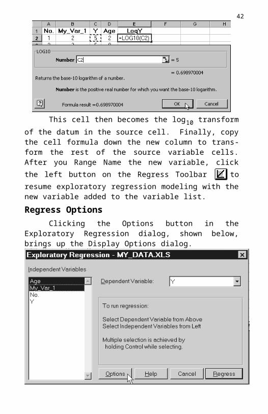
Insert the cell address of the first source data cell of the variable you want to take the logarithm of, and click OK, as below.

This cell then becomes the log10 transform of the datum in the source cell. Finally, copy the cell formula down the new column to transform the rest of the source variable cells. After you Range Name the new variable, click the left button on the Regress Toolbar to resume exploratory regression modeling with the new variable added to the variable list. Regress Options

Clicking the Options button in the Exploratory Regression

31dialog, shown below, brings up the Display Options dialog.

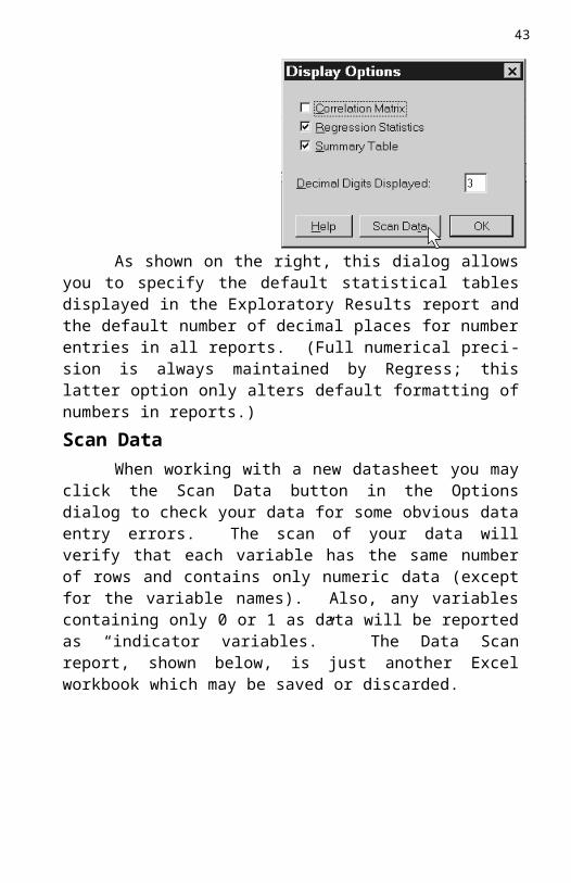
As shown on the right, this dialog allows you to specify the de-fault statistical tables displayed in the Exploratory Results report and the default number of decimal places for number entries in all reports. (Full numerical precision is always maintained by Regress; this latter option only alters default formatting of numbers in reports.)Scan Data

When working with a new datasheet you may click the Scan Data button in the Options dialog to check your data for some obvious data entry errors. The scan of your data will verify that each variable has the same number of rows and contains only numeric data (except for the variable names). Also, any variables containing only 0 or 1 as data will be reported as “indicator variables.” The Data Scan report, shown below, is just another Excel workbook which may be saved or discarded.

32

Bypassing Exploratory ResultsExploratory Results is designed to provide a quick evaluation

of your model which you can dismiss in favor of another model or keep in a permanent report. However, if you turn off all three tables in the Display Options dialog, Regress will bypass display of the Exploratory Results report and go directly to the Regression Results dialog. This saves a step or two if you know in advance you want to keep a report on a given model.Printing Regress Plots

Excel’s charting defaults include a gray shaded background behind all plots. This leads to pretty appearance of charts on color dis-play monitors. However, for monochrome LCD displays on laptops, and/or printing, this may cause an unacceptable loss of contrast as the colored charts are rendered into shades of gray, as illustrated below.

Histogram of Residuals

-4

-3.2

-2.4

-1.6

-0.8 0

0.8

1.6

2.4

3.2 40

0.20.40.60.8

11.21.41.61.8

2

Freq

uenc

y

-4

-3.2

-2.4

-1.6

-0.8 0

0.8

1.6

2.4

3.2 4

Residual Range

Histogram of Residuals

ResidualTheoretical

You may alter any of the shading, patterns, etc. defaults by means of the Picture toolbar enabled from the View\Toolbars menu. Using its controls you can increase the Brightness and/or Contrast to produce an image more acceptable to your display or printer, as shown below. You may also eliminate all colors by selecting the color button (to the left of the More Contrast button) and converting the plot to Grayscale or even Black & White.

33

Although less colorful, as shown below, these adjustments may lead to more acceptable black and white display or printing of Regress plots.

Histogram of Residuals

-4

-3.2

-2.4

-1.6

-0.8 0

0.8

1.6

2.4

3.2 40

0.20.40.60.8

11.21.41.61.8

2

Freq

uenc

y

-4

-3.2

-2.4

-1.6

-0.8 0

0.8

1.6

2.4

3.2 4

Residual Range

Histogram of Residuals

ResidualTheoretical

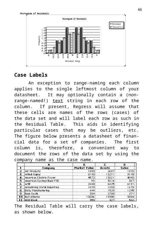
Case LabelsAn exception to range-naming each column applies to the

single leftmost column of your datasheet. It may optionally contain a (non-range-named!) text string in each row of the column. If present, Regress will assume that these cells are names of the rows (cases) of the data set and will label each row as such in the Residual Table. This aids in identifying particular cases that may be outliers, etc. The figure below presents a datasheet of financial data for a set of companies. The first column is, therefore, a convenient way to document the rows of the data set by using the company name as the case name.

34

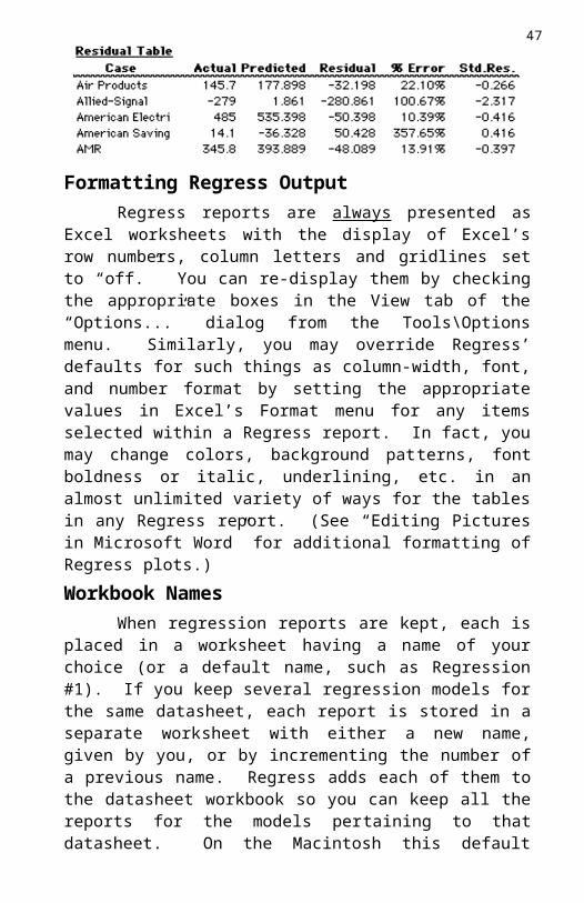
The Residual Table will carry the case labels, as shown below.

Formatting Regress OutputRegress reports are always presented as Excel worksheets with

the display of Excel’s row numbers, column letters and gridlines set to “off.” You can re-display them by checking the appropriate boxes in the View tab of the “Options...” dialog from the Tools\Options menu. Similarly, you may override Regress’ defaults for such things as column-width, font, and number format by setting the appropriate values in Excel’s Format menu for any items selected within a Regress report. In fact, you may change colors, background patterns, font boldness or italic, underlining, etc. in an almost unlimited variety of ways for the tables in any Regress report. (See “Editing Pictures in Microsoft Word” for additional formatting of Regress plots.)Workbook Names

When regression reports are kept, each is placed in a worksheet having a name of your choice (or a default name, such as Regression #1). If you keep several regression models for the same datasheet, each report is stored in a separate worksheet with either a new name, given by you, or by incrementing the number of a previous name. Regress adds each of them to the datasheet workbook so you can keep all the reports for the models pertaining to that datasheet. On the Macintosh this default workbook name is "Workbook1" and on Windows the default is “Book1.” You will have the opportunity to change this default workbook name when you Save your workbook to disk. Remember: You should save (backup) your workbook after every Regress report worksheet is added to it as protection against loss of results in case Excel runs out of memory.

35Recalculation

Be aware that in contrast to normal Excel spreadsheet use, in which formulas are “hot linked” to their data sources, changing the contents of one or more data cells within your datasheet after Regress has computed a regression model never results in automatic updating of the regression tables or charts produced from the original data. That is, no Excel hot links can be maintained between the original data and the regression results. If the contents of the original data must be changed then you must re-compute your regressions again to see the new results.Annotating Regress Tables and Charts in Excel

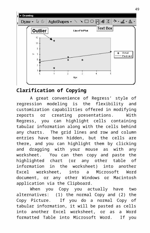
Additional annotation, such as Text Boxes and Arrows, can be added directly to any Regress table or chart by means of Excel’s Drawing Tools, as shown below for the text box containing “Outlier” and arrow. To enable these tools, select the Drawing item from Excel’s View\Toolbars menu.

Clarification of CopyingA great convenience of Regress’ style of regression modeling

is the flexibility and customization capabilities offered in modifying reports or creating presentations. With Regress, you can highlight cells containing tabular information along with the cells behind any charts. The grid lines and row and column entries have been hidden, but the cells are there, and you can highlight them by clicking and dragging with your mouse as with any worksheet. You can then copy and paste the highlighted chart (or any other table of information in the worksheet) into another Excel worksheet, into a Microsoft Word document, or any other Windows or Macintosh application via the

36Clipboard.

When you Copy you actually have two alternatives: (1) the normal Copy and (2) the Copy Picture. If you do a normal Copy of tabular information, it will be pasted as cells into another Excel worksheet, or as a Word formatted Table into Microsoft Word. If you Copy Picture then both tabular and graphical objects from Excel will be pasted as a single graphical picture object into Excel or Word. Since it is unlikely that you would want to edit cell results, the most convenient option is (2) Copy Picture. Once pasted as a graphic object into a Word document, you can use Microsoft Word's cropping and scaling features to adjust the size of the object conveniently, for example, to fit within the margins of your page.

Copy PictureTo perform a Copy Picture operation select the cells containing

the tables of interest and, if you wish, the cells behind any Regress chart. Next, hold down the Shift key while selecting the Edit menu. The Copy item in the Edit menu will change to “Copy Picture,” as shown on the right

Copy Picture -- Mac UsersAfter selecting Copy Picture, Macintosh users will be pre-

sented with the option to copy either “As Shown on Screen” or “As shown when printed.” Both work well for black and white Postscript-based laser printers, given the default colors used by Regress. Checking the “As shown when printed” option copies the object as it would appear in Print Preview, the preferred option so that colors are properly mapped into more legible patterns for almost all black and white printers.

37

Copy Picture --Windows UsersWindows users

will have to experiment with copying pictures into another application, such as Word. If you have a Postscript compatible laser printer, then you can behave like a Macintosh user. Otherwise, your choice is dependent on the resolution/features of your printer. Choosing “As shown when printed” option copies the object as it would appear in Print Preview and gives the best appearance while preserving any built-in fonts on your printer. However, if you re-size the picture either in Excel or Word before printing, then any text within the picture may not print neatly. This is because many inexpensive printers do not have scale-able fonts built-in, as do Postscript printers. So, the printing of text characters may not re-scale when you re-size the picture, thereby making the printed text appear jumbled because the fixed-sized characters do not scale with your re-sized picture. If you don’t have scale-able (Postscript or True Type) fonts on your printer, you should check “As shown on screen” and then choose Bitmap; see below. This makes the copied objects a single bitmap picture, including the text. Re-sizing the picture in Word then shrinks everything in the bit mapped graphic object together. Unfortunately, the bit mapped screen fonts will not print as sharply as using the printer’s build-in fonts, but the results should be adequate and you avoid mis-spaced characters in re-sized charts.

If you have a non-Postscript laser printer and opted for Copy Picture as a Bitmap, use the printer’s highest resolution for graphics printing. Normally, a printing resolution of 600 dots per inch or even 300 dots per inch will give quite adequate printing resolution for bit mapped objects, such as Regress plots and bit mapped table summaries. Note: be careful not to have too many bit mapped objects per printed page or your (non-Postscript) laser printer may run out of its internal page memory before the sheet is printed. Generally, 600 dots per inch is OK with default laser printer memory sizes, if you don't have more than about 30% of your page containing bit mapped objects. If you have problems printing graphic objects on laser

38printers, you may have insufficient laser printer memory for graphics printing. If you suspect the latter problem, try selecting a lower resolution to conserve the printer’s internal memory, or print fewer/smaller graphic objects per page. Pasting and Re-Sizing Pictures in Microsoft Word

Once you have Copied as Picture, switch to the other application, such as Word, and perform a Paste into your open document. It will be pasted as a graphic picture object. The default since Word97 is to paste a picture as a floating object. Unless you understand the nuances of positioning floating objects, you will want to paste the picture into a paragraph by itself to more easily center it, re-size it, etc. This is done by using Paste Special instead of Paste and un-checking the “Float over text” item. After pasting, if you wish to re-size the picture, click on the picture object. Sizing handles should appear as small boxes in the corners of the picture, as shown on the right.

Next, click on the lower right handle. While holding down the mouse button, drag in a northwesterly direction causing the picture to shrink. For most laser printers you can shrink an object down to 50% or smaller and still produce readable printing. Lower resolution printers may produce unreadable printed pictures, and thus, you may have to experiment with your particular printer. If you “Copy Picture” tabular information you may also perform this re-scaling, as well. Copy Picture Shortcut

An alternative and quicker way to copy just one chart from a Regress-produced worksheet in Excel is just to point to its border, click to reveal its (Excel) sizing handles (which also selects the object in Excel). This is shown on the right for the Histogram object. Next, Copy, switch to the Word document, and Paste/Paste Special. Now you can re-size, etc. in Word as discussed above.

39Note: If you select the cells behind a chart, as below, you must

Copy Picture or you will just get a copy of the empty cells behind the chart object when you Paste into a Word document.

Editing Pictures in Microsoft WordTo edit the components of pictures in Word you must first

Copy Picture from Excel, as before, except you must select “As shown on screen.” (Windows Excel users must also select the “Picture” option, as shown below, to produce a Windows Metafile object; a bit mapped object does not have any editable components within it.)

Switch to Word, and perform a Paste/Paste Special into your

open Word document. Your selection will be pasted as a graphic picture object. Next, right click the object and select Edit Picture

40(double click the object in Word 97 or Macintosh Word 98) to open Word’s Edit Picture window. Your picture object will be copied into it by Word and Word’s Drawing toolbar will be displayed to allow editing changes to be made.

In the figure below from Word, the Drawing toolbar was used (after ungrouping its components) to change and move the title of the line fit plot, change the regression line to a dotted line, to double the size and outline the outlier data point, and to boldface the X-axis title. Closing the Picture window pastes the revised object back into your original Word document. Review your Microsoft Word documentation for details on the editing of pictures, or consult Word’s Help files for additional information.

Copying and Pasting Outlined Information If some of Regress’ Tables are collapsed, then copying in-

formation from a Regress-produced worksheet can be a bit confusing. First, you need to understand the difference between Copy and Copy Picture, as explained above. Second, you need to be clear about how selections of worksheet areas are done by Excel in specifying what to copy.

Below is an example of a typical Regress report. It is a work-sheet, with standard worksheet rows and columns (the grid lines and row/column headers are set not to display by default -- you can display them via the View tab dialog by selecting the “Options...” item on the Tools menu.). Note that the Descriptive Statistics Table is collapsed.

41

Below, the cells of the top two tables have been selected by click/dragging. Note that the range of rows so selected includes the visible rows and the ones hidden by the collapsed outline.

If you Copy the selection and then Paste it into another Excel worksheet which has no outlining, you will get the expanded in-formation, as below, because all the rows you selected (hidden and unhidden) were copied. (Grid lines would also show, if the new worksheet has them set to display.)

However, depending on your version of Excel, pasting the information into Word will either show the hidden rows or it won’t. Recent versions of Excel (after Excel 97) will not paste the hidden rows. Note that pasting this information into Word, with or without hidden rows, will be formatted as a Word Table, each entry of which can be edited in Word.

Copying into a Word Table, as above, is thus available but rarely needed, since you will almost never want to edit those table entries in Word itself. The figure below shows the result of performing a Copy Picture with the previous selection, followed by a Paste/Paste Special into either an Excel worksheet or a Word document. Not surprisingly, it is pasted as a picture object of the information exactly as displayed. Most often this is what you will want to do.

42

Viewing the ClipboardOne way to make sense of copying from Excel is to open the

Clipboard window. For Macintosh this can be found as Show Clipboard on the Edit menu under Finder.

Windows has a separate Clipboard Viewer application. Click the Start button, and as below, select Accessories from the Programs menu, and launch the Clipboard Viewer application which produces a Clipboard window. This clipboard window can be positioned for convenient viewing on the Windows desktop before switching back to Excel.

Now when you select ranges of cells or objects and Copy, you can see what Excel is copying when it updates its Clipboard. However, even when viewing the Clipboard, different versions of Excel handle hidden rows of a collapsed outline differently, depending upon whether the Paste occurs within Excel or into another application, such as Word. You will need to experiment for your configuration to see how your versions of Excel copy any collapsed rows.Regress Comments

Regress further documents your work by placing the workbook name on the far right of the first line of every report. Also, an Excel comment is added to the dependent variable cell for documentation. As shown below, the comment documents the time and day the model

43was run, the computer (Macintosh or Windows) and OS version, the version of Excel (Excel 2000 is officially Excel version 9), and the workbook name and datasheet name. This information will pop up if you move the cursor over that cell. (“Show comment indicator” must be checked in the View tab of Excel’s Tools\Options… dialog to enable the pop up display.)

In addition, Regress will print the worksheet name at the top of every printed page.

44

IV Problems and Error MessagesResponse time and Memory Demands of Excel

Macintosh users please note: Excel on Macintosh uses only as much memory as allocated to it by the “Preferred Size” parameter of Macintosh Excel. The default size of this parameter produces a too small primary memory partition for Excel. A severe response time penalty is then caused by virtual memory swaps to disk when large worksheets or Add-Ins, such as Solver or Regress, are loaded into Excel’s too small memory partition. This occurs no matter how much actual free RAM is present. Therefore, Macintosh Excel users must increase Excel's default memory allocation by 1 or 2 megabytes or more as Excel’s “Preferred Size.” To change the default partition size for Macintosh Excel, quit Excel, open the folder containing the Excel application, and click the Excel application icon itself once to select it. Next, press Command+i to display the Macintosh System’s in-formation dialog for Excel, select Show Memory, and increase the “Preferred” memory size by 1 or 2 megabytes or more.Lesson: If Regress runs slow on a Macintosh, consider increasing Excel’s Preferred memory size.

A common problem, especially for large data sets, is the memory demands of Regress reports. It is very easy to become so engrossed during an exploratory Regress modeling session that you forget how much information you have kept in worksheet reports. During a single modeling session, it is not unusual to keep fifteen or more different regression models, each with a half-dozen scatter plots/Line Fit plots/Histograms, etc., all bundled into one workbook. From Excel’s viewpoint, however, you really have 15 or more worksheets open simultaneously (plus the temporary ones created by Regress at times) containing many tables and a total of 100 or more charts! Random access memory (RAM) demands can quickly become horrendous. Unfortunately, neither the Macintosh nor Windows operating systems manage RAM memory very well, and an Excel or system “crash” is possible when free memory gets very low. This is especially a problem in Windows 95/98 which uses small, fixed sized segments for its so-called User/GDI memory17. The segments’ memory contains information about Windows graphical objects and frequently is exhausted long before physical RAM or swap-disk memory is filled.

If you wait until you get an “Out of Memory” message from Excel, it may be too late to save your work because of insufficient free RAM (or System/GDI memory) to complete the Save operation itself, a very frustrating situation. So, always protect your work by saving your workbook to disk after every Regress report adds a worksheet to

17 Windows NT users do not have these memory allocation problems.

45your datasheet’s workbook.

A way to monitor memory use is to open the “About Microsoft Excel” dialog under the Apple menu (Macintosh) or under the Help menu (Windows). Macintosh users can examine the “Available Memory” to Excel entry in the dialog box. Windows 95/98 users must click the dialog’s “System Info...” button which produces a detailed status display of System’s Information, including the “USER” and “GDI” percentages. These are the primary indicators of any low memory condition. These statistics signal pending trouble in Windows if either falls below about 10%. If Windows User/GDI memory becomes low, you must increase it by closing unnecessary windows or workbooks within Excel or quitting or closing open windows in any other running Windows application.

If available memory becomes low during a Regress session, another alternative to free up memory is to click the rightmost Regress button, , if it is showing, to finish with the current model, and then save your workbook to disk. Next, select the “Move or Copy Sheet...” command from Excel’s Edit menu and copy your datasheet from the current workbook to a new workbook. Finally, close the original workbook (without a second save). Since the new workbook contains only your datasheet, available memory is increased allowing you to accumulate more “kept” Regress reports from further exploratory modeling. Later, after quitting and unloading Regress from memory by clicking its quit button, , you can consolidate related workbooks by opening each of them in turn and click/dragging the worksheet tabs of the kept report sheets from one workbook to the other.Lesson: If your get Excel’s “Out of Memory” message, increase Excel’s Preferred memory size (Macintosh) or reduce User/GDI mem-ory demands by closing unnecessary windows or other applications (Windows 95/98) or reduce the amount of memory devoted to holding the “kept” worksheet reports by saving the workbook to disk and opening a new workbook containing your datasheet but empty of previous Regress reports (both Macintosh and Windows).Multi-Collinearity Problems

The “multi-collinearity” error message from Regress is frequently confusing. Often, the root cause of this error is related to problems in the data or in specifying independent variables. For example, creating a new variable by transforming another variable will produce the multi-collinearity error message if both variables are used as independent variables and one is a linear function of the other. If, for example, you create a new variable by taking, say, the square root of another variable be sure to transform the variable by raising it to the .5 power instead of multiplying it by .5.

46Lesson: Double check your datasheet results whenever you use a formula or function to transform one variable to create a new one to assure that the two are not linearly related. A quick check of this can be done by looking at the correlation between the two variables, which will be 1.000 if they are linearly related.

Another source of this message occurs if the data variables are range named as rows instead of as columns. Regress expects its datasheet to have its variables define range named columns, not range named rows. If the variables are defined as referring to rows, Regress will produce the multicollinearity error message.Lesson: Double check your datasheet to be sure the variables define column variables. Use the Regress Scan Data feature, described on page 30, to scan your data to verify that the range names for each variable refer to a column.

Surprisingly, it is possible to get the multi-collinearity error message even if there is only one independent variable in your model, i.e., a simple linear regression. If the one independent variable chosen happens to have no variation in its values, then in effect, that one variable is collinear with the internal variable created to compute the regression model’s intercept coefficient. Lesson: If you choose a variable for incorporation into a regression model, either as a dependent or an independent variable, there must be some variation in the values down the column for that variable. If it is a constant down the column, then no calculation can be performed to compute that variable’s regression coefficient.

For multiple regression models, a common mistake is to assume that the only way the multicollinearity message could occur is if the correlation between two independent variables is one. Indeed, that is the most frequent source of this difficulty. However, multicollinearity can occur if there is any perfect dependency among any subset of the independent variables in a model taken as a group, not just two at a time. The most likely source of this group-of-variables occurrence is with collections of related indicator variables. For example, imagine that each row (case) in your data set concerns an employee who works in one of four possible company departments. You set up four indicator variable columns for the four departments and place a 1 in the proper department column for that employee to signal his department membership. Hence, each row in your data matrix has a 1 in one of the four columns to signal which department that person belongs to with the remaining three cells in the row containing zeros. However, if you create a model specifying all four department indicator variables as independent variables, you will get the multicollinearity error message. Why is this? Because for each row in your datasheet, if you know the values for three of the depart-

47ment cell entries, you can unambiguously deduce what the fourth one must be. Hence, the four department variables as a group are not inde-pendent of each other, thereby producing the multicollinearity error message. How do you solve this problem? Select one of the 0/1 de-partment variables as your “base case” and leave it out of every regression in which you specify the other three department variables. This breaks the dependency and allows a straightforward interpretation: the coefficient on each of the included department variables is interpreted with respect to the left-out department base case.

Another related problem occurs when a group of variables consist of rank numbers. Like the department example above, if say, five columns are devoted to representing rank numbers between one and five, then if you know four of the five rank numbers, you can unambiguously deduce what the fifth one is, thereby inducing multicollinearity again. Lesson: If you get the multicollinearity error message and the correla-tion matrix does not identify perfect correlation between two of the independent variables, consider whether you have induced dependence among groups of related independent variables. “Text in Data” Error Message and Missing Data

The “Text in Data” message occurs whenever Regress encounters illegal data in a variable. In particular, you cannot ever have any text characters in your datasheet cells: they must always contain numeric data, including, of course, the characters - and decimal point, or formulas that produce numeric results.

One Regress user kept getting this error message but remained convinced that he had no text in his data. Further inspection revealed that missing data had been encoded as a single “.” by the organization from which he got the data. The “.” in a cell is almost invisible on a typical display screen, and so, was not seen. Lesson: Use the Regress Scan feature to scan your data to assure there are no text characters in any datasheet variables’ cells.

Missing data appears to be a troublesome source of difficulty in general. One user kept getting “insufficient number of cases” error messages because he assumed, as is common in spreadsheet usage, that every empty cell in Excel would be automatically read as a zero. To save typing, therefore, for his indicator variable entries, he typed only the ones, leaving the other cells empty to signify a zero. As a result, however, Regress marked most of his cases as “missing” and ignored almost all his data in regression modeling. In order to handle missing data, Regress makes a major distinction between an empty cell (which always signals missing data) and a cell containing a zero. Lesson: Enter all data items explicitly, including zeroes.

48Another user encoded missing data by typing a space in the

cell. Obviously, the appearance of the resulting worksheet screen image of the data suggests the cell to be “empty.” Unfortunately, the cell is not empty and contains the “space” text character. Since the cell is not actually empty, the Regress missing value routine is not evoked and so, the cell containing the space character is passed on to the computational routines with predictable results of the “Text in Data” error. Lesson: Be sure that there is no text of any kind in any data cell, including any space characters which may make it appear as if the cell is empty. The way to force a cell to be empty is to use the “Clear” command under the Edit menu.

Tip 1: Use the “Scan Data” option available under Regress’ Options button in the Exploratory Regression dialog (where you first specify your dependent and independent variables). It will catch any text in your datasheet associated with any range-named variable.

Tip 2: For an easy way to eliminate any (known) text charac-ters from all your data cells, select the “Replace...” item from Excel’s Edit menu to search for those character(s) and use an empty “Replace With” entry in the dialog box.Problems with Range Names

The “That is not a valid datasheet.” error message usually means that you forgot to Range-Name the variables in your datasheet, and hence, Regress cannot find any variables to work with.

A similar problem is caused by being too casual in high-lighting data when selecting the “Name Create” item in the Insert menu. As a result, over time, the range names defining data columns end up being of different lengths. Regress will respond by marking the shorter columns as having missing values at their ends, producing confusing “Missing Cases” entries in the Regression Summary Table.Lesson: After any modifications to your datasheet, “Data Scan” your datasheet for valid range name definitions and review them carefully.

Excel treats all range names for every worksheet in a workbook as global. Therefore, Regress will always list all the range names associated with a given workbook not just the active worksheet. Although very flexible in that it allows data variables to be scattered across several worksheets in a workbook, this can lead to confusion if you have multiple worksheets in the workbook, each with their own collection of range names that are unrelated to your data. Lesson: To avoid confusion in selecting variables in Regress, range name only the variables in your datasheet and dedicate the workbook to containing only your datasheet and collections of related Regress report sheets.

49