1

Regional Ocean Modeling System (ROMS) Hernan G. Arango1, John L. Wilkin1, and Andrew M. Moore2

1 Department of Marine and Coastal Sciences, Rutgers, The State University of New Jersey, 71 Dudley Road, New Brunswick, NJ 08901-8521, arango@marine.rutgers.edu, jwilkin@rutgers.edu. 2 Department of Ocean Sciences, University of California Santa Cruz, 1156 High Street, Santa Cruz, CA 95064, ammore@ucsc.edu Web Links: www.myroms.org, www.myroms.org/wiki/Documentation_Portal

Introduction ROMS is an open-source, mature numerical framework used by both the scientific and operational

communities to study ocean dynamics over a wide range of spatial (coastal to basin) and temporal (days to seasons, years to decades) scales. It is unique in that is the only community framework including the adjoint-based analysis and prediction tools that are available in Numerical Weather Prediction (NWP), like 4-dimensional variational data assimilation (4D-Var), ensemble prediction, observations sensitivity and impact, adaptive sampling, and circulation stability and sensitivity analysis. ROMS is freely distributed (http://www.myroms.org) to the Earth’s modeling community and has thousands of users worldwide.

The development and continuous evolution of ROMS has been performed primarily with Office of Naval Research funding to Arango, Moore and others over the last few years. The major strengths of ROMS are its continuous evolution and improvement, its comprehensive algorithms and options to explore diverse ocean modeling applications, and its very vibrant and active user community. The success of ROMS can be measured in terms of the thousands of users worldwide, the hundreds of peer-reviewed articles in scientific journals and books, and the research work of numerous Ph.D. students and post-doctoral fellows. ROMS is been used to train the next generation of ocean modeling scientists.

Currently, ROMS can be used in basin and global scale applications and is no longer limited to regional scale. However, running high-resolution basin or global scale applications to resolve important topographic features and smaller-scale phenomena is prohibitively demanding on computational resources. An efficient strategy is to use grid nesting in areas of the coarser grid where smaller scale features need to be better resolved. Technical Description

1. Dynamical Kernel

ROMS is a three-dimensional, free-surface, terrain-following ocean model that solves the Reynolds-averaged Navier-Stokes equations using the hydrostatic vertical momentum balance and Boussinesq approximation (Haidvogel et al. 2000; Shchepetkin and McWilliams, 2005). The governing dynamical equations are discretized on a vertical coordinate that depends on the local water depth. The horizontal coordinates are orthogonal and curvilinear allowing Cartesian, spherical, and polar spatial discretization on an Arakawa C-grid. Its dynamical kernel includes accurate and efficient algorithms for time-stepping, advection, pressure gradient (Shchepetkin and McWilliams 2003, 2005), several subgridscale parameterizations (Durski et al., 2004; Warner et al., 2005) to represent small-

2

scale turbulent processes at the dissipation level, and various bottom boundary layer formulations to determine the stress exerted on the flow by the bottom.

The momentum equations are solved using a split-explicit time-stepping scheme that requires special treatment and coupling between barotropic (fast) and baroclinic (slow) modes. A finite number of barotropic time steps, within each baroclinic time step, are carried out to evolve the free-surface and vertically integrated momentum equations. A cosine-shape time filter, centered at the new time level, is used for the averaging of the barotropic fields (Shchepetkin and McWilliams, 2005). In addition, the separated time stepping is constrained to exactly maintain both volume conservation and constancy preservation properties, which are needed for the tracer equations (Shchepetkin and McWilliams, 2005). By default, the 2D and 3D equations are time-discretized using a third-order predictor (Leap-frog) and corrector (Adams-Molton) scheme, which is very robust and stable. The enhanced stability of the scheme allows larger time steps, by a factor of about four, which more than offsets the increased cost of the predictor-corrector algorithm.

2. Numerical Kernel

ROMS is a very modern and modular code written on F90/F95. It uses C-preprocessing to activate the various physical and numerical options. The parallel framework is coarse-grained with both shared-memory (OpenMP) and distributed-memory (MPI) paradigms coexisting in the same code. Because of its construction, the parallelization of the adjoint is only available for MPI. Several coding standards have been established to facilitate model readability, maintenance, and portability. All the state model variables are dynamically allocated and passed as arguments to the computational routines via dereferenced pointer structures. All private arrays are automatic; their size is determined when the procedure is entered. This code structure facilitates computations over nested grids.

The coupling between multi-models can be done directly or indirectly. In direct coupling, the considered models are run simultaneously and data exchange is done at predetermined synchronization points using the Model Coupling toolkit (MCT) communications library (Larson et al., 2005). This approach has been used successfully to couple ROMS with atmospheric and wave models (Warner et al., 2008b). The coupling is volumetric and conservation properties are preserved. The exchange of data between models can be one-way or two-way. Direct coupling is also possible using the Earth System Modeling Framework (ESMF, version 7.0) library. Work is underway to implement the Unified Operational Prediction Capability (NUOPC) ESMF layer to enhance interoperability with other modeling systems. Contrarily, indirect coupling is achieved by saving into NetCDF files the lateral boundary conditions for free-surface, momentum, and active and passive tracers and surface forcing at regular time intervals. The coupling data is read from input NetCDF files and time interpolated between available snapshots.

3. Sub-Models There are several biogeochemical models available in ROMS. In order of increasing ecological

complexity these include three NPZD-type models (Franks et al., 1986; Powell et al., 2006; Fiechter et al., 2009), a nitrogen-based ecosystem model (Fennel et al., 2006, 2008), a Nemuro-type lower level ecosystem model (Kishi et al., 2007), and a bio-optical model (Bissett et al., 1999).

ROMS includes a sediment-transport model with an unlimited number of user-defined cohesive (mud) and non-cohesive (sand) sediment classes (Warner et al., 2008a). Each class has attributes of grain diameter, density, settling velocity, critical stress threshold for erosion, and erodibility constant. A multi-level bed framework tracks the distribution of every size class in each layer and stores bulk properties including layer thickness, porosity, and mass, allowing the computation of bed morphology

3

and stratigraphy. Also tracked are bed-surface properties like active-layer thickness, ripple geometry, and bed roughness. Bedload transport is calculated for mobile sediment classes in the top layer.

ROMS offers an air-sea interaction boundary layer, which is based on the bulk parameterization of Fairall et al. (2003). It was adapted from the Coupled Ocean-Atmosphere Response Experiment (COARE) algorithm for the computation of surface fluxes of momentum, sensible heat, and latent heat. This boundary is used for one- or two-way coupling with atmospheric models.

4. Adjoint-based Algorithms and Data Assimilation The ROMS tangent linear (TLM) and adjoint (ADM) models were hand-coded (Moore et al.,

2004) from the discrete code using the recipes of Giering and Kaminski (1998). The discrete adjoint is exact and is defined relative to the inner product that defines the L2-norm. There is an additional tangent linear model (RPM) that computes a finite amplitude linear estimate of the total state of the system as opposed to perturbations about some existing solution of the nonlinear model (NLM). The RPM is used for representer-based data assimilation.

Several adjoint-based algorithms exist to explore the factors that limit the predictability of the circulation in regional applications for a variety of dynamical regimes (Moore et al., 2004). These algorithms use the ideas of Generalized Stability Analysis (GSA) in order to identify the most unstable directions of state-space in which errors and uncertainties are likely to grow. The resulting singular vectors can be used to construct ensembles of forecasts by perturbing initial and boundary conditions (optimal perturbations) and/or perturbing surface forcing (stochastic optimals). Perturbing the system along the most unstable directions to the state-space yields information about the first (ensemble mean) and second (ensemble spread) moments of the probability density function. Given an appropriate forecast skill measure, the circulation is predictable if low spread and unpredictable if large spread.

ROMS uniquely supports three different 4D-Var data assimilation methodologies (Moore et al., 2011a, b): a primal form of the incremental strong constraint 4D-Var (I4D-Var), a strong/weak constraint dual form of 4D-Var based on the Physical-space Statistical Analysis System (4D-PSAS), and a strong/weak constraint dual form of 4D-Var based on the indirect representer method (R4D-Var). In the dual formulations, the search for the best ocean circulation estimate is in the subspace spanned only by the observations, as opposed to the full space spanned by the model as in the primal formulation. Although the primal and dual formulations yield identical estimates of the ocean circulation for the same a priori assumptions, there are practical advantages and disadvantages to both approaches (Moore et al., 2011a, b, c). These algorithms have been used in several regional applications (Broquet et al., 2009; Powell et al., 2008, 2009; Di Lorenzo et al., 2007; Muccino et al., 2008). Additional algorithms exists (Moore et al., 2011b, c) to (i) estimate the posterior error or confidence in the resulting circulation estimates; (ii) quantify the sensitivity of the observations to the R4D-Var and 4D-PSAS data assimilation systems, which may be used for observation system design and monitoring; and (iii) quantify the impact of each observation on the forecast analysis increment for R4D-Var and 4D-PSAS, allowing us to identify which observations have the greater impact in the circulation estimate. Some of these algorithms require the adjoint of the 4D-Var data assimilation system, denoted as (4D-Var)T. Currently, (4D-Var)T is only available for the dual formulation algorithms (4D-PSAS and R4D-Var) because the adjoint of the Lanczos-based, conjugate gradient algorithm used in the minimization is much simpler. This capability is challenging in I4D-Var due to the complexity of the I/O intensive, Lanczos-based, conjugate gradient and preconditioning algorithms that are used when the minimization is carried out in model space. To our knowledge, ROMS is the only open-source, ocean community-modeling framework supporting all these variational data assimilation methods and other sophisticated adjoint-based algorithms.

4

The observation impact algorithm can be used to quantify the contribution of each observation during a 4D-Var analysis to a specified aspect (scalar function, say I) of the ocean circulation (Langland and Baker, 2004; Gelaro and Zhu, 2009; Trémolet, 2008; Moore et al., 2011c). That is, it identifies the part of the model space that controls I and that is activated by the observations. It yields the actual contribution of each observation to the circulation increment.

The observation sensitivity is based on (4D-Var)T and quantifies the change that would result in the circulation estimate as result of changes in the observations or observation array (Trémolet, 2008; Moore et al., 2011c). It is a very useful tool for efficient generation of observation system experiments (OSEs), observation array design, and adaptive sampling. It can also be used to predict the changes that will occur in I in the event of a platform failure or a change in the observation array (Moore et al., 2011c).

The array modes of the stabilized representer matrix can be used to determine the most stable component of the circulation with respect to changes in the innovation vector (Bennett, 1985; Moore et al., 2011c). The array modes are independent of the observation values and depend only on the observation locations, the prior covariances, and prior circulation.

An adjoint sensitivity algorithm is available in ROMS for efficiently exploring the linear time dependent response of the circulation fields to variations in all physical and biological attributes of the system (Moore et al., 2009). Similarly, an optimal observation (adaptive sampling) driver is available to help design observational networks and improve ocean prediction. This driver is an enhanced adjoint sensitivity algorithm, but the tangent linear model is used to propagate the analysis and determine the optimal location of the observations.

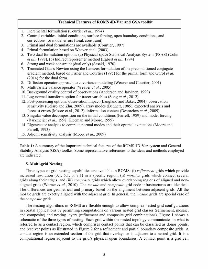
A summary of the important technical features of ROMS 4D-Var system and the GSA toolkit is shown in Table 1. Some representative references to the ideas and methods employed are indicated.

Additionally, Ensemble Kalman Filter (EnKF) data assimilation is possible in ROMS using the Data Assimilation Research Testbed (DART; Anderson et al., 2009; Anderson, 2009) developed and maintained at the National Center for Atmospheric Research (NCAR). Ensemble filters (Evensen, 1994; Houtekamer and Mitchell, 1998; Burgers et al., 1998) are Monte Carlo approaches to the data assimilation problem that are an alternative to variational methods. An ensemble of model forecasts is produced by a model and the sample statistics are used to incorporate observations as they become available. No adjoints, linear tangents or prior estimates of error covariance between the observations and state components are required.

The DART system can process ROMS output observation NetCDF files that map the nonlinear model state to the expected observation value in space and time. This is achieved by running the ROMS nonlinear model with the VERIFICATION option activated and providing the input observation data, which is the same input observation NetCDF file used in 4D-Var. The fact that both 4D-Var and EnKF are available in ROMS provides the user communities with the opportunity to explore the relative merits of each approach to data assimilation. We foresee the development of a hybrid EnKF/4D-Var system that will capitalize on the merits of both ensemble and variational approaches. That is, the flow-dependent prior error covariances of EnKF and the adjoint-based dynamical interpolation inherent in 4D-Var.

5

Technical Features of ROMS 4D-Var and GSA toolkit

1. Incremental formulation (Courtier et al., 1994) 2. Control variables: initial conditions, surface forcing, open boundary conditions, and

corrections for model errors (weak constraint) 3. Primal and dual formulations are available (Courtier, 1997) 4. Primal formulation based on Weaver et al. (2003) 5. Two dual formulation options: (a) Physical-space Statistical Analysis System (PSAS) (Cohn

et al., 1998), (b) Indirect representer method (Egbert et al., 1994) 6. Strong and weak constraint (dual only) (Sasaki, 1970) 7. Truncated Gauss-Newton using the Lanczos formulation of the preconditioned conjugate

gradient method, based on Fisher and Courtier (1995) for the primal form and Gürol et al. (2014) for the dual form.

8. Diffusion operator approach to covariance modeling (Weaver and Courtier, 2001) 9. Multivariate balance operator (Weaver et al., 2005) 10. Background quality control of observations (Anderson and Järvinen, 1999) 11. Log-normal transform option for tracer variables (Song et al., 2012) 12. Post-processing options: observation impact (Langland and Baker, 2004), observation

sensitivity (Gelaro and Zhu, 2009), array modes (Bennett, 1985), expected analysis and forecast errors (Moore et al., 2012), information content (Desroziers et al., 2009).

13. Singular value decomposition on the initial conditions (Farrell, 1989) and model forcing (Barkmeijer et al., 1998; Kleeman and Moore, 1999).

14. Eigenvector analysis to compute normal modes and their optimal excitations (Moore and Farrell, 1993)

15. Adjoint sensitivity analysis (Moore et al., 2009)

Table 1: A summary of the important technical features of the ROMS 4D-Var system and General Stability Analysis (GSA) toolkit. Some representative references to the ideas and methods employed are indicated.

5. Multi-grid Nesting

Three types of grid nesting capabilities are available in ROMS: (i) refinement grids which provide increased resolution (3:1, 5:1, or 7:1) in a specific region; (ii) mosaics grids which connect several grids along their edges, and (iii) composite grids which allow overlapping regions of aligned and non-aligned grids (Warner et al., 2010). The mosaic and composite grid code infrastructures are identical. The differences are geometrical and primary based on the alignment between adjacent grids. All the mosaic grids are exactly aligned with the adjacent grid. In general, the mosaic grids are special case of the composite grids.

The nesting algorithms in ROMS are flexible enough to allow complex nested grid configurations in coastal applications by permitting computations on various nested grid classes (refinement, mosaic, and composite) and nesting layers (refinement and composite grid combinations). Figure 1 shows a schematic of the three types of nesting. Each grid within the nested topology communicates in what is referred to as a contact region, which comprises contact points that can be classified as donor points, and receiver points as illustrated in Figure 2 for a refinement and partial boundary composite grids. A contact region is an extended section of the grid that overlays or is adjacent to a nested grid. It is a computational region adjacent to the grid’s physical open boundaries. A contact point is a grid cell

6

inside the contact region. The contact points are located according to the staggered Arakawa C-grid horizontal positions. The strategy is to compute the full horizontal operator at the contact points between nested grids instead of specifying open boundary conditions and/or fluxes.

Figure 1: Schematic examples of (a) a mosaic grid, (b) a composite grid, and (c) a refinement grid in ROMS.

Figure 2: An illustration of the contact regions (shown in purple) and contact points for composite (grid 2) and refinement (grid 3) connected to coarser grid 1. The contact regions for grid 1 (donor) to grids 2 and 3 (receivers) are shown in (a) whereas the contact regions for grids 2 and 3 (donors) to grid 1 (receiver) is shown in (b). The contact region between grids 3 and 1 in (b) is used in the fine to coarse averaging step. Notice the duality of a ROMS nested grid: data donor in one contact region and data receiver in its conjugate region. The exchange of information is always two-way.

a b c

a b

1 1

2 2

3 3

7

ROMS nesting numerical stencils process enough contact points in the contact region to fully compute the high-order spatial operators (advection, diffusion/viscosity, pressure gradient) adjacent to the nested finer grid boundary. Other models only specify the boundary value and an estimate of the flux through the boundary for a particular state variable.

The grid refinement strategy for one-way and two-way nesting has been studied extensively in both atmosphere and ocean models. Penven et al. (2006) evaluates one-way nesting in ROMS (UCLA F77-version) using the AGRIF (Blayo and Debreu, 1999) embedding package. Rutgers’s version of ROMS is already written in F90 and has pointer structures for the dynamical allocation of model arrays for all nested grids, so the AGRIF library is not needed and redundant. Our nesting strategy is unique and robust. The data exchange between nested grids is two-way by default, as illustrated in Figure 1. We have very successful applications in various dynamically complex regions around the world. For example, Figure 3 shows downscaling refined applications in US East Coast centered in North Carolina (Warner et al., 2010) and the Mid-Atlantic Bight (Figure 4). The refined grid solutions are overlaid on top of the coarser grid solution. The exchange of information between the grids is seamless and very stable. This is a very difficult dynamical regime in which to put nested grids due the vicinity and variability of the Gulf Stream.

The concept of mosaic grids was developed at GFDL by Balaji et al. (2006) for climate research. The mosaic grids, of equal or different resolutions, connect two grids along their common boundary edge. The quantities transferred between them are interpolated onto the exchange cells, which overlap each grid in order to compute the advective/diffusive fluxes between them. An example of mosaic grid in ROMS is shown in Warner et al. (2010) for an idealized dog-bone test. It is a simple application used to study the gravity wave advection between two basins connected with a narrow channel, resulting in a dog-bone shaped grid. The approach is to solve the system as a single grid or as two grids (mosaics) connected at the middle and having one common boundary edge. Identical results are obtained, at all times, when comparing the single grid against the two mosaic grids solutions (Warner et al., 2010). This is a rigorous test to check if this nested approach is coded correctly.

The composite grid nesting approach is similar to the mosaic grids but the grids overlap each other by several grid cells, as illustrated in Figure 5 for the Hudson River System application (Warner et al., 2010). Three independent grids representing the Hudson River, New York Harbor, and East River are connected and solved simultaneously to accurately simulate the complex estuarine tidally-forced circulation. The sediment concentration (kg/m3) and sediment bed thickness (m) are affected by the spring/neap tidal amplitude variability in the estuary.

Extensive information for the ROMS nested grids Super-Classes and Sub-Classes topologies are provided in WikiROMS (www.myroms.org/wiki/Nested_Grids). Notice that the contact regions and contact points are processed outside of ROMS and read in from an input connectivity NetCDF file. Currently, the connectivity file is generated and processed with several Matlab scripts described in WikiROMS (www.myroms.org/wiki/Matlab_Processing_Scripts).

8

Figure 3: Refined nested grid application for the North Carolina outer banks application (Warner et al., 2010): (a) diagram showing four grids with decreasing averaged horizontal resolution 5 km, 1 km, 200 m, and 40m, and (b) snapshot of sea surface temperature (oC, color map) and surface currents (m/s, arrows) for the 5km grid and 1km grid (inset).

1000 m

5000 m

200 m 40 m

SST (°C) and Surface Currents (m/s)

9

Figure 4: Free surface (m) for two-way nested applications in the Mid-Atlantic Bight: (a) two grids, DOPPIO (~7 km) and Hudson Canyon (~2.3 km); (b) three grids, DOPPIO, Hudson Canyon, and Pioneer Data Array (~1 km). The snapshot is for 15 May 2014, 135 days after initialization.

10

Figure 5: Hudson River modeling system (Warner et al., 2010): (a) composite grids for Hudson River estuary, Hudson River harbor and East River, (b) sediment concentration (kg/m3), and (c) sediment bed thickness (m).

Community Outreach

The user community and outreach is a very important component of ROMS development and evolution. The community outreach is done in the ROMS forum (www.myroms.org/forum) and workshops. We have been independently organizing annual workshops since 2004. Several very successful workshops were held at CNR-ISMAR (Venice, 2004), Scripps Institute of Oceanography (La Jolla, 2005), and University of Alcala de Henares (Spain, 2006), University of California at Los Angeles (Oct 1-5, 2007); Jean Kuntzmann laboratory, Saint Martin d'Heres Campus, Grenoble, France (Oct 6-8, 2008); Sydney Institute of Marine Science, Sydney, Australia (Mar 31 – Apr 2, 2009), University of Hawaii at Manoa, Honolulu, Hawaii (April 5-8, 2010); Windsor Atlântica Hotel, Petrópolis Conference Room, Rio de Janeiro, Brazil (Oct 22-25, 2012), and Island Hotel Istra, Island of St. Andrew's, Rovinj, Croatia (May 26-29, 2014). The next ROMS Asia-Pacific Workshop will be held Institute for Marine and Antarctic Studies, Hobart Waterfront, Tasmania, Australia on Oct 17-21, 2016. We held a Data Assimilation Workshop at the University of California Santa Cruz, Santa Cruz, CA, on Jul 12-16, 2010. This was a one week workshop that included lectures on 4D-Var data assimilation methodology and algorithms, practical 4D-Var tutorials using the US West Coast coarse grid application, observation processing, 4D-Var observation impact and sensitivity, and error covariance modeling. The next Workshop will be held in the summer of 2017 at NCEP, College Park, MD.

a. b. c.

11

Current and Future Developments ROMS is continuously changing and improving. Current and future areas of development are as follows:

• Fully coupled ROMS and COAMPS dynamics via ESMF and NUOPC. Fully coupled ROMS and COAMPS data assimilation (EnKF and 4D-Var).

• 4D-Var data assimilation within nested grids. Several strategies are being examined for 4D-Var data assimilation in either one-way or two-way nested grids.

• Hybrid, heterogeneous one-way nesting with a large-scale model. The large-scale model can be a ROMS application or any other model application. The exchange information between models at the regional ROMS open boundary conditions (hybrid contact points; orange region in Figure 6) is either concurrent or non-concurrent. The ESMF or MCT library is used for the concurrent exchange of information since all the nested models are running at the same time. In non-concurrent communications, the exchange of information is through NetCDF file(s) that have the appropriate data at the ROMS hybrid contact points, which is generated by the large-scale model or from its solution. Such boundary data is usually time interpolated between snapshots inside of ROMS. This new type of open boundary conditions is robust because ROMS computes the full high-order spatial operators (advection, diffusion/viscosity, pressure gradient) at the hybrid contact area. This is similar to the nested approach in various ROMS nested grids (see Figure 2).

• Sea Ice coupling to CICE via ESMF/NUOPC. Update ROMS Sea Ice model, then write its tangent linear and adjoint model for sea ice 4D-Var data assimilation and adjoint sensitivities.

12

Figure 6: Schematic of hybrid, heterogeneous nested grids and contact points. Blue region is central ROMS downscaled grid for a typical coastal application. Gray represents the coastline. Red shows further two-way nested or composite ROMS grids. Purple shows contact regions in which data is exchanged between grids to complete numeric stencil. Orange is the hybrid contact region where information is passed from the prototype large-scale model to ROMS.

13

References Andersson, E. and H. Järvinen, 1999: Variational quality control, Quart. J. Roy. Meteorol. Soc., 125,

697-722.

Anderson, J.L., 2009: Spatially and temporally varying adaptive covariance inflation for ensemble filters, Tellus, 61, 72-83.

Anderson, J.L., T.J. Hoar, K. Raeder, H. Liu, N. Collins, R. Torn, and A. Arellano, 2009: The data assimilation research test bed: A community facility, Bull. Am. Met. Soc., 90, 1283-1296.

Balaji, V., J. Anderson, I. Held, M. Winton, J. Durachta, S. Malyshev, and R.J. Stouffer, 2006: The Exchange Grid: a mechanism for data exchange between Earth System components on independent grids. Parallel Computational Fluid Dynamics: Theory and Applications, Proceedings of the 2005 International Conference on Parallel Computational Fluid Dynamics, May 24-27, College Park, MD, USA, A. Deane, G. Brenner, A. Ecer, D. Emerson, J. McDonough, J. Periaux, N. Satofuka, , and D. Tromeur-Dervout, eds., Elsevier.

Barkmeijer, J., M. van Gijzen and F. Bouttier, 1998: Singular vectors and estimates of the analysis-error covariance matrix, Quart. J. Roy. Meteorol. Soc., 124, 1695-1713.

Bennett, A.F., 1985: Array design by inverse methods, Prog. Oceanog., 15, 129-156. Blayo, E. and L. Debreu, 1999: Adaptive mesh refinement for finite-difference ocean models: first

experiments, J. Phys. Oceanogr., 29, 1239-1250. Bissett, W.P., K.L. Carder, J.J. Walsh, D.A. Dieterle, 1999: Carbon cycling in the upper water of the

Sargasso Sea: II. Numerical simulation of apparent and inherent optical properties, Deep-Sea Res., 46, 271-317.

Broquet, G., C.A. Edwards, A.M. Moore, B.S. Powell, M. Veneziani, and J.D. Doyle, 2009: Application of 4D-Variational data assimilation to the California Current System, Dyn. Atmos. Oceans, 48, 69-92, doi:10.1016/j.dynatmoce.2009.03.001.

Burgers, G., van Leeuwen, P.J. and G. Evensen, 1998: Analysis Scheme in Ensemble Kalman Filter, Mon. Wea. Rev., 126, 1719-1724.

Cohn, S., A. D. Silva, J. Guo, M. Sienkiewicz, and D. Lamich, 1998: Assessing the effects of data selection with the DAO physical-space statistical analysis system, Mon. Wea. Rev., 126, 2913–2926.

Courtier, P., 1997: Dual formulation of four-dimensional variational assimilation, Quart. J. Roy. Meteorol. Soc., 123, 2449–2461.

Courtier, P., J.-N. Thépaut, A. Hollingsworth, A., 1994: A strategy for operational implementation of 4D-Var using an incremental approach, Quart. J. Roy. Meteorol. Soc., 120, 1367–1388.

Desroziers, G., L. Berre, V. Chabot, and B. Chapnik, 2009: A posteriori diagnostics in an ensemble of perturbed analyses, Mon. Weather Rev., 137, 3420–3436.

Di Lorenzo, E., A.M. Moore, H.G. Arango, B.D. Cornuelle, A.J. Miller, B. Powell, B.S. Chua, and A.F. Bennett, 2007: Weak and Strong Constraint Data Assimilation in the inverse Regional Ocean Modeling System (ROMS): development and applications for a baroclinic costal upwelling system. Ocean Model., 16, 160-187.

14

Durski, S.M., S.M. Glenn, and D.B. Haidvogel, 2004: Vertical mixing schemes in the coastal ocean: Comparison of the level 2.5 Mellor-Yamada scheme with an enhanced version of the K profile parameterization, J. Geophys. Res., 109, C01015, doi:10.1029/2002JC001702.

Egbert, G., A.F. Bennett, and M. Foreman, 1994: TOPEX/POSEIDON tides estimated using a global inverse method, J. Geophys. Res., 99, 24,821–24,852.

Evensen, G., 1994: Sequential data assimilation with a nonlinear quasi-geostrophic model using Monte Carlo methods to forecast error statistics, J. Geophys. Res., 99, 10143-10162.

Fairall, C.W, E.F. Bradley, J.E. Hare, A.A. Grachev, and J.B. Edson, 2003: Bulk Parameterization of Air-Sea Fluxes: Updates and Verification for the COARE Algorithm, J. Climate, 16, 571-591.

Farrell, B.F., 1989: Transient development in confluent and diffluent flow, J. Atmos. Sci., 46, 3279-3288.

Fennel, K., J. Wilkin, J. Levin, J. Moisan, J. O’Reilly, and D. Haidvogel, 2006: Nitrogen cycling in the Middle Atlantic Bight: Results from a three-dimensional model and implications for North Atlantic nitrogen budget, Global Biogeoch. Cycles, 20, GB3007, doi:10.1029/2005GB002456.

Fennel, K., J. Wilkin, M. Previdi, and R. Najjar, 2008: Denitrification effects on air-sea CO2 flux in the coastal ocean: Simulations for the Northwest North Atlantic, Geophys. Res. Letters, 35, L24608, doi:10.1029/20005GB002465.

Fiechter, J., A.M. Moore, C.A. Edwards, K.W. Bruland, E. Di Lorenzo, C.V.W Lewis, T.M. Powell, E. Curchitser, and K. Hedstrom, 2009: Modeling iron limitation of primary production in the coastal Gulf of Alaska, Deep Sea Res. II, 56, 2503-2519.

Franks, P.J.S., J.S. Wroblewski, and G.R. Flierl, 1986: Behavior of a simple plankton model with food-level acclimation by herbivores, Mar. Biol., 91, 121–129.

Gelaro, R. and Y. Zhu, 2009: Examination of observation impact s derived from Observing System Experiments (OSEs) and adjoint models, Tellus, 61A, 179-193.

Giering, R., and T. Kaminski, 1998: Recipes for adjoint code construction, ACM Trans. Math. Soft,ware, 24, 437-474.

Gürol, S., A. T. Weaver, A. M. Moore, A. Piacentini, H. G. Arango, and S. Gratton, 2014: B-preconditioned minimization algorithms for variational data assimilation with the dual formulation, Q. J. R. Meteorol. Soc., 140, 539-556, DOI:10.1002/qj.2150.

Haidvogel, D.B., H.G. Arango, K. Hedstrom, A. Beckmann, P. Malanotte-Rizzoli, and A.F. Shchepetkin, 2000: Model Evaluation Experiments in the North Atlantic Basin: Simulations in Nonlinear Terrain-Following Coordinates. Dyn. Atmos. Oceans, 32: 239-281.

Houtekamer, P.L. and H.L. Mitchell, 1998: Data Assimilation Using an Ensemble Kalman Filter Technique, Mon. Wea Rev., 126, 796-811.

Kleeman, R. and A.M. Moore, 1999: A new method for determining the reliability of dynamical ENSO predictions, Mon. Wea. Rev., 127, 694-705.

Kishi, M.J., M. Kashiwai, D.M. Ware, B.A. Megrey, D.L. Eslinger, F.E. Werner, M. Noguchi-Aita, T. Azumaya, M. Fujii, S. Hashimoto, D. Huang, H. Iizumi, Y. Ishida, S. Kang, G.A. Kantakov, H. Kim, K. Komatsu, V.V. Navrotsky, S.L. Smith, K. Tadokoro, A. Tsuda, O. Yamamura, Y. Yamanaka, K. Yokouchi, N. Yoshie, J. Zhang, Y.I. Zuenko and V.I. Zvalinsky, 2007: NEMURO—a lower trophic level model for the North Pacific marine ecosystem, Ecol. Model., 1-2, 12-24.

15

Langland, R.H. and N.L. Baker, 2004: Estimation of observation impact using the NRL atmospheric variational data assimilation adjoint system, Tellus, 56A, 189-201.

Larson, J., R. Jacob, and E. Ong, E., 2005: The model coupling toolkit: A new Fortran90 toolkit for building multiphysics parallel coupled models, Int. J. High Perform. C., 19, 277–292.

Moore, A.M., H.G. Arango, and G. Broquet, 2012: Estimates of analysis and forecast error variances derived from the adjoint of 4D-Var, Mon. Weather Rev., 140, 3183-3203.

Moore, A.M., H.G. Arango, G. Broquet, B.S. Powell, J. Zavala-Garay, and A.T. Weaver, 2011a: The Regional Ocean Modeling System (ROMS) 4-dimensional variational data assimilation systems, Part I: Formulation and Overview, Prog. Oceanogr., 91, 34-49, doi:10.1016/j.pocean.2011.05.004.

Moore, A.M., H.G. Arango, G. Broquet, C. Edwards, M. Veneziani, B.S. Powell, D. Foley, J. Doyle, D. Costa, and P. Robinson, 2011b: The Regional Ocean Modeling System (ROMS) 4-dimensional variational data assimilation systems, Part II: Performance and Applications to the California Current System, Prog. Oceanogr., 91, 50-73, doi:10.1016/j.pocean.2011.05.003.

Moore, A.M., H.G. Arango, G. Broquet, C. Edwards, M. Veneziani, B.S. Powell, D. Foley, J. Doyle, D. Costa, and P. Robinson, 2011c: The Regional Ocean Modeling System (ROMS) 4-dimensional variational data assimilation systems, Part III: Observation impact and observation sensitivity in the California Current System, Prog. Oceanogr., 91, 74-94, doi:10.1016/j.pocean.2011.05.005.

Moore, A.M., H.G. Arango, E. Di Lorenzo, A.J. Miller, B.D. Cornuelle, 2009: An Adjoint Sensitivity Analysis of the Southern California Current Circulation and Ecosystem, J. Phys. Oceanog., 39(3), 702-720.

Moore, A.M, H.G. Arango, E. Di Lorenzo, B.D. Cornuelle, A.J. Miller, and D.J. Neilson, 2004: A Comprehensive Ocean Prediction and Analysis System based on the Tangent linear and Adjoint of a Regional Ocean Model. Ocean Model., 7, 227-258.

Moore, A.M. and B.F. Farrell, 1993: Rapid perturbation growth on spatially and temporally varying oceanic flows determined using an adjoint method: Application to the Gulf Stream, J. Phys. Oceanogr., 23, 1682-1702.

Muccino, J.C., H.G. Arango, A.F. Bennett, B.S. Chua, B.D. Cornuelle, E. Di Lorenzo, G.D. Egberg, D.B. Haidvogel, J.C. Levin, H. Luo, A.J. Miller, A.M. Moore, and E.D. Zaron, 2008: The Inverse Ocean Modeling System, II: Applications, J. Atmosph. and Oceanic Tech., 25(9), 1623-1637.

Penven, P., L. Debreu, P. Marchesiello, and J.C. McWilliams, 2006: Evaluation and application of ROMS 1-way embedding procedure to the central California upwelling system, Ocean Model., 12, 157-187.

Powell, B.S., H.G. Arango, A.M. Moore, E. Di Lorenzo, R.F. Milliff and D. Foley, 2008: 4DVAR Data Assimilation in the Intra-Americas Sea with the Regional Ocean Modeling System (ROMS), Ocean Model., 25, 173-188.

Powell, B.S., A.M. Moore, H.G. Arango, E. Di Lorenzo, R.F. Milliff, and R.R. Leben, 2009: Near real-time ocean circulation assimilation and prediction in the Intra-Americas Sea with ROMS, Dyn. Atm. Oceans, 48, 46-68.

Powell, T.M., C.V. Lewis, E.N. Curchitser, D.B. Haidvogel, A.J. Herman, E.L., Dobbins, 2006: Results from a three-dimensional, nested biological-physical model of the California Current System and comparisons with statistics from satellite imagery, J. Geophys. Res., 111, C07018, doi:10.1029/2004JC002506.

16

Sasaki, Y., 1970. Some basic formulations in numerical variational analysis, Mon. Weather Rev., 98, 875–883.

Shchepetkin, A.F., and J.C. McWilliams, 2003: A method for computing horizontal pressure-gradient force in an oceanic model with a nonaligned vertical coordinate, J. Geophys. Res., 108(C3), 3090, doi:10.1029/2001JC001047.

Shchepetkin, A.F., and J.C. McWilliams, 2005: The Regional Ocean Modeling System: A split-explicit, free-surface, topography following coordinates ocean model, Ocean Model., 9, 347– 404.

Song, H., C.A. Edwards, A.M. Moore and J. Fiechter, 2012: Data assimilation for positive definite variables and its implementations, Ocean Modelling, 54-55, 1-17.

Trémolet, Y., 2008: Computation of observation sensitivity and observation impact in incremental variational data assimilation, Tellus, 60A, 964-978.

Warner, J.C., W.R. Geyer, and H.G. Arango, 2010: Using composite grid approach in complex coastal domain to estimate estuarine residence time, Comput. Geosci., 36, 921-935, doi:10.1016/j.cageo.2009.11.008.

Warner, J.C., R. He, J. Zambon, and B. Armstrong, 2010: Development of a Coupled Ocean-Atmosphere-Waves-Sediment Transport (COAWST) Modeling System, Ocean Model., 35, 230-244.

Warner, J.C., C.R. Sherwood, R.P. Signell, C. Harris, and H.G. Arango, 2008a: Development of a three-dimensional, regional, coupled wave, current, and sediment-transport model, Computers and Geosciences, 34, 1284-1306.

Warner, J.C., N. Perling, and E.D. Skyllingstad, 2008b: Using the Model Coupling Toolkit to couple earth system models, Environ. Modelling & Soft., 23, 1240-1249.

Warner, J.C, C.R. Sherwood, H.G. Arango, and R.P. Signell, 2005: Performance of four Turbulence Closure Methods Implemented using a Generic Length Scale Method, Ocean Model., 8, 81-113.

Weaver, A.T. and P. Courtier, 2001: Correlation modelling on the sphere using a generalized diffusion equation, Q. J. R. Meteorol. Soc., 127, 1815-1846.

Weaver, A.T., C. Deltel, E. Machu, S. Ricci, and N. Daget, 2005: A multivariate balance operator for variational ocean data assimilation, Quart. J. Roy. Meteorol. Soc., 131, 3605–3625.

Weaver, A.T., J. Vialard, D.L.T. Anderson, 2003: Three- and four-dimensional variational assimilation with a general circulation model of the tropical Pacific Ocean. Part I: Formulation, internal diagnostics and consistency checks, Mon. Weather Rev., 131, 1360–1378.