regional influences in east asian equity market … influences in east asian equity ... all previous...
TRANSCRIPT

DRAFT: NOT TO BE QUOTED
Regional Influences in East Asian Equity Market Returns
Simon Smiles
Australia-Japan Research Centre
Asia Pacific School of Economics and Government
Australian National University
Canberra, Australia
Email Address: [email protected]
Paper presented to the UNSW Finance Seminar, Sydney, 28th August 2003

1
Abstract
All previous studies have mismeasured high frequency regional influences in East Asian financial markets. This paper examines two issues - how does mismeasurement of the true regional factor affect the estimation of regional influences, and how regional influences actually affect East Asian equity market returns? Previous literature has estimated common regional influences by Japanese returns or weighted indices of regional markets’ returns. Both measures are flawed. It appears more likely that Japan is an indirect measure of the world factor rather than a proxy for regional effects, and previous regional return indices have all been constructed from closing-price defined returns, even though Asian equity markets do not trade, or finish trading, simultaneously. Consequently, daily market and regional returns constructed from closing prices (which are taken at different times for different markets) do not reflect common information for these different markets. An alternative measure of daily returns is defined. Consecutive returns are calculated between times when all markets are simultaneously open. This analysis suggests four general conclusions. First, the method used to calculate Asian regional factors affects the quality of the estimate. Second, regional effects no longer appear to depend on the time horizon of the analysis. Third, increased direct trade in financial assets may well increase equity market integration. Finally, Japanese returns are a poor proxy for the East Asian regional factor.

2
1. Introduction This paper examines short-run, regional effects in East Asia using a new measure of returns, ‘consecutive’ returns, defined between times when all Asian markets are simultaneously open and trading. Two issues are addressed - how does mismeasurement of the true regional factor affect the estimation of regional influences, and how do regional influences affect East Asian equity market returns? Why might common information influence a region? Common information will affect equity markets within a region through two broad mechanisms – financial and trade linkages.1 The introduction of cross-listed securities and other forms of financial liberalization has increased emerging markets’ integration with world capital markets (Fernandes 2003) and with one another. Further, the introduction of American Depositary Receipts (ADRs)2 and country funds (which allow capital controls to be circumvented by accessing markets indirectly), the growth of derivative products (which provide means with which to hedge the higher risks associated with less developed markets), the growth of Globalmarkets3, the expansion of multinational banking and insurance operations, and improved technology (which lowers the cost of entry in emerging markets), have also contributed to developing financial markets becoming increasingly integrated (Moshirian 1998).4 Investors invest across financially integrated equity markets in a region. Hence, information that affects the wealth or perceptions of these investors can affect the returns of financially integrated markets within a region in a common fashion. Heaney and Hooper (1999) also suggest that common regional influences arise due to social, cultural, economic, political, and geographical linkages. All the countries examined in this paper are members of the Asia-Pacific Economic Co-operation (APEC) group and Indonesia, Malaysia, Philippines, Singapore, and Thailand are also member of Association of South East Asian Nations (ASEAN). Under APEC, regional trade is promoted, providing it is consistent with GATS (General Agreement on Trade in Services) and GATT (General Agreement on Trade and Tariffs). The cash flows generated by companies that operate in similar or related industries within regional trade blocs will be correlated with each other, and thus common 1 Contagion effects also exist although these are associated with neither economic nor financial linkages. 2 An American Depositary Receipt is a negotiable certificate that usually represents a foreign company's publicly traded equity or debt. American Depositary Receipts are created when a broker purchases the company's shares on the home stock market and delivers them to the American depositary's local custodian bank, which then instructs the American depositary bank to issue American Depositary Receipts. American Depositary Receipts may trade freely, just like any other security, either on an exchange or in the over-the-counter market (Bank of New York website - www.adrbny.com) 3 Previously known as Euromarkets. 4 Bekaert, Harvey and Lumsdaine (2002) use a variety of models, comprising differing combinations of variables commonly associated with market liberalisation, to date the integration of world equity markets and find that their data-defined dates of integration are usually later than the official dates when comprehensive regulatory changes were enacted. In general, integration is found to be most closely linked with the introduction of ADRs – allowing foreign investment does not appear to be sufficient to bring about market integration

3
regional influences may again influence equity market returns.5 Heaney and Hooper (1999) suggest that in the cases of more restrictive regional blocs such as ASEAN, regional effects will be even more prevalent. If this is true, the equity market returns of Indonesia, Malaysia, Philippines, Singapore and Thailand may be more highly correlated with one another than with the remaining markets in this analysis. In support of this notion, Forbes and Chinn (2003) find that despite the recent growth in global financial flows, direct trade is still the most important determinant of how movements in the world’s largest markets affect financial markets around the globe. How should the East Asian regional factor be estimated? Previous literature has estimated common regional influences as Japanese returns or weighted indices of regional markets’ returns. Japanese returns have often been used as a proxy for the Asian regional factor. Johnson and Soenen (2002) find that the daily equity market returns of Australia, China, Hong Kong, Malaysia, New Zealand, and Singapore are highly integrated with those of Japan, while, Indonesia, Philippines, Taiwan and Thailand are not found to exhibit similarly high integration. Ng (2000) finds that the proportion of weekly Asian equity market volatility explained by US and Japanese returns is generally small. Proxying the Asian regional factor using Japanese returns is contentious. Many studies have found high correlations between Japanese and US asset returns. Hamao, Masulis, and Ng (1990) find evidence of equity market volatility spillovers from New York to Tokyo (although not in reverse) during the 1980s, and Karolyi and Stulz (1996) identify significant stock co-movements between Japanese and US stocks. Further, de Brouwer’s (2002) findings suggest that between 1995-99, daily US stock market returns were more significant for all Asian equity markets’ returns than Japanese returns. Hence, it could be argued that Japan is an indirect measure of the world factor rather than a proxy for regional effects. If Japanese returns do not measure regional influences, and regional influences dominate, particularly in ASEAN markets, the findings of Ng (2000) and de Brouwer (2002) are to be expected.6 An alternative
5 One must be careful claiming that regional influences in equity markets are ‘caused’ by trade linkages. The industrial composition of equity market indices is relevant to determining the correlations between stock market indices. The industry structure of equity markets is not necessarily representative of the wider economy and hence high bilateral trade between two economies does not necessarily imply high equity market co-movement. If one particular sector, for instance the banking sector, is strongly represented in all equity market indices within a region, then common shocks, as well as idiosyncratic shocks, will affect these markets, and positive equity market index co-movement may arise. However, if regional trade occurs in industries that are not well represented in regional equity market indices, co-movement is less likely. In Asia, for example, between 77% and 91.5% of Asian countries total exports were merchandise exports, and between 68% and 89% of total imports were merchandise imports in 2001 (World Trade Organization). However, more than half of the total equity market capitalisation of Australia, Indonesia, Malaysia, and Thailand comprises companies in the service sector (SSB Global Market Guide). Hence, if the industrial structures of regional equity market indices are similar and listed companies trade in similar industries, then regional co-movement is more likely to occur. This is not the same as proposing that regional equity markets co-vary due to intra-regional trade. 6 In this paper, the regional factor is proxied by weighted averages of individual market returns. Market capitalisation-weighted factors, giving approximately 60% weight to Japanese returns, are compared to equally-weighted factors, giving approximately 9% weight to Japanese returns, and intuition is drawn regarding the relative influence of Japan to the region.

4
measure of the regional factor would appear necessary and previous studies have constructed regional return indices.7 However, these regional return indices have all been constructed from close returns. This introduces two specific problems - not all markets are open on the same trading days, and Asian equity markets do not trade, or finish trading, simultaneously. Regional factors constructed from closing prices (close return factors) generally include returns from days on which one or more markets in the region are closed, including holiday periods such as Chinese New Year, and periods when regional markets are in distress. If Asian market closures tend to be correlated, which is likely during holiday periods and times of financial distress, then close returns will necessarily be correlated: zero returns in one market will be correlated with zero returns in other markets. This will result in correlations between the returns of equity markets in the region, and the apparent presence of a regional factor, even where one does not exist. Further, Asian equity markets do not close at the same time. In fact, Asian equity markets are only simultaneously open for, at most, one half hour interval each trading day – they open for different lengths of time, have different intraday rest breaks, and operate in moderately different time zones. If markets in Asia close sequentially over the trading day, and price relevant information enters while some markets are closed and others are open, regional influences will appear to persist, even when they do not. Markets that close ‘late’ in the trading day will react to regional information that arrives late in a trading day on that trading day, while markets that close ‘early’ in the trading day will react to regional information that arrives late in a trading day on the following trading day. Hence, if regional influences are estimated using each markets’ closed price returns, regional influences will appear to last for two days, rather than just one. Consequently, it seems that both Japanese returns and close return-defined regional indices may be flawed measures of the true regional factor. Differences in the methods used to calculate regional factors may affect the estimated factors’ characteristics, and in turn affect the estimated influence of these factors on equity markets in the region. This paper examines short-run, regional effects in East Asia using regional factors constructed from close and consecutive returns, and a variety of weightings including principal component, equal and market capitalisation weightings. This paper addresses two questions – how does the method used to calculate the regional factor affect its characteristics, and how do regional influences affect individual equity market’s returns and variances in East Asia? Section 2 examines the characteristics of different measures of a regional factor using simulation techniques. Section 3 examines the characteristics of four regional factor estimates calculated from actual market data, extending Section 2’s analysis by examining the effects of different forms of factor weighting. Section 4 examines idiosyncratic and regional effects on individual market returns and variances using a 7 For example, Heaney and Hooper (1999) construct monthly Asian regional factor returns using an equally-weighted index of regional equity markets’ returns, excluding the country subject to analysis.

5
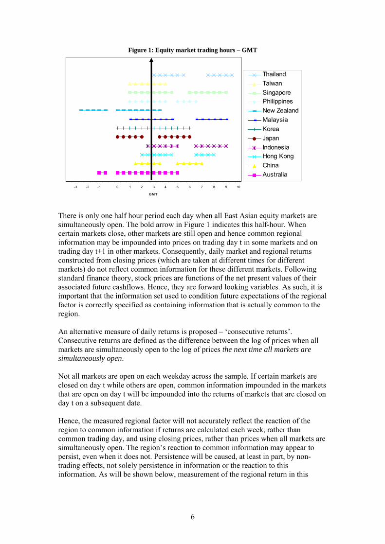
GARCH framework. Section 5 examines whether the regional factors are correctly identified as regional rather than world factors, and Section 6 concludes. 2. Simulated Regional Factors In this Section differences between the trading times of East Asian equity markets are discussed, regional factor and market returns are randomly generated, and the accuracy of different methods of estimating the regional factor is compared. 2.1 Trading Hours A true regional factor measures common movement within a region and can only be measured accurately between times when all markets in the region are open, and hence have been able to react to common regional information. Daily close returns are the standard measure of high frequency returns. They are calculated as the log difference of closing prices on all weekdays in the sample. However, the equity markets in East Asia are open at different times each day. The opening hours of each market are outlined in GMT and local time in Figure 1 and Table 1, respectively.
Table 1: Equity market trading hours – Local time Country
Trading Hours
Half Hour of Overlap (local time) – DST8
Half Hour of Overlap
(local time) Australia 10:00-16:00 14:30 13:30
China 9:30-11:30, 13:00-15:00 11:30 11:30 Hong Kong SAR 10:00-12:30, 14:30-16:00 11:30 11:30
Indonesia 9:30-12:00, 13:30-16:00 10:30 10:30 Japan 9:00-11:00, 12:30-15:00 12:30 12:30 Korea 9:00-15:00 12:30 12:30
Malaysia 9:00-12:30, 14:30-17:00 11:30 11:30 New Zealand 9:30-15:30 15:30 14:30 Philippines 9:00-12:00, 13:00-14:30 11:30 11:30 Singapore 9:00-12:00, 14:00-17:00 11:30 11:30 Thailand 10:00-12:30, 14:30-16:30 10:30 10:30
8 Australia and New Zealand adopt Daylight Savings Time between the first Sunday in October and the last and third last Sunday in March each year, respectively. Local time in these countries is one hour later than during the rest of the year.
6
Figure 1: Equity market trading hours – GMT
-3 -2 -1 0 1 2 3 4 5 6 7 8 9 10
GM T
ThailandTaiwanSingaporePhilippinesNew ZealandMalaysiaKoreaJapanIndonesiaHong KongChinaAustralia
There is only one half hour period each day when all East Asian equity markets are simultaneously open. The bold arrow in Figure 1 indicates this half-hour. When certain markets close, other markets are still open and hence common regional information may be impounded into prices on trading day t in some markets and on trading day t+1 in other markets. Consequently, daily market and regional returns constructed from closing prices (which are taken at different times for different markets) do not reflect common information for these different markets. Following standard finance theory, stock prices are functions of the net present values of their associated future cashflows. Hence, they are forward looking variables. As such, it is important that the information set used to condition future expectations of the regional factor is correctly specified as containing information that is actually common to the region. An alternative measure of daily returns is proposed – ‘consecutive returns’. Consecutive returns are defined as the difference between the log of prices when all markets are simultaneously open to the log of prices the next time all markets are simultaneously open. Not all markets are open on each weekday across the sample. If certain markets are closed on day t while others are open, common information impounded in the markets that are open on day t will be impounded into the returns of markets that are closed on day t on a subsequent date. Hence, the measured regional factor will not accurately reflect the reaction of the region to common information if returns are calculated each week, rather than common trading day, and using closing prices, rather than prices when all markets are simultaneously open. The region’s reaction to common information may appear to persist, even when it does not. Persistence will be caused, at least in part, by non-trading effects, not solely persistence in information or the reaction to this information. As will be shown below, measurement of the regional return in this
7
manner may cause measured autocorrelation and heteroskedasticity in addition to that caused by persistence in the arrival of information.9 The effects of estimating regional factors using close returns, and including days on which regional markets are closed, are examined using the following simulation. The ‘true’ regional factor is generated as a normally distributed random variable with zero mean and a standard deviation of one.
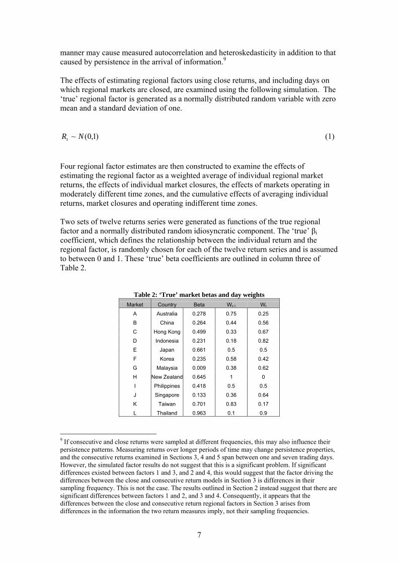
)1,0(~ NRt (1) Four regional factor estimates are then constructed to examine the effects of estimating the regional factor as a weighted average of individual regional market returns, the effects of individual market closures, the effects of markets operating in moderately different time zones, and the cumulative effects of averaging individual returns, market closures and operating indifferent time zones. Two sets of twelve returns series were generated as functions of the true regional factor and a normally distributed random idiosyncratic component. The ‘true’ βi coefficient, which defines the relationship between the individual return and the regional factor, is randomly chosen for each of the twelve return series and is assumed to between 0 and 1. These ‘true’ beta coefficients are outlined in column three of Table 2.
Table 2: ‘True’ market betas and day weights Market Country Beta Wt-1 Wt
A Australia 0.278 0.75 0.25
B China 0.264 0.44 0.56
C Hong Kong 0.499 0.33 0.67
D Indonesia 0.231 0.18 0.82
E Japan 0.661 0.5 0.5
F Korea 0.235 0.58 0.42
G Malaysia 0.009 0.38 0.62
H New Zealand 0.645 1 0
I Philippines 0.418 0.5 0.5
J Singapore 0.133 0.36 0.64
K Taiwan 0.701 0.83 0.17
L Thailand 0.963 0.1 0.9
9 If consecutive and close returns were sampled at different frequencies, this may also influence their persistence patterns. Measuring returns over longer periods of time may change persistence properties, and the consecutive returns examined in Sections 3, 4 and 5 span between one and seven trading days. However, the simulated factor results do not suggest that this is a significant problem. If significant differences existed between factors 1 and 3, and 2 and 4, this would suggest that the factor driving the differences between the close and consecutive return models in Section 3 is differences in their sampling frequency. This is not the case. The results outlined in Section 2 instead suggest that there are significant differences between factors 1 and 2, and 3 and 4. Consequently, it appears that the differences between the close and consecutive return regional factors in Section 3 arises from differences in the information the two return measures imply, not their sampling frequencies.

8
The first set of return series assumes that all markets close at the same time. This series is equivalent to a ‘consecutive’ return series. This is generated as follows.
)1,0(~, ,,,,1 NRr titititi εεβ += (2)
The second set of return series relaxes the assumption that all twelve markets close at the same time. The twelve equity markets of East Asia open and close at different local times, open for different periods of time, and operate in different time zones. They are only simultaneously open for, at most, thirty minutes each day. This period of ‘common openness’ is between 0300 and 0330 GMT. The proportion of each day’s trading that occurs in each market before and after 0300-0330 are denoted wi,t-1 and wi,t, respectively, with wi,t-1 and wi,t summing to one. The weights of each Asian equity market are associated with each of the twelve randomly generated series following alphabetic order as shown in columns four and five of Table 2. True market returns were then calculated as functions of the true regional beta and the weighted average of the true regional return on the day before 0300 GMT, return t-1, and the day after 0300, return t. Specifically,
)1,0(~,)( ,,11,,2 NRwRwr titittttiti εεβ ++= −− (3)
Return series 1, tir ,,1 , is a series of returns constructed between times when all markets are open and trading. They are equivalent to a ‘consecutive’ return series. Return series 2, tir ,,2 , is a series of returns calculated using individual markets’ closing prices on days on which all markets in the region are open for trading. They are equivalent to a standard close returns series with non-trading days excluded. Two further sets of twelve return series were constructed to examine the effects of market closures. The working days between 1 July 1997 and 30 September 2002 during which each East Asian equity market was closed are incorporated by substituting a zero for the return of the randomly generated series at the relevant data point. The market closures of each Asian equity market are again associated with each of the twelve randomly generated series following alphabetic order.10The patterns of zero returns from the twelve East Asian equity markets examined in this analysis were imposed on the first set of twelve return series to yield return series 3, tir ,,3 , and on the second set of twelve return series to yield return series 4, tir ,,4 . Return series 3 is a series of returns constructed between times when all markets are generally, but not necessarily, open. Individual market closures are not eliminated
10 Australia=a, China=b, Hong Kong=c, Indonesia=d, Japan=e, Korea=f, Malaysia=g, New Zealand=h, Philippines=i, Singapore=j, Taiwan=k, and Thailand=l.

9
from return series 3. Return series 4 is a series of returns calculated using individual market closing prices, on all days when markets are generally, although not necessarily, open. At each point in time, four ‘estimated’ regional factors are calculated as equally-weighted combinations of the four sets of twelve returns
∑=
==12
1,,, 4,3,2,1,
121ˆ
itijtj jrR (4)
The descriptive statistics of the four estimated regional factors, and of the true regional factor are outlined in Table 3.
Table 3: Regional factor descriptive statistics True Factor 1 Factor 2 Factor 3 Factor 4
Mean -0.001 0.01 0.016 0.011 0.017
Maximum 3.353 1.478 1.417 1.478 1.417
Minimum -3.491 -1.954 -1.312 -1.874 -1.275
Std. Dev. 0.997 0.51 0.417 0.49 0.4
Skewness -0.069 -0.092 0.021 -0.066 0.041
Kurtosis 3.026 3.045 3.018 3.11 3.078
Estimating the regional factor as a weighted-average of individual market returns underestimated the true variability of the regional factor, which is not surprising since it is an average, while the inclusion of non-trading days does not seem to greatly affect the characteristics of the return series. However, when markets are assumed to close at different times (as for factors 2 and 4), the estimated factors are positively, rather than negatively, skewed. Correlations between these four estimated regional factors and the true regional factor are provided in Table 4.
Table 4: Estimated regional factor correlations Factor 1 Factor 2 Factor 3 Factor 4 True
Factor 1 1 0.408 0.986 0.407 0.832
Factor 2 0.408 1 0.407 0.984 0.495
Factor 3 0.986 0.407 1 0.409 0.821
Factor 4 0.407 0.984 0.409 1 0.495
True 0.832 0.495 0.821 0.495 1 The correlations between factors 1 and 2, and factors 3 and 4, are much lower than the correlations between factors 1 and 3, and factors 2 and 4, suggesting that the type of returns used to define the factors, rather than the inclusion of non-trading days, drives differences between the regional factor models. The correlations of estimated regional factors 2 and 4 with the true regional factor are much lower than those of estimated regional factors 1 and 3. This is to be expected. Regional factors 1 and 3 are

10
calculated at each point in time using returns which are functions of the true factor at the same point in time, while factors 2 and 4 are calculated at each point in time using returns which are functions of the true factor at both that point in time, and the previous time period. The effects of the way returns are constructed on the autoregressive and variance properties of the estimated regional factors are examined using a AR(1) GARCH(1,1) framework.11 This specification models returns as first-order autoregressive processes, with conditional variances that vary with time. The return and variance properties of each regional factor estimate are compared to those of the true randomly generated regional factor using the following framework. The four estimated regional factors are modelled as in Equation (5) and the estimated return and variance parameters are compared to the true regional factor return and variance parameters, modelled as in Equation (6).
21,
21,
2,
2,,,1,,
ˆˆˆˆˆˆ
)ˆ,0(~ˆ,ˆˆˆ
−−
−
++=
++=
tjjtjjjtj
tjtjtitjjitj NRR
σγεαφσ
σεεβς (5)
j=1,2,3,4
21
21
2
21 ),0(~,
−−
−
++=
++=
ttt
ttttt NRR
γσαεφσ
σεεβς (6)
The estimated and actual parameters are outlined in columns two to six of Table 5.
11 A GARCH(1,1) model has two distinct specifications - one for the conditional mean and one for the conditional variance. In this case, the conditional mean is specified as a first-order autoregressive process and an error term. The variance of the error term is made conditional upon news about volatility from the previous period, measured as the lag of the squared residual from the mean equation, the ARCH term, and the previous period’s forecast variance, the GARCH term.

11
Table 5:Comparison of actual and estimated regional factor return and variance parameters12 Return Variance Wald Tests13
C(1) AR(-1) C ARCH(1) GARCH(1) Return Variance Overall
TRUE 0.001 0.003 0.73 0.039 0.226 0.008 0.685 0.358 [0.974] [0.901] [0.282] [0.262] [0.745] [0.992] [0.504] [0.839]
Factor 1 0.012 0.018 0.015 -0.018 0.961 0.673 1.810 1.179 [0.366] [0.462] [0.220] [0.058] [0] [0.510] [0.164] [0.318]
Factor 2 0.012 0.249 0.052 0.016 0.665 48.631 0.175 24.342
[0.247] [0] [0.665] [0.563] [0.379] [0] [0.84] [0]
Factor 3 0.011 0.028 0.036 -0.013 0.863 1.043 0.308 0.694 [0.378] [0.256] [0.572] [0.434] [0.001] [0.353] [0.735] [0.596]
Factor 4 0.012 0.246 0.036 0.013 0.747 47.461 0.173 23.800
[0.217] [0] [0.658] [0.566] [0.179] [0] [0.841] [0]
The true regional factor was randomly generated from a normal distribution with mean zero and variance of one. This implies that the true trend and autoregressive regional return parameters, and variance ARCH(1) parameter are insignificantly different from zero, and that the sum of the variance constant and GARCH(1) parameters is insignificantly different from unity. Consequently, the estimated return trend and AR(1), and variance ARCH(1) parameters of any estimate of the true regional trend should be insignificantly different from zero, and the sum of the estimated GARCH(1) and variance constant coefficients should be insignificantly different from unity. Three Wald tests, for the return specification, variance specification and the joint return and variance specification, are calculated. These test results are shown in columns eight, nine and ten of Table 5. The Wald test results suggest that modelling the true regional factor as AR(1) GARCH(1,1) does not, in itself, effect the true regional factor’s estimated characteristics. Further, estimating regional factors using a weighted-average of individual market consecutive returns does not appear to introduce errors in either the return or variance specifications. Alternatively, estimating regional factors using close returns introduces substantial and spurious autoregressive return properties.14 On this basis, modelling the regional factor as a AR(1) GARCH(1,1) process does not in itself bias the estimated characteristics of the regional factor, regional factors defined using consecutive returns appear to be less biased than close returns defined factors, and
12 C(1) and AR(-1) are the estimated return constant and first-order autoregressive coefficient,
ji βς ˆ&ˆ , respectively, while C, ARCH(1) and GARCH(1) are the estimated variance constant,
ARCH(1) and GARCH(1) parameters, γαφ ˆ&ˆ,ˆjj , respectively .
13 The bolded Wald Test figures denote an inability to reject null hypothesis that coefficients are as predicted 14 It is interesting that the significant autoregressive coefficients for both close factors, 2 and 4, are approximately 0.25. Working (1960) shows that the use of averages can introduce correlations not present in the original series. The expected first-order correlation of first differences between averages of terms in a random chain approximates 0.25 even when the number of elements being averaged is fairly small. However, if the positive autocorrelation displayed in Table 5 was a function of the averaging of individual return series, factors 1 and 3 would also exhibit positive, significant autocorrelation of approximately 0.25. They do not. Consequently, while the estimated autoregressive coefficients for factors 2 and 4 are remarkably similar to those predicted by Working (1960), this would appear to be due to coincidence rather than causation.

12
failure to explicitly account for individual market closures does not appear to greatly influence the quality of regional factor estimation.15 3. Consecutive and Close Return Regional Factors The return series used to estimate regional factors effects the quality of regional factor estimate. The form of index weighting used to construct the regional factor may also affect the properties and quality of the estimated regional factor. Attention is now turned to equity market data, and the effects of market capitalisation, as opposed to equal- or principal component-weightings, on the characteristics of estimated regional factors.16 The data sample covers half-hour prices for the headline equity indices of Australia, China,17 Indonesia, Malaysia, Korea, Japan, New Zealand, Philippines, Singapore, and Thailand on each trading day between 1 January 1997 and 30 September 2002. These equity indices are denoted by country name. Daily close returns are the standard measure of high frequency returns. As noted above, they are calculated as the log difference of closing prices on all weekdays in the sample. These returns are equivalent to the simulated return series 4, tir ,,4 , in Section 2. However, a true regional factor measures common movement within a region and can only be accurately measured between times when all markets have been open, and hence have been able to react to common regional information. An alternative measure of returns is proposed – ‘consecutive returns’. Consecutive returns are defined as the difference between the log of prices when all markets are simultaneously open to the log of prices the next time all markets are simultaneously open. Unlike close returns, consecutive returns are not equivalent in terms of the time intervals they represent.18 Rather, they are equivalent in terms of the minimum information that they contain – all consecutive day returns contain information revealed during at least one full trading day in each market.19 These returns are similar to the simulated return series 1, tir ,,1 , in Section 2. Regional factors are constructed from consecutive returns and from close returns using three forms of weighting –
15 It is not immediately obvious why including returns from days when markets are closed does not appear to affect the properties of the estimated regional factor. All markets in East Asia were open on only 68.4% of days in the sample. On 18.6% one market out of twelve was closed, and on 13% of days more than one market was closed. 16 Actual data is used for this analysis as simulations impose a ‘true’ regional weight for each market. Hence, the factor weighting that is closest to this arbitrarily imposed set of ‘true’ weights will outperform other weights – no additional information can be implied. 17 The selected Chinese Index is the Shanghai A Index. This index can not be traded by foriegners. 18 Within this sample, consecutive returns cover between one trading day and ten trading days (typically during common holiday periods such as Chinese New Year). In total, the sample provides 639 consecutive returns, compared with 974 closing price returns (which include days on which one or more regional market is closed). 19 Thus, consecutive returns do not suffer from an intuitive problem with daily close price return series. Daily return series treat the return between Friday and Monday identically to the return between Monday and Tuesday, when they are clearly not equivalent in terms of the time periods they represent.

13
equal (as in Section 2), market-capitalisation and principal component20 weights, and the characteristics of these estimated factors are compared. 3.1 Factor Construction The weightings for each factor are presented in Table 6.
Table 6: Normalized factor weightings21 Principal Component Market Equal
Index Consecutive Close Capitalisation
Australia 0.11 0.13 0.15 0.1
China 0 0.01 0.09 0.1
Indonesia 0.09 0.08 0 0.1
Malaysia 0.08 0.09 0.03 0.1
Korea 0.13 0.12 0.05 0.1
Japan 0.11 0.12 0.6 0.1
New Zealand 0.1 0.11 0 0.1
Philippines 0.1 0.1 0.01 0.1
Singapore 0.15 0.14 0.05 0.1
Thailand 0.12 0.11 0.01 0.1
For each market, the principal component weights applied to the close and consecutive series are approximately equivalent, and are similar to those of the equal factor for all markets except China.22 Indonesia, Malaysia, Korea, New Zealand, Philippines, Singapore and Thailand have much lower market capitalisation factor weights than equal or principal component-weights, while the market capitalisation factor attributes a much higher weighting to Japan, 0.6 compared with 0.11, and China, 0.09 compared with 0, than the principal components factor. Descriptive statistics for each of the nine regional factors are displayed in Table 7.
Table 7: Regional factor descriptive statistics Statistics Consecutive Close
Equal Mean 0 0
Maximum 0.056 0.03
Minimum -0.064 -0.062
Std. Dev. 0.011 0.008
Skewness 0.02 -0.99
Kurtosis 8.647 9.382
20 Principal component weights are extracted using a variance maximizing rotation of the original variable space. This type of rotation is called variance maximizing because the criterion for (goal of) the rotation is to maximize the variance (variability) of the "new" variable (principal component), while minimizing the variance around the new variable 21 Principal component factor weightings are normalized to sum to unity, and the cumulative proportion of variation explained is 0.35 for consecutive returns and 0.33 for close returns. 22 The negligible principal component weighting for China is in line with previous work examining common factors in Asia. De Brouwer (2002) provides discussion of why this occurs.

14
Observations 63923 974
Market Capitalisation Mean 0 0
Maximum 0.045 0.037
Minimum -0.058 -0.056
Std. Dev. 0.011 0.009
Skewness -0.148 -0.322
Kurtosis 5.925 5.828
Observations 639 974
Principal Component Mean 0 0
Maximum 9.679 6.557
Minimum -12.232 -14.706
Std. Dev. 1.875 1.815
Skewness -0.253 -1.245
Kurtosis 9.471 11.038
Observations 639 973
Across all three types of factor weighting, the close factors display greater positive skewness than the consecutive factors. Otherwise, the equal and market capitalisation factors display similar characteristics, with one exception – the equal factors display greater leptokurtosis than their market capitalisation counterparts. 3.2 GARCH Characteristics of Regional Factors The GARCH characteristics of these series are examined by estimating AR(1) GARCH(1,1) models for each factor. These models are in the form:
(7)
Rn,j,,t is the regional factor with n representing the type of weighting (equal, market capitalisation or principal component) and j representing the type of return (consecutive or close). The estimated return and variance specification parameters are outlined in Table 8.
23 The Consecutive return series only includes observation from days on which all markets in the region are open and trading. The close return series includes all weekdays in the sample, and hence includes days on which certain markets are closed.
21,,,
2,,
2
2,,,,1,,,,,,
1,,,,
,,),0(~;
−
−
++=
++=
− tjnjnRjnjnR
Rtjntjntjnjnjntjn
tjntjn
tjnNRR
εψσςϕσ
σεερα
15
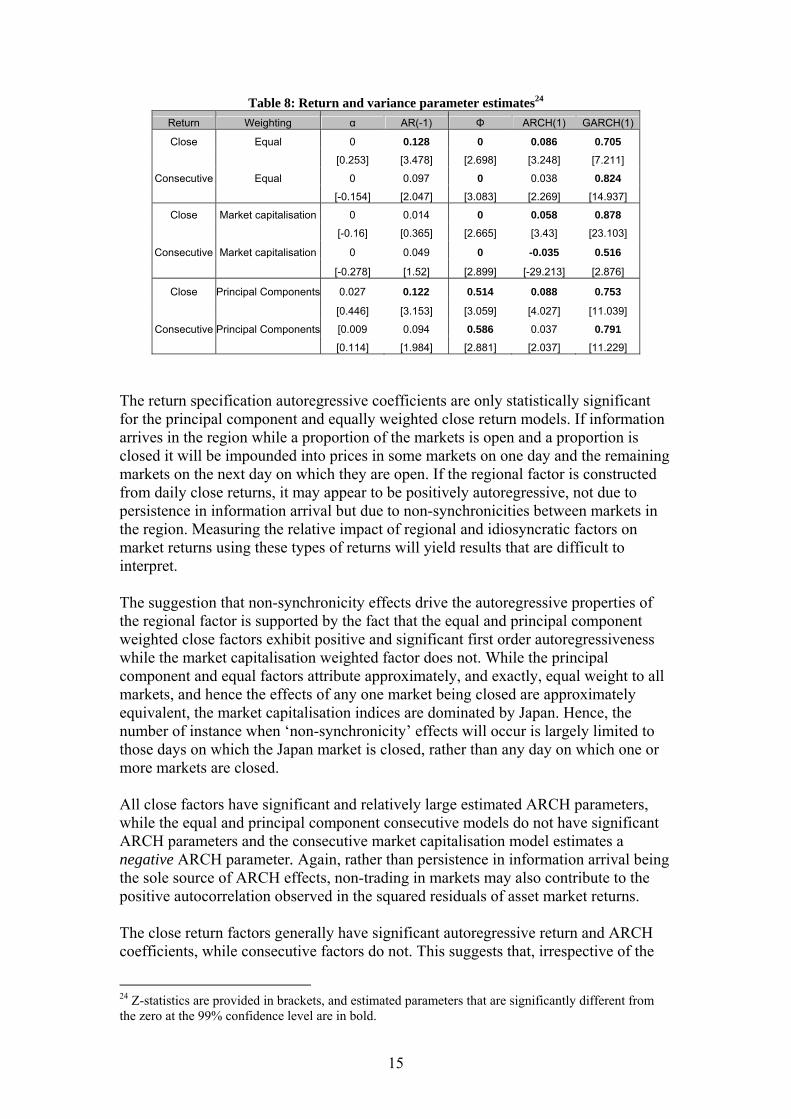
Table 8: Return and variance parameter estimates24 Return Weighting α AR(-1) Φ ARCH(1) GARCH(1)
Close Equal 0 0.128 0 0.086 0.705 [0.253] [3.478] [2.698] [3.248] [7.211]
Consecutive Equal 0 0.097 0 0.038 0.824 [-0.154] [2.047] [3.083] [2.269] [14.937]
Close Market capitalisation 0 0.014 0 0.058 0.878 [-0.16] [0.365] [2.665] [3.43] [23.103]
Consecutive Market capitalisation 0 0.049 0 -0.035 0.516
[-0.278] [1.52] [2.899] [-29.213] [2.876]
Close Principal Components 0.027 0.122 0.514 0.088 0.753
[0.446] [3.153] [3.059] [4.027] [11.039]
Consecutive Principal Components [0.009 0.094 0.586 0.037 0.791 [0.114] [1.984] [2.881] [2.037] [11.229]
The return specification autoregressive coefficients are only statistically significant for the principal component and equally weighted close return models. If information arrives in the region while a proportion of the markets is open and a proportion is closed it will be impounded into prices in some markets on one day and the remaining markets on the next day on which they are open. If the regional factor is constructed from daily close returns, it may appear to be positively autoregressive, not due to persistence in information arrival but due to non-synchronicities between markets in the region. Measuring the relative impact of regional and idiosyncratic factors on market returns using these types of returns will yield results that are difficult to interpret. The suggestion that non-synchronicity effects drive the autoregressive properties of the regional factor is supported by the fact that the equal and principal component weighted close factors exhibit positive and significant first order autoregressiveness while the market capitalisation weighted factor does not. While the principal component and equal factors attribute approximately, and exactly, equal weight to all markets, and hence the effects of any one market being closed are approximately equivalent, the market capitalisation indices are dominated by Japan. Hence, the number of instance when ‘non-synchronicity’ effects will occur is largely limited to those days on which the Japan market is closed, rather than any day on which one or more markets are closed. All close factors have significant and relatively large estimated ARCH parameters, while the equal and principal component consecutive models do not have significant ARCH parameters and the consecutive market capitalisation model estimates a negative ARCH parameter. Again, rather than persistence in information arrival being the sole source of ARCH effects, non-trading in markets may also contribute to the positive autocorrelation observed in the squared residuals of asset market returns. The close return factors generally have significant autoregressive return and ARCH coefficients, while consecutive factors do not. This suggests that, irrespective of the
24 Z-statistics are provided in brackets, and estimated parameters that are significantly different from the zero at the 99% confidence level are in bold.

16
weighting technique, close return defined regional factor estimates may be affected by the non-synchronicity of regional trading. Subsequent analysis will focus on consecutive returns. Estimating regional factors using close returns has been shown using both simulated and actual market data to introduce positive first order autoregressiveness. This suggests that mismeasurement of the regional factor may indeed lead to spurious conclusions regarding the region’s influence on individual market returns. Section 4 estimates the influence of the East Asian regional factor on East Asian equity markets’ returns. 4. Market Returns and Market-Specific Regional Factors As noted in Section 1, common information will affect equity markets within a region through two broad mechanisms – financial and trade linkages. However, regional factors constructed from closing prices (which are taken at different times for different markets) do not reflect common information for these different markets. Further, the results of Sections 2 and 3 suggest that calculating regional factors using close returns appears to affect the statistical properties of the resulting estimates. In this Section, market specific factors are constructed using consecutive, rather than close, returns. The return and conditional variance characteristics of East Asian equity markets’ consecutive returns and their associated consecutive regional factors, and the correlations between these return and factor measures, are examined. 4.1 Consecutive market returns and Market Specific Factor Characteristics The equal and principal component weights are similar for all markets except China, and the characteristics of regional factors estimated using these weightings is shown in Section 3 to be very similar. Principal component weights, rather than equal weights, are chosen for further analysis, as the principal component weighting for China is approximately zero. This provides an extreme example of a market whose return does not contribute to a regional factor. This is in stark contrast to the market capitalisation weighted factors, in which Japanese returns account for approximately 60% of the weighting. Individual markets’ consecutive returns are used to construct principal component and market capitalisation regional factors for each market. The regional factor for each market is calculated as comprising all markets in the region except the market that it is to explain.25 Descriptive statistics for these ten regional factors, and the ten individual market return series are outlined in Table 9. The ten principal component factors have similar characteristics, as expected given that the principal component weights are approximately equal. The market capitalisation factors have similar characteristics, except for Japan. While the
25 If the regional factor includes all markets in the region, this introduces problems associated with endogeneity. To use a working example; if this form of regional factor is calculated using market capitalisation weights and is used to explain Japan returns, Japan returns are being explained by contemporaneous measures of regional returns that comprise approximately 60 percent of the same (contemporaneous) Japan returns. Using this measure, one would expect the ‘regional’ factor to explain 60 percent of Japan returns, even if Japan returns are unaffected by the region.

17
remaining market factors have small negative mean returns, the Japan regional factor has a small positive mean, a smaller range and standard deviation, is more positively skewed and displays more leptokurtosis. The ten market return series have similar standard deviations. Further, except for Australia and New Zealand, market returns, particularly those of Japan and Korea, have higher standard deviations than their corresponding factors. This suggests that Japan and Korea have relatively large idiosyncratic components while the idiosyncratic proportion of return variation in Australia and New Zealand is small.
Table 9: Market and market-specific factor descriptive statistics
The correlations between the two regional factors and market return for each market are outlined in Table 10.
Australia China Indonesia Malaysia Korea Japan New
Zealand Philippines Singapore Thailand
Individual Market’s Consecutive Returns
Mean 0.000 0.000 0.000 0.000 0.000 -0.001 0.000 -0.001 0.000 0.000
Maximum 0.035 0.086 0.134 0.130 0.116 0.081 0.039 0.163 0.087 0.160
Minimum -0.068 -0.087 -0.163 -0.108 -0.153 -0.080 -0.064 -0.088 -0.078 -0.140
Std. Dev. 0.009 0.018 0.024 0.018 0.030 0.018 0.010 0.019 0.018 0.023
Skewness -0.571 0.314 0.326 0.553 -0.118 -0.054 -0.416 1.239 0.444 0.158
Kurtosis 8.858 7.196 11.062 11.516 6.161 5.236 7.197 18.411 6.963 9.579
Consecutive returns, Principal Component-Weighted Factors
Mean 0.000 0.000 0.000 0.000 0.000 0.000 0.000 0.000 0.000 0.000
Maximum 0.090 0.097 0.095 0.098 0.091 0.092 0.094 0.074 0.100 0.088
Minimum -0.102 -0.122 -0.122 -0.119 -0.111 -0.114 -0.107 -0.120 -0.119 -0.126
Std. Dev. 0.018 0.019 0.018 0.018 0.018 0.018 0.018 0.018 0.017 0.018
Skewness 0.026 -0.253 -0.366 -0.289 -0.206 -0.213 -0.014 -0.373 -0.315 -0.339
Kurtosis 9.023 9.472 9.540 9.621 9.493 9.624 8.489 8.810 10.473 9.971
Consecutive returns, Market-Capitalisation-weighted Factors
Mean 0.000 0.000 0.000 0.000 0.000 0.000 0.000 0.000 0.000 0.000
Maximum 0.046 0.044 0.044 0.045 0.040 0.014 0.045 0.044 0.045 0.044
Minimum -0.050 -0.058 -0.058 -0.057 -0.052 -0.020 -0.058 -0.058 -0.056 -0.058
Std. Dev. 0.010 0.011 0.011 0.011 0.010 0.003 0.011 0.011 0.011 0.011
Skewness -0.060 -0.163 -0.146 -0.139 -0.143 -0.246 -0.146 -0.150 -0.144 -0.148
Kurtosis 5.589 6.008 5.910 5.848 5.587 7.680 5.908 5.847 5.927 5.903

18
Table 10: Correlations between market returns and regional factors26 Market Returns
Market Capitalisation
Principal Component
Australia 0.489 0.492 China 0.019 -0.006
Japan 0.532 0.487 Indonesia 0.201 0.381 Malaysia 0.215 0.347
Korea 0.551 0.595 New Zealand 0.344 0.433 Philippines 0.249 0.442 Singapore 0.498 0.699 Thailand 0.331 0.526
Australia, Japan, Korea, and Singapore, the most developed markets in this analysis, are highly positively correlated with their respective market capitalisation-weighted factors. The market with the greatest market capitalisation weight after Japan is Australia – Australia returns comprise approximately 37.5 percent of the market capitalisation-weighted regional factor for Japan, while the Japan market’s returns comprise approximately 70 percent of the Australia market capitalisation factor. The Japan market is less correlated with its principal component-weighted regional factor, while the Australia market is (approximately) as correlated with its principal component factor. This may suggest that they are either influenced significantly by one another’s returns or, particularly in the case of Japan, that these developed markets are being influenced by a common world factor, proxied in part by the market capitalisation regional factors calculated in this analysis. Alternatively, the correlations of Korea and, particularly, Singapore are even higher with their principal component factors than their market capitalisation factors. The principal component factors are far less influenced by Australia and Japan returns. This suggests that these markets may be influenced by both world and regional influences. The correlations of the remaining markets’ returns and their respective principal component factors are much higher than with their market capitalisation factors except for China, which is uncorrelated with either factor, and New Zealand, for which it is still higher. The markets that are more correlated with their principal component factors represent, with the exclusion of China, the least developed markets in this study. 4.2 GARCH Characteristics of Market Returns and Market-Specific Factors The GARCH characteristics of the twenty principal component and market capitalisation regional factors and the ten market return series are examined by estimating individual AR(1) GARCH(1,1) specifications as follows;
26 Bold denotes significance at the 99 percent confidence level.

19
Regional Factors
(8)
Individual market returns
21,
21,
2,
2,,,1,, ),0(~;
−−
−
++=
++=
tiitiiiti
titititiiiti Nrr
εψσςϕσ
σεεβα
(9)
Rn,j,t is the regional factor with n representing the type of weighting (market capitalisation or principal component) and j representing the factor calculated from all markets except market i.. The estimated conditional variance series from these regressions are identified as 2
, jnRσ . The individual market returns is ri , with i representing the market (Australia, China, Indonesia, Japan, Korea, Malaysia, New Zealand, Philippines, Singapore, or Thailand). The estimates for the individual markets are presented in Table 11. As with the general consecutive market capitalisation and principal component factors outlined in Section 3, no market specific factors have significant first order autoregressive return coefficients.
Similarly, only Malaysia’s market return has an estimated autoregressive return coefficient that is significant. Most markets’ estimated conditional variance specifications have significant ARCH and GARCH parameters, except for Indonesia and Thailand which have insignificant GARCH parameters, and Korea which has an insignificant ARCH parameter. However, only the New Zealand principal component and Malaysia market capitalisation factors have significant ARCH coefficients in their estimated variance specifications (and the estimated Malaysia parameter is negative).
21,,
2,,
2
2,,1,,1,,,,,,
1,,,,
,,),0(~;
−
−−
++=
++=
− tjnRjnjnR
Rtjntjntjnjnjntjn
tjntjn
tjnNRR
ψεσςϕσ
σεερα

20
Table 11: Estimated AR(1) GARCH(1,1) specifications27 Market Return Variance
C(1) AR(-1) C ARCH(1) GARCH(1)
Principal Components Factor
Australia 0 0.083 0.377 0.034 0.844 [-0.001] [1.758] [2.869] [2.21] [15.93]
China 0.009 0.094 0.587 0.037 0.791 [0.114] [1.985] [2.884] [2.039] [11.228]
Indonesia 0.013 0.088 0.484 0.028 0.822 [0.163] [1.872] [2.079] [1.512] [9.699]
Malaysia 0.009 0.085 0.503 0.032 0.814 [0.118] [1.866] [2.621] [1.727] [11.433]
Korea 0.007 0.089 1.048 0.053 0.595 [0.098] [1.877] [2.346] [2.298] [3.639]
Japan 0.016 0.112 0.38 0.056 0.823 [0.202] [2.353] [4.382] [3.27] [21.126]
New Zealand 0.005 0.104 0.425 0.035 0.83 [0.062] [2.248] [2.861] [2.204] [14.52]
Philippines 0.012 0.092 0.612 0.042 0.765 [0.153] [1.898] [2.541] [1.996] [8.586]
Singapore 0.01 0.097 0.498 0.033 0.794 [0.136] [2.001] [2.534] [1.723] [9.878]
Thailand 0.004 0.077 1.003 0.029 0.647 [0.053] [1.625] [1.453] [1.337] [2.746]
Market Capitalisation-Weighted Factor
Australia 0 0.027 0 0.021 0.893 [-0.508] [0.573] [1.013] [1.516] [9.372]
China 0 0.033 0 0.021 0.885 [-0.515] [0.68] [0.99] [1.448] [8.363]
Indonesia 0 0.044 0 -0.036 0.501
[-0.518] [1.289] [2.449] [-2.539] [2.43]
Malaysia 0 0.044 0 -0.037 0.397
[-0.365] [1.263] [2.581] [-4.943] [1.63]
Korea 0 0.031 0 0.017 0.889 [-0.564] [0.655] [0.894] [1.3] [7.784]
Japan 0 0.104 0 0.032 0.828 [0.356] [2.396] [1.791] [2.083] [9.323]
New Zealand 0 0.034 0 -0.037 0.16
[-0.525] [1.035] [2.423] [-2.439] [0.448]
Philippines 0 0.034 0 0.015 0.881 [-0.468] [0.721] [0.728] [1.06] [5.746]
Singapore 0 0.032 0 0.017 0.896 [-0.479] [0.662] [0.859] [1.319] [8.058]
Thailand 0 0.03 0 0.017 0.904 [-0.468] [0.624] [0.904] [1.334] [9.298]
Market Returns
Australia 0.035 0.088 0 0.132 0.742 [0.961] [1.847] [2.628] [4.563] [10.694]
27 Z-statistics are provided in brackets, and estimated parameters that are significantly different from the zero at the 99% confidence level are in bold.

21
China 0.0448 0.067 0 0.171 0.823 [0.877] [1.353] [4.354] [7.236] [41.933]
Indonesia -0.0953 0.058 0 0.251 0.151
[-0.968] [1.005] [8.599] [6.754] [2.067]
Malaysia 0.0122 0.169 0 0.08 0.907 [0.188] [3.936] [3.685] [8.363] [86.661]
Korea 0.00309 0.012 0 0.022 0.926 [0.025] [0.243] [1.52] [2.202] [22.438]
Japan -0.0359 0.011 0 0.028 0.952 [-0.493] [0.246] [1.998] [3.084] [56.736]
New Zealand -0.00492 -0.001 0 0.065 0.894 [-0.124] [-0.012] [2.567] [3.874] [31.006]
Philippines -0.076 0.113 0 0.068 0.894 [-1.006] [2.501] [4.446] [5.139] [49.141]
Singapore -0.0133 0.074 0 0.045 0.894 [-0.18] [1.761] [5.981] [4.691] [60.959]
Thailand -0.1354 0.072 0 0.289 0.085 [-1.637] [1.529] [8.038] [4.34] [0.949]
The principal component factor model GARCH coefficients of all markets are significant, and, with the exceptions of Korea and Thailand, these coefficients are all relatively high. The GARCH coefficients of the market capitalisation factor models are significant and high, except for those of Indonesia, Malaysia and New Zealand, which are insignificant. In fact, the market capitalisation models for these markets exhibit neither the significant (positive) ARCH or GARCH coefficients commonly associated with (close price defined) asset returns. The factors and markets in the region appear to be heterogenous. While most markets have significant ARCH and GARCH parameters, eighteen of the twenty regional factor measures do not possess significant ARCH parameters. Further, while the market capitalisation and principal component factors for Thailand, and the principal component factor for Indonesia, have significant estimated GARCH parameters, the market returns of Indonesia and Thailand do not. Consequently, each market is individually modelled as a function of its regional factor and an idiosyncratic component which follows a GARCH(1,1) process. The estimated conditional variance series of each model comprises the time varying conditional variance of the regional factor and the time varying conditional variance of the idiosyncratic component. 5. Idiosyncratic and Regional Effects on East Asian Equity Markets In this Section, the contributions of regional and idiosyncratic influences on market returns and conditional variances are examined. Regional and idiosyncratic effects are allowed to differ between markets, and the relative influence of the region is compared across markets.

22
5.1 Idiosyncratic and Regional Contributions to Market Returns The following model is estimated:
21,,,
21,,,,
2,,
2,,,,,,,,,,,, ),0(~;
−− ++=
++=
tinintininintin
tintintintjninintin NRr
εψσςϕσ
σεεβα
(10)
where n represents the type of weighting (market capitalisation or principal component), i represents the market return being modelled (Australia, China, Indonesia, Japan, Korea, Malaysia, New Zealand, Philippines, Singapore, or Thailand), and j represents the factor calculated from all markets except market i. The estimated parameters of these models are presented Table 12.
Table 12: Estimated return and variance parameters28 Market Return Variance
C(1) Region C ARCH(1) GARCH(1) Adj-R2
Principal Component Weighted Australia 0 0.234 0 0.199 0.228 0.236
[0.068] [26.323] [5.737] [4.139] [1.759] China 0.001 0 0 0.171 0.821 -0.006
[1.024] [0.011] [4.419] [7.021] [41.493] Indonesia 0 0.426 0 0.293 0.079 0.148
[-0.463] [11.980] [8.381] [6.683] [0.963] Malaysia [0.001 0.323 0 0.125 0.858 0.114
[0.845] [14.734] [5.368] [11.441] [82.184] Korea 0 1.058 0 -0.005 1.003 0.349
[0.118] [33.746] [0.464] [-222.445] [1913.946] Japan 0 0.469 0 0.028 0.962 0.231
[-0.506] [20.124] [1.592] [3.311] [72.156] New Zealand 0 0.243 0 0.051 0.934 0.183
[-0.104] [19.448] [1.563] [3.978] [49.541] Philippines -0.001 0.495 0 0.247 0.573 0.189
[-1.486] [21.124] [6.306] [7.857] [13.69] Singapore 0 0.705 0 0.047 0.917 0.484
[-0.122] [36.211] [3.689] [3.486] [53.786] Thailand 0.001 0.629 0 -0.007 1.001 0.27
[0.959] [20.846] [5.156] [-55.151] [1485.048] Market Capitalisation Weighted
Australia 0 0.4 0 0.161 0.564 0.233
28 Z-statistics are provided in brackets, and estimated parameters that are significantly different from the zero at the 99% confidence level are in bold.

23
[1.076] [23.537] [4.05] [4.332] [6.091] China 0.001 0.005 0 0.171 0.821 -0.006
[1.027] [0.099] [4.414] [7.028] [41.505] Indonesia 0 0.408 0 0.294 0.024 0.038
[-0.468] [6.705] [13.628] [7.242] [0.447] Malaysia 0.001 0.284 0 0.092 0.89 0.038
[0.763] [6.883] [4.55] [9.83] [83.343] Korea 0.001 1.624 0 -0.002 1.004 0.299
[1.096] [24.268] [-1.584] [-28.371] [721.563] Japan -0.001 2.875 0 0.048 0.913 0.277
[-1.239] [18.931] [1.921] [3.601] [30.985] New Zealand 0 0.284 0 0.05 0.917 0.112
[0.207] [12.656] [2.081] [3.246] [33.926] Philippines -0.001 0.437 0 0.088 0.847 0.056
[-1.171] [9.524] [5.201] [7.156] [40.897] Singapore 0 0.773 0 0.103 0.828 0.241
[0.69] [22.086] [4.018] [5.802] [34.147] Thailand 0.001 0.639 0 -0.014 1.002 0.102
[1.173] [11.131] [3.954] [-3.41] [461.334] The market returns are positively and significantly related to their respective market capitalisation factors in all markets except China. The estimated coefficients are lowest for New Zealand and Malaysia, and are substantially larger for Japan and Korea than for any other markets. Table 9 suggests a possible reason for this. The standard deviations of the Japan and Korea market capitalisation factors are much smaller than the standard deviations of their market returns. This is not true for the other markets. The estimated coefficients for the principal component factors are more similar. With the exception of China, they are all positive and significant and range from 0.002 to 0.011. The market capitalisation factor coefficients range from 0.284 to 2.875. The ARCH and GARCH parameters are significant, positive and of approximately the size commonly estimated for daily asset return series in seven of the ten market capitalisation models and six of the ten principal component models.29 The market capitalisation and principal component Indonesia GARCH parameter estimates are insignificant and the Korea and Thailand models have GARCH parameters in excess of one and negative ARCH parameters. Further, the estimated principal component Australia GARCH parameter is insignificant and the market capitalisation Korea model’s estimated variance specification is explosive. The adjusted R2 of the market capitalisation models suggest that these are good representations of the developed markets of Singapore, Japan, Korea and Australia, and are poor models for the less developed markets of Thailand, Philippines,
29 There is a wide body of literature concerning GARCH models estimated with daily asset returns. See, for example, the work by Tim Bollerslev in this area.

24
Malaysia, and Indonesia. These models explain more of the variation in the returns of the developed markets in the region than in the returns of the less developed nations of the region. This may suggest that developed markets are more influenced by Japan returns than the developing markets in Asia. The adjusted R2 of the principal component models suggest that these representations explain much more of the variation in the returns of the least developed markets than the market capitalisation models. This suggests that these markets are influenced more by one another than by Japan, the largest market in the region. The developed markets’ principal component models explain approximately the same proportion of variation as their market capitalisation models, with the exception of Singapore. The principal component model explains substantially more of the variation in Singapore market returns than the market capitalisation model. These results suggest that developed markets may react to a world factor, proxied in this analysis by the two measures of regional factor, while the least developed markets react to one another. In this way, the region may be more important in explaining the returns and variances of developing markets than developed markets.30 While Australia and Japan do not appear to react to the information contained in the returns of the less developed markets of the region, and Korea reacts only marginally, Singapore reacts strongly to this information.31 All the principal component models, except China’s, explain substantial proportions of the variation in market returns. Alternatively, China has a zero weighting in the principal component factor, and hence does not vary with the principal component weighted regional factor. Collectively, these results suggest that principal component weights may be more appropriate than market capitalisation weights when constructing a regional factor for East Asia (and that China is not affected by the same common information as the other countries in this analysis). Principal component weighted regional factors may be more applicable as they provide a better coverage of the whole region, as opposed to the market capitalisation weighted indices that essentially reflect the returns of Japan and Australia. This implies that there is a regional influence in Asia, at least in developing economies, separate from any world influence. Further, this regional influence maybe more closely proxied by Singaporean, rather than Japanese, returns. 5.2 Idiosyncratic and Regional Contributions to Conditional Variance The contribution of the idiosyncratic and regional components to each markets’ conditional variance is examined in this Section. To confirm that the idiosyncratic component and regional factors are independent, the correlations between the regional factors and residuals of the models presented in Equation (10) and Table 12, are shown in Table 13. 30 Alternatively, the remaining ASEAN countries may price from Singapore. In this way, five countries may price from Singapore, while the remainder price from the world factor, with Singapore reacting to both the proxied world factor and regional factors. 31 Alternatively, this may be a function of these markets pricing from Singapore, as suggested in the previous footnote.

25
Table 13: Correlations between regional factors and model residuals
Market Market
CapitalisationPrincipal
Component
Australia 0.04 0.04
China 0.02 -0.01
Indonesia 0.01 0.07
Malaysia 0.05 0.03
Korea 0 -0.02
Japan 0.04 0.03
New Zealand 0.04 0
Philippines -0.01 -0.04
Singapore 0.05 0.04
Thailand 0.02 0.04
The estimates are not correlated with their respective residuals. Given that the idiosyncratic and regional factors appear to be independent, the conditional variance series estimated from Equation (10) is just the sum of idiosyncratic and regional conditional variance. The idiosyncratic component of the conditional variance of each series is identified as 2
,ˆ tIσ , where I=i. If the regional factor follows a AR(1) GARCH process then
ρσ
σσ−
+=1
ˆˆˆ
2,2
,2,
tRtIti (11)
However, the estimated coefficients outlined in Table 14 suggest that no regional factor’s AR(1) coefficient, ρ, is statistically significant at the 99 percent confidence level. Consequently, ρ is set equal to zero. The conditional variance series of the individual markets, idiosyncratic components and regional components are displayed in Figures 2a and 2b, for the market capitalisation factor models, and Figures 3a and 3b, for the principal component factor models. Figure 2a suggests that regional conditional volatility is relatively smooth compared with idiosyncratic conditional volatility; volatility spikes appear to be driven by idiosyncratic factors. Indonesia, and to a lesser extent Malaysia, Philippines, Singapore and China have relatively high, uneven conditional variance series, while New Zealand, Australia and Japan all have relatively low and smooth conditional variance series. The idiosyncratic conditional variance in Thailand and Korea is much higher than the regional conditional variance at the start of the period. However, idiosyncratic conditional variance steadily decreases through the sample. This may explain the unusual GARCH specifications estimated for these markets.

26
Figure 2a: Market capitalisation regional factor models – Common axis
.000
.001
.002
.003
.004
.005
.006
100 200 300 400 500 600
CVIDIOMC_ASXCVREGIONALMC_ASXCVTOTALMC_ASX
.000
.001
.002
.003
.004
.005
.006
100 200 300 400 500 600
CVIDIOMC_CHINACVREGIONALMC_CHINACVTOTALMC_CHINA
.000
.001
.002
.003
.004
.005
.006
100 200 300 400 500 600
CVIDIOMC_JKSECVREGIONALMC_JKSECVTOTALMC_JKSE
.000
.001
.002
.003
.004
.005
.006
100 200 300 400 500 600
CVIDIOMC_KLSECVREGIONALMC_KLSECVTOTALMC_KLSE
.000
.001
.002
.003
.004
.005
.006
100 200 300 400 500 600
CVIDIOMC_KORCVREGIONALMC_KORCVTOTALMC_KOR
.000
.001
.002
.003
.004
.005
.006
100 200 300 400 500 600
CVIDIOMC_N225CVREGIONALMC_N225CVTOTALMC_N225
.000
.001
.002
.003
.004
.005
.006
100 200 300 400 500 600
CVIDIOMC_NZSECVREGIONALMC_NZSECVTOTALMC_NZSE
.000
.001
.002
.003
.004
.005
.006
100 200 300 400 500 600
CVIDIOMC_PHILCVREGIONALMC_PHILCVTOTALMC_PHIL
.000
.001
.002
.003
.004
.005
.006
100 200 300 400 500 600
CVIDIOMC_SINGCVREGIONALMC_SINGCVTOTALMC_SING
.000
.001
.002
.003
.004
.005
.006
100 200 300 400 500 600
CVIDIOMC_THAICVREGIONALMC_THAICVTOTALMC_THAI
Figure 2b: Market capitalisation regional factor model – Individually defined axis
-.0002
-.0001
.0000
.0001
.0002
.0003
.0004
.0005
100 200 300 400 500 600
CVIDIOMC_ASXCVREGIONALMC_ASXCVTOTALMC_ASX
-.0004
.0000
.0004
.0008
.0012
.0016
.0020
.0024
100 200 300 400 500 600
CVIDIOMC_CHINACVREGIONALMC_CHINACVTOTALMC_CHINA
.000
.001
.002
.003
.004
.005
.006
100 200 300 400 500 600
CVIDIOMC_JKSECVREGIONALMC_JKSECVTOTALMC_JKSE
-.0005
.0000
.0005
.0010
.0015
.0020
.0025
100 200 300 400 500 600
CVIDIOMC_KLSECVREGIONALMC_KLSECVTOTALMC_KLSE
.0000
.0001
.0002
.0003
.0004
.0005
.0006
.0007
.0008
.0009
100 200 300 400 500 600
CVIDIOMC_KORCVREGIONALMC_KORCVTOTALMC_KOR
.0000
.0001
.0002
.0003
.0004
.0005
.0006
100 200 300 400 500 600
CVIDIOMC_N225CVREGIONALMC_N225CVTOTALMC_N225
-.00008
-.00004
.00000
.00004
.00008
.00012
.00016
.00020
.00024
.00028
100 200 300 400 500 600
CVIDIOMC_NZSECVREGIONALMC_NZSECVTOTALMC_NZSE
.0000
.0004
.0008
.0012
.0016
.0020
.0024
100 200 300 400 500 600
CVIDIOMC_PHILCVREGIONALMC_PHILCVTOTALMC_PHIL
.0000
.0002
.0004
.0006
.0008
.0010
.0012
100 200 300 400 500 600
CVIDIOMC_SINGCVREGIONALMC_SINGCVTOTALMC_SING
.0000
.0004
.0008
.0012
.0016
.0020
100 200 300 400 500 600
CVIDIOMC_THAICVREGIONALMC_THAICVTOTALMC_THAI
Figure 2b shows that the Australia and New Zealand generally experience negative idiosyncratic contributions to their total market variation, as these markets are less variable than the region. Singapore, Japan, Indonesia, and Malaysia have oscillating idiosyncratic conditional variance series, Philippines, Malaysia and China have series with more random idiosyncratic variance spikes, and the Australia idiosyncratic
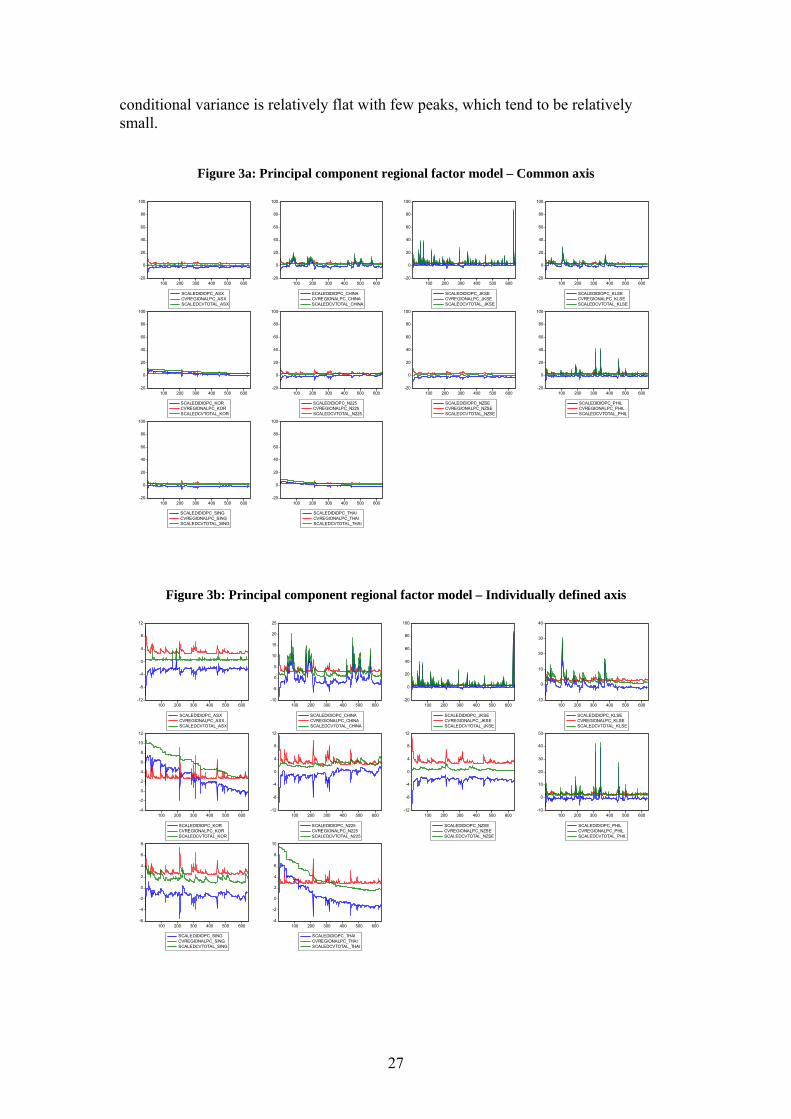
27
conditional variance is relatively flat with few peaks, which tend to be relatively small.
Figure 3a: Principal component regional factor model – Common axis
-20
0
20
40
60
80
100
100 200 300 400 500 600
SCALEDIDIOPC_ASXCVREGIONALPC_ASXSCALEDCVTOTAL_ASX
-20
0
20
40
60
80
100
100 200 300 400 500 600
SCALEDIDIOPC_CHINACVREGIONALPC_CHINASCALEDCVTOTAL_CHINA
-20
0
20
40
60
80
100
100 200 300 400 500 600
SCALEDIDIOPC_JKSECVREGIONALPC_JKSESCALEDCVTOTAL_JKSE
-20
0
20
40
60
80
100
100 200 300 400 500 600
SCALEDIDIOPC_KLSECVREGIONALPC_KLSESCALEDCVTOTAL_KLSE
-20
0
20
40
60
80
100
100 200 300 400 500 600
SCALEDIDIOPC_KORCVREGIONALPC_KORSCALEDCVTOTAL_KOR
-20
0
20
40
60
80
100
100 200 300 400 500 600
SCALEDIDIOPC_N225CVREGIONALPC_N225SCALEDCVTOTAL_N225
-20
0
20
40
60
80
100
100 200 300 400 500 600
SCALEDIDIOPC_NZSECVREGIONALPC_NZSESCALEDCVTOTAL_NZSE
-20
0
20
40
60
80
100
100 200 300 400 500 600
SCALEDIDIOPC_PHILCVREGIONALPC_PHILSCALEDCVTOTAL_PHIL
-20
0
20
40
60
80
100
100 200 300 400 500 600
SCALEDIDIOPC_SINGCVREGIONALPC_SINGSCALEDCVTOTAL_SING
-20
0
20
40
60
80
100
100 200 300 400 500 600
SCALEDIDIOPC_THAICVREGIONALPC_THAISCALEDCVTOTAL_THAI
Figure 3b: Principal component regional factor model – Individually defined axis
-12
-8
-4
0
4
8
12
100 200 300 400 500 600
SCALEDIDIOPC_ASXCVREGIONALPC_ASXSCALEDCVTOTAL_ASX
-10
-5
0
5
10
15
20
25
100 200 300 400 500 600
SCALEDIDIOPC_CHINACVREGIONALPC_CHINASCALEDCVTOTAL_CHINA
-20
0
20
40
60
80
100
100 200 300 400 500 600
SCALEDIDIOPC_JKSECVREGIONALPC_JKSESCALEDCVTOTAL_JKSE
-10
0
10
20
30
40
100 200 300 400 500 600
SCALEDIDIOPC_KLSECVREGIONALPC_KLSESCALEDCVTOTAL_KLSE
-4
-2
0
2
4
6
8
10
12
100 200 300 400 500 600
SCALEDIDIOPC_KORCVREGIONALPC_KORSCALEDCVTOTAL_KOR
-12
-8
-4
0
4
8
12
100 200 300 400 500 600
SCALEDIDIOPC_N225CVREGIONALPC_N225SCALEDCVTOTAL_N225
-12
-8
-4
0
4
8
12
100 200 300 400 500 600
SCALEDIDIOPC_NZSECVREGIONALPC_NZSESCALEDCVTOTAL_NZSE
-10
0
10
20
30
40
50
100 200 300 400 500 600
SCALEDIDIOPC_PHILCVREGIONALPC_PHILSCALEDCVTOTAL_PHIL
-6
-4
-2
0
2
4
6
8
100 200 300 400 500 600
SCALEDIDIOPC_SINGCVREGIONALPC_SINGSCALEDCVTOTAL_SING
-4
-2
0
2
4
6
8
10
100 200 300 400 500 600
SCALEDIDIOPC_THAICVREGIONALPC_THAISCALEDCVTOTAL_THAI

28
Figures 3a and 3b suggest that while the principal component conditional variances are similar to the market capitalisation estimates, there are at least three areas of differentiation. The principal component regional factors’ conditional variance series oscillates more than their market capitalisation weighted counterparts. Further, the decline in the idiosyncratic conditional variance series of Korea and Thailand is less smooth in the principal component models. Unlike in the market capitalisation models, the idiosyncratic conditional variance in the principal component models for each of these markets also ends the sample smaller than the regional conditional variance component. Finally, the Australia principal component idiosyncratic component has fewer variance spikes than its market capitalisation counterpart. 6. Regional or World Effects? The results outlined in Section 5 suggest that Asian equity markets, with the exception of China, react to common information. Attention is now turned to the type of common information that these markets react to. Specifically, do Asian equity markets react to regional or world information, or both? Alternatively, are Asian equity markets integrated with world equity markets or Asian equity markets. To this end, an additional factor is included in Equation 10. Equivalent consecutive US SP500 returns are included as an additional explanatory variable in both factor models for all markets. The consecutive US SP500 are taken as a proxy of the world factor, and are calculated as the differences between the logs of the closing prices of the SP500 for US trading days immediately prior to the dates when all Asian equity markets are open. Previous day US closing prices are used to calculate US returns as these are the closest equivalent to a true consecutive US return, as the US market trades while Asia is closed. The following equations are estimated
21,.
21,,,,
2,,
2,,,,,,,,,,,, ),0(~;
−− ++=
+++=
tiintininintin
tintitintusintjnininti NRRr
εψσςϕσ
σεεηβα
(12)
where i represents the market return being modelled (Australia, China, Indonesia, Japan, Korea, Malaysia, New Zealand, Philippines, Singapore, or Thailand), j represents the factor calculated from all markets except market I, and Rus,t represents the US return relevant to ri,t. The estimated parameters of these models are presented in Table 14.

29
Table 14: Estimated return and variance parameters for regional and US GARCH models32 Market Return Variance
C(1) Region US C ARCH(1) GARCH(1) Adj-R2 Wald Tests
Principal Component Weighted Australia 0 0.095 0.292 0 0.033 0.936 0.455 161.168
0.955 11.834 22.048 2.405 2.742 46.808 0
China 0.001 0.02 -0.032 0 0.17 0.822 -0.006 0.154 1.043 0.586 -0.904 4.399 6.928 40.769 0.695
Indonesia -0.001 0.511 -0.162 0 0.23 0.354 0.14 2.271 -0.593 10.458 -3.391 4.262 5.958 2.99 0.132
Malaysia 0 0.339 -0.026 0 0.125 0.858 0.112 0.125 0.8 11.847 -0.738 4.914 10.444 75.482 0.724
Korea 0 0.864 0.275 0 0 1 0.363 4.742 0.435 22.423 5.377 -3.158 1.73 1639.646 0.03
Japan -0.001 0.376 0.219 0 0.091 0.296 0.267 20.028
-1.409 13.276 5.736 2.367 2.607 1.063 0
New Zealand 0 0.154 0.141 0 0.043 0.945 0.234 14.279
0.215 11.003 8.476 1.552 4.432 68.613 0
Philippines -0.001 0.593 -0.141 0 0.565 0.104 0.189 2.323 -1.723 25.778 -4.786 11.952 7.564 2.461 0.128
Singapore 0 0.66 0.069 0 0.038 0.925 0.486 1.286 -0.007 25.1 2.475 3.591 3.046 54.178 0.257
Thailand 0 0.697 -0.113 0 -0.008 1.003 0.273 1.437 0.423 15.03 -2.168 1.702 -6.101 2940.612 0.231
Market Capitalisation Weighted
Australia 0 0.19 0.287 0 0.045 0.874 0.468 25.409
1.273 11.466 22.776 2.112 2.701 18.954 0
China 0.001 0.033 -0.031 0 0.17 0.822 -0.005 0.004 1.064 0.631 -0.97 4.363 6.902 40.53 0.952
Indonesia -0.001 0.263 0.15 0 0.25 0.063 0.042 0.005 -0.656 3.317 3.078 7.514 6.865 0.657 0.944
Malaysia 0.001 0.184 0.124 0 0.098 0.884 0.052 0.334 0.882 4.045 4.06 4.678 9.494 76.764 0.563
Korea 0.001 1.311 0.389 0 -0.001 1.003 0.34 1.481 1.278 18.058 8.284 -3.849 -1.217 999.546 0.224
Japan -0.001 2.208 0.198 0 -0.013 1.009 0.316 9.849
-1.367 13.193 6.381 -3.027 -3.027 269.234 0
New Zealand 0 0.127 0.192 0 0.04 0.943 0.206 3.025 0.423 5.632 12.564 1.721 3.649 53.209 0.083
Philippines -0.001 0.322 0.167 0 0.113 0.795 0.07 1.248 -1.042 5.577 4.84 5.479 7.183 30.476 0.264
Singapore 0.001 0.557 0.281 0 0.073 0.856 0.306 4.34 0.859 14.553 11.184 4.818 4.598 36.703 0.038
Thailand 0.001 0.446 0.238 0 -0.018 1.004 0.121 0.975 1.251 8.367 6.003 10.807 -33.167 1623.252 0.324
32 Z-statistics are provided in brackets, and estimated parameters that are significantly different from the zero at the 99% confidence level are in bold.

30
The market capitalisation results for Equation (12) are similar to those of Equation (10). The adjusted R-square is generally only marginally higher and the Wald test results presented in column 9 of Table 14 suggest that while the estimated US parameter is positive and significant for each market except China, the sum of the US and regional return parameters estimated from Equation (12) is insignificantly different to the regional return parameters estimated from Equation (10) for all markets except Australia, Japan and (at the 95% level) Singapore.33 The GARCH parameters estimated from Equations (10) and (12) are also very similar. These results suggest that the market capitalisation-weighted regional factor contains similar information to the US/World factor. The principal component results of Equation (12) are also similar to those of Equation (10). While the US factor coefficient is insignificant or negative for all ASEAN markets, the principal component GARCH parameters estimated from Equations (10) and (12) are similar for all markets, and the adjusted R-square for the principal component models from Equation (12) are similar to the comparable measures from Equation (10) for all markets except Australia. The Wald test results suggest that the US factor appears to provide additional information for Australia, Japan, New Zealand and, at the 5% confidence level, Korea. These results suggest that for Indonesia, Malaysia, Philippines, Thailand and, perhaps, Korea and Singapore, the US factor provides little information additional to that which is already contained in Japanese returns. The principal component-weighted regional factor appears to contain region-specific information, while the market capitalisation-weighted factor does not. Rather, the Japanese return dominated market capitalisation-weighted factor contains common world information, similar to that contained in US returns. Interestingly, these high frequency results are very similar to the lower frequency, monthly closed price return data results of Heaney and Hooper (1999).34 Heaney and Hooper (1999) also find that regional effects are found to significantly influence the contemporaneous monthly returns of Australia, Japan (negatively), Malaysia, Philippines, Singapore, and Thailand, while world effects influence Australia, Japan, Korea, New Zealand, and Singapore. Further, Heaney and Hooper (1999) find that while Australia, Japan and Singapore returns are significantly affected by both regional and world influences, world influences are much larger for Japan and larger for Australia, while regional influences are found to be much larger for Singapore. These results, obtained from monthly data, are almost identical to the daily results outlined above. Given the sample period examined, there is a concern that the results may be driven by the contagion effects present during the East Asian crisis. All observations between 1 January 1997 and 31 December 1998 are excluded and equation (10) is re-estimated
33 The Wald Tests test whether the sum of the estimated US and regional parameters outlined in Table 14 is insignificantly different from the estimated regional parameters outlined in Table 12. Bold denotes that the estimates are insignificantly different. 34 These results are also similar to those of Johnson and Soenen (2002), who use Geweke log likelihood measures of feedback and ten years of daily returns. Johnson and Soenen (2002) find that the equity market returns of Australia, New Zealand, and Singapore are highly integrated with those of Japan, while Indonesia, Philippines, and Thailand are not.

31
for ASEAN countries with principal component factors. These results are presented in Table 15.
Table 15: Estimated return and variance parameters – Excluding East Asian crisis Market Return Variance
C(1) Region C ARCH(1) GARCH(1) Adj-R2
Principal Component Weighted Indonesia 0 0.217 0 0.082 0.483 0.029
0.001 0.001 0 0.073 0.377
Malaysia 0 0.38 0 -0.043 1.006 0.153
0 0 0 0.002 0.002
Philippines -0.001 0.351 0 0.332 0.211 0.053
0.001 0 0 0.061 0.15
Singapore -0.001 0.634 0 0.185 0.702 0.458
0.001 0 0 0.042 0.072
Thailand 0.001 0.486 0 -0.001 1.009 0.23 0.001 0 0 0.006 0.003
Table 15 suggests that while the explanatory power of the Indonesia and Philippines models decrease, all ASEAN markets are still significantly influenced by the regional factor. The results of this analysis do not appear to be driven by the contagion effects present during the East Asian crisis. 7. Conclusion This analysis suggests four general conclusions. First, the method used to calculate Asian regional factors affects the quality of the estimate. Second, regional effects do not appear to depend on the time horizon of the analysis. Third, increased direct trade in financial assets may well increase equity market integration. Finally, Japanese returns are a poor proxy for the East Asian regional factor. These conclusions are considered in more detail. Correctly estimating the regional factor as containing information common to all markets affects the characteristics of the estimated regional factor. Calculating daily regional factors using closing prices, when markets do not close simultaneously, appears to cause autocorrelation and, perhaps, heteroskedasticity in addition to that caused by persistence in the arrival of information. Asian regional factors calculated using consecutive returns do not have significant autoregressive properties or ARCH parameters. Further, the weighting used to construct the regional factor also affects the relevance of the estimated regional factor for equity markets in East Asia. . This paper’s results, which are based on consecutive return measures of regional influence calculated at approximately daily frequencies, are almost identical to those of Heaney and Hooper (1999), who constructed regional factors using monthly returns. While Heaney and Hooper (1999) do not use consecutive returns, monthly close price data does not suffer the non-synchronicity problems that consecutive

32
returns seek to rectify. Consequently, the similarity between these results suggests that regional effects are not time horizon dependent, when market closures and the different time zones in which Asian equity markets trade are explicitly addressed. High frequency regional effects do not differ from the low frequency effects that have been estimated in previous work to as great a degree as previously thought. Previous results suggested that the positively autocorrelated regional factor had a small, often statistically insignificant, affect at daily frequencies, which accumulated through time, arising in a statistically significant regional influence at lower frequencies. This appears to be incorrect. The regional factor is not autocorrelated and when correctly measured, daily and monthly regional influences are approximately equal. But for China, regional effects are found to influence the returns of all East Asian equity markets, particularly those of Indonesia, Malaysia, Philippines, Singapore and Thailand. World effects are found to influence Australia, Japan, Korea, New Zealand and Singapore. While Australia and Singapore returns are significantly affected by both world and regional influences, regional influences are found to be much more important for Singapore. China is different from the other markets examined. China comprises stocks that can only be traded by Chinese nationals. It appears that regional information is largely irrelevant for this index. This conclusion is specific to the Shanghai A index. Chinese stocks listed in Hong Kong or Shanghai B stocks may be influenced by the common regional effect. The other less developed markets in Asia, particularly those of ASEAN countries, appear to have equity markets that are integrated with one another, but segmented from the world. This suggests that an increase in trade may well increase countries’ financial market integration and that restrictive trade blocs such as ASEAN lead to markets that are partially segmented from world markets, while integrated within the smaller group. Alternatively, it may suggest that ASEAN equity markets price from Singapore rather than Japan. Developed Asian equity markets appear to be integrated with each other, and the world, although not fully. This finding supports those of King, Sentana and Wadhwani (1994), Bekaert and Harvey (1995), Choi and Rajan (1997), and Heaney and Hooper (1999), which all suggest that even developed markets are not fully integrated with the world factor Finally, the results also suggest that Japanese returns are a poor proxy of the regional factor. They appear to represent world or US information more than regional information. Principal component-weighted regional factors appear a more appropriate measure of the Asian regional factor than either a market capitalisation-weighted regional factor or Japanese returns.

33
References Bekaert, G., and Harvey, C.R., 1995, Time-Varying World Market Integration, The Journal of Finance v50 n2, pp. 403-444 Bekaert, G., Harvey, C.R., and Lumsdaine, R.L., 2002, Dating the Integration of World Equity Markets, Journal of Financial Economics n65, pp.203-247 Choi, J.J., and Rajan, M., 1997, A Joint Test of Market Segmentation and Exchange Risk Factor in International Capital Markets, Journal of International Business Studies V28 n1, pp. 29-50 Fernandes, N., 2003, Market Integration and International Asset Allocation, IESE Business School Working Paper Forbes, K.J., and Chinn, M., 2003, A Decomposition of Global Linkages in Financial Markets Over Time, MIT-Sloan School of Management Working Paper Hamao, Y., Masulis, R.W., and Ng, V., 1990, Correlations in Price Changes and Volatility across International Stock Markets, The Review of Financial Studies v3 n2, pp. 281-307 Heaney, R., and Hooper, V., 1999, World, Regional and Political Risk Influences Upon Asia Pacific Equity Market Returns, Australian Journal of Management v24 n2, pp. 131 - 142 Johnson, R., and Soenen, L., 2002, Asian Economic Integration and Stock Market Comovement, The Journal of Financial Research v25 n1, pp. 141-157 Karolyi, G.A., and Stulz, R.M., 1996, Why Do Market Move Together? An Investigation of US-Japan Stock Return Comovements, The Journal of Finance v51 n3, pp.951-986 King, M., Sentana, E., and Wadhwani, S., 1994, Volatility and Links Between National Stock Markets, Econometrica v62 n4, pp. 901-933 Moshirian, F., 1998, The Asia-Pacific Financial Axis: Challenges for Further Financial Integration, Journal of Multinational Financial Management v8, pp. 103-112 Ng, A., 2000, Volatility Spillover Effects From Japan and the US to the Pacific Basin, Journal of International Money and Finance v19, pp. 207-233 Working, H., 1960, Note on the Correlations of First Differences of Averages in a Random Chain, Econometrica v28 n4