region of interest based image classi cation: a...
TRANSCRIPT
Region Of Interest Based ImageClassification: A Study in MRI
Brain Scan Categorization
Thesis submitted in accordance with the requirements of
the University of Liverpool for the degree of Doctor in
Philosophy
by
Ashraf Elsayed
November 2011

2

Dedication
To my family,especially
my wife and my children
i

ii
Abstract
This thesis describes research work undertaken in the field of image mining. More
specifically, the research work is directed at image classification according to the
nature of a particular Region Of Interest (ROI) that appears across a given image
set. Four approaches are described in the context of the classification of medical
images. The first is founded on the extraction of a ROI signature using the
Hough transform, but using a polygonal approximation of the ROI boundary. The
second approach is founded on a weighted subgraph mining technique whereby
the ROI is represented using a quad-tree structure which allows the application
of a weighted subgraph mining technique to identify feature vectors representing
these ROIs; these can then be used as the foundation with which to build a
classifier. The third uses an efficient mechanism for determining Zernike moments
as a feature extractor, which are then translated into feature vectors to which a
classification process can be applied. The fourth is founded on a time series
analysis technique whereby the ROI is represented as a pseudo time series which
can then be used as the foundation for a Case Based Reasoner. The presented
evaluation is directed at MRI brain scan data where the classification is focused on
the corpus callosum, a distinctive ROI in such data. For evaluation purposes three
scenarios are considered: distinguishing between musicians and non-musicians,
left handedness and right handedness, and epilepsy patient screening.
iii

iv
Acknowledgement
First and Foremost, I am very grateful to my first supervisor Dr. Frans Coenen,
specially for his constant patience, ongoing support and encouragement through-
out the past four years. His enthusiasm, constructive criticism, research ideas
and always making time for discussions have made the completion of my Ph.D.
possible and highly enjoyable. I am privileged to have worked with him.
I would like to express my gratitude to my second supervisor, Dr. Marta
Garcıa-Finana, for her assistance, suggestions and valuable comments; and to
thank Dr. Vanessa Sluming, for her assistance and her medical expertise. I also
would like to express my gratitude to Joanne Powell for assistance in supplying
the “handedness” data set; and to my colleague, Chuntao Jiang (Geof), for our
collaborative research work.
The Department of Computer Science in general at the University of Liverpool
has been an excellent place in which to conduct research, and all members of staff
and colleagues have been encouraging and helpful whenever needed.
Fundamental to my being able to conduct this research was the financial sup-
port of the Egyptian government, so I also extend my gratitude to the Egyptian
Cultural Bureau in London, and Alexandria University.
Last, but by no means least, I am eternally indebted to my wife for her
constant support and encouragement, without whom the completion of my Ph.D.
would not have been possible to accomplish.
v

vi
Contents
Abstract iii
Acknowledgement v
List of Figures xi
List of Tables xiv
1 Introduction 1
1.1 Motivation . . . . . . . . . . . . . . . . . . . . . . . . . . . . . . . 2
1.2 Thesis Objectives . . . . . . . . . . . . . . . . . . . . . . . . . . . 4
1.3 Research Methodology . . . . . . . . . . . . . . . . . . . . . . . . 5
1.4 Contributions . . . . . . . . . . . . . . . . . . . . . . . . . . . . . 6
1.5 Thesis Organisation . . . . . . . . . . . . . . . . . . . . . . . . . . 7
1.6 Summary . . . . . . . . . . . . . . . . . . . . . . . . . . . . . . . 7
2 Background and Literature Review 9
2.1 Introduction . . . . . . . . . . . . . . . . . . . . . . . . . . . . . . 9
2.2 Magnetic Resonance Imaging (MRI) . . . . . . . . . . . . . . . . 10
2.3 Image Preprocessing, Registration and Segmentation . . . . . . . 11
2.3.1 MRI Segmentation Using Pixel Classification . . . . . . . . 14
2.3.2 MRI Segmentation Using Deformable Models . . . . . . . 15
2.3.3 MRI Segmentation Using Statistical Models . . . . . . . . 16
2.3.4 MRI Segmentation Using Fuzzy Based Approaches . . . . 16
2.3.5 MRI Segmentation Using Graph Based Approaches . . . . 17
2.4 Data Mining and Image Classification . . . . . . . . . . . . . . . . 17
2.4.1 Case Based Reasoning . . . . . . . . . . . . . . . . . . . . 20
2.4.2 Graph Mining . . . . . . . . . . . . . . . . . . . . . . . . . 22
vii

2.5 Image Representation . . . . . . . . . . . . . . . . . . . . . . . . . 24
2.5.1 Region Based Methods . . . . . . . . . . . . . . . . . . . . 25
2.5.2 Boundary Based Methods . . . . . . . . . . . . . . . . . . 33
2.6 Summary . . . . . . . . . . . . . . . . . . . . . . . . . . . . . . . 40
3 MRI Datasets: Preprocessing and Segmentation 43
3.1 Introduction . . . . . . . . . . . . . . . . . . . . . . . . . . . . . . 43
3.2 Application Domain . . . . . . . . . . . . . . . . . . . . . . . . . 44
3.3 Image Preprocessing and Registration . . . . . . . . . . . . . . . . 45
3.4 Brain MR Image Segmentation . . . . . . . . . . . . . . . . . . . 46
3.4.1 Normalized Cuts Criterion . . . . . . . . . . . . . . . . . . 48
3.4.2 Optimal Graph Partition Computation . . . . . . . . . . . 49
3.4.3 Multiscale Normalized Cuts . . . . . . . . . . . . . . . . . 51
3.4.4 Proposed Approach . . . . . . . . . . . . . . . . . . . . . . 55
3.5 Medical Image Datasets . . . . . . . . . . . . . . . . . . . . . . . 60
3.6 Summary . . . . . . . . . . . . . . . . . . . . . . . . . . . . . . . 61
4 Region Of Interest Image Classification Using a Hough Trans-
form Signature Representation 63
4.1 Introduction . . . . . . . . . . . . . . . . . . . . . . . . . . . . . . 63
4.2 The Straight Line Hough Transform . . . . . . . . . . . . . . . . . 65
4.3 Extensions of the Basic Hough Transform . . . . . . . . . . . . . . 67
4.3.1 Circles and Ellipses . . . . . . . . . . . . . . . . . . . . . . 67
4.3.2 Generalized Shapes . . . . . . . . . . . . . . . . . . . . . . 70
4.4 Proposed Image Classification Method . . . . . . . . . . . . . . . 72
4.4.1 Step 1: Preprocessing . . . . . . . . . . . . . . . . . . . . . 73
4.4.2 Step 2: Polygonal Approximation . . . . . . . . . . . . . . 74
4.4.3 Step 3: Shape Signature Extraction . . . . . . . . . . . . . 77
4.4.4 Classification . . . . . . . . . . . . . . . . . . . . . . . . . 78
4.5 Evaluation . . . . . . . . . . . . . . . . . . . . . . . . . . . . . . . 78
4.6 Discussion . . . . . . . . . . . . . . . . . . . . . . . . . . . . . . . 82
4.7 Summary . . . . . . . . . . . . . . . . . . . . . . . . . . . . . . . 83
viii
5 Region Of Interest Image Classification Using a Weighted Fre-
quent Subgraph Representation 85
5.1 Introduction . . . . . . . . . . . . . . . . . . . . . . . . . . . . . . 85
5.2 Image Decomposition . . . . . . . . . . . . . . . . . . . . . . . . . 87
5.3 Feature Extraction Using gSpan-ATW Algorithm . . . . . . . . . 89
5.3.1 Definitions . . . . . . . . . . . . . . . . . . . . . . . . . . . 89
5.3.2 Frequent Subgraph Mining . . . . . . . . . . . . . . . . . . 90
5.3.3 Weighted Frequent Subgraph Mining . . . . . . . . . . . . 92
5.4 Feature Selection and Classification . . . . . . . . . . . . . . . . . 95
5.5 Evaluation . . . . . . . . . . . . . . . . . . . . . . . . . . . . . . . 96
5.5.1 Musicians Study . . . . . . . . . . . . . . . . . . . . . . . 96
5.5.2 Handedness Study . . . . . . . . . . . . . . . . . . . . . . 99
5.5.3 Epilepsy Study . . . . . . . . . . . . . . . . . . . . . . . . 101
5.5.4 The Effect of Feature Selection . . . . . . . . . . . . . . . 104
5.5.5 Time Complexity of the Proposed Graph Based Image Clas-
sification Approach . . . . . . . . . . . . . . . . . . . . . . 106
5.6 Discussion . . . . . . . . . . . . . . . . . . . . . . . . . . . . . . . 108
5.7 Summary . . . . . . . . . . . . . . . . . . . . . . . . . . . . . . . 108
6 Region Of Interest Image Classification Using a Zernike Moment
Signature Representation 111
6.1 Introduction . . . . . . . . . . . . . . . . . . . . . . . . . . . . . . 111
6.2 Zernike Moments . . . . . . . . . . . . . . . . . . . . . . . . . . . 113
6.3 Calculation of Zernike moments in terms of Geometric Moments . 116
6.4 Fast Calculation of Geometric Moments . . . . . . . . . . . . . . 118
6.5 Fast Calculation of Zernike Moments . . . . . . . . . . . . . . . . 120
6.6 Feature Extraction Based on Zernike Moments . . . . . . . . . . . 120
6.7 Evaluation . . . . . . . . . . . . . . . . . . . . . . . . . . . . . . . 121
6.7.1 Experimental Studies on the Validity of the Proposed Method
of Zernike Moments Computation . . . . . . . . . . . . . . 121
6.7.2 Speed of Calculation of Zernike Moments According to the
Proposed Approach . . . . . . . . . . . . . . . . . . . . . . 122
6.7.3 Classification Performance . . . . . . . . . . . . . . . . . . 124
ix

6.7.4 Time Complexity of the Proposed Classification Approach
Based on Zernike Moments . . . . . . . . . . . . . . . . . . 127
6.8 Discussion and Summary . . . . . . . . . . . . . . . . . . . . . . . 127
7 Region Of Interest Image Classification Using a Time Series Rep-
resentation 129
7.1 Introduction . . . . . . . . . . . . . . . . . . . . . . . . . . . . . . 129
7.2 Proposed Image Signature Based on Pseudo Time Series . . . . . 130
7.2.1 ROI Intersection Time Series Generation (ROI Int.) . . . 130
7.2.2 Radial Distance Time Series Generation (Rad. Dist.) . . . 132
7.3 Similarity Measure Using Dynamic Time Warping . . . . . . . . . 132
7.4 Framework for Image Classification Based on Time Series Repre-
sentation . . . . . . . . . . . . . . . . . . . . . . . . . . . . . . . . 137
7.5 Evaluation . . . . . . . . . . . . . . . . . . . . . . . . . . . . . . . 138
7.6 Summary . . . . . . . . . . . . . . . . . . . . . . . . . . . . . . . 139
8 Conclusion 141
8.1 Summary . . . . . . . . . . . . . . . . . . . . . . . . . . . . . . . 141
8.2 Comparison of the Proposed Approaches . . . . . . . . . . . . . . 143
8.3 Statistical Comparison of the Proposed Image Classification Ap-
proaches . . . . . . . . . . . . . . . . . . . . . . . . . . . . . . . . 149
8.4 Main Findings and Contributions . . . . . . . . . . . . . . . . . . 152
8.5 Future Work . . . . . . . . . . . . . . . . . . . . . . . . . . . . . . 154
Bibliography 158
A Published Work 177
x
List of Figures
2.1 An example brain scan image. The three images show (from left
to right) sagittal, coronal and axial planes. A common point is
marked in each image. . . . . . . . . . . . . . . . . . . . . . . . . 11
2.2 Midsagital MRI brain scan slice showing the corpus callosum (high-
lighted in the right-hand image). . . . . . . . . . . . . . . . . . . . 12
2.3 An example of 5-Nearest Neighbour Classification. . . . . . . . . . 22
3.1 The location of the corpus callosum in a brain MR image. . . . . 45
3.2 A typical brain MRI scan, (a) before the registration (first row
scans), and (b) after the registration (second row scans). . . . . . 47
3.3 The results obtained by the multiscale normalized cuts algorithm,
(a-d) the original brain MRI scans, (e-h) the corpus callosum ob-
tained by the multiscale normalized cuts. . . . . . . . . . . . . . . 56
3.4 Histogram of the pixel greyscale values of the corpus callosum. . . 56
3.5 Probability plot of the corpus callosum pixel values. . . . . . . . . 58
3.6 Thresholding with various threshold intervals. . . . . . . . . . . . 58
3.7 The results obtained by the multiscale normalized cuts algorithm
and the proposed approach, (a-d) the original brain MRI scans,
(e-h) the corpus callosum obtained by the multiscale normalized
cuts, (i-l) the corpus callosum obtained by the proposed algorithm. 59
4.1 The 1-m and m-1 SLHT. . . . . . . . . . . . . . . . . . . . . . . . 68
4.2 1-m and m-1 Hough transforms for circle detection. . . . . . . . . 70
4.3 An example of generalized Hough transform for arbitrary shapes. 71
4.4 The framework of the proposed approach based on Hough transform. 73
4.5 Polygonal approximation of corpus callosum corresponding to ε =
0.9 and M = 17. . . . . . . . . . . . . . . . . . . . . . . . . . . . 76
xi
4.6 Polygonal approximation of corpus callosum corresponding to ε =
0.4 and M = 52. . . . . . . . . . . . . . . . . . . . . . . . . . . . 76
4.7 Run time complexity for the classification of different datasets. . . 82
5.1 Framework of graph based approach. . . . . . . . . . . . . . . . . 86
5.2 Hierarchical decomposition (tessellation) of the corpus callosum. . 88
5.3 Tree representation of the hierarchical decomposition given in Fig-
ure 5.2. . . . . . . . . . . . . . . . . . . . . . . . . . . . . . . . . . 88
5.4 An example of calculating weights by the ATW scheme. . . . . . . 94
5.5 Run time complexity of image classification using musician dataset. 106
5.6 Run time complexity of image classification using handedness dataset.107
5.7 Run time complexity of image classification using Ep212 dataset. 107
6.1 (a) Digital image, (b) Mapping the digital image onto the unit circle.115
6.2 (a) Digital image, (b) Mapping the digital image into the unit circle.116
6.3 128× 128 Artificial binary test image. . . . . . . . . . . . . . . . . 123
6.4 CPU elapsed time(s) of the 128 × 128 binary test image for Wee
[150] and the proposed method. . . . . . . . . . . . . . . . . . . . 123
6.5 Run time complexity of image classification using different MRI
datasets. . . . . . . . . . . . . . . . . . . . . . . . . . . . . . . . . 128
7.1 ROI signature using the ROI Int. method. . . . . . . . . . . . . . 130
7.2 Conversion of corpus callosum into time series using the ROI Int.
method. . . . . . . . . . . . . . . . . . . . . . . . . . . . . . . . . 131
7.3 ROI signature using the Rad. Dist. method . . . . . . . . . . . . 132
7.4 An example of the alignment of two time series using DTW, (D
matrix and the warping path). . . . . . . . . . . . . . . . . . . . . 135
7.5 Global warping path constraints: (a) Sakoe-Chiba band, and (b)Itakura
parallelogram. . . . . . . . . . . . . . . . . . . . . . . . . . . . . 136
7.6 Run time complexity for the classification of different datasets. . . 139
8.1 Run time complexity for the classification of the musician dataset
using the four proposed ROIBIC approaches. . . . . . . . . . . . . 146
8.2 Run time complexity for the classification of the handedness dataset
using the four proposed ROIBIC approaches. . . . . . . . . . . . . 146
xii

8.3 Run time complexity for the classification of the epilepsy dataset
(Ep212) using the four proposed ROIBIC approaches. . . . . . . . 148
8.4 An example of ROC curve. . . . . . . . . . . . . . . . . . . . . . . 149
8.5 AR comparison between the proposed image classification approaches.151
xiii

xiv
List of Tables
4.1 TCV classification results for musicians study . . . . . . . . . . . 79
4.2 TCV classification results for handedness study . . . . . . . . . . 79
4.3 TCV classification results for Ep106 . . . . . . . . . . . . . . . . . 80
4.4 TCV classification results for Ep159 . . . . . . . . . . . . . . . . . 81
4.5 TCV classification results for Ep212 . . . . . . . . . . . . . . . . . 81
5.1 Notation used throughout this chapter. . . . . . . . . . . . . . . . 90
5.2 TCV classification results for QT-D4 data of musician study. . . . 97
5.3 TCV classification results for QT-D5 data of musician study. . . . 98
5.4 TCV classification results for QT-D6 data of musician study. . . . 98
5.5 TCV classification results for QT-D7 data of musician study. . . . 98
5.6 TCV classification results for QT-D4 data of handedness study. . 99
5.7 TCV classification results for QT-D5 data of handedness study. . 100
5.8 TCV classification results for QT-D6 data of handedness study. . 100
5.9 TCV classification results for QT-D7 data of handedness study. . 101
5.10 TCV classification results for QT-D4 data of Ep106. . . . . . . . . 101
5.11 TCV classification results for QT-D5 data of Ep106. . . . . . . . . 102
5.12 TCV classification results for QT-D6 data of Ep106. . . . . . . . . 102
5.13 TCV classification results for QT-D7 data of Ep106. . . . . . . . . 102
5.14 TCV classification results for QT-D4 data of Ep159. . . . . . . . . 103
5.15 TCV classification results for QT-D5 data of Ep159. . . . . . . . . 103
5.16 TCV classification results for QT-D6 data of Ep159. . . . . . . . . 103
5.17 TCV classification results for QT-D7 data of Ep159. . . . . . . . . 104
5.18 TCV classification results for QT-D4 data of Ep212. . . . . . . . . 104
5.19 TCV classification results for QT-D5 data of Ep212. . . . . . . . . 105
5.20 TCV classification results for QT-D6 data of Ep212. . . . . . . . . 105
5.21 TCV classification results for QT-D7 data of Ep212. . . . . . . . . 105
xv
5.22 The effect of feature selection for different datasets. . . . . . . . . 106
6.1 Comparison of theoretical ZTheopq , proposed Zprop
pq , and approxi-
mated Zapproxpq for f(xi, yj) = 1. . . . . . . . . . . . . . . . . . . . 122
6.2 TCV classification results for musicians study. . . . . . . . . . . . 125
6.3 TCV classification results for handedness study. . . . . . . . . . . 125
6.4 TCV classification results for Ep106. . . . . . . . . . . . . . . . . . 126
6.5 TCV classification results for Ep159. . . . . . . . . . . . . . . . . . 126
6.6 TCV classification results for Ep212. . . . . . . . . . . . . . . . . . 127
7.1 TCV classification results of different datasets. . . . . . . . . . . . 138
8.1 TCV classification results of different approaches for musicians study.145
8.2 TCV classification results of different approaches for handedness
study. . . . . . . . . . . . . . . . . . . . . . . . . . . . . . . . . . 145
8.3 TCV classification results of different approaches for epilepsy study
(Ep212). . . . . . . . . . . . . . . . . . . . . . . . . . . . . . . . . 145
8.4 Area Under the receiver operating characteristic Curve (AUC) re-
sults. . . . . . . . . . . . . . . . . . . . . . . . . . . . . . . . . . . 150
xvi
Chapter 1
Introduction
“Knowledge Discovery in Data (KDD) is the non-trivial process of identifying
valid, novel, potentially useful, and ultimately understandable patterns in data”
[49]. Data mining is an essential element within this process that is concerned
with the discovery of the desired hidden information within the data. The data
that data miners wish to mine comes in many different forms including: images,
graphs, text and so on. Consequently, data mining includes sub-fields such as
image mining, graph mining, and text mining. The work described in this thesis
is concerned with image mining.
Image mining is directed at the extraction of useful knowledge and relation-
ships from within image sets. Large amounts of visual information, in the form
of digital images, are generated on a daily basis with respect to many domains
such as the remote sensing and medical domains. Extracting useful knowledge
from within these images presents a significant challenge. Image mining also en-
compasses elements from fields such as image analysis and content based image
retrieval.
The work described in this thesis is directed at image classification, as opposed
to (say) image clustering. Image classification is a non-trivial problem, because
of the typically complex structure of image data, and is still a very active field of
research. In image classification, a collection of pre-classified (training) images are
taken as input and used to construct (train) a classifier which can then be applied
to unlabelled images. Image classification typically involves the pre-processing of
collections of images into a format whereby established classification techniques
may be applied. As with many data mining applications the main challenge in the
pre-processing of image data is to produce a representation whereby no relevant
1
information is lost while at the same time ensuring that the end result is succinct
enough to allow for the application of effective data mining. In image mining this
challenge is more acute because it is usually not clear what can be thrown away.
In most cases it is not possible to pre-process the images in such a way that all
pixel data, and the spatial relationships between pixels, can be retained; some
decision regarding resolution needs to be made. One approach is to apply some
form of segmentation to identify “blobs” (objects) within the images and then
use these objects to form an attribute set.
Image classification can be conducted with respect to as much of the informa-
tion contained in the images as possible, or can be focused on a particular object
or objects (blob or blobs) that occur across the image set. In this thesis the latter
is referred to as a Region Of Interest (ROI) and consequently the term ROI Based
Image Classification (ROIBIC) is used to identify this type of image classification.
The advantage offered is that the remainder of the image can be ignored and thus
computational advantages gained. Consequently, the representation can be more
detailed. The work described in this thesis is directed at ROIBIC.
The rest of this introductory chapter is organised as follows. The motivation
for the work is presented in Section 1.1. The research objectives and associated
research issues are presented in Section 1.2. The research methodology used to
address the research issues, including the “criteria for success”, is presented in
Section 1.3. An overview of the rest of this thesis is then given in Section 1.5,
and a summary of this chapter in Section 1.6.
1.1 Motivation
From the above, the research described in this thesis is directed at image clas-
sification, more specifically ROIBIC. Image classification, in whatever form, has
many applications. However, an important focus for image mining research is with
respect to medical applications. Global investment in the use of medical imaging
technology, such as Computed Tomography (CT), Magnetic Resonance Imagery
(MRI), Nuclear Medicine (NM) and MR Spectroscopy (MRS), has grown rapidly
over the last decade. The quantity of medical image data that is being generated
is fast becoming overwhelming, while at the same time there is a requirement
for ever more sophisticated tools to assist in the analysis of this imagery. Con-
2
sequently, medical image mining is attracting significant attention from both the
commercial and the research communities.
Medical diagnosis is often founded on a categorization (classification) of med-
ical images according to the nature of a specific object contained within such im-
ages rather than the entire image. Often the distinguishing features that would
indicate a particular classification are difficult to observe even by trained clin-
icians. Therefore there is a necessity for content based image classification to
classify these types of images according to the nature of a ROI contained within
them. This is then the motivation for the work described in this thesis.
The principal challenge of ROIBIC is the capture of the features of interest
in such a way that relative spatial information is retained. Some popular feature
representations are directed at colour, texture and/or shape. Little work has been
done on techniques that maintain the relative structure of the features of inter-
est. The work described in this thesis is directed at medical image classification
according to a particular feature of interest that appears across the image set.
There are many medical studies [4, 27, 31, 34, 38, 61, 74, 98, 124, 128, 149, 151]
that demonstrate that the shape and the size of specific regions of interest play a
crucial role in the image classification process. One example (and the application
focus of the work described) is that the shape of the corpus callosum, a promi-
nent feature located in brain MRI scans, is influenced by neurological diseases
such as epilepsy and autism, and by special abilities (such as mathematical or
musical ability) [111, 132, 149]. Many studies have shown a correlation between
the progression of Alzheimers disease (AD) and the decrease of volume in brain
periventricular structures, such as the hippocampus and the amygdala [50, 147].
In [146], a voxel discriminant map classification method is described applied to
brain ventricles in order to distinguish between healthy controls and Alzheimers
disease (AD) patients based on the shape of brain ventricles. In [55] the clinical
research problem of classifying the identical monozygotic and non-identical dizy-
gotic twin pairs according to the shape and size of brain ventricles structures has
been addressed.
In summary the work described is motivated by a need for techniques that
can classify images according to the shape and relative size of features of interest
that occur across some medical image sets. As noted above, one example is the
3
classification of MRI brain scan data according to the nature of corpus callosum
which features across those MRI brain scan collections.
1.2 Thesis Objectives
Given the motivation presented in the previous section, this thesis is targeted at
an investigation of techniques to facilitate the analysis of medical images accord-
ing to a ROI that may feature across such data sets. More specifically, the work
described investigates techniques for classifying 2D MR images, extracted from
3D MRI brain volumes, according to the nature of a ROI within these scans. The
research question to be addressed is thus how best to process image collections so
that efficient and effective classification, according to some ROI contained across
the image set, can be achieved. The techniques investigated assume that some
appropriate ROI exists across the image set, thus the proposed techniques will
not be applicable to all image classification problems, but the techniques will
be applicable to the subset of problems where classification according to a ROI
makes sense.
The above research question encompasses a number of research issues.
1. The techniques derived should serve to maximize classification accuracy
while at the same time allowing for efficient processing (although efficient
processing can be viewed as a secondary requirement to accuracy).
2. To achieve the desired classification accuracy any proposed feature extrac-
tion (representation) method should capture the salient elements of the ROI
without knowing in advance what those salient elements might be. In other
words any proposed feature extraction method, whatever form this might
take, should retain as much relevant information as possible.
3. Not withstanding point 2 it is also desirable to conduct the classification in
reasonable time, there is thus a trade off between accuracy and efficiency
that must be addressed.
4. Not all potential representations are compatible with all available classifica-
tion paradigms, thus different representations may require the application
of different classification techniques.
4
1.3 Research Methodology
To address the above research objective and associated issues the adopted research
methodology was to investigate and evaluate a series of techniques that could
be applied to extract and process ROIs. Although there are a great variety
of potential techniques that can be adopted for ROI representation this thesis
focuses on four techniques as follows:
1. Tree representations: The representation of ROI in terms of quad-trees
coupled with the application of a weighted frequent subgraph mining tech-
nique to identify frequently occurring subgraphs which can then be used as
the input to a standard classification algorithm.
2. Time series representations: The representation of ROI as time series
coupled with the application of a Case Based Reasoning (CBR) process to
achieve the desired classification.
3. Hough Transform: The application of Hough transform methods to ROIs
so as to extract a “signature” that encapsulates the desired details of the
ROI which can then be used in conjunction with appropriate classification
algorithms.
4. Zernike Moments: The representation of ROIs using Zernike moments
so as to define a “signature”, as in the case of (3), that both encapsu-
lates details of the ROI and is compatible with appropriate classification
algorithms.
The first two were selected because they were two very distinct techniques that
have (to the best knowledge of the author) not been previously applied in the
context of ROIBIC for MRI brain scan data. The third and fourth options were
selected because, from the literature, the Hough transform and Zernike moments
have frequently been applied in the context of image classification.
To facilitate the above an appropriate segmentation technique was required
so as to isolate the desired ROI contained within a given input image collection.
The investigation therefore commenced with the consideration of the nature of
the segmentation techniques that might be required. This was then followed by
5
consideration of the above four selected representations. To evaluate the effec-
tiveness of each technique standard measures (classification accuracy, specificity,
sensitivity and runtime) were used to assess the performance of the resulting clas-
sification. The aim was to identify the best performing technique. To support
the evaluation a number of MRI brain scan data sets were used. In each case
the proposed ROIBIC was directed at the classification of MRI brain scan data
according to the nature of the corpus callosum (introduced above).
1.4 Contributions
The contributions of the research work presented in this thesis can be summarized
as follows:
(a) A variation of the multiscale normalized cuts algorithm to achieve the desired
segmentation and delineation of a ROI contained across an image data set.
(b) A novel approach to MR image classification based on the Hough transform
coupled with a polygonal approximation. The aim of the application of the
polygonal approximation to the ROI was to obtain a smooth curve over a min-
imum number of line segments describing the region boundary. The Hough
transform was then used to extract (1D) image signatures.
(c) An effective approach to MR image classification based on a quad tree repre-
sented hierarchical decomposition coupled with a weighted frequent subgraph
mining algorithm in order to identify frequently occurring subgraphs (sub-
trees) within the quad-tree representation. The identified frequent subtrees
were viewed as defining a feature space which could be used to represent the
image set.
(d) A novel mechanism to speed up the computation of exact Zernike Moments,
also based on a quad-tree decomposition, and the usage of the resulting exact
Zernike moments to define signatures for input to a classification system.
(e) An effective mechanism to describe ROIs in the form of a time series cou-
pled with the use dynamic time warping to determine the similarity between
images within the context of a CBR framework.
6
1.5 Thesis Organisation
The organisation of the rest of this thesis is as follows. Chapter 2 provides
an extensive literature review on medical image classification systems and also
discusses the challenges associated with 2D image segmentation to identify the
desired ROIs. Chapter 3 describes the nature of the MRI brain scan datasets
and the application domain used as the focus for the work described in this thesis
and to evaluate the proposed techniques. The necessary data preparation and
image pre-processing is also described in this chapter. The four techniques con-
sidered are then described in the following four chapters. Chapter 4 deals with
image classification techniques using the Hough transform. A variation of the
Hough transform that employs a polygonal approximation of the curves repre-
senting the regions of interest is proposed. Chapter 5 describes the tree based
approach to image classification and an associated weighted frequent subgraph
mining technique is used to identify frequently occurring “patterns”. Chapter 6
presents the Zernike moments based signature representation ROIBIC technique
and includes consideration of mechanisms for the fast computation of Zernike
moments to enhance the accuracy and efficiency of the technique. In Chapter 7
the image classification framework based on a time series representation is de-
scribed. The chapter includes discussion of a “dynamic time warping” similarity
matching mechanism. Finally, in Chapter 8, this dissertation is concluded with a
summary, presentation and discussion of the main findings, and some suggestions
for future work.
1.6 Summary
This chapter has provided the necessary context and background to the research
described in this thesis. In particular the motivation for the research and the
thesis objectives have been detailed. A literature review of the related previous
work, with respect to this thesis, is presented in the following chapter (Chapter
2).
7

8
Chapter 2
Background and LiteratureReview
2.1 Introduction
In this chapter a review of the background and previous work with respect to the
research described in this thesis is presented. The chapter starts, Section 2.2, with
a review of the MRI brain scan application domain. In Section 2.3 a brief review
is then presented concerning image preprocessing, a necessary precursor to any
image analysis process. Broadly the work described in this thesis falls within the
domain of data mining, and more specifically image mining. Section 2.4 therefore
introduced the concept of data mining and then goes on to consider, in more
detail, the sub-domains of image mining and image classification. In particular
the application of Case Based Reasoning (CBR) to the classification problem and
frequent subgraph mining are discussed, because these are two of the techniques
used (in part) to provide an answer to the research question central to this thesis
(how best to process image collections so that efficient and effective classification,
according to some ROI contained across the image set, can be achieved?).
One of the main issues associate with image classification is how best to
represent the image input set so that an appropriate image mining technique can
be applied. The nature of this representation is of course related to the nature of
the image mining techniques to be adopted. A review of various representation
techniques, that impact on the representations proposed in this thesis, is thus
given in Section 2.5. A chapter summary is presented in Section 2.6.
9
2.2 Magnetic Resonance Imaging (MRI)
Magnetic Resonance Imaging (MRI) came into prominence in the 1970s. MRI
is similar to Computerized Topography (CT) in that cross-sectional images are
produced of some object. MRI uses a strong magnetic field and radio waves
to produce high quality and detailed computerized images of the inside of some
object. MRI is based on the principle of Nuclear Magnetic Resonance (NMR),
a spectroscopic technique used by scientists to obtain microscopic chemical and
physical information about molecules. The first successful Nuclear Magnetic Res-
onance (NMR) experiments were conducted in 1946 independently by two scien-
tists, Felix Bloch and Edward Purcell, both of whom were awarded the Nobel
Prize in 1952. In 1977, Raymond Damadian discovered the basis for using MRI
as a tool for medical diagnosis and demonstrated the first MRI examination of a
human subject [32]. The technique was called MRI rather than Nuclear Magnetic
Resonance Imaging (NMRI) because of the negative connotations associated with
the word nuclear in the late 1970’s. MRI started out as a tomographic imaging
technique, that is it produced an image of the NMR signal in a thin slice through
the human body. Since then MRI has advanced beyond a tomographic imaging
technique to a 3D imaging technique.
MRI is commonly used to examine the spine, joints, abdomen, and pelvis.
A special kind of MRI exam, called Magnetic Resonance Angiography (MRA)
can be used to examine blood vessels. MRI is also used for brain diagnosis, for
example to detect abnormal changes in different parts of the brain. A MRI of the
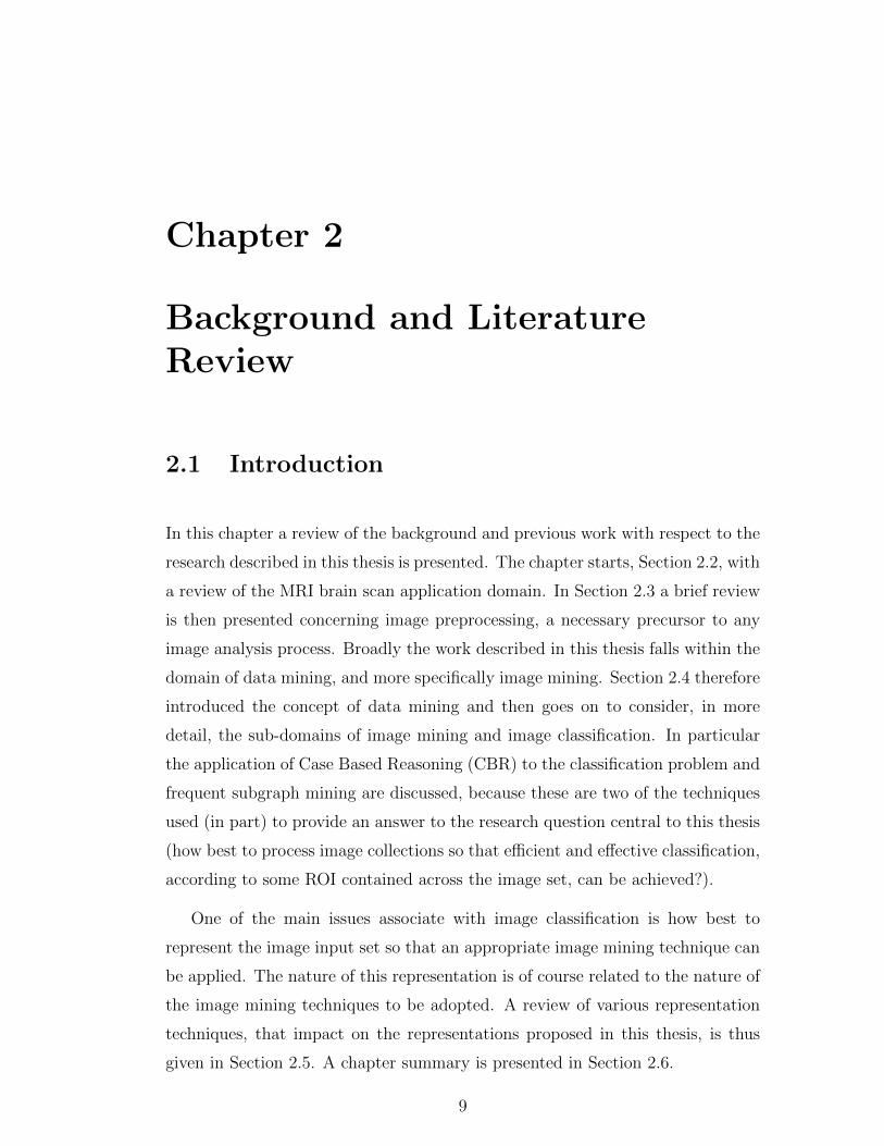
brain produces a very detailed picture. An example brain scan image is given in
Figure 2.1.
As noted in the previous chapter the focus of the work described in this
thesis is directed at the classification/categorisation of MRI brain scans according
to a particular feature (ROI) within these scans, namely the corpus callosum.
MRI brain scans underpin the diagnosis and management of patients suffering
from various neurological and psychiatric conditions. Analysis of MRI data relies
on the expertise of specialists (radiologists) and is therefore subjective. More
specifically the focus of the work is the classification of MRI brain scan data
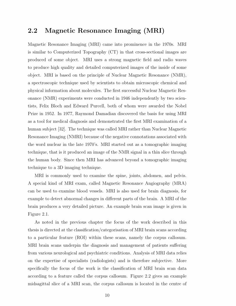
according to a feature called the corpus callosum. Figure 2.2 gives an example
midsagittal slice of a MRI scan, the corpus callosum is located in the centre of
10
Figure 2.1: An example brain scan image. The three images show (from leftto right) sagittal, coronal and axial planes. A common point is marked in eachimage.
the image. The midsagittal slice is the middle slice with a MRI scan, where a
MRI scan comprised a sequence (or bundle) of “image slices”.
The size and shape of the corpus callosum has been shown to be correlated
to sex, age, neurodegenerative diseases (e.g. epilepsy, multiple sclerosis and
schizophrenia) and various lateralized behaviour in people (such as handedness).
It is also conjectured that the size and shape of the corpus callosum reflects cer-
tain human characteristics (such as a mathematical or musical ability). Within
neuroimaging research considerable effort has been directed at quantifying pa-
rameters such as length, surface area and volume of structures in living adult
brains, and investigating differences in these parameters between sample groups.
Several studies indicate that the size and shape of the corpus callosum, in humans,
is correlated to sex [4, 34, 128], age [128, 151], brain growth and degeneration
[61, 98], handedness [31], epilepsy [27, 124, 149] and brain disfunction [38, 74]. It
is worth noting that although the work described in this thesis is directed at MRI
brain scan classification there are other features in MRI brain scans to which the
techniques could be applied, such as the ventricles.
2.3 Image Preprocessing, Registration and Seg-
mentation
The automated analysis of images, regardless of the nature of this analysis, typi-
cally requires some form of image pre-processing. This may include simple noise
11
Figure 2.2: Midsagital MRI brain scan slice showing the corpus callosum (high-lighted in the right-hand image).
removal and “deblurring” of objects. More advanced image preprocessing may
require operations such as registration and segmentation.
Registration is the process where by one or more images are aligned with a
reference image. This is important so that a collection of images can be effectively
compared. Image registration is used in a range of application domains, such as
medical image analysis (e.g. diagnosis), neuroscience (e.g. brain mapping), com-
puter vision (e.g. stereo image matching for shape recovery), astrophysics (e.g.
the alignment of images from different frequencies), etc. Image registration in the
medical domain is particularly difficult when complex (e.g. nonlinear) geometric
transformations are required to relate the images, e.g. when registering images
of different human brains (multi-subject registration). Registration of medical
image data sets can be defined as the problem of identifying a set of geometric
transformations which map the coordinate system of one data set to that of the
others. In the context of the work described in this thesis, image registration was
undertaken to ensure that all brain MRI scans in a given collection conformed
to a single set of coordinate axes. Therefore, all scans in the study have been
aligned manually by trained physicians.
Image segmentation is defined as the partitioning of an image into non-
12
overlapping meaningful regions that are homogeneous with respect to some char-
acteristic such as intensity, colour or texture or by extracting one or more specific
objects in images such as medical structures. Ideally a segmentation method finds
the group of pixels that correspond to anatomical structures or regions of interest
in the image, usually this is done by distinguish objects or regions of interest (the
“foreground”) from everything else (the “background”). In the simplest cases
there are only two pixel types (foreground and background), consequently the
segmentation results in a binary image. Segmentation is often the first stage in
an image analysis process. Once the regions of interest are isolated from the rest
of the image, certain characterizing measurements can be made and these can be
used to (say) classify the regions.
Image segmentation has gone through many stages of development and refine-
ment over the last few decades [108]. However, any individual image segmentation
technique is not likely to achieve reliable results under all circumstances; there
is no all purpose “best” segmentation technique. Medical image segmentation is
a key task in many medical applications such as surgical planning, post-surgical
assessment and abnormality detection. Segmentation is used, for example: (i)
in the detection of organs such as the brain, heart, lungs or liver in MRI scans;
and (ii) to distinguish pathological tissues, such as tumours, from normal tis-
sue. The most basic attributes used to identify the ROI are image grey scale
level or brightness, but other properties such as texture can be used. Medical
images mostly contain complicated structures and precise segmentation is often
deemed necessary for clinical diagnosis. A lot of methods for automatic and semi-
automatic image segmentation fail to partition medical images precisely due to
poor image contrast, inhomogeneity and weak boundaries between regions. This
includes brain image segmentation. The segmentation of brain MRI scans is a
challenging problem that has received much attention [118, 154].
A variety of artifacts (noise) may appear in MRI data. Since the artifacts
change the appearance of the image they may also affect the performance of a
segmentation algorithm. The most significant artifacts in image segmentation are
intensity inhomogeneities and the partial volume effect. Intensity inhomogeneities
are not always visible to the human eye, but can nonetheless have negative influ-
ence on automatic segmentation. This may manifest itself by making intensities
13
in one part of the image brighter or darker than another part. It is often caused
by the Radio Frequency (RF) coils used in the MRI acquisition process. The
partial volume effect occurs when a pixel can not be accurately assigned to one
tissue type. This is because the intensity of the pixel originates from more than
one tissue. It occurs when one pixel covers a number of different tissue types and
the collective signal emitted from these tissue cells makes up the detected inten-
sity of the pixel. The partial volume effect is most apparent at edges between
different tissues (regions).
Many image segmentation techniques are used in the context of brain MRI
segmentation including pixel classification, deformable models, statistical models,
fuzzy based approaches and graph based approaches. Each is discussed in the
following sub-sections.
2.3.1 MRI Segmentation Using Pixel Classification
Pixel classification methods segment brain structures pixel by pixel based on spa-
tial and appearance information, which are represented by pixel features. These
pixel features can include pixel coordinates describing the location, as well as
intensity values of filtered versions of MRI data that describe the appearance
of the region of interest. In classification-based segmentation image pixels are
represented as points in a high-dimensional space, in which the coordinate axes
are defined by the feature values associated with the pixel (for example colour
intensity). To segment an unlabelled target image using supervised classification
techniques, first manually labelled example images are used to train a pixel clas-
sifier. This is done by first sampling pixels from the training images and mapping
them to the feature space. In the feature space a decision boundary is then found
that best separates the groups of pixels labelled as regions, from the pixels that
were labelled as background in the examples. Different types of classifiers use
different methods to derive this boundary from the training samples. After train-
ing, the classifier is applied to the unlabelled target pixels by mapping them into
the feature space, and labelling them according to the decision boundary. The
more pixel features that are used the better the classifier’s ability to model the
region’s appearance and location. However, it also tends to increase the complex-
ity of the decision boundary which increases the risk of over-training (where the
14
classifier is over tuned to a particular training set) causing errors when classifying
images that were not used for training. This risk can be decreased by increasing
the number of examples, constraining the complexity of the decision boundary,
or decreasing the number of features by ignoring those that are not considered
relevant to the classification accuracy. The most important differences between
brain structure segmentation methods based on pixel classification are the num-
ber and type of pixel features used. In Powell et al. [117] up to 100 features
were employed, including the intensities of pixels and their direct neighbours.
Morra et al. [104] segmented the hippocampus using thousands of features and
the AdaBoost ensemble classification method [53].
2.3.2 MRI Segmentation Using Deformable Models
Methods based on the deformable model paradigm, such as the active contour
model, also called snakes, delineate brain regions of interest by fitting a boundary
model to the image, which incorporates some form of global shape knowledge.
Using Snake and Level Sets the shape information is relatively weak, as these tech-
niques merely enforce smooth boundaries [11]. Statistical shape models enforce
stronger shape constraints and are therefore better equipped to deal with low-
contrast boundaries. These models are constructed by parametrizing the shapes
of manually labelled examples, and learning their mean shape and typical varia-
tions. Examples of shape models used for brain segmentation have been reported
in [71, 80]. The most important difference between these methods is the flexibility
of the parametrization. As a general rule, models with many degrees of freedom
can describe a complex boundary, but also require more labelled examples to
represent the potential shape variation. The initialization of the boundary of-
fers a way to incorporate spatial information in a deformable model. Deformable
models operate by minimizing a cost function that generally has several local
minima. This usually ensures that the final result is close to the initialization
and can therefore be used as a de-facto constraint on the spatial domain of the
segmentation.
15
2.3.3 MRI Segmentation Using Statistical Models
Methods based on the statistical model paradigm pay attention to spatially in-
trinsic characteristics. The most popular stochastic model is the Markov Random
Field (MRF) model [14]. The MRF model, and its variants, have been successfully
used for brain MRI segmentation [138]. Ruan et al. proposed a fuzzy Markovian
method for brain tissue segmentation from magnetic resonance images that cal-
culated a fuzzy membership value for each pixel to indicate the partial volume
degree [125].
In unsupervised statistical segmentation techniques the number of class labels
and the model parameters are assumed to be unknown. Hence, estimations of
model parameters and image labels (where each group of pixels characterizing a
region of interest can be represented as an image label) are required simultane-
ously. Since, the image label estimation depends upon the optimal set of parame-
ters, the segmentation problem can be viewed as an incomplete data problem. To
handle this problem, an iterative scheme, the Expectation-Maximization (EM)
algorithm, has been proposed [103]. Zhang et al. proposed a Hidden Markov
Random Field (HMRF) model to achieve brain MRI segmentation in the case
of unsupervised statistical techniques [169]. A new Bayesian method for auto-
matic segmentation of brain MRI was proposed in [99] where a variant of the
EM algorithm was used so as to make the whole procedure more computationally
efficient.
2.3.4 MRI Segmentation Using Fuzzy Based Approaches
Fuzzy based segmentation approaches are increasing popular because of recent
developments in fuzzy set theory, the development of various fuzzy set based
mathematical modelling techniques, and its successful application in computer
vision systems [139]. Ahmed et al. proposed a bias correction Fuzzy C-Means
(FCM) segmentation algorithm in which they incorporated a neighbourhood reg-
ularizer into the FCM objective function to allow labelling of a pixel to be influ-
enced by the labels in its immediate neighbourhood [3]. The algorithm is realized
by incorporating the spatial neighbourhood information into the standard FCM
algorithm and modifying the membership weighting of each cluster. Siyal et al.
presented a modified FCM algorithm formulated by modifying the objective func-
16
tion of the standard FCM and used a special spread method for the classification
of tissues [137]. Wang et al. proposed a modified FCM algorithm, called mFCM,
for brain MR image segmentation [148]. Aboulella et al. proposed a statisti-
cal feature extraction technique for diagnosis of breast cancer mammograms by
combining fuzzy image processing with rough set theory [65].
2.3.5 MRI Segmentation Using Graph Based Approaches
Recently, automatic segmentation of MR images of the developing new born brain
has been addressed [118] using graph clustering and parameter estimation for find-
ing the initial intensity distributions. Cocosco et al. [24] used sample selection
through minimum spanning trees for intensity-based classification. Shi and Ma-
lik [135] proposed the Normalized Cuts (NCut) algorithm for image segmentation
problems, which is based on Graph Theory. The NCut algorithm treats an im-
age pixel as a node of a graph, and considers segmentation in terms of a graph
partitioning problem. A variation of this technique is used in the context of the
work described later in this thesis. Chapter 3 gives more details of this image
segmentation technique.
Note that with respect to the work described in this thesis a necessary pre-cursor
for the desired classification is the identification (segmentation) of the corpus cal-
losum, although the precise nature of the adopted segmentation algorithm is not
significant as its is the relative performance of the proposed representations with
respect the classification task that is central to the investigation described in this
thesis.
2.4 Data Mining and Image Classification
Data Mining is broadly concerned with the identification of hidden patterns in
data. Data mining is part of a super process called Knowledge Discovery in
Databases (KDD) [47, 48, 64] and draws on the fields of statistics, machine learn-
ing, pattern recognition and database management. Data mining first came to
prominence in the early 1990s when advances in computing technology meant
that large quantities of data could be effectively collected and stored, and sub-
sequently analysed. However, we can trace the origins of data mining to much
earlier work on machine learning and statistics [18, 48, 49, 64]. Originally data
17
mining was directed at tabular data, for example the analysis of the contents of
super market baskets [2]. Subsequently data mining techniques have been ap-
plied to many forms of data: examples include text [17], web usage logs [168],
and graphs [72]. The work described in this thesis is directed at image mining.
Image mining deals with the extraction of implicit knowledge from image
collections, for example image relationships or patterns, that are not explicitly
stored in the image database. The main challenge of image mining is concerned
with mechanisms to translate low-level pixel representations into high-level image
objects that can be efficiently mined [69, 110, 114, 166, 167].
One branch of data mining, and that of interest with respect to the work de-
scribed here, is classification (also sometimes referred to as categorisation). Clas-
sification is concerned with software systems to generate a “classifier” which can
then be used to classify (categorise) new data. Typically a pre-labelled training
set is used to build the classifier. Thus, in the case of the corpus callosum ap-
plication; the training data will comprise a set of labelled images, (say) epilepsy
and non-epilepsy, from which a classifier can be generated. This classifier can
then be used to categorise new images. Thus the goal of image classification is
to build a model that will be able to predict accurately the class of new, unseen
images. There are various techniques that can be used to generate the desired
classifier, examples include decision trees [122], Support Vector Machines (SVMs)
[28], KNN [100] and Naive Bayes [95].
For the work described in this thesis, the popular C4.5 decision tree classifier
[122] and SVMs [28] were adopted in Chapters (see 5 and 6). A C4.5 decision
tree consists of internal nodes that specify tests on individual input variables
or attributes that split the data into smaller subsets, and a series of leaf nodes
assigning a class to each of the observations in the resulting segments. The C4.5
algorithm builds decision trees using the concept of information entropy [122].
The entropy of a sample S of classified observations is given by:
Entropy(S) = −p1 log2(p1)− p0 log2(p0), (2.1)
where p1(p0) are the proportions of the class values 1(0) in the sample S, respec-
tively. C4.5 examines the normalised information gain (entropy difference) that
results from choosing an attribute for splitting the data. The attribute with the
18
highest normalised information gain is the one used to make the decision. The
algorithm then recurs on the smaller subsets.
Support Vector Machines (SVMs) have proved to be a useful technique for
data classification. SVMs have provided improvements in the fields of handwrit-
ten digit recognition, object recognition and text categorization, among others.
SVMs try to map the original training data into a higher dimensional space by
a kernel function Φ. The aim is then to identify a linear separating hyper-plane,
with the maximal margin between negative and positive samples, in this higher
dimensional space. From the mathematical point of view, given a training set of
instance label pairs (xi, yi); i = 1 · · · l, where xi ∈ Rn and y ∈ {−1, 1}l, SVMs
search for a solution to the following optimization problem:
minw,b,ξ
1
2wTw + C
l∑i=1
ξi
subject to : yi(wTΦ(xi) + b) ≥ 1− ξi; ξi > 0 (2.2)
Here training vectors xi are mapped into the higher dimensional space by the
function Φ. C > 0 is the penalty parameter of the error term. Furthermore,
K(xi, xj) ≡ Φ(xi)TΦ(xj) is the kernel function. There are four basic kernel
functions: linear, polynomial, radial basis and sigmoid functions. SVMs are able
to deal with two-class problems, but there exists many strategies to allow SVMs
work with a larger number of categories.
The automatic categorization of medical images is a challenging task that can
be of importance when managing real data collections. More specifically, be-
cause of the increasing amount of medical image data available, locating relevant
information in an efficient way presents a particular challenge. Moreover, the ex-
traction of appropriate visual descriptors to reduce the gap between the semantic
interpretation and the visual content of medical images remains a research issue
[106].
There has been a substantial amount of work on the application of classifi-
cation techniques within the medical domain. For example, Antonie et al. [161]
distinguished mammography tumours from the normal mammography using a
medical image classification approach. Many successful techniques for automatic
categorization of medical images rely on the same kind of feature space descrip-
tors as more general methods for generic image classification. For example, Avni
19
et al. [7] have successfully applied a Bag-of-Features (BoF) approach to the clas-
sification of X-Ray images. Their method uses histograms of vector quantized
scale invariant features for automatic organ recognition. Their Scale Invariant
Feature Transform (SIFT) technique computes a 128-bin gradient histogram as
a description vector for each salient region [96]. They have also applied their
method to discriminate between healthy and pathologic cases on a set of chest
radiography images. SIFT descriptors and the BoF representation have also been
successfully applied to binary classification problems related to endomicroscopic
images, thus enabling users to discriminate between neoplastic and benign cases
with high accuracy [5]. Another tool for feature extraction in medical image
retrieval and classification is the Local Binary Patterns (LBP) descriptor [109].
This descriptor is based on a very simple idea to efficiently describe the local
texture pattern around a pixel. LBP comprises a binary code that is obtained
by thresholding a neighbourhood according to the grey value of its centre. The
effectiveness of LBP for radiographic images has been recently demonstrated by
Jeanne et al. [78], who have found significant performance improvement over
other common visual descriptors. In the context of MRI scan classification, Yang
et al. [157] proposed an automatic categorization of brain MRI scans based on
Independent Component Analysis (ICA) coupled with an SVM technique to dis-
criminate MRI scans among Alzheimer patients, mild cognitive impairment, and
control subjects using whole brain images. In [83], a hybrid approach combines
an SVM technique and Genetic Algorithm (GA) to classify tumour and normal
tissue of brain MRI scans based on wavelet descriptors.
2.4.1 Case Based Reasoning
Case-Based Reasoning (CBR) is a well established Artificial Intelligence (AI).
CBR operates by using a Case Base (CB) of previous cases to solve a new case.
Essentially the features of the new case are compared with the features of the
cases in the CB and the identified most similar cases are used to formulate a
solution to the new case. Thus the basic idea behind CBR is to solve a current
problem by reusing solutions that have been applied to similar problems in the
past. At the highest level of generality, the CBR cycle may be described by four
tasks [1]: (i) retrieve the most similar case or cases, (ii) reuse the information and
20
knowledge in the retrieved cases to solve the problem, (iii) generate a solution,
and (iv) retain in the CB the parts of this experience likely to be useful for
future problem solving. In order to do the retrieval, case representation and case
indexing techniques are required so that it is possible to retrieve cases using a
similarity computation. The retrieved cases are then reused to provide a possible
solution to the given problem and therefore, a case adaptation mechanism is also
required.
CBR is not normally thought of as a data mining technique. However, if we
think of a case base (CB) as comprising a set of examples each with an associated
label then CBR can be used for classification purposes. CBR style systems have
been applied successfully in the context of classification. For example Nearest-
Neighbour Classification (NNC) systems [100] can be characterised as a simple
CBR technique. As noted above the goal of classification is to predict the class
membership of given entities. The basic idea of NNC is to use information about
records (cases) for which the class membership is already known. In order to
classify a new record (case), its description has to be compared to the descrip-
tions of the known records. From an abstract point of view, each record can be
characterised as a point in some problem space defined by the properties used
to describe the record (see Figure 2.3). To predict the class of the new record
its nearest neighbours within the problem space is identified using some distance
metric. Finally, the information about the class membership of these nearest
neighbours is used to predict the class the new record. Either the class of the ac-
tual nearest neighbour may be used or a weighted voting system may be adopted
where k nearest neighbours have been identified. In the example shown in Fig-
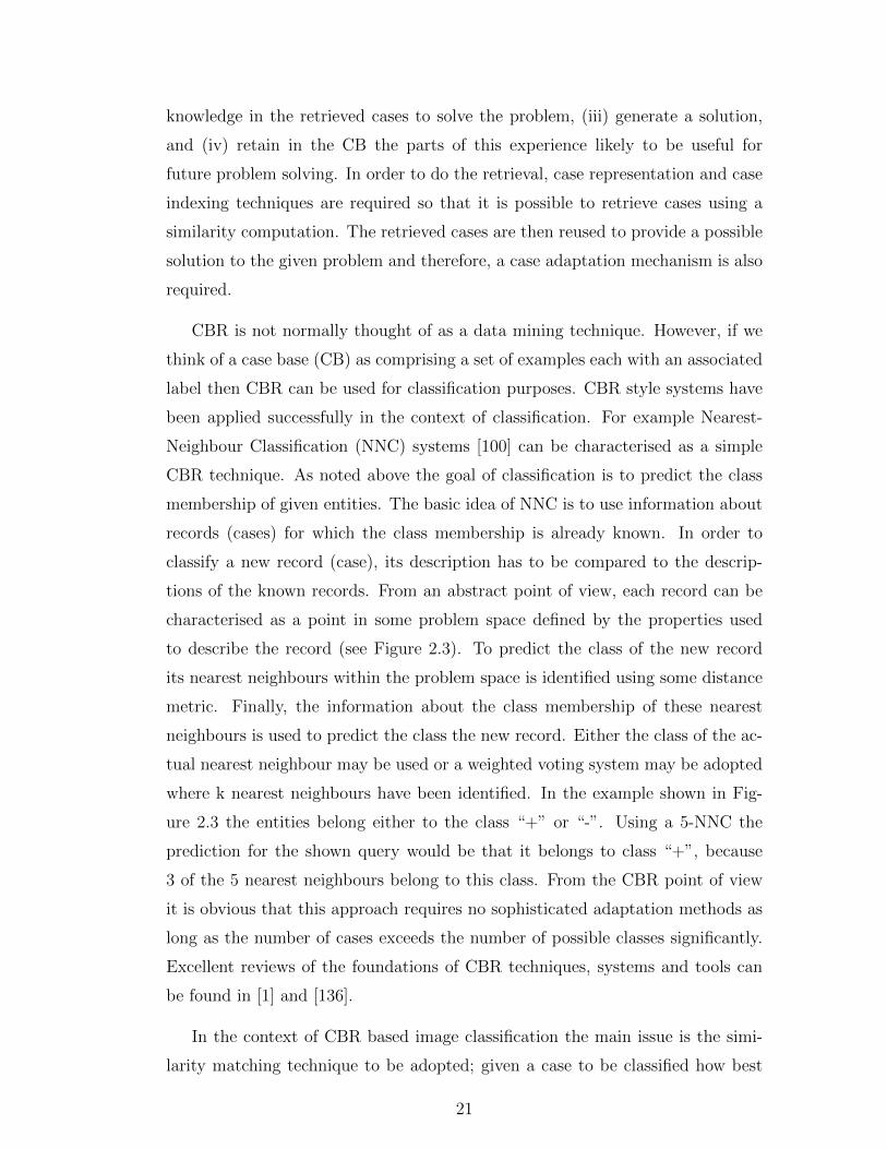
ure 2.3 the entities belong either to the class “+” or “-”. Using a 5-NNC the
prediction for the shown query would be that it belongs to class “+”, because
3 of the 5 nearest neighbours belong to this class. From the CBR point of view
it is obvious that this approach requires no sophisticated adaptation methods as
long as the number of cases exceeds the number of possible classes significantly.
Excellent reviews of the foundations of CBR techniques, systems and tools can
be found in [1] and [136].
In the context of CBR based image classification the main issue is the simi-
larity matching technique to be adopted; given a case to be classified how best
21
Figure 2.3: An example of 5-Nearest Neighbour Classification.
can this be matched with cases in the CB. The traditional measures used to com-
pare cases in CBR are distance measures (assuming of course that we are only
considering numerical attributes). Popular examples of such distance measures
are: Minkowsky distance, Hausdroff Distance, Bottleneck Distance and Reflection
Distance [143]. In the case of the work described here a Dynamic Time Warping
(DTW) technique has been adopted, this is described further in Chapter 7.
2.4.2 Graph Mining
Graph mining is the process of discovering hidden patterns (frequent subgraphs)
within graph datasets. From the literature graph mining can be categorized
in terms of transaction graph mining and single graph mining. In transaction
graph mining the dataset to be mined comprises a collection of small graphs
(transactions). The goal is to discover frequent recurring subgraphs across the
dataset. In single graph mining the input of the mining task is one single large
graph, and the objective is to find frequent subgraphs which occur within this
single graph. Frequent Subgraph Mining (FSM) has demonstrated its advantages
with respect to various tasks such as chemical compound analysis [73], document
image clustering [13], graph indexing [156], etc.
The straightforward idea behind FSM is to “grow” candidate subgraphs in
either a Breadth First Search (BFS) or Depth First Search (DFS) manner (can-
22
didate generation), and then determine if the identified candidate subgraphs occur
frequently enough in the graph data for them to be considered interesting (sup-
port counting). The two main research issues in FSM are thus how to efficiently
and effectively: (i) generate the candidate frequent subgraphs and (ii) determine
the frequency of occurrence of the generated subgraphs. Effective candidate sub-
graph generation requires that the generation of duplicate or superfluous candi-
dates is avoided. Occurrence counting requires repeated comparison of candidate
subgraphs with subgraphs in the input data, a process known as subgraph iso-
morphism checking. FSM, in many respects, can be viewed as an extension of
Frequent Itemset Mining (FIM) popularised in the context of Association Rule
Mining (ARM). Consequently, many of the proposed solutions to addressing the
main research issues effecting FSM are based on similar techniques found in the
domain of FIM.
It is widely accepted that FSM techniques can be divided into two categories:
(i) the Apriori-based approach (also called the BFS strategy based approach)
and (ii) the pattern growth approach. These two categories are similar in spirit
to counterparts found in ARM, namely the Apriori algorithm [2] and the FP-
growth algorithm [63] respectively. The Apriori-based approach proceeds in a
“generate-and-test” manner using a BFS strategy to explore the subgraph lattice
of the given database. Therefore, before exploring any (k+1)-subgraphs, all the k-
subgraphs should first be explored. For each discovered subgraph g, this approach
extends g recursively until all the frequent supergraphs of g are discovered [62].
Pattern growth approaches can use both BFS and DFS strategies, but the latter
is preferable to the former because it requires less memory usage.
One of the main challenges associate with FIM and FSM is the substantial
number of patterns which can be mined from the underlying database. This
problem is particularly important in the case of graphs since the size of the
output can be extremely large.
The significance of FSM with respect to the work described here is that one
of the techniques proposed uses this technique for the purpose of generating a
feature space. The application of FSM algorithms to the datasets described
in this work entails a significant computational overhead because of the great
number of generated frequent subgraphs. To reduce this overhead a Weighted
23
FSM approach can be applied, the objective being to focus on the identification
of those frequent subgraphs that are likely to be the most significant according
to some weighting scheme.
2.5 Image Representation
As noted above, image representation is an important issue with respect to image
classification. It is currently not computationally possible to present images to a
classification algorithm in their entirety, consequently it is necessary to process the
images in such a way that the classification process is tractable while at the same
time minimising information loss. Thus, one of the fundamental challenges of
image mining is to determine how the low-level pixel representation contained in a
raw image or image sequence can be efficiently and effectively processed to identify
high-level spatial ROIs and their relationships. Image classification techniques use
visual contents such as colour, texture, and shape to represent and classify images.
Colour and texture have been explored more thoroughly than shape. Because
shape is a more intrinsic property of ROIs than colour or texture, and given the
considerable evidence that natural ROIs are recognized based primarily on their
shape [107], the increasing interest in using the shape features of ROIs for image
classification is not surprising. The focus of this research is therefore on shape-
based image classification. Since humans can often recognize the characteristics
of ROIs using only their shapes, it is possible to expect shape-based techniques
to be intuitive as a tool for classifying images. However, image classification
by shape is still considered to be a more intrinsically difficult task compared to
image classification based on other visual features [107]. In addition, the problem
of shape-based image classification becomes more complex when the extracted
ROIs are corrupted by occlusions or noise as a result of the image segmentation
process.
Deriving shape descriptions is an important task in image classification. Once
the ROI has been acquired in the image, a set of techniques can be applied in
order to extract information from its shape, so that it can be analysed further.
This process is called shape description and generally results in a feature vector
(a shape descriptor). Shape description can be viewed as a mapping from a
shape space to a vector space that satisfies the requirement that two similar
24
shapes will also have close-to-identical shape descriptors while still allowing for
discrimination between different shapes. Note that it is not a requirement that
the original shape can be reconstructed from the feature vector. In most studies,
the terms shape representation and description are used interchangeably. Since
some of the representation methods are used as shape descriptors, there is no well-
defined separation between shape representation techniques and shape description
techniques. However, shape representation and description methods are defined in
[93] as follows. Shape representation results in non-numeric values of the original
shape. Shape description results in numeric values and is a step subsequent to
shape representation. For the sake of simplicity, we consider representation and
description to be synonymous and, throughout the rest of this section, collectively
refer to such techniques as shape description methods.
During the last decade, significant progress has been made with respect to
both the theoretical and practical aspects of shape description, and the litera-
ture reports a variety of techniques directed at describing ROIs based on their
shape. Two main approaches to deriving shape descriptors are region-based and
boundary-based (also known as the contour-based approach). In the region-based
approach, all the pixels defining a ROI are used in order to obtain the desired
shape descriptors (vectors). On the other hand, the boundary-based descriptor
approach uses only the boundary of a ROI to extract its shape descriptor. The
two approaches are considered in more detail in subsection 2.5.1 and 2.5.2 be-
low. The representations proposed in this thesis include both region based and
boundary based descriptions.
The problem of shape analysis has been pursued by many authors, thus,
resulting in a great amount of research. Recent review papers [93, 165] as well as
books [29, 41] provide a good overviews of the subject.
2.5.1 Region Based Methods
Region based shape descriptors express the pixel distribution within a 2D ROI.
They can be used to describe complex ROIs consisting of multiple disconnected
regions as well as simple ROIs with or without holes. Since it is based on the
regional property of a ROI, the descriptor is insensitive to noise that may be
introduced inevitably in the process of segmentation. From the literature we can
25
identify a number of techniques for generating region based shape descriptors,
examples include: (i) moments, (ii) simple scalar descriptors, (iii) angular radial
transformation descriptors, (iv) generic Fourier descriptors, (v) grid descriptors,
(vi) shape decomposition and (vii) medial axis transforms. A number of these
techniques form the foundation for some of the representations formulated later
in this thesis. Others have been included for consideration in this sub-section
purely for comparison purposes or because they are of historical interest.
2.5.1.1 Moments
Moments are widely used as shape descriptors. These moments can be classified
as being either orthogonal or non-orthogonal according to the basis used to derive
them. The most popular type of moments are called geometric moments which are
non-orthogonal moments that use a power basis (xp yq). The geometric moment
mpq of order p+ q of an (N ×M) digital image f(x, y) is defined as:
mpq =M−1∑x=0
N−1∑y=0
xpyqf(x, y) (2.3)
The use of moments for shape description was initiated in [70], where it was
proved that moment-based shape description is information preserving. The ze-
roth order moment m00 is equal to the shape area assuming that f(x, y) is a
silhouette function with value one within the shape and zero outside the shape.
First order moments can be used to compute the coordinates of the center of
mass as xc = m10/m00 and yc = m01/m00. Based on the moments formulated
in equation 2.3, a number of functions can be defined that are invariant under
certain transformations such as translation, scaling and rotation. The moment
invariants are then put into a feature vector. Global object features such as area,
circularity, eccentricity, compactness, major axis orientation, Euler number and
algebraic moments can all be used for shape description [120].
Central moments are constructed by subtracting the centroid from all the
coordinates. These moments are represented as:
µpq =M−1∑x=0
N−1∑y=0
(x− xc)p(y − yc)qf(x, y) (2.4)
The disadvantage of using these moments is that the basis used to derive these
moments is not orthogonal, so these moments suffer from a high degree of in-
26
formation redundancy. A generalization of moment transforms to other basis
is also possible by replacing a conventional basis xp yq by a form Pp(x)Pq(y),
for example orthogonal polynomials. In this case, the moments produce mini-
mal information redundancy, which is important for optimal utilization of the
information available in a given number of moments [93]. Some of the orthogonal
polynomial systems include Legendre and Zernike polynomials [141]. Teague [141]
adopt Zernike orthogonal polynomials to derive a set of invariant moments, called
Zernike moments. Zernike moments are defined as the projections of f(x, y) on
complex Zernike polynomials which form a complete orthogonal set over only the
interior of the unit circle; that is, x2 + y2 ≤ 1. The function of complex Zernike
moments with an order p and repetition q in polar coordinates is defined as:
ZMpq =p+ 1
π
∫ 2π
0
∫ 1
0
f(r, θ).V ∗pq(r, θ). r dr dθ (2.5)
Vpq(r, θ) is the Zernike polynomial, defined as:
Vpq(r, θ) = Rpq(r).eiqθ, i =
√−1 (2.6)
where p is a positive integer or zero and q is a positive integer subject to the
constraints that p− |q| is even and q ≤ p, r is the length of the vector from the
origin to the (x, y) pixel; i.e.,r =√x2 + y2, θ is the angle between the vector
r and the x axis in a counter-clockwise direction, the symbol (∗) denotes the
complex conjugate, and Rpq(r) is a real-valued Zernike-radial polynomial defined
as follows:
Rpq(r) =
p−|q|/2∑k=0
(−1)k.(p− k)!
k!(p+|q|
2− k)
!(p−|q|
2− k)
!.rp−2k (2.7)
Many researchers have adopted Zernike moments for many applications, such
as character recognition [15], face recognition [10], and shape retrieval [81]. Zernike
moment invariants have been shown to outperform several other shape descriptors
and to be highly effective in terms of image representation [85, 164]. Teh and Chin
[123] evaluated the performance of several moments with respect to issues such
as representation ability, noise sensitivity, and information redundancy. In terms
of overall performance, Teh and Chin showed that Zernike moments outperform
geometrical and Legendre moments. Further details about Zernike moments will
27
presented in Chapter 6 as this is the foundation of one of the representations
considered in this thesis.
2.5.1.2 Simple Scalar Descriptors
A shape can be described using scalar measures based on its simple geomet-
ric characteristics. These simple descriptors of a shape can often discriminate
only between shapes with large dissimilarities; therefore, they are usually used in
the context of image classification to act as filters to eliminate false hits or are
combined with other techniques to differentiate shapes. The advantage of these
descriptors is that they have a physical meaning. A brief description of the most
commonly used simple global descriptors is given below.
Eccentricity: Eccentricity (E) has been widely used as a scalar descriptor. It
illustrates the way in which the pixels of a ROI are scattered around the
centre of the ROI. E is defined as the ratio of the major axis of the ROI to
the minor axis. It is calculated using central moments such that [153]:
E =µ20 + µ02 +
õ2
20 + µ202 − 2µ02µ20 + 4µ2
11
µ20 + µ02 −√µ2
20 + µ202 − 2µ02µ20 + 4µ2
11
(2.8)
where µpq are the central moments of order (p+ q).
Solidity: Solidity (S) is computed as the ratio between the ROI area A0 and the
area of the corresponding convex hull. Solidity is computed as follows [153]:
S =A0
Convex Area(2.9)
Extent (Rectangularity): Extent (EX) is a measure that reflects the rectan-
gularity of a ROI [21], in other words, how much of a ROI fills its minimum
enclosing rectangle (MER). Extent is defined as:
EX =A0
AMER
(2.10)
where AMER is the area of the ROI’s MER.
Circularity (Compactness): Circularity (C) is a measure of roundness and is
defined as follows:
C =4π ∗ A0
(P0)2 (2.11)
28
where A0 is the ROI area, and P0 is the ROI perimeter.
It is sometimes used as inverse formula C = (P0)2
4π∗A0.
Euler’s Number: Euler’s Number is the difference between the number of con-
tiguous parts and the number of holes in the ROI.
Elongatedness: Elongatedness is the ratio between the length and width of the
region bounding rectangle.
2.5.1.3 Angular Radial Transform Descriptors
For region-based shape descriptions, the MPEG-7 working group has selected
angular radial transform descriptors [19] as MPEG-7 region based shape descrip-
tor. Angular radial transform (ART) descriptors are similar to Zernike moments
descriptors. The main difference is that ART descriptors are based on cosine
functions rather than on Zernike polynomials. The ART basis functions are sep-
arable along the angular and radial directions and are defined on the unit circle
as follows [19]:
Vpq(x, y) = Vpq(r, θ) =1
2πRp(r)e
iqθ (2.12)
The complex ART descriptors of order p with repetition q for a continuous
function f(x, y) are defined in polar coordinates as:
ARTpq =1
2π
∫ π
0
∫ 1
0
f(r, θ).Rp(r).e−iqθ r dr dθ (2.13)
where
Rp(r) =
{1 p = 02cos(pπr) p 6= 0
(2.14)
For a digital image, the integrals are replaced by summations to obtain:
ARTpq =1
2π
∑r
∑θ
f(rcosθ, rsinθ).Rp(r).e−iqθ r dr dθ , r ≤ 1 (2.15)
One of the advantages of the ART method is the compactness and efficiency in
describing the properties of multiple disjoint regions, simultaneously. It describes
the ROIs that may be split into disconnected sub-regions in the segmentation
process. It has been reported that Zernike moments outperform angular radial
transform descriptors in classifying ROIs that can be classified based on their
29
contours, but that ART descriptors perform better in the case of complex ROIs,
i.e., ROIs that consist of multiple contours, which can be classified only by region-
based techniques [101].
2.5.1.4 Generic Fourier Descriptors
A one-dimensional Fourier transform has been used successfully in image analysis
to derive shape descriptors from shape contours. Zhang and Lu [163] adopted
the 2D Fourier transform to derive a set of invariant descriptors called Generic
Fourier descriptors (GFD). In this method, the 2D ROI is transformed to the
polar coordinates, and the 2D Fourier transform is then applied in order to derive
shape descriptors. The rotation of the original ROI corresponds to a shift in the
normal Cartesian coordinates. This property makes it possible to derive rotation
invariant features by applying the 2D Fourier transform on the polar image and
then taking the magnitude while ignoring the phase. The 2D Fourier transform
of a polar image is give by [163]:
GFD(ρ, φ) =∑r
∑i
f(r, θi)e−j2π( rRρ+ 2πi
Tφ) (2.16)
where 0 ≤ r =√
(x− xc)2 + (y − yc)2 < R and θi = i(2π/T ), (0 ≤ i < T );
(xc, yc) is the center of mass of the ROI; 0 ≤ ρ < R, 0 ≤ φ < T . R and T are the
radial and angular resolutions.
The experiments conducted by Zhang and Lu [163] showed that GFD outper-
formed the use of ZM in retrieving ROIs based on the content of a region. Li
and Lee [91] proposed a technique which utilizes the magnitude of the Fourier
transform as well as phase coefficients in order to derive a set of invariant features.
2.5.1.5 Fourier-Mellin Descriptors
The Fourier-Mellin transform takes advantage of the properties of the Fourier
and Mellin transforms in order to define a new set of image invariants called
Fourier-Mellin Descriptors (FMDs). The Fourier-Mellin transform for f(r, θ) is
defined as follows [133]:
FMsl =1
2π
∫ π
−π
∫ ∞0
rs−1.f(r, θ).e−jlθ r dr dθ (2.17)
30
This transformation shows a radial-Mellin transform with parameter s and an
explicit circular-Fourier transform with parameter l [133]. The rotation invariant
can be achieved by taking the magnitude of the transform. Translation invariance
is conventionally achieved by placing the origin of the coordinates at the image
centroid.
Sheng and Duvernoy [133] employed the Mellin transform and the angular
Fourier complex componential factor to drive invariant Fourier-Mellin descrip-
tors. The problem associated with Fourier-Mellin descriptors is that the kernel
function of the Mellin transform is not orthogonal; hence, these invariants suf-
fer from a high degree of information redundancy. To overcome this problem,
Sheng and Shen [134] applied the Gram-Schmidt orthogonalization process to
orthogonalize the kernel function of the Mellin transform and used the resul-
tant orthogonal polynomial to derive a set of orthogonal Fourier-Mellin moments.
Their experiments demonstrated that, for small images, the description produced
by orthogonal Fourier-Mellin moments is better than that produced by Zernike
moments in terms of image-reconstruction errors and signal-to-noise ratio.
2.5.1.6 Grid Descriptors
The grid-based method has attracted interest because of its simplicity with re-
spect to representations [97]. In this technique, the given ROI is overlaid by a
grid space of a fixed size. A value of one is assigned to cells if they are at least
15% covered, and a zero is assigned to each of the other cells [97]. Then the 1s and
0s are scanned from left to right and top to bottom to obtain a binary sequence
for the ROI. It is also evident that the smaller the cell size, the more accurate
the representation of the ROI, but the greater the storage and computation re-
quirements. It is evident that the representation is translation invariant, but it
is not invariant to scale and rotation. Rotation and scale normalization are thus
necessary when grid descriptors are used to compare two ROIs. To achieve scale
normalization, all ROIs are scaled proportionally so that the major axes have the
same fixed length. For rotation invariance, the given ROI is rotated so that its
major axis is in parallel with the x-axis. The key problem associated with grid
descriptors is the problematic major axis normalization. The major axis is sensi-
tive to noise and can be unreliable even in the absence of noise effects. Moreover,
31
online classification usually involves extremely complex computations due to the
high degree of dimensionality of the feature vectors.
2.5.1.7 Shape Decomposition
This approach assumes that shape description is a hierarchical process and decom-
poses a ROI into a union of primitives that comprise the simplest elements which
form the region. Given the decomposition, a graph representation is constructed.
Syntactic pattern recognition techniques are, then, applied. Shape decomposition
methods generally use mathematical morphology. A morphological shape decom-
position technique is proposed in [116] where the binary ROIs are decomposed
into a union of simple regions. A structuring element (disk) is defined as the
simplest ROI component and the image is analysed as a union of the disks. The
representation is shown to be unique and invariant under rotation, translation
and scaling. Another morphological decomposition method, which is called Mor-
phological Signature Transform (MST) was developed in [94]. The MST method
utilizes multiresolution morphological image processing by multiple structuring
elements. The idea of this approach is to process decomposed, multiple shapes
instead of the original one. The decomposed shapes, called signature shapes,
contain substantial information about the whole shape. The method calculates
the area of the shape signatures obtained from multiple structuring elements and
multiple ROI scales to generate shape descriptors. Multiple structuring elements
are obtained by rotating single or multiple structuring elements. One of the ear-
liest types of shape decomposition of image data is the quad-tree [92]. It is a
tree-like representation of image data, where the image is recursively divided into
smaller regions. A quad-tree is a tree data structure in which each internal node
has exactly four children. The quad-tree decomposition is based on a recursive
subdivision of the image block into four quadrants according to the complexity
of the block. If a subimage is not a homogeneous block, it is subdivided into
four equal sized subimages again until all the subimages are homogeneous blocks.
A subimage is called a homogeneous block if the grey-level of each of the pixels
in the block is the same with respect to some specified constant. More details
concerning the quad-tree representation coupled with weighted frequent subgraph
mining is given in Chapter 5.
32
One of the problems in shape decomposition is the definition of the compo-
nents. The result of the decomposition does not always correspond to a human
intuitive shape representation. Furthermore, the results are not always unique.
The decomposition of similar shapes may result in different elements. In many
cases, the derivation of the decomposition is rather tedious and the computa-
tional complexity is relatively high compared to the other region based shape
description methods such as ART and moments.
2.5.1.8 Medial Axis Transform
The idea of the Medial Axis Transform (MAT) is to represent the shape by a
graph in which the important shape features are preserved [35]. The shape graph
is based on the region skeleton and the first step is the skeleton construction. The
skeleton is the set of all region points, which have the same minimum distance
from the region boundary for at least two separate boundary points. Generally,
MAT techniques use the region of the shape skeleton in order to derive shape
descriptors. The idea behind obtaining the skeleton of the region of a shape
is to preserve the topological information of the shape and to eliminate redun-
dant information. In other words, the skeletonization extracts a region-based
shape feature that represents the general form of a ROI. The shape’s skeleton
can be obtained by several techniques such as thinning algorithms, mathemati-
cal morphologic-based algorithms, and distance map-based algorithms [59]. After
skeletonization, the skeleton is decomposed into parts and represented as a graph.
Matching shapes then becomes a graph-matching problem. The difficulty with
skeleton-based techniques is that a small amount of noise or a variation in the
boundary often generates redundant skeleton branches that may seriously disturb
the topology of the skeleton’s graph [9]. Therefore, one of the weaknesses in the
medial axis transform is its sensitivity to noise in the shape boundary.
2.5.2 Boundary Based Methods
Boundary based shape description methods exploit only shape boundary informa-
tion. The shape properties of a ROI boundary are crucial to human perception in
judging shape similarity and recognition. Many authors who have studied the hu-
man visual perception systems, agree on the significance of high curvature points
33
of the shape boundary in visual perception [6]. In the psychological experiments,
it is suggested that corners have high information content and, for the purpose
of shape description, corners are used as points of high curvature. Therefore, the
shape boundary contains more information than the shape interior, in terms of
perception.
The previous sections have provided a review of several descriptors that are
based on the internal content of the shape. However, in many applications, the
internal content of the shape is not as important as its boundary. Boundary-
based techniques tend to be more efficient for handling shapes that are described
according to their contours [101]. From the literature we can identify a number
of techniques for generating boundary based shape descriptors, examples include:
(i) polygonal approximation, (ii) Hough transform, (iii) stochastic representation,
(iv) boundary approximation, (v) Fourier descriptors, (vi) coding, (vii) Curvature
Scale Space Descriptors and (viii) simple boundary descriptors. Each is discussed
in further detail below.
2.5.2.1 Polygon Approximation
Polygon approximation is one of the most popular shape representation methods,
where the continuous shape is represented by a set of vertices of a polygon [93].
The main idea is to eliminate the redundant and insignificant shape features by
reducing the number of boundary points. This is performed by searching the
break points on the boundary, based on an approximation criteria, such as mini-
mal error, minimal polygon perimeter or maximal internal polygon area. One of
the most widely used polygonal approximation algorithm is a heuristic method
called the Douglas-Peucker algorithm [37]. This iterative procedure repeatedly
splits the curve into smaller and smaller curves until the maximum of the per-
pendicular distances of the points on the curve from the line segment is smaller
than the error tolerance ε. In the approaches which use the split and merge algo-
rithm [113], where the curve is split into segments until some acceptable error is
reached, the split segments are merged if the resulting segment approximates the
curve within some maximum error. In [88] curve evolution is used as a polygonal
approximation method. Curve evolution reduces the influence of noise and sim-
plifies the shapes by removing the irrelevant features, keeping relevant ones. In
34
this method, a digital curve is regarded as a polygon, where each boundary point
is assumed to be a vertex, at the beginning of the evolution. In every evolution
step, a pair of consecutive line segments is substituted with a line segment, join-
ing the end points. The evolution process halts when the difference between the
evolved polygon and the original curve is higher than a given threshold. Curve
evolution methods assume that the shape boundary consists of various sources
of distortion, which should be removed by smoothing. The process of smoothing
depends on the predefined threshold value, which halts the evolution.
Corner detection is another approach for polygonal approximation. Popular tech-
niques for corner detection use Wavelet Transform Modulus Maxima (WTMM)
[121]. First, the shape boundary is represented by a 1D signal such as the con-
tour’s orientation profile. The singularities on that signal are then detected by
determining the local maxima of the wavelet transform of the signal.
2.5.2.2 Hough Transform
The Hough Transform (HT) is a widespread technique in image analysis. Its main
idea is to transform the image to a parameter space where clusters or particular
configurations identify instances of a shape under detection. HT based techniques
are used for shape detection, either parametrized or generalized. The HT was
first introduced by Paul Hough in 1962 [67] with the aim of detecting alignments
in T.V. lines. It became later the basis of a great number of image analysis
applications. The HT is mainly used to detect parametric shapes in images. It
was first used to detect straight lines and later extended to other parametric
models such as circles or ellipses, being finally generalized to any parametric
shape [12].
One major advantage offered by the HT is that it is highly robust against
image noise and degradation. The HT is used for extracting shape signatures
which can be used as a feature vector in the classification process. The HT is
suitable for this task because it maintains the spatial information associated with
an image ROI (feature). The “classic” HT performs a mapping between the X-
Y image space onto a ρ − θ space. The transformation is ρ = xcosθ + ysinθ,
where (x, y) are the coordinates of the pixel to be transformed, and (ρ, θ) are
the parameters of a corresponding line passing through the pixel. The parameter
35
space is suitably quantized into bins and represented by means of an accumulator
matrix initially set to zeros. Each pixel (x, y) can be conceptualised as a sinusoidal
(parametric) curve in the new ρ − θ space,where θ varies from the minimum
to the maximum values, giving the corresponding ρ values. The corresponding
sinusoidal positions can be stored in an accumulator matrix A, where each row
corresponds to one value of ρ, and each column to one value of θ. The cells in A
are then incremented by the parametric curve. The local maxima within A then
correspond to the dominant boundary lines of the ROI. Further details about the
HT are presented in Chapter 4.
2.5.2.3 Stochastic Representation
stochastic representation methods are based on the stochastic modelling of a
one dimensional function obtained from the shape boundary [93]. The idea is
to interpret the one dimensional function as a stochastic process realization and
use the model parameters obtained by estimation, as shape descriptors. For
example the Autoregressive (AR) model proposed in [82] to represent the closed
shape boundary. The one dimensional representation is obtained using a centroid
distance function. The AR model is, then, characterized by a set of unknown
parameters and an independent noise sequence. Given the function u(s), the
stochastic process is defined by:
u(s) = α +m∑j=1
θju(s− j) +√βωs (2.18)
where θj is the AR coefficients to be estimated, α is a constant to be estimated,√β is the variance of prediction noise and ωs is the independent random noise
source. θ1, ..., θm, α, β are called the model parameters. The shape descriptor vec-
tor is constructed using these parameters estimated by the Maximum Likelihood
Method. The same AR model is used in [39] with additional methods for improv-
ing classification performance. In [33], the AR model is extended to the bivariate
case and the classification results are further improved. The disadvantage of the
AR model is the sensitivity to shape occlusion [66]. The reason for this drawback
is that it models the whole shape with only one set of predictive parameters. If
the shape contains a large number of sample points and the contour varies rad-
ically, the shape may seem unpredictable. Therefore, an AR model with a finite
36
number of parameters is not adequate for the whole shape. In order to overcome
this drawback, the AR model is combined with the Hidden Markov Model in [66].
This approach segments closed shapes into segments, describes each segment by
AR modeling and finally analyzes the resulting vectors using a Hidden Markov
Model.
2.5.2.4 Boundary Approximation
Boundary approximation methods represent the curves by piecewise polynomial
interpolation, which results in a set of smooth curves inflected at control points.
Splines are used for the interpolation of functions to approximate shape segments.
The power of splines comes from the approximation of a given function with a
curve having the minimum average curvature. The main disadvantage of splines
is that the local function value modification changes the complete spline represen-
tation [93]. For this reason, B-splines are constructed so that the local function
value change does not spread to the rest of the intervals. Bsplines are piecewise
polynomial curves, whose shape is closely related to their control polygon which
is a chain of vertices giving a polynomial representation of a curve. If a control
polygon vertex changes its position, a resulting change of the spline curve oc-
cur only in a small neighbourhood of that vertex. In [25], curve representation
and matching is performed by B-splines. Another method, described in [26], use
splines for ROI modelling and shape estimation. Shape preserving approximation
based on splines is proposed in [68].
2.5.2.5 Fourier Descriptors
The Fourier representation decomposes a shape contour into its frequency com-
ponents (Fourier descriptors) obtained via its Fourier transform. The Fourier
transform is applied to the boundary function and the resulting coefficients are
used for shape description. For a given closed curve, which in turn is represented
by a one dimensional function u(s), the discrete Fourier transform is defined by:
an =1
N
N−1∑s=0
u(s)exp(−j2πns/N) (2.19)
The coefficients an, n = 0, 1, ..., N − 1, are used to derive Fourier descriptors.
In order to achieve translation and rotation invariance the phase information of
37
an is ignored and only the magnitude |an| is used. The magnitudes are divided
by the DC component |a0|, to achieve the scale invariance. In order to obtain
one dimensional function from the shape boundary, various methods have been
suggested such as tangent angle [160] and centroid distance [162]. The “classical
method” is to express the shape as a sequence of coordinates in the complex plane,
namely u(s) = x(s) + jy(s). Modified Fourier descriptors are used in [126] to
efficiently compute the feature matching. The Fourier descriptors represent global
information about the boundary. Therefore, local spatial information about the
shape is not readily available and the level of shape detail can only be controlled
on a global basis.
2.5.2.6 Coding
Coding methods describe a ROI by a sequence of unit size line segments with
a given orientation. One of the most popular coding scheme is Freeman’s chain
code [51], which is essentially obtained by mapping the shape boundary into a
2D parameter space, which is made up of codes. The chain code is defined as
the direction of the ROI’s contour from a starting point. This representation is
typically based on 4- or 8-connectivity, and the resulting chain code is a sequence
of numbers. There are many variations of Freeman chain codes. A generalized
chain code is proposed in [52], where the nodes surrounding a center node are
enumerated counter-clockwise in ascending order from inside out.
2.5.2.7 Curvature Scale Space Descriptors
Scale space representations are based on tracking the position of inflection points
in a boundary, filtered by low-pass Gaussian functions of variable widths [93]. The
inflection points, remaining in the representation are expected to be significant
object characteristics [93]. The Curvature Scale Space (CSS) approach proposed
in [102] is the most popular one in this class of methods. It has been selected as
the MPEG-7 contour based shape descriptor. Mathematically speaking, let Γ be
a closed planar curve and u be the normalized arc length parameter on Γ:
Γ = {(x(u), y(u)) |u ∈ [0, 1]} . (2.20)
38
In order to smooth the curve, functions x(u) and y(u) is convolved with a one
dimensional Gaussian kernel at different levels:
X(u, σ) = x(u) ∗ g(u, σ),
X(u, σ) = y(u) ∗ g(u, σ), (2.21)
g(u, σ) is a Gaussian kernel of width σ. The curvature of the smoothed curve is
then computed as:
k(u, σ) =X(u, σ)Y (u, σ)− X(u, σ)Y (u, σ)(
X2(u, σ) + Y 2(u, σ))3/2
, (2.22)
where X , Y and X , Y are the first and second derivatives of x(u, σ) and y(u, σ).
As σ increases, the shape of Γσ changes. This process of generating ordered
sequences of curves is referred to as the evolution of Γ. During evolution, the lo-
cations of curvature zero crossings of every Γσ is determined. The points are then
plotted in (u, σ) plane. The result of this process is represented as a binary image,
called a CSS image of the curve. Finally, shapes are described by the positions of
their CSS contour maxima. These positions projected onto the simplified object
contours give the positions of the mid points of the maximal convex/concave arcs,
obtained during the curve evolution. Since the small contours on the CSS image
represent some information about the existing noise on the actual object, those
maxima which are lower than a threshold are discarded. The shape similarity
measure between two shapes is computed by relating the positions of the max-
ima of the corresponding CSSs. The CSS image representation is invariant to
scale, rotation and translation. It is also robust to significant non-rigid deforma-
tions and perspective deformations. The basic drawback of this representation is
the difficulty in the determination of a threshold value in order to remove small
contours in CSS image. This process results in a decreased resolution, depending
on the predefined threshold value. Therefore, it requires procedures, which find
the necessary level of detail or use empirical parameters for sufficient resolution
of the shape contour.
2.5.2.8 Simple Boundary Descriptors
Boundary descriptors are mostly based on the geometric properties of the bound-
ary. Because of the discrete character of digital images, all of them are sensitive
39

to image resolution. In the following, popular geometric descriptors are provided
for the sake of completeness:
Bending Energy: Given a plane curve Γ = (x(u), y(u)) and its curvature func-
tion C(u) is given by:
C(u) =X(u)Y (u)− X(u)Y (u)(X2(u) + Y 2(u)
)3/2, (2.23)
where X , Y and X , Y are the first and second derivatives of x(u) and
y(u). The bending energy is defined as:
E =1
N
N∑u=1
C(u)2 (2.24)
Centroid Distance: The centroid distance function is expressed by the distance
of the boundary points from the centroid (xc, yc) of the ROI:
Dcentroid(s) =√
(x(s)− xc)2 + (y(s)− yc)2 (2.25)
Convexity(CX): A convex hull is the minimal covering of an ROI. A ROI con-
vexity can be defined as the ratio of perimeters of the convex hull to that
of the original contour (P0). The convexity is represented as [115]:
CX =Convex perimeter
P0
(2.26)
Aspect Ratio (AR): The aspect ratio is defined as the height of the ROI di-
vided by its width and is expressed as:
AR =Height of the ROI
Width of the ROI(2.27)
2.6 Summary
This chapter has presented the background and previous work with respect to
the research described in this thesis. Image classification, as a sub-domain of im-
age mining, and the challenges of medical image categorization were described.
In the context of image pre-processing prior to the application of image classi-
fication, several image segmentation techniques that may be applied to medical
40

images were introduced. A review of the literature concerned with ROIBIC was
presented. This review indicated that the number of types of shape descriptors
for image classification has been rapidly increasing over the last decade; however,
each technique has a number of shortcomings. In the next chapter the medical
brain MRI scan datasets that were used for the performance evaluation of the
proposed techniques are described. The process of preparing these images for
image classification, including image registration and image segmentation, will
also be presented.
41

42
Chapter 3
MRI Datasets: Preprocessingand Segmentation
3.1 Introduction
There have been major advances in the field of medical imaging over the past two
decades. New medical imaging technologies have provided physicians with pow-
erful, non-invasive techniques to analyse the structure, function, and pathology
of the human body. In more recent years the improvement in (and the devel-
opment of) many image acquisition techniques, the enhancement of the general
quality of the acquired images, advances in image processing and the develop-
ment of large computational capacities; have considerably enhanced the analysis
task. The acquisition of medical images in 2D or 3D has become a routine task
for clinical research applications. Image acquisition techniques include Magnetic
Resonance Imaging (MRI), Computed Tomography (CT), Positron Emission To-
mography (PET) and functional MRI (fMRI). The corresponding increase in the
quantity and detail of the available imagery has highlighted the need for more
efficient and more effective computer automated, or semi-automated, techniques
to support the interpretation of this data in order to provide better diagnosis and
treatment options.
The analysis of the increasingly detailed amount of information available con-
stitutes a great challenge for the medical imaging community, and requires sig-
nificant innovations in all aspect of image processing. One particular challenge
is related to the delineations of anatomical structures from medical images, this
is seen as a critical step for many clinical and research applications. As noted in
the introduction to this thesis the anatomical structure of interest is the corpus
43
callosum, a distinctive feature in MRI brain scans. Some background concerning
this application domain is therefore presented in Section 3.2.
The automated recognition of meaningful image components, anatomical struc-
tures, and other regions of interest, such as the corpus callosum, is typically
achieved using some kind of registration and segmentation techniques. Some
background concerning the registration of brain MRI scans is therefore consid-
ered in Section 3.3 as well as mechanisms to align collections of MRI scans to
some standard coordinates system. Some background concerning MRI brain scan
segmentation techniques is then presented in Section 3.4. In this section a vari-
ation of the Normalized Cut segmentation algorithm is proposed, an additional
contribution of this thesis, to identify the corpus callosum regions within brain
MRI scans. The section commences with some details concerning the original
“standard” normalized cuts algorithm, and the multiscale normalized cuts al-
gorithm. The latter was introduced to overcome the computational complexity
problem encountered when the standard normalized cuts algorithm is applied
to large images. Although, the multiscale normalized cuts produces good re-
sults with respect to many image segmentation applications it was found not
work efficiently with respect to the application domain considered in this thesis.
Therefore, a variation of the multiscale normalized cuts was proposed to deal
with this problem. This is fully described at the end of Section 3.4.
This chapter is concluded (Section 3.5) with some details concerning the image
data sets used for evaluation purposes with respect to the work described in the
reminder of this thesis.
3.2 Application Domain
MRI brain scans underpin the diagnosis and management of patients suffering
from various neurological and psychiatric conditions. Analysis of MRI data relies
on the expertise of specialists (radiologists) and is therefore subjective. The focus
of the research work described in this thesis is brain MR images, and in particular
a specific structure in these images called the corpus callosum which connects the
two hemispheres of the brain. Figure 3.1 gives an example of a brain MRI scan,
the corpus callosum is located in the centre of the image. The corpus callosum
was selected to evaluate the work described because it is of interest to medical
44
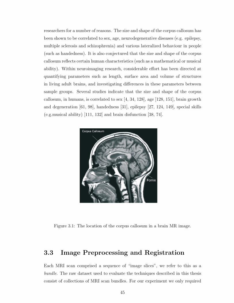
researchers for a number of reasons. The size and shape of the corpus callosum has
been shown to be correlated to sex, age, neurodegenerative diseases (e.g. epilepsy,
multiple sclerosis and schizophrenia) and various lateralized behaviour in people
(such as handedness). It is also conjectured that the size and shape of the corpus
callosum reflects certain human characteristics (such as a mathematical or musical
ability). Within neuroimaging research, considerable effort has been directed at
quantifying parameters such as length, surface area and volume of structures
in living adult brains, and investigating differences in these parameters between
sample groups. Several studies indicate that the size and shape of the corpus
callosum, in humans, is correlated to sex [4, 34, 128], age [128, 151], brain growth
and degeneration [61, 98], handedness [31], epilepsy [27, 124, 149], special skills
(e.g.musical ability) [111, 132] and brain disfunction [38, 74].
Figure 3.1: The location of the corpus callosum in a brain MR image.
3.3 Image Preprocessing and Registration
Each MRI scan comprised a sequence of “image slices”, we refer to this as a
bundle. The raw dataset used to evaluate the techniques described in this thesis
consist of collections of MRI scan bundles. For our experiment we only required
45
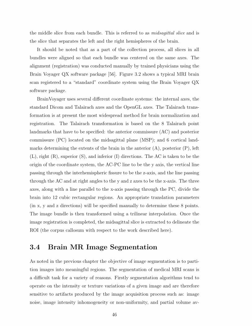
the middle slice from each bundle. This is referred to as midsagittal slice and is
the slice that separates the left and the right hemispheres of the brain.
It should be noted that as a part of the collection process, all slices in all
bundles were aligned so that each bundle was centered on the same axes. The
alignment (registration) was conducted manually by trained physicians using the
Brain Voyager QX software package [56]. Figure 3.2 shows a typical MRI brain
scan registered to a “standard” coordinate system using the Brain Voyager QX
software package.
BrainVoyager uses several different coordinate systems: the internal axes, the
standard Dicom and Talairach axes and the OpenGL axes. The Talairach trans-
formation is at present the most widespread method for brain normalization and
registration. The Talairach transformation is based on the 8 Talairach point
landmarks that have to be specified: the anterior commissure (AC) and posterior
commissure (PC) located on the midsagittal plane (MSP); and 6 cortical land-
marks determining the extents of the brain in the anterior (A), posterior (P), left
(L), right (R), superior (S), and inferior (I) directions. The AC is taken to be the
origin of the coordinate system, the AC-PC line to be the y axis, the vertical line
passing through the interhemispheric fissure to be the z-axis, and the line passing
through the AC and at right angles to the y and z axes to be the x-axis. The three
axes, along with a line parallel to the x-axis passing through the PC, divide the
brain into 12 cubic rectangular regions. An appropriate translation parameters
(in x, y and z directions) will be specified manually to determine these 8 points.
The image bundle is then transformed using a trilinear interpolation. Once the
image registration is completed, the midsagittal slice is extracted to delineate the
ROI (the corpus callosum with respect to the work described here).
3.4 Brain MR Image Segmentation
As noted in the previous chapter the objective of image segmentation is to parti-
tion images into meaningful regions. The segmentation of medical MRI scans is
a difficult task for a variety of reasons. Firstly segmentation algorithms tend to
operate on the intensity or texture variations of a given image and are therefore
sensitive to artifacts produced by the image acquisition process such as: image
noise, image intensity inhomogeneity or non-uniformity, and partial volume av-
46
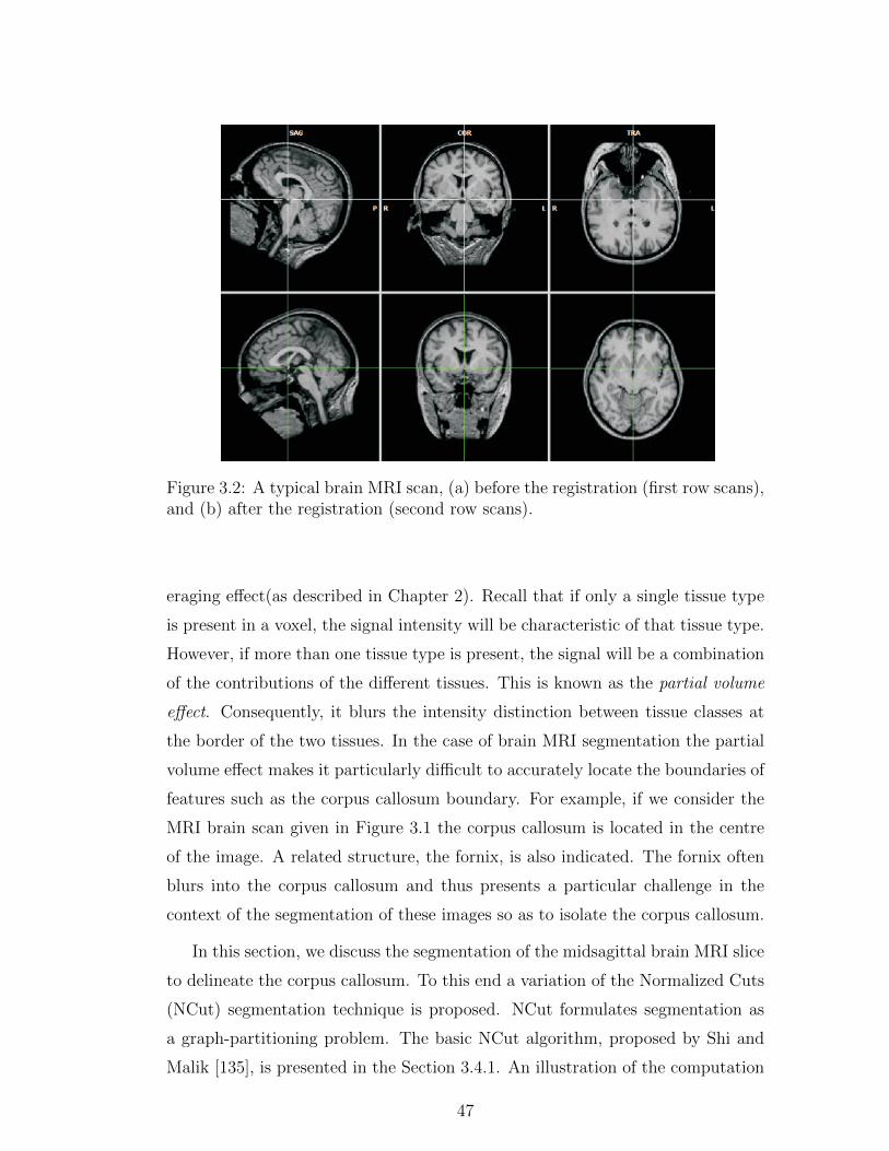
Figure 3.2: A typical brain MRI scan, (a) before the registration (first row scans),and (b) after the registration (second row scans).
eraging effect(as described in Chapter 2). Recall that if only a single tissue type
is present in a voxel, the signal intensity will be characteristic of that tissue type.
However, if more than one tissue type is present, the signal will be a combination
of the contributions of the different tissues. This is known as the partial volume
effect. Consequently, it blurs the intensity distinction between tissue classes at
the border of the two tissues. In the case of brain MRI segmentation the partial
volume effect makes it particularly difficult to accurately locate the boundaries of
features such as the corpus callosum boundary. For example, if we consider the
MRI brain scan given in Figure 3.1 the corpus callosum is located in the centre
of the image. A related structure, the fornix, is also indicated. The fornix often
blurs into the corpus callosum and thus presents a particular challenge in the
context of the segmentation of these images so as to isolate the corpus callosum.
In this section, we discuss the segmentation of the midsagittal brain MRI slice
to delineate the corpus callosum. To this end a variation of the Normalized Cuts
(NCut) segmentation technique is proposed. NCut formulates segmentation as
a graph-partitioning problem. The basic NCut algorithm, proposed by Shi and
Malik [135], is presented in the Section 3.4.1. An illustration of the computation
47
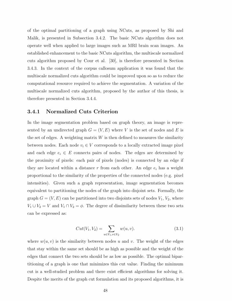
of the optimal partitioning of a graph using NCuts, as proposed by Shi and
Malik, is presented in Subsection 3.4.2. The basic NCuts algorithm does not
operate well when applied to large images such as MRI brain scan images. An
established enhancement to the basic NCuts algorithm, the multiscale normalized
cuts algorithm proposed by Cour et al. [30], is therefore presented in Section
3.4.3. In the context of the corpus callosum application it was found that the
multiscale normalized cuts algorithm could be improved upon so as to reduce the
computational resource required to achieve the segmentation. A variation of the
multiscale normalized cuts algorithm, proposed by the author of this thesis, is
therefore presented in Section 3.4.4.
3.4.1 Normalized Cuts Criterion
In the image segmentation problem based on graph theory, an image is repre-
sented by an undirected graph G = (V,E) where V is the set of nodes and E is
the set of edges. A weighting matrix W is then defined to measures the similarity
between nodes. Each node vi ∈ V corresponds to a locally extracted image pixel
and each edge ei ∈ E connects pairs of nodes. The edges are determined by
the proximity of pixels: each pair of pixels (nodes) is connected by an edge if
they are located within a distance r from each other. An edge ei has a weight
proportional to the similarity of the properties of the connected nodes (e.g. pixel
intensities). Given such a graph representation, image segmentation becomes
equivalent to partitioning the nodes of the graph into disjoint sets. Formally, the
graph G = (V,E) can be partitioned into two disjoints sets of nodes V1, V2, where
V1 ∪ V2 = V and V1 ∩ V2 = φ. The degree of dissimilarity between these two sets
can be expressed as:
Cut(V1, V2) =∑
u∈V1,v∈V2
w(u, v). (3.1)
where w(u, v) is the similarity between nodes u and v. The weight of the edges
that stay within the same set should be as high as possible and the weight of the
edges that connect the two sets should be as low as possible. The optimal bipar-
titioning of a graph is one that minimizes this cut value. Finding the minimum
cut is a well-studied problem and there exist efficient algorithms for solving it.
Despite the merits of the graph cut formulation and its proposed algorithms, it is
48
biased towards producing cuts that contain a small number of nodes. Therefore
Shi and Malik [135] proposed the normalized cuts algorithm (NCuts) as a new
measure of disassociation, the normalized cut (NCut) is defined as follows:
NCut(V1, V2) =cut(V1, V2)
SumCon(V1, V )+
cut(V1, V2)
SumCon(V2, V )(3.2)
where SumCon(V1, V ) is the total weights of the edges connecting nodes from a
set V1 to all nodes in the original set V and SumCon(V2, V ) is the total weights
of the edges connecting nodes from a set V2 to all nodes in the original set V . The
weight of the edges that stay within the same set are contained in SumCon(V1, V )
and SumCon(V2, V ), the weight of the edges that connect the two sets are con-
tained in cut(V1, V2). By minimizing this criterion the similarity across partitions
is minimized and the similarity within partitions is maximized simultaneously.
Unfortunately, minimizing this criterion constitutes an NP-complete problem but
Shi and Malik showed that when the normalized cut problem is embedded in a
real valued domain an approximate discrete solution can be found efficiently. The
details of solving this minimization problem is described in next section.
3.4.2 Optimal Graph Partition Computation
Shi and Malik [135] developed an efficient computational technique based on
a generalized eigenvalue problem to minimize the normalized cut. First, W is
defined as the affinity matrix of the graph which determines the connectivity of
the graph and defines the edges weights. Then the edges weights need to be
determined based on the similarity and distance between pixels. This is done by
applying the following formula for each edge:
wi,j =
{exp
−‖Ii−Ij‖2
σ2I· exp−‖Xi−Xj‖
2
σ2X
if ‖Xi −Xj‖ ≤ r
0 otherwise(3.3)
where: (i) wi,j is the weight of the edge that connects node i with node j, (ii) Ii
is the intensity of pixel i, (iii) Xi is the spatial location of pixel i, (iv) Ij is the
intensity of pixel j and (v) Xj the spatial location of pixel j. If there is no edge
between node i and node j then wi,j = 0 where the distance between node i and
node j is greater than distance r. The effect of this procedure is that the pixels
that are located very close to each other and that have a very small difference in
49
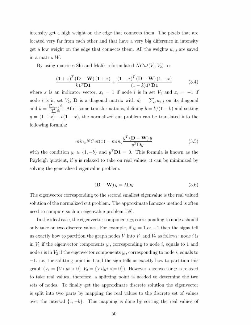
intensity get a high weight on the edge that connects them. The pixels that are
located very far from each other and that have a very big difference in intensity
get a low weight on the edge that connects them. All the weights wi,j are saved
in a matrix W .
By using matrices Shi and Malik reformulated NCut(V1, V2) to:
(1 + x)T (D−W) (1 + x)
k1TD1+
(1− x)T (D−W) (1− x)
(1− k)1TD1(3.4)
where x is an indicator vector, xi = 1 if node i is in set V1 and xi = −1 if
node i is in set V2, D is a diagonal matrix with di =∑
j wi,j on its diagonal
and k =∑xi=1 di∑i di
. After some transformations, defining b = k/(1− k) and setting
y = (1 + x) − b(1 − x), the normalized cut problem can be translated into the
following formula:
minxNCut(x) = minyyT (D−W) y
yTDy(3.5)
with the condition yi ∈ {1,−b} and yTD1 = 0. This formula is known as the
Rayleigh quotient, if y is relaxed to take on real values, it can be minimized by
solving the generalized eigenvalue problem:
(D−W) y = λDy (3.6)
The eigenvector corresponding to the second smallest eigenvalue is the real valued
solution of the normalized cut problem. The approximate Lanczos method is often
used to compute such an eigenvalue problem [58].
In the ideal case, the eigenvector components yi corresponding to node i should
only take on two discrete values. For example, if yi = 1 or −1 then the signs tell
us exactly how to partition the graph nodes V into V1 and V2 as follows: node i is
in V1 if the eigenvector components yi, corresponding to node i, equals to 1 and
node i is in V2 if the eigenvector components yi, corresponding to node i, equals to
−1. i.e. the splitting point is 0 and the sign tells us exactly how to partition this
graph (V1 = {V i|yi > 0}, V2 = {V i|yi <= 0}). However, eigenvector y is relaxed
to take real values, therefore, a splitting point is needed to determine the two
sets of nodes. To finally get the approximate discrete solution the eigenvector
is split into two parts by mapping the real values to the discrete set of values
over the interval {1,−b}. This mapping is done by sorting the real values of
50
this eigenvector and evaluating NCut(V1, V2) for a few evenly spaced splitting
points. The split point that produces the lowest NCut(V1, V2) will then finally
give us the approximate solution: the disjoint sets V1 and V2 together with their
NCut(V1, V2) value. The algorithm is recursively applied to every subgraph until
the value of NCut exceeds a certain threshold or the total number of nodes in
the partition is smaller than a pre-specified threshold value.
From the above, the procedure for image segmentation based on normalized
cuts can be summarized as follows:
1. Given an image I, construct an N × N symmetric similarity matrix W
according to Equation 3.3 and D as a diagonal matrix with di =∑
j wi,j on
its diagonal.
2. Solve the generalized eigenvalue problem
(D−W) y = λDy
and get the eigenvector with the second smallest eigenvalue.
3. Find the splitting point of eigenvector y, where yi ∈ {1,−b}, that minimizes
the NCut
4. Bipartition the graph nodes V into V1 and V2 according to this splitting
point.
5. Repeat the bipartition recursively, stop if the NCut value is larger than a
pre-specified threshold value or the total number of nodes in the partition
is smaller than a pre-specified threshold value.
The normalized cuts algorithm is computationally expensive when the dimen-
sion of the weight matrix is large because the pixel-based weight matrix required
to compute the N × N weight matrix becomes very dense. Consequently the
derivation of the eigenvalues becomes computationally expensive even though
the approximate eigenvalue method and associated algorithm are designed to
optimize this process.
3.4.3 Multiscale Normalized Cuts
Cour et al. [30] proposes a Normalized Cut adaptive technique, the Multiscale
Normalized Cuts algorithm, that focuses on the computational problem created
51
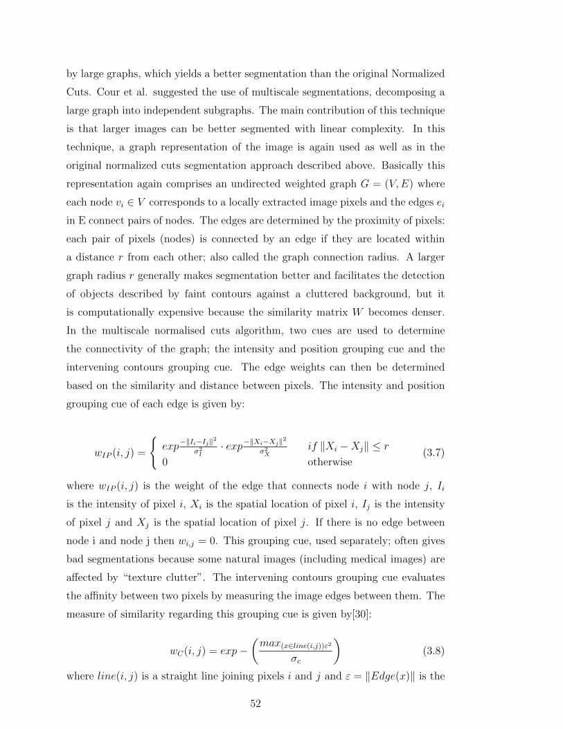
by large graphs, which yields a better segmentation than the original Normalized
Cuts. Cour et al. suggested the use of multiscale segmentations, decomposing a
large graph into independent subgraphs. The main contribution of this technique
is that larger images can be better segmented with linear complexity. In this
technique, a graph representation of the image is again used as well as in the
original normalized cuts segmentation approach described above. Basically this
representation again comprises an undirected weighted graph G = (V,E) where
each node vi ∈ V corresponds to a locally extracted image pixels and the edges ei
in E connect pairs of nodes. The edges are determined by the proximity of pixels:
each pair of pixels (nodes) is connected by an edge if they are located within
a distance r from each other; also called the graph connection radius. A larger
graph radius r generally makes segmentation better and facilitates the detection
of objects described by faint contours against a cluttered background, but it
is computationally expensive because the similarity matrix W becomes denser.
In the multiscale normalised cuts algorithm, two cues are used to determine
the connectivity of the graph; the intensity and position grouping cue and the
intervening contours grouping cue. The edge weights can then be determined
based on the similarity and distance between pixels. The intensity and position
grouping cue of each edge is given by:
wIP (i, j) =
{exp
−‖Ii−Ij‖2
σ2I· exp−‖Xi−Xj‖
2
σ2X
if ‖Xi −Xj‖ ≤ r
0 otherwise(3.7)
where wIP (i, j) is the weight of the edge that connects node i with node j, Ii
is the intensity of pixel i, Xi is the spatial location of pixel i, Ij is the intensity
of pixel j and Xj is the spatial location of pixel j. If there is no edge between
node i and node j then wi,j = 0. This grouping cue, used separately; often gives
bad segmentations because some natural images (including medical images) are
affected by “texture clutter”. The intervening contours grouping cue evaluates
the affinity between two pixels by measuring the image edges between them. The
measure of similarity regarding this grouping cue is given by[30]:
wC(i, j) = exp−(max(x∈line(i,j))ε2
σc
)(3.8)
where line(i, j) is a straight line joining pixels i and j and ε = ‖Edge(x)‖ is the
52
image strength at location x. These two cues can be combined as shown by[30]:
w(i, j) =√wIP (i, j) wC(i, j) + wC(i, j) (3.9)
The multiscale normalized cut algorithm [30] works on multiple scales of the
image so as to capture both coarse and fine levels of details. The construction of
the image segmentation graph is given according to their spatial separation, as
in:
W = W1 +W2 + ...+Ws, (3.10)
where W represents the graph weights w(i, j) and s the scale, i.e. Ws contains
similarity measure between pixels with certain scale s. Two pixels i, j are con-
nected only if rs−1 < ‖Xi −Xj‖ ≤ rs. The r value is a tradeoff between the
computation cost and the segmentation result. The decomposition graph above
can alleviate this situation. Ws can be compressed using recursive sub-sampling
of the image pixels. Cour et al. determine representative pixels at each scale s as
follows. First they sample representative pixels at (2r + 1)s−1 distance apart on
the original image grid, and denote the representative pixels at each scale s by
Is and denote W cs as a compressed similarity matrix with connections between
representative pixels in Is, i.e. for the first graph scale, every pixel is a graph
node and two nodes are connected with a graph edge if the two pixels are within
r distance apart. They then construct W c1 as a compressed similarity matrix with
connections between representative pixels in I1. For the second graph scale, they
consider pixels at distance 2r+1 apart in the original grid as representative nodes,
I2 and construct W c2 as a compressed similarity matrix with connections between
representative pixels in I2. For the third graph scale, they consider pixels at dis-
tance (2r+1)2 apart in the original grid as representative nodes, I3 and construct
W c3 as a compressed similarity matrix with connections between representative
pixels in I3. In general, they consider pixels at distance (2r + 1)(s−1) apart in
the original grid as representative nodes, Is. Then the full multiscale similirity
matrix W can be expressed as:
W =
W c1 0
. . .
0 W cs
(3.11)
53
Cour et al. reformulated the constrained multiscale normalized cut into the
following formula:
maximize ϕ(X) =1
K
K∑l=1
XTl WXl
XTl DXl
subject to : CX = 0 (3.12)
where X is an indicator vector s.t. X ∈ {0, 1}N∗×K , N∗ =∑
sNs, Ns is the
number of representative pixels in Is. The cross-scale constraint matrix C:
C =
C1,2 −I2 0. . . . . .
0 CS−1,S −IS
(3.13)
where Cs,s+1(i, j) = 1|Ni| if j ∈ Ni and Ni is the neighbourhood which specifies
the projection of i ∈ Is+1 on the finer layer Is.
The NP-complete constrained normalized cut is thus transformed into the
following eigenvalue problem:
W X = λX (3.14)
where:
W = QD−1/2WD−1/2Q (3.15)
and
Q = I −D−1/2CT (CD−1CT )−1CD−1/2 (3.16)
The K first eigenvectors of W is used to find the indicator vectors X to segment
the image into K partitions.
From the above, the image segmentation procedure based on multiscale nor-
malized cuts can be summarized as follows:
1. Given an m× n image I, for s = 1..S (S = number of scales):
(a) Sample mρ× n
ρpixels i ∈ Is from Is−1, where ρ is the sampling factor.
(b) Compute constraint Cs,s+1(i, j) = 1|Ni| , j ∈ Ni sampling neighbour-
hood of i.
54
(c) Compute the similarity matrix W cs for the representative pixels Is.
2. Compute W , C from (Ws, Cs−1,s) as in (3.11),(3.13).
3. Solve the eigensystem W X = λX as in (3.15), (3.16).
4. Use the first k eigenvectors of W to partition the image into k segments.
The multiscale normalized cuts algorithm has been shown to work well in
many studies; however it was found that, in the context of the corpus callosum
application, the algorithm did not work as well as expected with respect to all
brain MRI scans in the test data sets. This was because: (i) MRI brain scans
include a lot of noises, (ii) the intensity-level distributions between different soft
tissues were not widely distributed and (iii) the complexity of tissue boundaries
caused many pixels to contain mixtures of tissues. Although one can visually
recognize the outline of the corpus callosum (Figure 3.1), portions of its bound-
ary are indistinct, which can make it difficult to apply segmentation algorithms
based on edge information alone. A further problem is that, quite often, intensity
variations within the corpus callosum can be comparable or exceed the difference
with the surrounding tissues. For these reasons it is desirable to enhance the con-
trast of the MR images. A variation of the multiscale normalized cuts algorithm
was therefore developed. This is described in the following Subsection 3.4.4.
3.4.4 Proposed Approach
As noted above, the multiscale normalized cuts algorithm when applied to brain
MRI scans to delineate the corpus callosum within these scans did not give satis-
factory results with respect to all brain MRI scans in the test data. In the case of
some scans the corpus callosum region can be clearly identified as shown in Figure
3.3 but blurred into other surrounding tissues in some other scans. Therefore a
variation of the multiscale normalized cuts algorithm was developed that applied
a threshold interval to extract objects with the same intensity values (such as the
corpus callosum) during the application of the segmentation. This was found to
give a much improved result.
The proposed variation of the multiscale normalized cuts algorithm was founded
on the observation that the corpus callosum, which is located at the centre of the
55
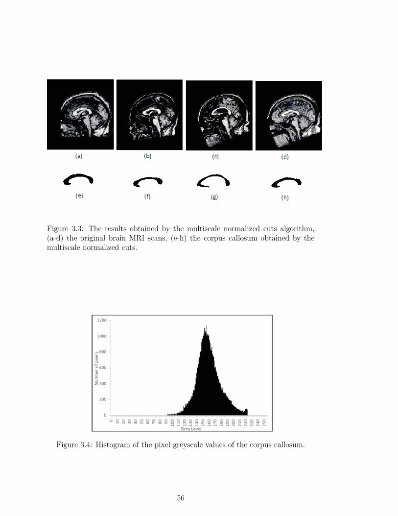
Figure 3.3: The results obtained by the multiscale normalized cuts algorithm,(a-d) the original brain MRI scans, (e-h) the corpus callosum obtained by themultiscale normalized cuts.
Figure 3.4: Histogram of the pixel greyscale values of the corpus callosum.
56
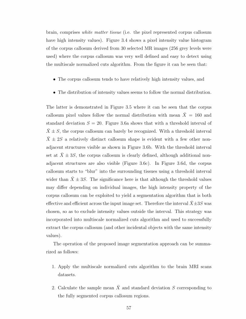
brain, comprises white matter tissue (i.e. the pixel represented corpus callosum
have high intensity values). Figure 3.4 shows a pixel intensity value histogram
of the corpus callosum derived from 30 selected MR images (256 grey levels were
used) where the corpus callosum was very well defined and easy to detect using
the multiscale normalized cuts algorithm. From the figure it can be seen that:
• The corpus callosum tends to have relatively high intensity values, and
• The distribution of intensity values seems to follow the normal distribution.
The latter is demonstrated in Figure 3.5 where it can be seen that the corpus
callosum pixel values follow the normal distribution with mean X = 160 and
standard deviation S = 20. Figure 3.6a shows that with a threshold interval of
X ± S, the corpus callosum can barely be recognized. With a threshold interval
X ± 2S a relatively distinct callosum shape is evident with a few other non-
adjacent structures visible as shown in Figure 3.6b. With the threshold interval
set at X ± 3S, the corpus callosum is clearly defined, although additional non-
adjacent structures are also visible (Figure 3.6c). In Figure 3.6d, the corpus
callosum starts to “blur” into the surrounding tissues using a threshold interval
wider than X ± 3S. The significance here is that although the threshold values
may differ depending on individual images, the high intensity property of the
corpus callosum can be exploited to yield a segmentation algorithm that is both
effective and efficient across the input image set. Therefore the interval X±3S was
chosen, so as to exclude intensity values outside the interval. This strategy was
incorporated into multiscale normalized cuts algorithm and used to successfully
extract the corpus callosum (and other incidental objects with the same intensity
values).
The operation of the proposed image segmentation approach can be summa-
rized as follows:
1. Apply the multiscale normalized cuts algorithm to the brain MRI scans
datasets.
2. Calculate the sample mean X and standard deviation S corresponding to
the fully segmented corpus callosum regions.
57
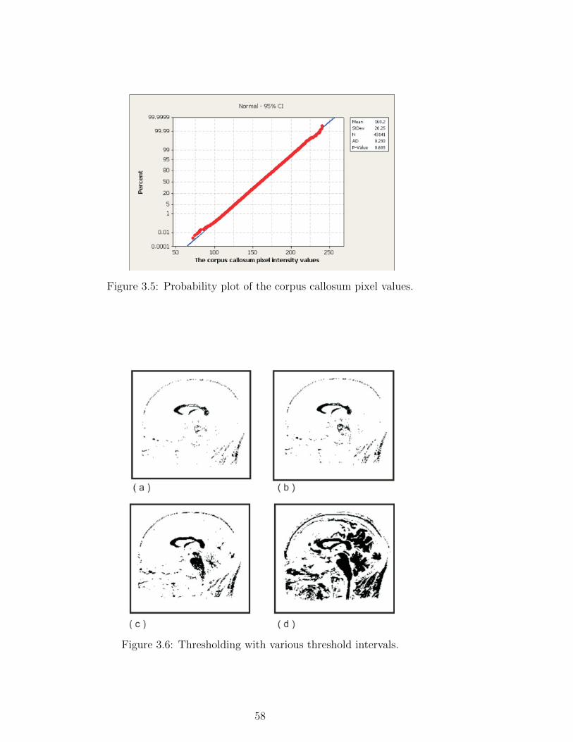
Figure 3.5: Probability plot of the corpus callosum pixel values.
Figure 3.6: Thresholding with various threshold intervals.
58
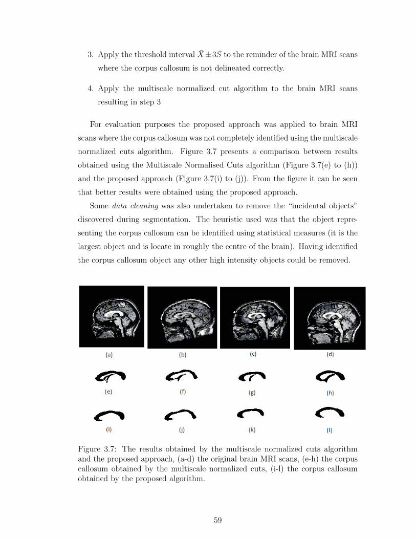
3. Apply the threshold interval X±3S to the reminder of the brain MRI scans
where the corpus callosum is not delineated correctly.
4. Apply the multiscale normalized cut algorithm to the brain MRI scans
resulting in step 3
For evaluation purposes the proposed approach was applied to brain MRI
scans where the corpus callosum was not completely identified using the multiscale
normalized cuts algorithm. Figure 3.7 presents a comparison between results
obtained using the Multiscale Normalised Cuts algorithm (Figure 3.7(e) to (h))
and the proposed approach (Figure 3.7(i) to (j)). From the figure it can be seen
that better results were obtained using the proposed approach.
Some data cleaning was also undertaken to remove the “incidental objects”
discovered during segmentation. The heuristic used was that the object repre-
senting the corpus callosum can be identified using statistical measures (it is the
largest object and is locate in roughly the centre of the brain). Having identified
the corpus callosum object any other high intensity objects could be removed.
Figure 3.7: The results obtained by the multiscale normalized cuts algorithmand the proposed approach, (a-d) the original brain MRI scans, (e-h) the corpuscallosum obtained by the multiscale normalized cuts, (i-l) the corpus callosumobtained by the proposed algorithm.
59
3.5 Medical Image Datasets
To evaluate the ROIBIC techniques described in this thesis to classify medical
images according to a particular object that features across the data sets a num-
ber of data sets were used. As already noted the data sets were generated by
extracting the midsagittal slice from MRI brain scan data volumes (bundles), one
image per volume. Each data set thus comprised a number of brain MRI scans
each measuring 256× 256 pixels, with 256 greyscale levels and each describing a
midsagittal slice. To support the evaluation the data sets were grouped as fol-
lows: (i) musicians, (ii) handedness and (iii) epilepsy. Each group is described in
some further detail as follows:
Musicians datasets. For the musicians study the data set comprising 106 MRI
scans, 53 representing musicians and 53 non-musicians (i.e. two equal
classes). The study was of interest because of the conjecture that the size
and shape of the corpus callosum reflects human characteristics (such as a
musical or mathematical ability) [111, 132].
Handedness datasets. For the handedness study a data set comprising 82 MRI
scans was used, 42 representing right handed individuals and 40 left handed
individuals. The study was of interest because of the conjecture that the
size and shape of the corpus callosum reflects certain human characteristics
(such as handedness) [31].
Epilepsy datasets. For the epilepsy study three data sets (Ep106, Ep159 and
Ep212)were used. The first data set, Ep106,comprised the control group from
the musicians study (the non-musicians) and 53 MRI scans from epilepsy
patients so as to give a balanced data set. The second data set, Ep159, used
all 106 MRI scans from the musicians study and 53 epilepsy scans. The
third data set, Ep212 was the same as the second but augmented with a
further 53 epilepsy cases to create a balanced data set. The objective was
to seek support for the conjecture that the shape and size of the corpus
callosum is influence by conditions such as epilepsy [27, 124, 149].
All three brain MRI datasets were preprocessed using the variation of the mul-
tiscale normalized cuts algorithm described above (Subsection 3.4.4) to extract
60
the corpus callosum feature. On completion of data cleaning a “local” registration
process was undertaken by fitting each identified corpus callosum into a Minimum
Bounding Rectangle (MBR) so that each identified corpus callosum was founded
upon the same origin.
3.6 Summary
This chapter has provided the necessary context to the preprocessing of the brain
MRI scan data so as to detect and extract the desired ROI (the corpus callosum).
A variation of the multiscale normalized cuts algorithm was proposed to achieve
the desired segmentation. A description of the medical image datasets, used
for evaluation purposes later in this thesis, was also given. In the following
four chapters the four different techniques, whereby MRI brain scan data can be
classified according to a particular ROI (namely the corpus callosum), considered
in this thesis are described and evaluated. The first technique considered is the
Hough Transform technique which is presented in the following chapter.
61

62
Chapter 4
Region Of Interest ImageClassification Using a HoughTransform SignatureRepresentation
4.1 Introduction
As noted in Chapter 2 the Hough transform was first introduced by Paul Hough
in 1962 [67]. It later became the basis for a great number of image analysis
techniques with respect to many applications. The Hough transform is mainly
used to detect parametric shapes in images. It was first used to detect straight
lines and later extended to other parametric models such as circles or ellipses,
being finally generalized to detect any parametric shape [12]. The key idea of
the Hough transform is that spatially extended patterns are transformed into
a parameter space where they can be represented in a spatially compact way.
Thus, a difficult global detection problem in the image space is reduced to an
easier problem of peak detection in a parameter space. A set of collinear image
points (x, y) can be represented by the equation:
y −mx− c = 0 (4.1)
where m and c are the standard parameters slope and intercept, which character-
ize the line equations. Equation 4.1 maps each value of the parameter combination
(m, c) to a set of image points. But Equation 4.1 can be “read” as a backpro-
jection, i.e. it represents the set of straight lines, each defined by a point (m, c)
63
in the parameter space, passing through an image point (x, y). From this point
of view, each image point (x, y) defines a straight line in the parameter space
which represents all possible combinations of (m, c) that defining a line passing
through (x, y). Points which are collinear in the image space all intersect at a
common point in the parameter space and the coordinates of this point charac-
terizes the straight line connecting the image points. Thus, the problem of line
detection in the image space is transformed to the problem of finding intersection
points (peaks) in the parameter space, a much simpler problem to resolve. The
straight line Hough transform can easily be extended to detect other parametri-
cally defined curves that may be contained in an image. Image points of a curve
characterized by n parameters α1, ..., αn can be defined by an equation of the
form:
f(α1, ..., αn, x, y) = 0 (4.2)
Following the same idea, an image point (x, y) can be used to define a hy-
persurface in some n-dimensional parameter space (α1, ..., αn) . The intersections
of such hypersurfaces indicate the parameters which are likely to characterize
instances of the searched curves in the image space. The Hough transform offers
several advantages:
1. Each image point is treated independently and therefore parallel processing
is possible, consequently the method is suitable for real-time applications,
such as CCTV surveillance analysis.
2. The method is robust to the presence of noise since noisy image points are
very unlikely to contribute to a peak in the parameter space.
3. Since each image point contributes independently to the set of parameter
space points, the algorithm is able to work even if the shape is occluded.
4. The Hough transform is able to detect different instances of the desired
shape at the same time, depending on the number of peaks which are con-
sidered in the parameter space.
The main drawbacks of the Hough transform are its large storage and compu-
tational requirements. The computational load can be reduced by using informa-
64
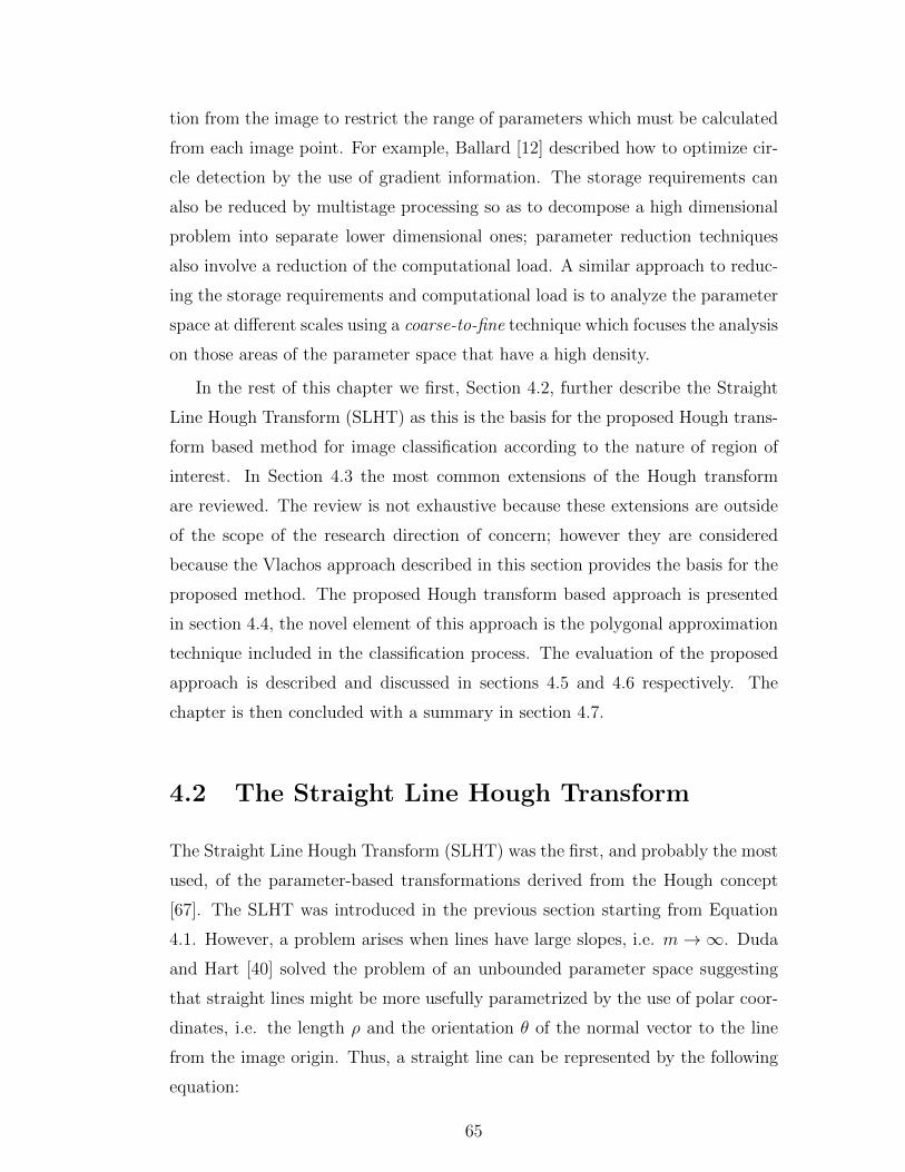
tion from the image to restrict the range of parameters which must be calculated
from each image point. For example, Ballard [12] described how to optimize cir-
cle detection by the use of gradient information. The storage requirements can
also be reduced by multistage processing so as to decompose a high dimensional
problem into separate lower dimensional ones; parameter reduction techniques
also involve a reduction of the computational load. A similar approach to reduc-
ing the storage requirements and computational load is to analyze the parameter
space at different scales using a coarse-to-fine technique which focuses the analysis
on those areas of the parameter space that have a high density.
In the rest of this chapter we first, Section 4.2, further describe the Straight
Line Hough Transform (SLHT) as this is the basis for the proposed Hough trans-
form based method for image classification according to the nature of region of
interest. In Section 4.3 the most common extensions of the Hough transform
are reviewed. The review is not exhaustive because these extensions are outside
of the scope of the research direction of concern; however they are considered
because the Vlachos approach described in this section provides the basis for the
proposed method. The proposed Hough transform based approach is presented
in section 4.4, the novel element of this approach is the polygonal approximation
technique included in the classification process. The evaluation of the proposed
approach is described and discussed in sections 4.5 and 4.6 respectively. The
chapter is then concluded with a summary in section 4.7.
4.2 The Straight Line Hough Transform
The Straight Line Hough Transform (SLHT) was the first, and probably the most
used, of the parameter-based transformations derived from the Hough concept
[67]. The SLHT was introduced in the previous section starting from Equation
4.1. However, a problem arises when lines have large slopes, i.e. m→∞. Duda
and Hart [40] solved the problem of an unbounded parameter space suggesting
that straight lines might be more usefully parametrized by the use of polar coor-
dinates, i.e. the length ρ and the orientation θ of the normal vector to the line
from the image origin. Thus, a straight line can be represented by the following
equation:
65
ρ = xcosθ + ysinθ (4.3)
In the conventional implementation, the Hough transform essentially consists
of three stages:
1. Characteristic point detection. Not all the image points (pixels) are
mapped to the parameter space. An information reduction process is first
applied to the image in such a way that it preserves the shapes to be de-
tected. To achieve this some image pixels are selected according to certain
local properties (e.g. gradient magnitude and gradient orientation). Usually
the information reduction process comprises local edge detection.
2. Transform mapping. Each characteristic point of the image space is
mapped to the parameter space. This parameter space is represented by a
two-dimensional accumulator array (n-dimensional for detection of higher-
order shapes). A voting rule usually underlies the transform mapping. This
voting rule determines how the transform mapping affects the contents of
the accumulator array. The simplest voting rule is to increment the polar
parameter points (ρ, θ) mapped from an image point (x, y).
3. Peak detection. The final stage is to extract the corresponding parame-
ter values of the detected shape from the accumulator array. The simplest
method is to apply some form of global thresholding on the accumulator
array. The threshold is chosen either using prior knowledge, or it can be
automatically selected by analysing the distribution of counts in the accu-
mulator array, e.g. a fixed fraction of the maximum count on any single
accumulator bin. Since the presence of noise and distortion may result in
true peaks being split between several accumulator cells and, thus causing
them not to be detected, different kinds of clustering procedures are also
applied.
Two types of Hough transform are usually distinguished depending on the
representation which is used:
• One to many (1-m). Each characteristic point (x, y) of the image space is
mapped to m points in the parameter space which represent the m possible
66
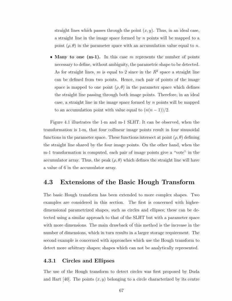
straight lines which passes through the point (x, y). Thus, in an ideal case,
a straight line in the image space formed by n points will be mapped to a
point (ρ, θ) in the parameter space with an accumulation value equal to n.
• Many to one (m-1). In this case m represents the number of points
necessary to define, without ambiguity, the parametric shape to be detected.
As for straight lines, m is equal to 2 since in the R2 space a straight line
can be defined from two points. Hence, each pair of points of the image
space is mapped to one point (ρ, θ) in the parameter space which defines
the straight line passing through both image points. Therefore, in an ideal
case, a straight line in the image space formed by n points will be mapped
to an accumulation point with value equal to (n(n− 1))/2.
Figure 4.1 illustrates the 1-m and m-1 SLHT. It can be observed, when the
transformation is 1-m, that four collinear image points result in four sinusoidal
functions in the parameter space. These functions intersect at point (ρ, θ) defining
the straight line shared by the four image points. On the other hand, when the
m-1 transformation is computed, each pair of image points give a “vote” in the
accumulator array. Thus, the peak (ρ, θ) which defines the straight line will have
a value of 6 in the accumulator array.
4.3 Extensions of the Basic Hough Transform
The basic Hough transform has been extended to more complex shapes. Two
examples are considered in this section. The first is concerned with higher-
dimensional parametrized shapes, such as circles and ellipses; these can be de-
tected using a similar approach to that of the SLHT but with a parameter space
with more dimensions. The main drawback of this method is the increase in the
number of dimensions, which in turn results in a larger storage requirement. The
second example is concerned with approaches which use the Hough transform to
detect more arbitrary shapes; shapes which can not be analytically represented.
4.3.1 Circles and Ellipses
The use of the Hough transform to detect circles was first proposed by Duda
and Hart [40]. The points (x, y) belonging to a circle characterized by its centre
67
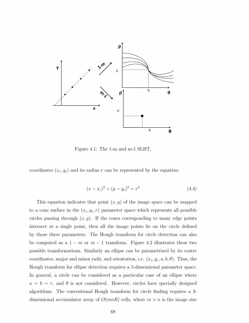
ρi
θ
y
ρρρρ
θi
x
θθθθ
ρi
θi θθθθ
ρρρρ
Figure 4.1: The 1-m and m-1 SLHT.
coordinates (xc, yc) and its radius r can be represented by the equation:
(x− xc)2 + (y − yc)2 = r2 (4.4)
This equation indicates that point (x, y) of the image space can be mapped
to a cone surface in the (xc, yc, r) parameter space which represents all possible
circles passing through (x, y). If the cones corresponding to many edge points
intersect at a single point, then all the image points lie on the circle defined
by those three parameters. The Hough transform for circle detection can also
be computed as a 1 − m or m − 1 transform. Figure 4.2 illustrates these two
possible transformations. Similarly an ellipse can be parametrized by its centre
coordinates, major and minor radii, and orientation, i.e. (xc, yc, a, b, θ). Thus, the
Hough transform for ellipse detection requires a 5-dimensional parameter space.
In general, a circle can be considered as a particular case of an ellipse where
a = b = r, and θ is not considered. However, circles have specially designed
algorithms. The conventional Hough transform for circle finding requires a 3-
dimensional accumulator array of O(mnR) cells, where m × n is the image size
68
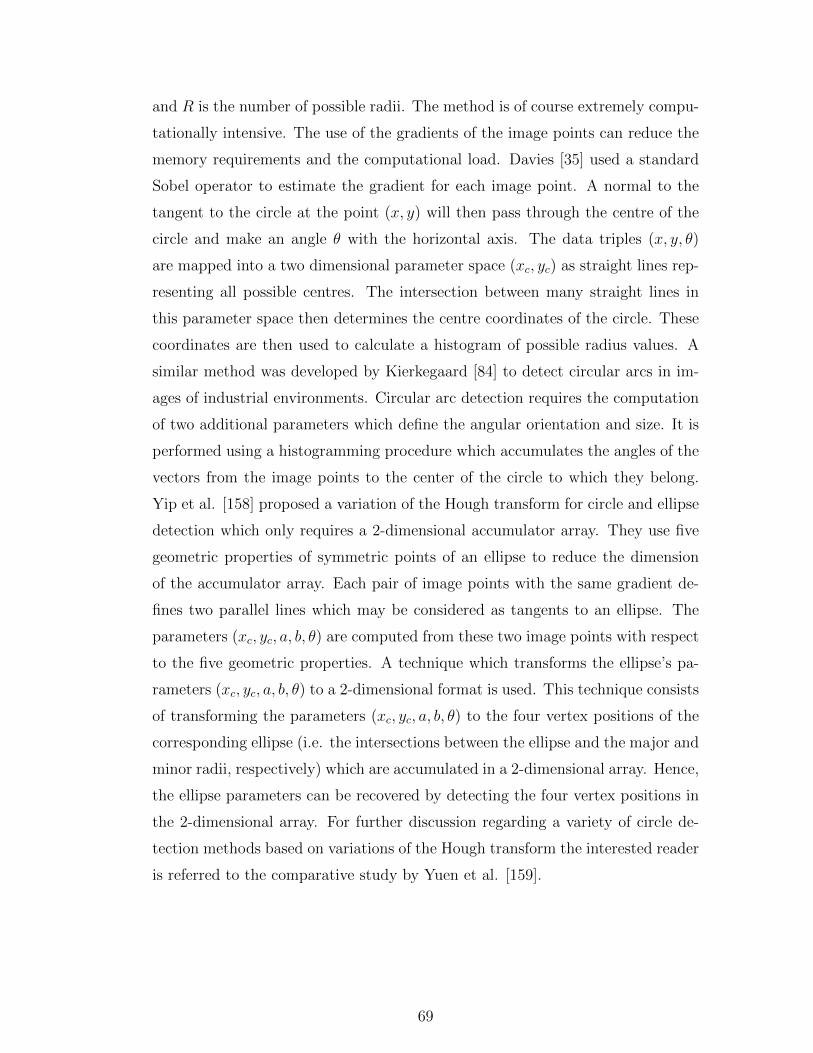
and R is the number of possible radii. The method is of course extremely compu-
tationally intensive. The use of the gradients of the image points can reduce the
memory requirements and the computational load. Davies [35] used a standard
Sobel operator to estimate the gradient for each image point. A normal to the
tangent to the circle at the point (x, y) will then pass through the centre of the
circle and make an angle θ with the horizontal axis. The data triples (x, y, θ)
are mapped into a two dimensional parameter space (xc, yc) as straight lines rep-
resenting all possible centres. The intersection between many straight lines in
this parameter space then determines the centre coordinates of the circle. These
coordinates are then used to calculate a histogram of possible radius values. A
similar method was developed by Kierkegaard [84] to detect circular arcs in im-
ages of industrial environments. Circular arc detection requires the computation
of two additional parameters which define the angular orientation and size. It is
performed using a histogramming procedure which accumulates the angles of the
vectors from the image points to the center of the circle to which they belong.
Yip et al. [158] proposed a variation of the Hough transform for circle and ellipse
detection which only requires a 2-dimensional accumulator array. They use five
geometric properties of symmetric points of an ellipse to reduce the dimension
of the accumulator array. Each pair of image points with the same gradient de-
fines two parallel lines which may be considered as tangents to an ellipse. The
parameters (xc, yc, a, b, θ) are computed from these two image points with respect
to the five geometric properties. A technique which transforms the ellipse’s pa-
rameters (xc, yc, a, b, θ) to a 2-dimensional format is used. This technique consists
of transforming the parameters (xc, yc, a, b, θ) to the four vertex positions of the
corresponding ellipse (i.e. the intersections between the ellipse and the major and
minor radii, respectively) which are accumulated in a 2-dimensional array. Hence,
the ellipse parameters can be recovered by detecting the four vertex positions in
the 2-dimensional array. For further discussion regarding a variety of circle de-
tection methods based on variations of the Hough transform the interested reader
is referred to the comparative study by Yuen et al. [159].
69
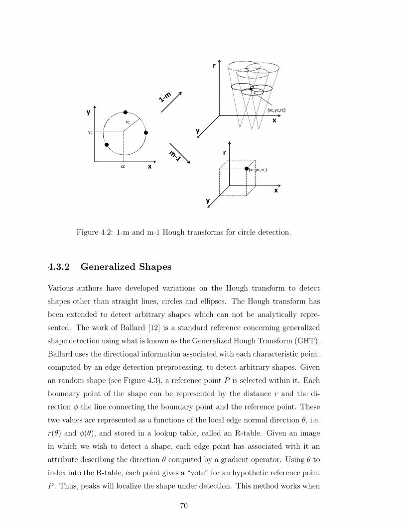
y
x
y
r
(xc,yc,rc)
yc
rc
x
y
x
y
r
xc
yc
(xc,yc,rc)
Figure 4.2: 1-m and m-1 Hough transforms for circle detection.
4.3.2 Generalized Shapes
Various authors have developed variations on the Hough transform to detect
shapes other than straight lines, circles and ellipses. The Hough transform has
been extended to detect arbitrary shapes which can not be analytically repre-
sented. The work of Ballard [12] is a standard reference concerning generalized
shape detection using what is known as the Generalized Hough Transform (GHT).
Ballard uses the directional information associated with each characteristic point,
computed by an edge detection preprocessing, to detect arbitrary shapes. Given
an random shape (see Figure 4.3), a reference point P is selected within it. Each
boundary point of the shape can be represented by the distance r and the di-
rection φ the line connecting the boundary point and the reference point. These
two values are represented as a functions of the local edge normal direction θ, i.e.
r(θ) and φ(θ), and stored in a lookup table, called an R-table. Given an image
in which we wish to detect a shape, each edge point has associated with it an
attribute describing the direction θ computed by a gradient operator. Using θ to
index into the R-table, each point gives a “vote” for an hypothetic reference point
P . Thus, peaks will localize the shape under detection. This method works when
70
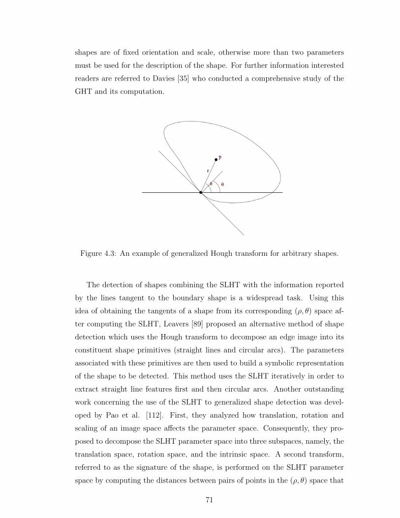
shapes are of fixed orientation and scale, otherwise more than two parameters
must be used for the description of the shape. For further information interested
readers are referred to Davies [35] who conducted a comprehensive study of the
GHT and its computation.
Figure 4.3: An example of generalized Hough transform for arbitrary shapes.
The detection of shapes combining the SLHT with the information reported
by the lines tangent to the boundary shape is a widespread task. Using this
idea of obtaining the tangents of a shape from its corresponding (ρ, θ) space af-
ter computing the SLHT, Leavers [89] proposed an alternative method of shape
detection which uses the Hough transform to decompose an edge image into its
constituent shape primitives (straight lines and circular arcs). The parameters
associated with these primitives are then used to build a symbolic representation
of the shape to be detected. This method uses the SLHT iteratively in order to
extract straight line features first and then circular arcs. Another outstanding
work concerning the use of the SLHT to generalized shape detection was devel-
oped by Pao et al. [112]. First, they analyzed how translation, rotation and
scaling of an image space affects the parameter space. Consequently, they pro-
posed to decompose the SLHT parameter space into three subspaces, namely, the
translation space, rotation space, and the intrinsic space. A second transform,
referred to as the signature of the shape, is performed on the SLHT parameter
space by computing the distances between pairs of points in the (ρ, θ) space that
71
have the same θ value. This is equivalent to computing the perpendicular dis-
tances between pairs of parallel tangents to the curves. This signature has the
following properties: (i) it is invariant to translation, (ii) rotations in the image
space correspond to circular shiftings of the signature, and (iii) it can be easily
normalized. The recognition of a shape is performed by a one-dimensional corre-
lation between the candidate signature and the normalized model signature. The
peak of this correlation also indicates the orientation of the object. Finally, the
location of the shape is obtained by an inverse transform from the (ρ, θ) space to
the (x, y) space. In [145], Vlachos et al. adopted the SLHT to extract a region
signature to be used in the image classification process. They use the projection
of the accumulator array from ρ− θ space to θ space. Then the region signature
can be expressed as one dimensional vector in terms of θ after the normalization
of that vector by dividing it by its mean value. The significance of Vlachos ap-
proach with respect to this thesis is that it has been adopted for the proposed
Hough transform based ROIBIC process.
4.4 Proposed Image Classification Method
The proposed image classification based on the Hough transform focuses primarily
on the extracting of shape signatures which can be used as a feature vector in the
classification process. Therefore, it is assumed that the input image is a binary
representation of a region of interest (i.e. the corpus callosum with respect to the
focus of the work described in this thesis), that has been appropriately segmented
from “source” MRI brain scans of the form previously described in Chapter 3. The
proposed shape signature extraction method is founded on that first presented in
Vlachos et al. [145] which was briefly described in Subsection 4.3.2. This method
gives good results when classifying simple line drawn symbol images according to
their shapes. However, Vlachos approach was found to perform consistently badly
with respect to the classification of brain MRI scans according to the nature of
the corpus callosum. Therefore the proposed method commences by simplifying
the shape of the region of interest within the MRI brain scans using a polygonal
approximation method. Then the signature extraction process, using Vlachos
approach, was applied.
The proposed image classification technique based on the Hough transform is
72
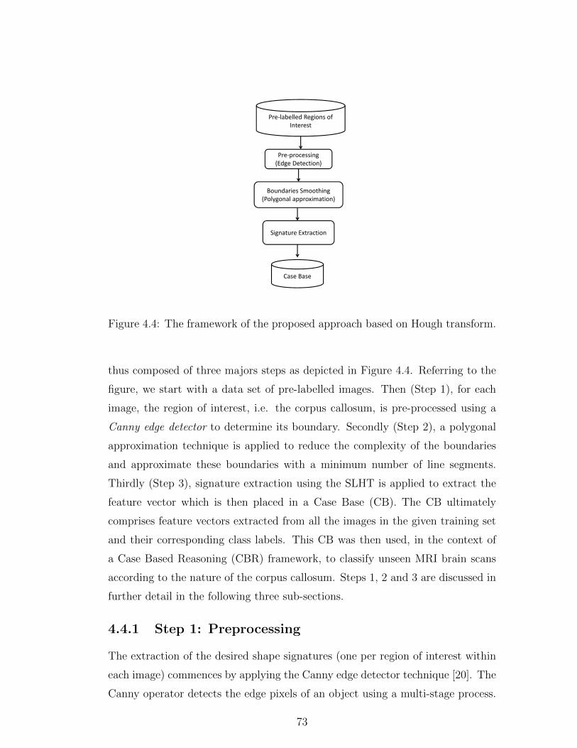
Pre-labelled Regions of
Interest
Pre-processing
(Edge Detection)
Boundaries Smoothing
(Polygonal approximation)
Signature Extraction
Case Base
Figure 4.4: The framework of the proposed approach based on Hough transform.
thus composed of three majors steps as depicted in Figure 4.4. Referring to the
figure, we start with a data set of pre-labelled images. Then (Step 1), for each
image, the region of interest, i.e. the corpus callosum, is pre-processed using a
Canny edge detector to determine its boundary. Secondly (Step 2), a polygonal
approximation technique is applied to reduce the complexity of the boundaries
and approximate these boundaries with a minimum number of line segments.
Thirdly (Step 3), signature extraction using the SLHT is applied to extract the
feature vector which is then placed in a Case Base (CB). The CB ultimately
comprises feature vectors extracted from all the images in the given training set
and their corresponding class labels. This CB was then used, in the context of
a Case Based Reasoning (CBR) framework, to classify unseen MRI brain scans
according to the nature of the corpus callosum. Steps 1, 2 and 3 are discussed in
further detail in the following three sub-sections.
4.4.1 Step 1: Preprocessing
The extraction of the desired shape signatures (one per region of interest within
each image) commences by applying the Canny edge detector technique [20]. The
Canny operator detects the edge pixels of an object using a multi-stage process.
73
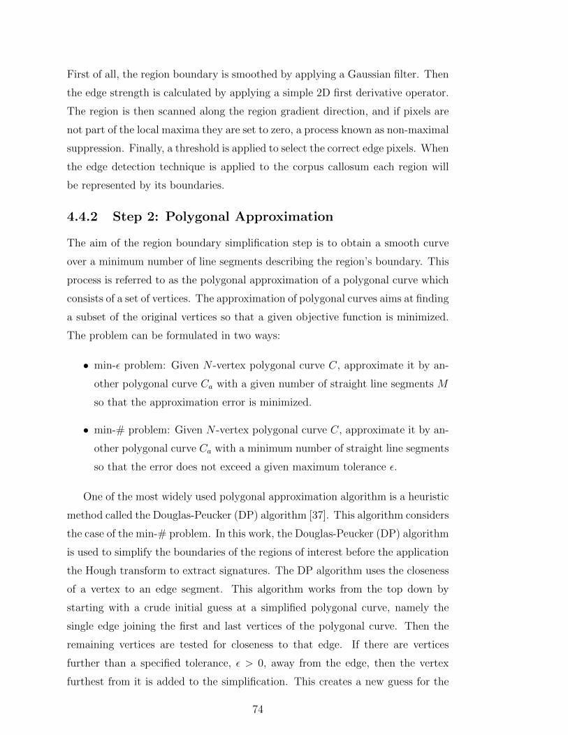
First of all, the region boundary is smoothed by applying a Gaussian filter. Then
the edge strength is calculated by applying a simple 2D first derivative operator.
The region is then scanned along the region gradient direction, and if pixels are
not part of the local maxima they are set to zero, a process known as non-maximal
suppression. Finally, a threshold is applied to select the correct edge pixels. When
the edge detection technique is applied to the corpus callosum each region will
be represented by its boundaries.
4.4.2 Step 2: Polygonal Approximation
The aim of the region boundary simplification step is to obtain a smooth curve
over a minimum number of line segments describing the region’s boundary. This
process is referred to as the polygonal approximation of a polygonal curve which
consists of a set of vertices. The approximation of polygonal curves aims at finding
a subset of the original vertices so that a given objective function is minimized.
The problem can be formulated in two ways:
• min-ε problem: Given N -vertex polygonal curve C, approximate it by an-
other polygonal curve Ca with a given number of straight line segments M
so that the approximation error is minimized.
• min-# problem: Given N -vertex polygonal curve C, approximate it by an-
other polygonal curve Ca with a minimum number of straight line segments
so that the error does not exceed a given maximum tolerance ε.
One of the most widely used polygonal approximation algorithm is a heuristic
method called the Douglas-Peucker (DP) algorithm [37]. This algorithm considers
the case of the min-# problem. In this work, the Douglas-Peucker (DP) algorithm
is used to simplify the boundaries of the regions of interest before the application
the Hough transform to extract signatures. The DP algorithm uses the closeness
of a vertex to an edge segment. This algorithm works from the top down by
starting with a crude initial guess at a simplified polygonal curve, namely the
single edge joining the first and last vertices of the polygonal curve. Then the
remaining vertices are tested for closeness to that edge. If there are vertices
further than a specified tolerance, ε > 0, away from the edge, then the vertex
furthest from it is added to the simplification. This creates a new guess for the
74
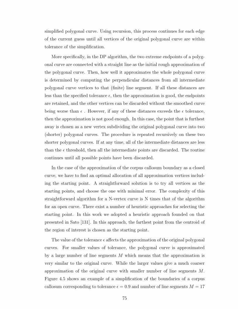
simplified polygonal curve. Using recursion, this process continues for each edge
of the current guess until all vertices of the original polygonal curve are within
tolerance of the simplification.
More specifically, in the DP algorithm, the two extreme endpoints of a polyg-
onal curve are connected with a straight line as the initial rough approximation of
the polygonal curve. Then, how well it approximates the whole polygonal curve
is determined by computing the perpendicular distances from all intermediate
polygonal curve vertices to that (finite) line segment. If all these distances are
less than the specified tolerance ε, then the approximation is good, the endpoints
are retained, and the other vertices can be discarded without the smoothed curve
being worse than ε . However, if any of these distances exceeds the ε tolerance,
then the approximation is not good enough. In this case, the point that is furthest
away is chosen as a new vertex subdividing the original polygonal curve into two
(shorter) polygonal curves. The procedure is repeated recursively on these two
shorter polygonal curves. If at any time, all of the intermediate distances are less
than the ε threshold, then all the intermediate points are discarded. The routine
continues until all possible points have been discarded.
In the case of the approximation of the corpus callosum boundary as a closed
curve, we have to find an optimal allocation of all approximation vertices includ-
ing the starting point. A straightforward solution is to try all vertices as the
starting points, and choose the one with minimal error. The complexity of this
straightforward algorithm for a N-vertex curve is N times that of the algorithm
for an open curve. There exist a number of heuristic approaches for selecting the
starting point. In this work we adopted a heuristic approach founded on that
presented in Sato [131]. In this approach, the farthest point from the centroid of
the region of interest is chosen as the starting point.
The value of the tolerance ε affects the approximation of the original polygonal
curves. For smaller values of tolerance, the polygonal curve is approximated
by a large number of line segments M which means that the approximation is
very similar to the original curve. While the larger values give a much coarser
approximation of the original curve with smaller number of line segments M .
Figure 4.5 shows an example of a simplification of the boundaries of a corpus
callosum corresponding to tolerance ε = 0.9 and number of line segments M = 17
75
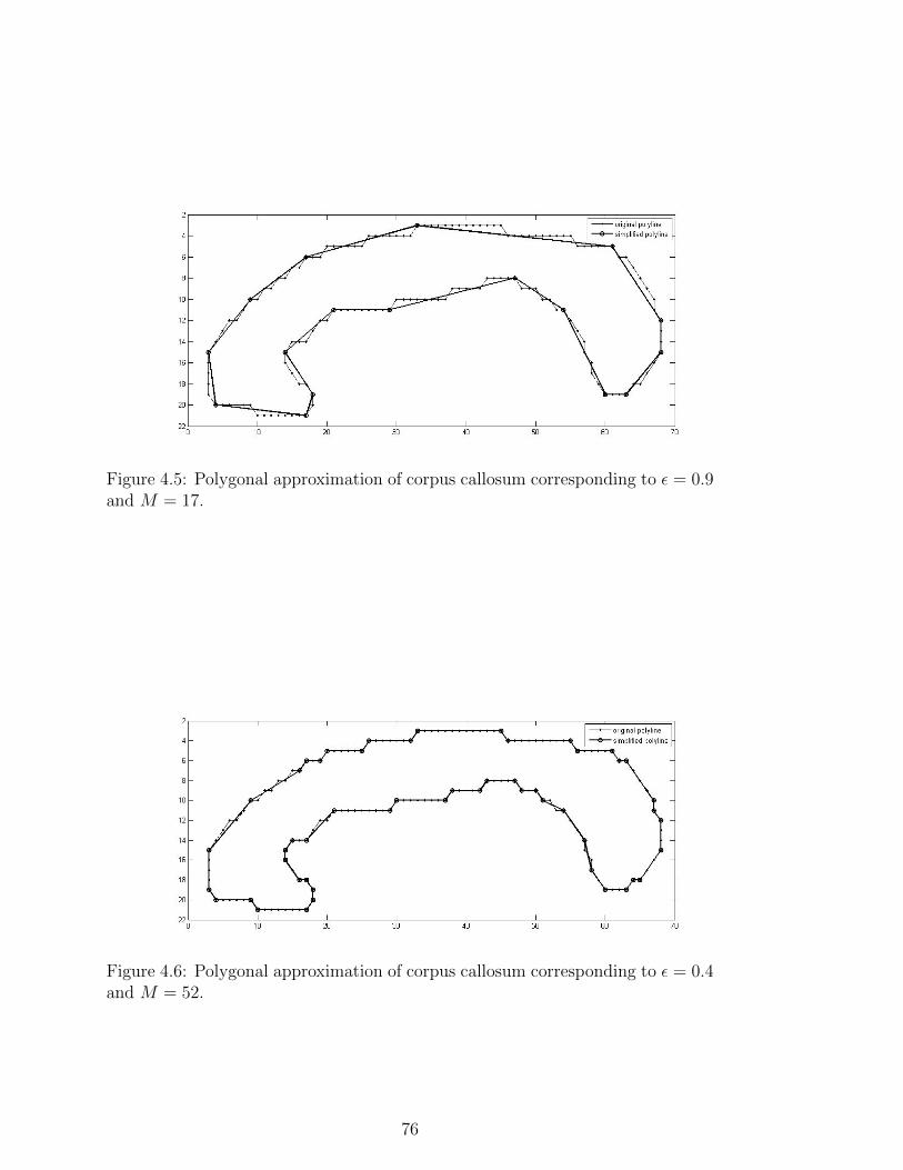
Figure 4.5: Polygonal approximation of corpus callosum corresponding to ε = 0.9and M = 17.
Figure 4.6: Polygonal approximation of corpus callosum corresponding to ε = 0.4and M = 52.
76

and Figure 4.6 shows another example of a simplification of the boundaries of the
corpus callosum corresponding to tolerance ε = 0.4 and number of line segments
M = 52.
4.4.3 Step 3: Shape Signature Extraction
The generation of the shape signature based on the Straight Line Hough Trans-
form (SLHT) relies on creating the M×N accumulator matrix A, where each row
corresponds to one value of ρ, and each column to one value of θ. The procedure
for generating the feature vector from the accumulator matrix is founded on that
presented in Vlachos et al. [145] and is as follows:
1. Determine the set of boundary pixels corresponding to the region of interest.
2. Transform each pixel in the set into a parametric curve in the parameter
space.
3. Increment the cells in the accumulator matrix A determined by the para-
metric curve.
4. Calculate a preliminary feature vector:
Fj =M∑i=1
A2ij(ρ, θ), j = 1..N
5. Calculate vector mean
µ =1
N
N∑j=1
Fj
6. Normalize the feature vector:
FVj(θ) =Fjµ, j = 1..N
In (2) the transformation can be as in Equation 4.1, where (x, y) are the
coordinates of the pixel to be transformed, and ρ and θ are the parameters of the
corresponding line. Thus, every pixel (x, y) can be seen as a curve in the (ρ, θ)
parameter space, where θ varies from the minimum to the maximum value, giving
the corresponding ρ values. By transforming every point (x, y) in the image into
the parameter space, the line parameters can be found in the intersections of the
77
parametrized curves in the accumulator matrix as show in Figure 4.1. In step 4,
the accumulator matrix is projected to a one-dimensional θ vector by summing
up the ρ values in each column. Finally the feature vector is normalized according
to its mean (5) and (6). The extracted feature vector describing the ROI within
each image can then be used as an image signature.
4.4.4 Classification
The signatures from a labelled training set can thus be collected together and
stored in a Case Base (CB) within a Case Based Reasoning (CBR) framework.
Euclidean distance may then be used as a similarity measure in the context of a
CBR framework. Let us assume that we have the feature vector T for a prelabelled
image and the feature vector Q for the test image (both of size N). Their distance
apart is calculated as:
dist(T,Q) =N∑j=1
(Tj −Qj)2
Here dist = 0 indicates identical images and dist = distmax indicates two images
with maximum dissimilarity.
To categorise “unseen” MRI brain scans, according to the nature of the corpus
callosum, signatures describing the unseen cases were compared with the signa-
tures of labelled cases held in the CB. The well established K-Nearest Neighbour
(KNN) technique was used to identify the most similar signature in the CB from
which a class label was then be extracted.
4.5 Evaluation
The evaluation of the proposed image classification approach was undertaken
in terms of classification accuracy, sensitivity and specificity. The three studies
introduced in Chapter 3 were used for the investigation: (i) a comparison between
musician and non-musician MRI scans, (ii) a comparison between left handedness
and right handedness, and (iii) an epilepsy screening process. A description of
the datasets was presented in Chapter 3.
As noted above, euclidean distance was used to calculate the similarity be-
tween the test image signature and the pre-labelled image signatures. The KNN
78
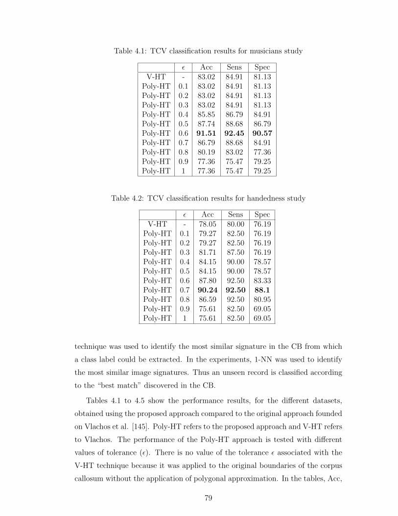
Table 4.1: TCV classification results for musicians study
ε Acc Sens SpecV-HT - 83.02 84.91 81.13
Poly-HT 0.1 83.02 84.91 81.13Poly-HT 0.2 83.02 84.91 81.13Poly-HT 0.3 83.02 84.91 81.13Poly-HT 0.4 85.85 86.79 84.91Poly-HT 0.5 87.74 88.68 86.79Poly-HT 0.6 91.51 92.45 90.57Poly-HT 0.7 86.79 88.68 84.91Poly-HT 0.8 80.19 83.02 77.36Poly-HT 0.9 77.36 75.47 79.25Poly-HT 1 77.36 75.47 79.25
Table 4.2: TCV classification results for handedness study
ε Acc Sens SpecV-HT - 78.05 80.00 76.19
Poly-HT 0.1 79.27 82.50 76.19Poly-HT 0.2 79.27 82.50 76.19Poly-HT 0.3 81.71 87.50 76.19Poly-HT 0.4 84.15 90.00 78.57Poly-HT 0.5 84.15 90.00 78.57Poly-HT 0.6 87.80 92.50 83.33Poly-HT 0.7 90.24 92.50 88.1Poly-HT 0.8 86.59 92.50 80.95Poly-HT 0.9 75.61 82.50 69.05Poly-HT 1 75.61 82.50 69.05
technique was used to identify the most similar signature in the CB from which
a class label could be extracted. In the experiments, 1-NN was used to identify
the most similar image signatures. Thus an unseen record is classified according
to the “best match” discovered in the CB.
Tables 4.1 to 4.5 show the performance results, for the different datasets,
obtained using the proposed approach compared to the original approach founded
on Vlachos et al. [145]. Poly-HT refers to the proposed approach and V-HT refers
to Vlachos. The performance of the Poly-HT approach is tested with different
values of tolerance (ε). There is no value of the tolerance ε associated with the
V-HT technique because it was applied to the original boundaries of the corpus
callosum without the application of polygonal approximation. In the tables, Acc,
79
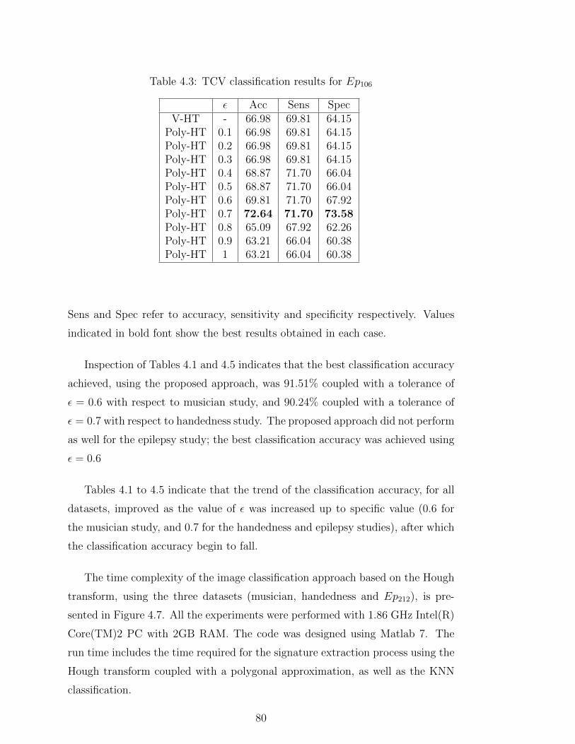
Table 4.3: TCV classification results for Ep106
ε Acc Sens SpecV-HT - 66.98 69.81 64.15
Poly-HT 0.1 66.98 69.81 64.15Poly-HT 0.2 66.98 69.81 64.15Poly-HT 0.3 66.98 69.81 64.15Poly-HT 0.4 68.87 71.70 66.04Poly-HT 0.5 68.87 71.70 66.04Poly-HT 0.6 69.81 71.70 67.92Poly-HT 0.7 72.64 71.70 73.58Poly-HT 0.8 65.09 67.92 62.26Poly-HT 0.9 63.21 66.04 60.38Poly-HT 1 63.21 66.04 60.38
Sens and Spec refer to accuracy, sensitivity and specificity respectively. Values
indicated in bold font show the best results obtained in each case.
Inspection of Tables 4.1 and 4.5 indicates that the best classification accuracy
achieved, using the proposed approach, was 91.51% coupled with a tolerance of
ε = 0.6 with respect to musician study, and 90.24% coupled with a tolerance of
ε = 0.7 with respect to handedness study. The proposed approach did not perform
as well for the epilepsy study; the best classification accuracy was achieved using
ε = 0.6
Tables 4.1 to 4.5 indicate that the trend of the classification accuracy, for all
datasets, improved as the value of ε was increased up to specific value (0.6 for
the musician study, and 0.7 for the handedness and epilepsy studies), after which
the classification accuracy begin to fall.
The time complexity of the image classification approach based on the Hough
transform, using the three datasets (musician, handedness and Ep212), is pre-
sented in Figure 4.7. All the experiments were performed with 1.86 GHz Intel(R)
Core(TM)2 PC with 2GB RAM. The code was designed using Matlab 7. The
run time includes the time required for the signature extraction process using the
Hough transform coupled with a polygonal approximation, as well as the KNN
classification.
80
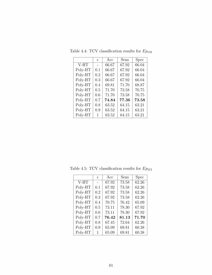
Table 4.4: TCV classification results for Ep159
ε Acc Sens SpecV-HT - 66.67 67.92 66.04
Poly-HT 0.1 66.67 67.92 66.04Poly-HT 0.2 66.67 67.92 66.04Poly-HT 0.3 66.67 67.92 66.04Poly-HT 0.4 69.81 71.70 68.87Poly-HT 0.5 71.70 73.58 70.75Poly-HT 0.6 71.70 73.58 70.75Poly-HT 0.7 74.84 77.36 73.58Poly-HT 0.8 63.52 64.15 63.21Poly-HT 0.9 63.52 64.15 63.21Poly-HT 1 63.52 64.15 63.21
Table 4.5: TCV classification results for Ep212
ε Acc Sens SpecV-HT - 67.92 73.58 62.26
Poly-HT 0.1 67.92 73.58 62.26Poly-HT 0.2 67.92 73.58 62.26Poly-HT 0.3 67.92 73.58 62.26Poly-HT 0.4 70.75 76.42 65.09Poly-HT 0.5 73.11 78.30 67.92Poly-HT 0.6 73.11 78.30 67.92Poly-HT 0.7 76.42 81.13 71.70Poly-HT 0.8 67.45 72.64 62.26Poly-HT 0.9 65.09 69.81 60.38Poly-HT 1 65.09 69.81 60.38
81
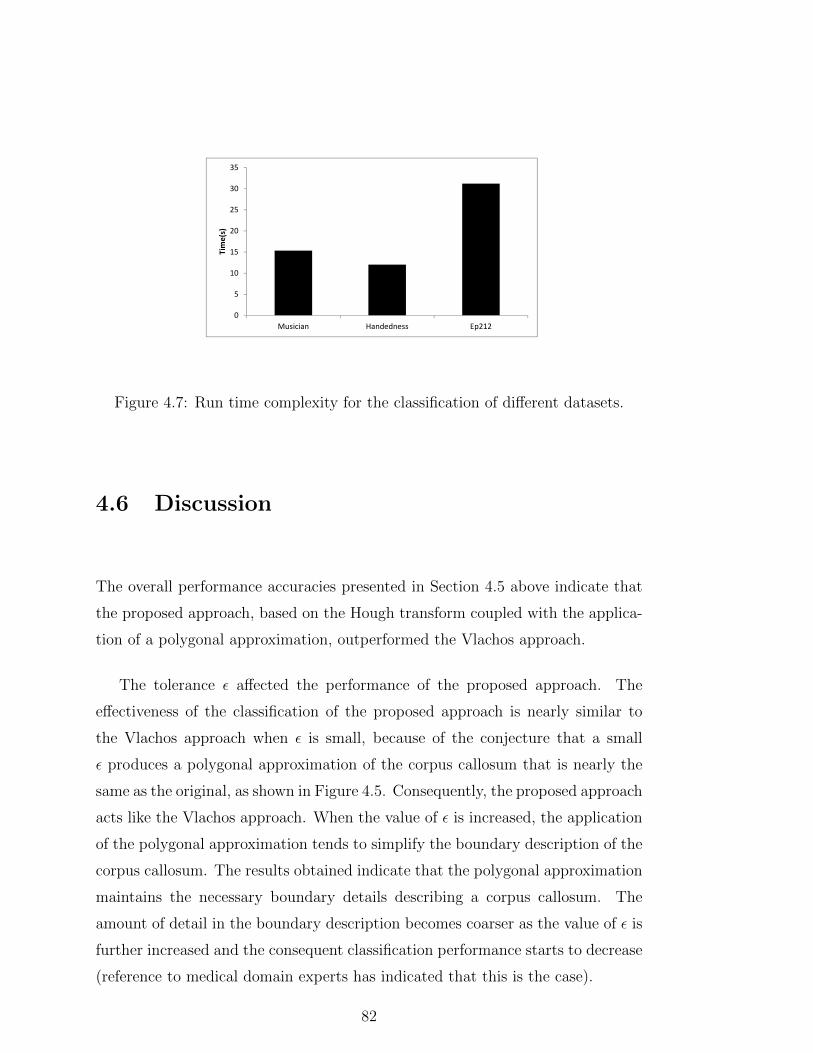
0
5
10
15
20
25
30
35
Musician Handedness Ep212
Tim
e(s)
Figure 4.7: Run time complexity for the classification of different datasets.
4.6 Discussion
The overall performance accuracies presented in Section 4.5 above indicate that
the proposed approach, based on the Hough transform coupled with the applica-
tion of a polygonal approximation, outperformed the Vlachos approach.
The tolerance ε affected the performance of the proposed approach. The
effectiveness of the classification of the proposed approach is nearly similar to
the Vlachos approach when ε is small, because of the conjecture that a small
ε produces a polygonal approximation of the corpus callosum that is nearly the
same as the original, as shown in Figure 4.5. Consequently, the proposed approach
acts like the Vlachos approach. When the value of ε is increased, the application
of the polygonal approximation tends to simplify the boundary description of the
corpus callosum. The results obtained indicate that the polygonal approximation
maintains the necessary boundary details describing a corpus callosum. The
amount of detail in the boundary description becomes coarser as the value of ε is
further increased and the consequent classification performance starts to decrease
(reference to medical domain experts has indicated that this is the case).
82
4.7 Summary
In this chapter a new approach to ROIBIC using the Hough transform, coupled
with a polygonal approximation, has been described. The Hough transform is a
popular technique used in image processing and analysis. Essentially it allows
the translation of an image into a higher dimension which in turn facilitates the
automated detection of objects. A number of variations of the Hough transform,
directed at different types of shape, were considered. The technique of interest
was that of Vlachos et al. which was used as the foundation for the proposed
Hough transform classification process. The distinction between the two tech-
niques is that the proposed technique adopted a polygonal approximation of the
region of interest. The reported evaluation indicated that the proposed technique
outperformed the Vlachos approach (which did not use any polygonal approxima-
tion). Reasonable classification results were obtained. However, in the following
Chapter an alternative approach to classifying images according to a common
image feature, founded on a tree representation, that outperforms the proposed
Hough transform technique will be described.
83

84
Chapter 5
Region Of Interest ImageClassification Using a WeightedFrequent SubgraphRepresentation
5.1 Introduction
As already noted, the application of techniques to classify image data according
to some common object that features across an image set requires the repre-
sentation of the image objects in question using some appropriate format. The
previous chapter consider representing image objects using a signature generation
process founded on the Hough transform. In this chapter an image decomposi-
tion method is considered whereby the ROIs are represented using a quad-tree
representation. More specifically the Minimum Bounding Rectangles (MBR) sur-
rounding the ROIs are represented using a quad-tree representation. The con-
jectured advantage offered is that a quad-tree representation will maintain the
structural information (shape and size) of the ROI contained in the MBR. By
applying a weighted frequent subgraph mining algorithm, gSpan-ATW [79], to
this representation, frequent subgraphs that occur across the tree represented set
of MBR can be identified. The identified frequent subgraphs each describing, in
terms of size and shape, some part of the MBR, can then be used to form the
fundamental elements of a feature space. Consequently, this feature space can
be used to describe a set of feature vectors, one per image, to which standard
classification processes can be applied (e.g. decision tree classifiers, SVM or rule
based classifiers). A schematic of the graph based approach is given in Figure
85
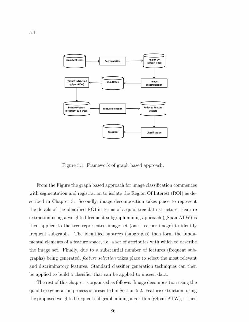
5.1.
Brain MRI scans SegmentationRegion Of
Interest (ROI)
Image
decompositionQuadtreesFeature Extraction
(gSpan-ATW)
Feature Vectors
(Frequent sub-trees)Feature Selection Reduced Feature
Vectors
ClassificationClassifier
Figure 5.1: Framework of graph based approach.
From the Figure the graph based approach for image classification commences
with segmentation and registration to isolate the Region Of Interest (ROI) as de-
scribed in Chapter 3. Secondly, image decomposition takes place to represent
the details of the identified ROI in terms of a quad-tree data structure. Feature
extraction using a weighted frequent subgraph mining approach (gSpan-ATW) is
then applied to the tree represented image set (one tree per image) to identify
frequent subgraphs. The identified subtrees (subgraphs) then form the funda-
mental elements of a feature space, i.e. a set of attributes with which to describe
the image set. Finally, due to a substantial number of features (frequent sub-
graphs) being generated, feature selection takes place to select the most relevant
and discriminatory features. Standard classifier generation techniques can then
be applied to build a classifier that can be applied to unseen data.
The rest of this chapter is organised as follows. Image decomposition using the
quad tree generation process is presented in Section 5.2. Feature extraction, using
the proposed weighted frequent subgraph mining algorithm (gSpan-ATW), is then
86
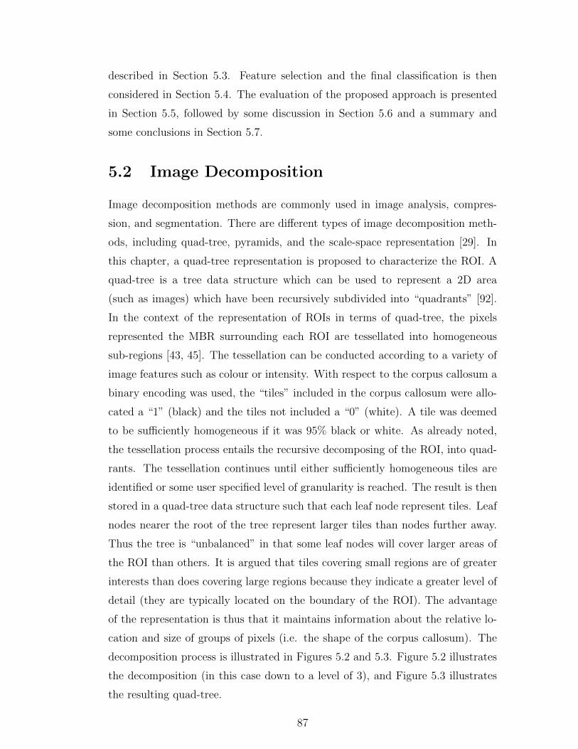
described in Section 5.3. Feature selection and the final classification is then
considered in Section 5.4. The evaluation of the proposed approach is presented
in Section 5.5, followed by some discussion in Section 5.6 and a summary and
some conclusions in Section 5.7.
5.2 Image Decomposition
Image decomposition methods are commonly used in image analysis, compres-
sion, and segmentation. There are different types of image decomposition meth-
ods, including quad-tree, pyramids, and the scale-space representation [29]. In
this chapter, a quad-tree representation is proposed to characterize the ROI. A
quad-tree is a tree data structure which can be used to represent a 2D area
(such as images) which have been recursively subdivided into “quadrants” [92].
In the context of the representation of ROIs in terms of quad-tree, the pixels
represented the MBR surrounding each ROI are tessellated into homogeneous
sub-regions [43, 45]. The tessellation can be conducted according to a variety of
image features such as colour or intensity. With respect to the corpus callosum a
binary encoding was used, the “tiles” included in the corpus callosum were allo-
cated a “1” (black) and the tiles not included a “0” (white). A tile was deemed
to be sufficiently homogeneous if it was 95% black or white. As already noted,
the tessellation process entails the recursive decomposing of the ROI, into quad-
rants. The tessellation continues until either sufficiently homogeneous tiles are
identified or some user specified level of granularity is reached. The result is then
stored in a quad-tree data structure such that each leaf node represent tiles. Leaf
nodes nearer the root of the tree represent larger tiles than nodes further away.
Thus the tree is “unbalanced” in that some leaf nodes will cover larger areas of
the ROI than others. It is argued that tiles covering small regions are of greater
interests than does covering large regions because they indicate a greater level of
detail (they are typically located on the boundary of the ROI). The advantage
of the representation is thus that it maintains information about the relative lo-
cation and size of groups of pixels (i.e. the shape of the corpus callosum). The
decomposition process is illustrated in Figures 5.2 and 5.3. Figure 5.2 illustrates
the decomposition (in this case down to a level of 3), and Figure 5.3 illustrates
the resulting quad-tree.
87
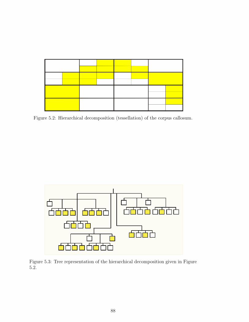
Figure 5.2: Hierarchical decomposition (tessellation) of the corpus callosum.
Figure 5.3: Tree representation of the hierarchical decomposition given in Figure5.2.
88
5.3 Feature Extraction Using gSpan-ATW Al-
gorithm
This section provides an overview of the weighted frequent subgraph mining algo-
rithm, gSpan-ATW, adopted for use with the quad-tree representation described
in Section 5.2. The section is divided into a number of sub-sections. Sub-section
5.3.1 first presents some necessary preliminary definitions. This is followed by
Sub-section 5.3.2 that presents an overview of frequent subgraph mining and
the gSpan algorithm on which gSpan-ATW is founded. The adopted weighted
frequent subgraph mining process is then described in Sub-section 5.3.3.
5.3.1 Definitions
The necessary definitions to support the discussion on frequent subgraph mining
presented in Sub-section 5.3.2 are introduced in this section. The definitions are
presented as follows.
Labelled Graph: A labelled graph can be represented as G(V,E, lV , lE, fV , fE),
where V is a set of nodes, E ⊆ V × V is a set of edges; lV and lE are node
and edge labels respectively, and fV and fE are the corresponding functions
that define the mappings V → lV and E → lE.
Subgraph: Given two graphsG1(V1, E1, lV1 , lE1 , fV1 , fE1) andG2(V2, E2, lV2 , lE2 , lV2 , lE2),
G1 is a subgraph of G2, if G1 satisfies the following conditions.
V1 ⊆ V2, ∀v ∈ V1, fV1(v) = fV2(v),
E1 ⊆ E2, ∀(u, v) ∈ E1, fE1(u, v) = fE2(u, v) .
G2 is also called a supergraph of G1 [76].
Graph Isomorphism: A graph G1(V1, E1, lV1 , lE1 , fV1 , fE1) is isomorphic to an-
other graph G2(V2, E2, lV2 , lE2 , fV2 , fE2), if and only if a bijection ψ : V1 → V2
exists such that:
∀u ∈ V1, fV1(u) = fV2(ψ(u)),
∀u, v ∈ V1, (u, v) ∈ E1 ⇔ (ψ(u), ψ(v)) ∈ E2,
∀(u, v) ∈ E1, fE1(u, v) = fE2(ψ(u), ψ(v)).
89
The bijection ψ is an isomorphism between G1 and G2. A graph G1 is
subgraph isomorphic to a graph G2, denoted by G1 ⊆sub G2, if and only if
there exists a subgraph g of G2 such that G1 is isomorphic to g [72].
5.3.2 Frequent Subgraph Mining
From the literature (see also Chapter 2) two separate problem formulations for
Frequent Subgraph Mining (FSM) can be identified: (i) transaction graph based,
and (ii) single graph based. In transaction graph based mining, the input data
comprises a collection of relatively small graphs, whereas in single graph based
mining the input data comprises a very large single graph. The graph mining
based approach described in this thesis focuses on transaction graph based mining.
Table 5.1 lists the notation, in relation to transaction graph based mining, which
will be employed through out the rest of this section (and where appropriate the
rest of this thesis).
Table 5.1: Notation used throughout this chapter.
Notation DescriptionD A graph database.Gi A transaction graph such that Gi ∈ D.k-(sub)graph A (sub)graph of size k in terms of nodes, or edges, or paths.gk A k-(sub)graph.Ck A set of subgraph candidates of size k .Fk A set of frequent k-subgraphs.| · | The cardinality of a set.
In the context of transaction graph based mining, FSM aims to discover all
the subgraphs whose occurrences in a graph database are over a user defined
threshold. Formally, given a database D comprised of a collection of graphs and
a threshold σ(0 < σ ≤ 1), the occurrence of a subgraph g in D is defined by
δD(g) = {Gi ∈ D|g ⊆sub Gi}. Thus, the support of a graph g is defined as the
fraction of the graphs in D to which g is subgraph isomorphic:
supD(g) = |δD(g)|/|D| (5.1)
A subgraph g is frequent if and only if supD(g) ≥ σ. The frequent sub-
graph mining problem is to find all the frequent subgraphs in D. Frequent
subgraph mining has been widely studied. A number of FSM algorithms have
90
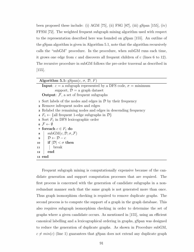
been proposed these include: (i) AGM [75], (ii) FSG [87], (iii) gSpan [155], (iv)
FFSM [72]. The weighted frequent subgraph mining algorithm used with respect
to the representation described here was founded on gSpan [155]. An outline of
the gSpan algorithm is given in Algorithm 5.1, note that the algorithm recursively
calls the “subGM” procedure. In the procedure, when subGM runs each time,
it grows one edge from c and discovers all frequent children of c (lines 6 to 12).
The recursive procedure in subGM follows the pre-order traversal as described in
[155].
Algorithm 5.1: gSpan(c, σ, D, F )
Input: c = a subgraph represented by a DFS code, σ = minimumsupport, D = a graph dataset
Output: F , a set of frequent subgraphs
1 Sort labels of the nodes and edges in D by their frequency2 Remove infrequent nodes and edges3 Relabel the remaining nodes and edges in descending frequency4 F1 ← {all frequent 1-edge subgraphs in D}5 Sort F1 in DFS lexicographic order6 F ← ∅7 foreach c ∈ F1 do8 subGM(c,D, σ,F)9 D ← D − c
10 if |D| < σ then11 break12 end
13 end
Frequent subgraph mining is computationally expensive because of the can-
didate generation and support computation processes that are required. The
first process is concerned with the generation of candidate subgraphs in a non-
redundant manner such that the same graph is not generated more than once.
Thus graph isomorphism checking is required to remove duplicate graphs. The
second process is to compute the support of a graph in the graph database. This
also requires subgraph isomorphism checking in order to determine the set of
graphs where a given candidate occurs. As mentioned in [155], using an efficient
canonical labelling and a lexicographical ordering in graphs, gSpan was designed
to reduce the generation of duplicate graphs. As shown in Procedure subGM,
c 6= min(c) (line 1) guarantees that gSpan does not extend any duplicate graph
91
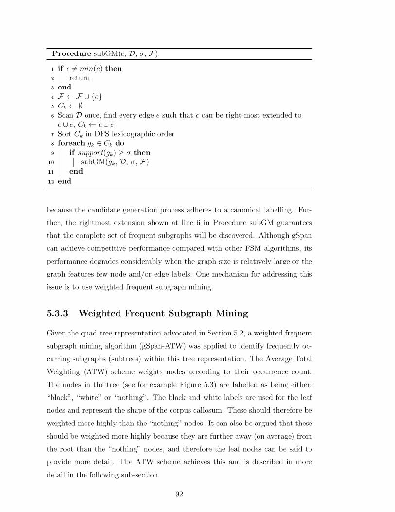
Procedure subGM(c, D, σ, F)
1 if c 6= min(c) then2 return3 end4 F ← F ∪ {c}5 Ck ← ∅6 Scan D once, find every edge e such that c can be right-most extended toc ∪ e, Ck ← c ∪ e
7 Sort Ck in DFS lexicographic order8 foreach gk ∈ Ck do9 if support(gk) ≥ σ then
10 subGM(gk, D, σ, F)11 end
12 end
because the candidate generation process adheres to a canonical labelling. Fur-
ther, the rightmost extension shown at line 6 in Procedure subGM guarantees
that the complete set of frequent subgraphs will be discovered. Although gSpan
can achieve competitive performance compared with other FSM algorithms, its
performance degrades considerably when the graph size is relatively large or the
graph features few node and/or edge labels. One mechanism for addressing this
issue is to use weighted frequent subgraph mining.
5.3.3 Weighted Frequent Subgraph Mining
Given the quad-tree representation advocated in Section 5.2, a weighted frequent
subgraph mining algorithm (gSpan-ATW) was applied to identify frequently oc-
curring subgraphs (subtrees) within this tree representation. The Average Total
Weighting (ATW) scheme weights nodes according to their occurrence count.
The nodes in the tree (see for example Figure 5.3) are labelled as being either:
“black”, “white” or “nothing”. The black and white labels are used for the leaf
nodes and represent the shape of the corpus callosum. These should therefore be
weighted more highly than the “nothing” nodes. It can also be argued that these
should be weighted more highly because they are further away (on average) from
the root than the “nothing” nodes, and therefore the leaf nodes can be said to
provide more detail. The ATW scheme achieves this and is described in more
detail in the following sub-section.
92
5.3.3.1 The Average Total Weighting (ATW) Scheme
The weighting scheme adopted in the gSpan-ATW algorithm is the Average Total
Weighting (ATW) scheme [79], which in turn is inspired by the work of [140].
Given a graph data set D = {G1, G2, · · · , Gt}, the weight for a subgraph g is
calculated by dividing the sum of the average weights in the graphs that contain
g with the sum of the average weights across the entire graph data set D. Thus:
Definition 5.3.1. Given a graph data set D = {G1, G2, · · · , Gt}, if Gi is node
weighted by assigning {w1, w2, · · · , wk} to a set of nodes {v1, v2, · · · , vk} respec-
tively, then the average weight associated with Gi is defined as:
Wavg(Gi) =
∑kj=1 wj
k. (5.2)
Where wj can be determined using an appropriate weighting function described
as follows:
wj =occ(vj)∑
1≤i≤t size(Gi). (5.3)
Where occ(vj) denotes the number of times vj occurs in D, and size(Gi) denotes
the size of Gi in terms of the number of nodes in Gi. Thus, the total weight of Dis further defined as:
Wsum(D) =t∑i=1
Wavg(Gi) . (5.4)
Using both (5.2) and (5.4), the weight of a subgraph can be calculated by (5.5).
Definition 5.3.2. Given a graph data set D = {G1, G2, · · ·Gt} and an arbitrary
subgraph g, let the set of graphs where g occurs equal δD(g). Then, the weight of
g with respect to D is:
WD(g) =
∑Gi∈δD(g) Wavg(Gi)
Wsum(D). (5.5)
WD(g) is used to quantify the actual importance of each discovered subgraph g
in a graph database. According to (5.1), the weighted support of a subgraph g is
then defined as the product of the support of g and the importance factor of g:
93
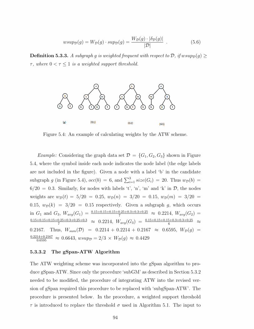
wsupD(g) = WD(g) · supD(g) =WD(g) · |δD(g)|
|D|. (5.6)
Definition 5.3.3. A subgraph g is weighted frequent with respect to D, if wsupD(g) ≥τ , where 0 < τ ≤ 1 is a weighted support threshold.
Figure 5.4: An example of calculating weights by the ATW scheme.
Example: Considering the graph data set D = {G1, G2, G3} shown in Figure
5.4, where the symbol inside each node indicates the node label (the edge labels
are not included in the figure). Given a node with a label ‘b’ in the candidate
subgraph g (in Figure 5.4), occ(b) = 6, and∑3
i=1 size(Gi) = 20. Thus wD(b) =
6/20 = 0.3. Similarly, for nodes with labels ‘t’, ‘n’, ‘m’ and ‘k’ in D, the nodes
weights are wD(t) = 5/20 = 0.25, wD(n) = 3/20 = 0.15, wD(m) = 3/20 =
0.15, wD(k) = 3/20 = 0.15 respectively. Given a subgraph g, which occurs
in G1 and G3, Wavg(G1) = 0.15+0.15+0.15+0.25+0.3+0.3+0.257
≈ 0.2214, Wavg(G2) =
0.15+0.15+0.15+0.25+0.3+0.25+0.37
≈ 0.2214, Wavg(G3) = 0.15+0.15+0.15+0.3+0.3+0.256
≈0.2167. Thus, Wsum(D) = 0.2214 + 0.2214 + 0.2167 ≈ 0.6595, WD(g) =
0.2214+0.21670.6595
≈ 0.6643, wsupD = 2/3 × WD(g) ≈ 0.4429
5.3.3.2 The gSpan-ATW Algorithm
The ATW weighting scheme was incorporated into the gSpan algorithm to pro-
duce gSpan-ATW. Since only the procedure ‘subGM’ as described in Section 5.3.2
needed to be modified, the procedure of integrating ATW into the revised ver-
sion of gSpan required this procedure to be replaced with ‘subgSpan-ATW’. The
procedure is presented below. In the procedure, a weighted support threshold
τ is introduced to replace the threshold σ used in Algorithm 5.1. The input to
94
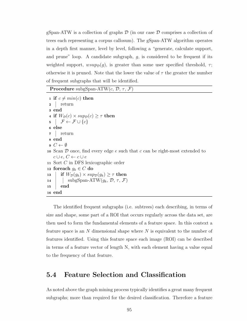
gSpan-ATW is a collection of graphs D (in our case D comprises a collection of
trees each representing a corpus callosum). The gSpan-ATW algorithm operates
in a depth first manner, level by level, following a “generate, calculate support,
and prune” loop. A candidate subgraph, g, is considered to be frequent if its
weighted support, wsupD(g), is greater than some user specified threshold, τ ;
otherwise it is pruned. Note that the lower the value of τ the greater the number
of frequent subgraphs that will be identified.
Procedure subgSpan-ATW(c, D, τ , F)
1 if c 6= min(c) then2 return3 end4 if WD(c)× supD(c) ≥ τ then5 F ← F ∪ {c}6 else7 return8 end9 C ← ∅
10 Scan D once, find every edge e such that c can be right-most extended toc ∪ e, C ← c ∪ e
11 Sort C in DFS lexicographic order12 foreach gk ∈ C do13 if WD(gk)× supD(gk) ≥ τ then14 subgSpan-ATW(gk, D, τ , F)15 end
16 end
The identified frequent subgraphs (i.e. subtrees) each describing, in terms of
size and shape, some part of a ROI that occurs regularly across the data set, are
then used to form the fundamental elements of a feature space. In this context a
feature space is an N dimensional shape where N is equivalent to the number of
features identified. Using this feature space each image (ROI) can be described
in terms of a feature vector of length N, with each element having a value equal
to the frequency of that feature.
5.4 Feature Selection and Classification
As noted above the graph mining process typically identifies a great many frequent
subgraphs; more than required for the desired classification. Therefore a feature
95
selection strategy was applied to the feature space so that only those subgraphs
that serve as good discriminators between cases are retained. A straightforward
wrapper method was adopted whereby a decision tree generator was applied to
the feature space. Features included as “choice points” in the decision tree were
then selected, while all remaining features were discarded. For the work described
here, the well established C4.5 algorithm [122] was adopted, although any other
decision tree generator would have sufficed. On completion of the feature selection
process each image was described in terms of a reduced feature vector indicating
the selected features (subgraphs) that appear in the image. Once the image set
had been represented in this manner any appropriate classifier generator could
be applied. With respect to the work described here two classification techniques
were used for the evaluation: (i) Decision Trees (C4.5) [122] and (ii) Support
Vector Machines (SVMs) [28], to examine the performance of the graph based
approach. For the C4.5 classifiers, the WEKA implementations [60] were used,
and for the SVM classifier, the LIBSVM implementation [22] was used. In the
experiments, all the classification results were computed using Ten-fold Cross
Validation (TCV).
5.5 Evaluation
The proposed graph based image classification approach was evaluated with re-
spect to the corpus callosum application. This section describes the evaluation.
The evaluation was undertaken in terms of classification accuracy, sensitivity and
specificity. The three studies introduced earlier were used for the evaluation: (i)
comparison between musician and non-musician MRI scans, (ii) comparison be-
tween left handedness and right handedness, and (iii) epilepsy screening. The
description of these datasets was presented in Chapter 3. The result of three
evaluations are discussed in detail in Sub-sections 5.5.1, 5.5.2 and 5.5.3 below.
The effect of the feature selection technique is considered in Subsection 5.5.4.
The run time analysis of the proposed approach is presented in Subsection 5.5.5
5.5.1 Musicians Study
For the musicians study four graph datasets were generated: QT-D4, QT-D5,
QT-D6, and QT-D7. These four datasets represent the same collection of brain
96
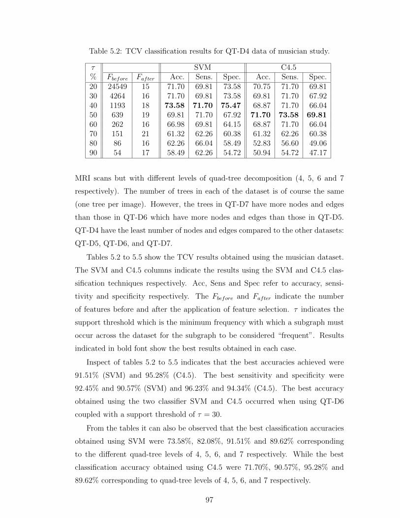
Table 5.2: TCV classification results for QT-D4 data of musician study.
τ SVM C4.5% Fbefore Fafter Acc. Sens. Spec. Acc. Sens. Spec.20 24549 15 71.70 69.81 73.58 70.75 71.70 69.8130 4264 16 71.70 69.81 73.58 69.81 71.70 67.9240 1193 18 73.58 71.70 75.47 68.87 71.70 66.0450 639 19 69.81 71.70 67.92 71.70 73.58 69.8160 262 16 66.98 69.81 64.15 68.87 71.70 66.0470 151 21 61.32 62.26 60.38 61.32 62.26 60.3880 86 16 62.26 66.04 58.49 52.83 56.60 49.0690 54 17 58.49 62.26 54.72 50.94 54.72 47.17
MRI scans but with different levels of quad-tree decomposition (4, 5, 6 and 7
respectively). The number of trees in each of the dataset is of course the same
(one tree per image). However, the trees in QT-D7 have more nodes and edges
than those in QT-D6 which have more nodes and edges than those in QT-D5.
QT-D4 have the least number of nodes and edges compared to the other datasets:
QT-D5, QT-D6, and QT-D7.
Tables 5.2 to 5.5 show the TCV results obtained using the musician dataset.
The SVM and C4.5 columns indicate the results using the SVM and C4.5 clas-
sification techniques respectively. Acc, Sens and Spec refer to accuracy, sensi-
tivity and specificity respectively. The Fbefore and Fafter indicate the number
of features before and after the application of feature selection. τ indicates the
support threshold which is the minimum frequency with which a subgraph must
occur across the dataset for the subgraph to be considered “frequent”. Results
indicated in bold font show the best results obtained in each case.
Inspect of tables 5.2 to 5.5 indicates that the best accuracies achieved were
91.51% (SVM) and 95.28% (C4.5). The best sensitivity and specificity were
92.45% and 90.57% (SVM) and 96.23% and 94.34% (C4.5). The best accuracy
obtained using the two classifier SVM and C4.5 occurred when using QT-D6
coupled with a support threshold of τ = 30.
From the tables it can also be observed that the best classification accuracies
obtained using SVM were 73.58%, 82.08%, 91.51% and 89.62% corresponding
to the different quad-tree levels of 4, 5, 6, and 7 respectively. While the best
classification accuracy obtained using C4.5 were 71.70%, 90.57%, 95.28% and
89.62% corresponding to quad-tree levels of 4, 5, 6, and 7 respectively.
97
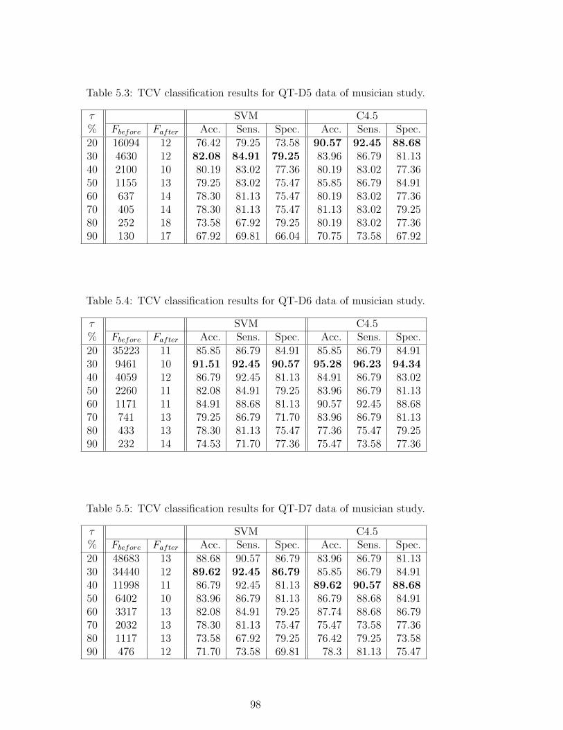
Table 5.3: TCV classification results for QT-D5 data of musician study.
τ SVM C4.5% Fbefore Fafter Acc. Sens. Spec. Acc. Sens. Spec.20 16094 12 76.42 79.25 73.58 90.57 92.45 88.6830 4630 12 82.08 84.91 79.25 83.96 86.79 81.1340 2100 10 80.19 83.02 77.36 80.19 83.02 77.3650 1155 13 79.25 83.02 75.47 85.85 86.79 84.9160 637 14 78.30 81.13 75.47 80.19 83.02 77.3670 405 14 78.30 81.13 75.47 81.13 83.02 79.2580 252 18 73.58 67.92 79.25 80.19 83.02 77.3690 130 17 67.92 69.81 66.04 70.75 73.58 67.92
Table 5.4: TCV classification results for QT-D6 data of musician study.
τ SVM C4.5% Fbefore Fafter Acc. Sens. Spec. Acc. Sens. Spec.20 35223 11 85.85 86.79 84.91 85.85 86.79 84.9130 9461 10 91.51 92.45 90.57 95.28 96.23 94.3440 4059 12 86.79 92.45 81.13 84.91 86.79 83.0250 2260 11 82.08 84.91 79.25 83.96 86.79 81.1360 1171 11 84.91 88.68 81.13 90.57 92.45 88.6870 741 13 79.25 86.79 71.70 83.96 86.79 81.1380 433 13 78.30 81.13 75.47 77.36 75.47 79.2590 232 14 74.53 71.70 77.36 75.47 73.58 77.36
Table 5.5: TCV classification results for QT-D7 data of musician study.
τ SVM C4.5% Fbefore Fafter Acc. Sens. Spec. Acc. Sens. Spec.20 48683 13 88.68 90.57 86.79 83.96 86.79 81.1330 34440 12 89.62 92.45 86.79 85.85 86.79 84.9140 11998 11 86.79 92.45 81.13 89.62 90.57 88.6850 6402 10 83.96 86.79 81.13 86.79 88.68 84.9160 3317 13 82.08 84.91 79.25 87.74 88.68 86.7970 2032 13 78.30 81.13 75.47 75.47 73.58 77.3680 1117 13 73.58 67.92 79.25 76.42 79.25 73.5890 476 12 71.70 73.58 69.81 78.3 81.13 75.47
98
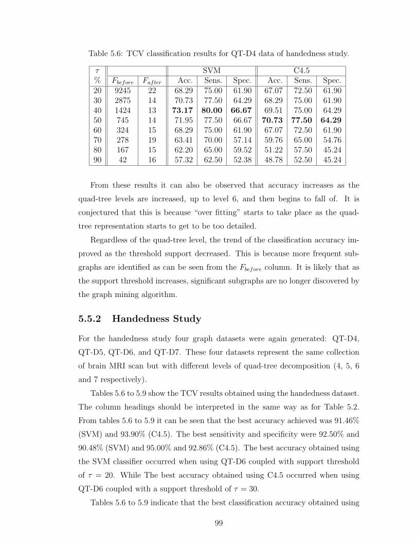
Table 5.6: TCV classification results for QT-D4 data of handedness study.
τ SVM C4.5% Fbefore Fafter Acc. Sens. Spec. Acc. Sens. Spec.20 9245 22 68.29 75.00 61.90 67.07 72.50 61.9030 2875 14 70.73 77.50 64.29 68.29 75.00 61.9040 1424 13 73.17 80.00 66.67 69.51 75.00 64.2950 745 14 71.95 77.50 66.67 70.73 77.50 64.2960 324 15 68.29 75.00 61.90 67.07 72.50 61.9070 278 19 63.41 70.00 57.14 59.76 65.00 54.7680 167 15 62.20 65.00 59.52 51.22 57.50 45.2490 42 16 57.32 62.50 52.38 48.78 52.50 45.24
From these results it can also be observed that accuracy increases as the
quad-tree levels are increased, up to level 6, and then begins to fall of. It is
conjectured that this is because “over fitting” starts to take place as the quad-
tree representation starts to get to be too detailed.
Regardless of the quad-tree level, the trend of the classification accuracy im-
proved as the threshold support decreased. This is because more frequent sub-
graphs are identified as can be seen from the Fbefore column. It is likely that as
the support threshold increases, significant subgraphs are no longer discovered by
the graph mining algorithm.
5.5.2 Handedness Study
For the handedness study four graph datasets were again generated: QT-D4,
QT-D5, QT-D6, and QT-D7. These four datasets represent the same collection
of brain MRI scan but with different levels of quad-tree decomposition (4, 5, 6
and 7 respectively).
Tables 5.6 to 5.9 show the TCV results obtained using the handedness dataset.
The column headings should be interpreted in the same way as for Table 5.2.
From tables 5.6 to 5.9 it can be seen that the best accuracy achieved was 91.46%
(SVM) and 93.90% (C4.5). The best sensitivity and specificity were 92.50% and
90.48% (SVM) and 95.00% and 92.86% (C4.5). The best accuracy obtained using
the SVM classifier occurred when using QT-D6 coupled with support threshold
of τ = 20. While The best accuracy obtained using C4.5 occurred when using
QT-D6 coupled with a support threshold of τ = 30.
Tables 5.6 to 5.9 indicate that the best classification accuracy obtained using
99
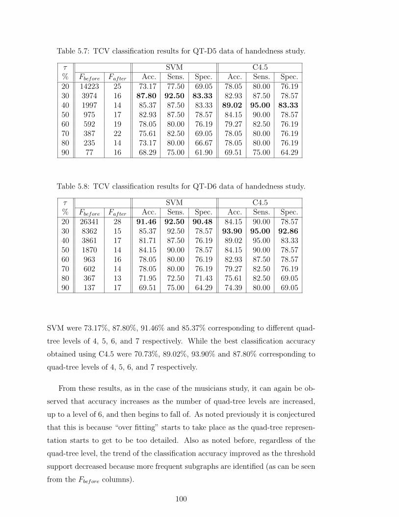
Table 5.7: TCV classification results for QT-D5 data of handedness study.
τ SVM C4.5% Fbefore Fafter Acc. Sens. Spec. Acc. Sens. Spec.20 14223 25 73.17 77.50 69.05 78.05 80.00 76.1930 3974 16 87.80 92.50 83.33 82.93 87.50 78.5740 1997 14 85.37 87.50 83.33 89.02 95.00 83.3350 975 17 82.93 87.50 78.57 84.15 90.00 78.5760 592 19 78.05 80.00 76.19 79.27 82.50 76.1970 387 22 75.61 82.50 69.05 78.05 80.00 76.1980 235 14 73.17 80.00 66.67 78.05 80.00 76.1990 77 16 68.29 75.00 61.90 69.51 75.00 64.29
Table 5.8: TCV classification results for QT-D6 data of handedness study.
τ SVM C4.5% Fbefore Fafter Acc. Sens. Spec. Acc. Sens. Spec.20 26341 28 91.46 92.50 90.48 84.15 90.00 78.5730 8362 15 85.37 92.50 78.57 93.90 95.00 92.8640 3861 17 81.71 87.50 76.19 89.02 95.00 83.3350 1870 14 84.15 90.00 78.57 84.15 90.00 78.5760 963 16 78.05 80.00 76.19 82.93 87.50 78.5770 602 14 78.05 80.00 76.19 79.27 82.50 76.1980 367 13 71.95 72.50 71.43 75.61 82.50 69.0590 137 17 69.51 75.00 64.29 74.39 80.00 69.05
SVM were 73.17%, 87.80%, 91.46% and 85.37% corresponding to different quad-
tree levels of 4, 5, 6, and 7 respectively. While the best classification accuracy
obtained using C4.5 were 70.73%, 89.02%, 93.90% and 87.80% corresponding to
quad-tree levels of 4, 5, 6, and 7 respectively.
From these results, as in the case of the musicians study, it can again be ob-
served that accuracy increases as the number of quad-tree levels are increased,
up to a level of 6, and then begins to fall of. As noted previously it is conjectured
that this is because “over fitting” starts to take place as the quad-tree represen-
tation starts to get to be too detailed. Also as noted before, regardless of the
quad-tree level, the trend of the classification accuracy improved as the threshold
support decreased because more frequent subgraphs are identified (as can be seen
from the Fbefore columns).
100
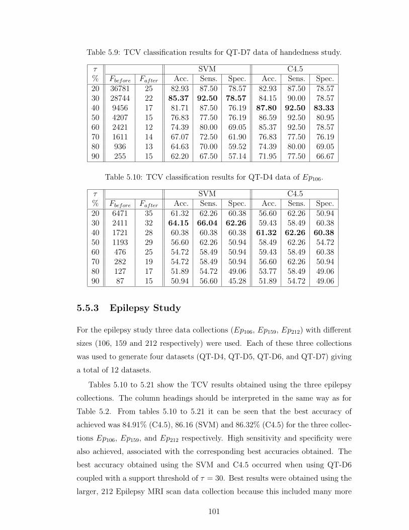
Table 5.9: TCV classification results for QT-D7 data of handedness study.
τ SVM C4.5% Fbefore Fafter Acc. Sens. Spec. Acc. Sens. Spec.20 36781 25 82.93 87.50 78.57 82.93 87.50 78.5730 28744 22 85.37 92.50 78.57 84.15 90.00 78.5740 9456 17 81.71 87.50 76.19 87.80 92.50 83.3350 4207 15 76.83 77.50 76.19 86.59 92.50 80.9560 2421 12 74.39 80.00 69.05 85.37 92.50 78.5770 1611 14 67.07 72.50 61.90 76.83 77.50 76.1980 936 13 64.63 70.00 59.52 74.39 80.00 69.0590 255 15 62.20 67.50 57.14 71.95 77.50 66.67
Table 5.10: TCV classification results for QT-D4 data of Ep106.
τ SVM C4.5% Fbefore Fafter Acc. Sens. Spec. Acc. Sens. Spec.20 6471 35 61.32 62.26 60.38 56.60 62.26 50.9430 2411 32 64.15 66.04 62.26 59.43 58.49 60.3840 1721 28 60.38 60.38 60.38 61.32 62.26 60.3850 1193 29 56.60 62.26 50.94 58.49 62.26 54.7260 476 25 54.72 58.49 50.94 59.43 58.49 60.3870 282 19 54.72 58.49 50.94 56.60 62.26 50.9480 127 17 51.89 54.72 49.06 53.77 58.49 49.0690 87 15 50.94 56.60 45.28 51.89 54.72 49.06
5.5.3 Epilepsy Study
For the epilepsy study three data collections (Ep106, Ep159, Ep212) with different
sizes (106, 159 and 212 respectively) were used. Each of these three collections
was used to generate four datasets (QT-D4, QT-D5, QT-D6, and QT-D7) giving
a total of 12 datasets.
Tables 5.10 to 5.21 show the TCV results obtained using the three epilepsy
collections. The column headings should be interpreted in the same way as for
Table 5.2. From tables 5.10 to 5.21 it can be seen that the best accuracy of
achieved was 84.91% (C4.5), 86.16 (SVM) and 86.32% (C4.5) for the three collec-
tions Ep106, Ep159, and Ep212 respectively. High sensitivity and specificity were
also achieved, associated with the corresponding best accuracies obtained. The
best accuracy obtained using the SVM and C4.5 occurred when using QT-D6
coupled with a support threshold of τ = 30. Best results were obtained using the
larger, 212 Epilepsy MRI scan data collection because this included many more
101
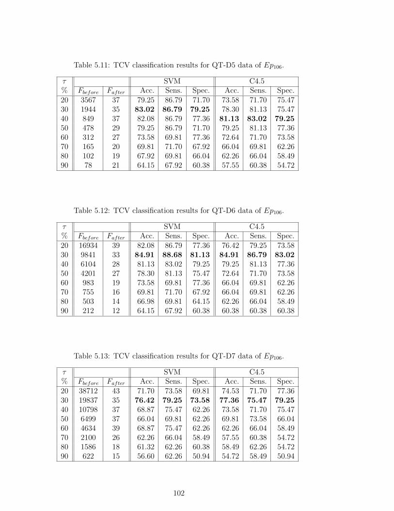
Table 5.11: TCV classification results for QT-D5 data of Ep106.
τ SVM C4.5% Fbefore Fafter Acc. Sens. Spec. Acc. Sens. Spec.20 3567 37 79.25 86.79 71.70 73.58 71.70 75.4730 1944 35 83.02 86.79 79.25 78.30 81.13 75.4740 849 37 82.08 86.79 77.36 81.13 83.02 79.2550 478 29 79.25 86.79 71.70 79.25 81.13 77.3660 312 27 73.58 69.81 77.36 72.64 71.70 73.5870 165 20 69.81 71.70 67.92 66.04 69.81 62.2680 102 19 67.92 69.81 66.04 62.26 66.04 58.4990 78 21 64.15 67.92 60.38 57.55 60.38 54.72
Table 5.12: TCV classification results for QT-D6 data of Ep106.
τ SVM C4.5% Fbefore Fafter Acc. Sens. Spec. Acc. Sens. Spec.20 16934 39 82.08 86.79 77.36 76.42 79.25 73.5830 9841 33 84.91 88.68 81.13 84.91 86.79 83.0240 6104 28 81.13 83.02 79.25 79.25 81.13 77.3650 4201 27 78.30 81.13 75.47 72.64 71.70 73.5860 983 19 73.58 69.81 77.36 66.04 69.81 62.2670 755 16 69.81 71.70 67.92 66.04 69.81 62.2680 503 14 66.98 69.81 64.15 62.26 66.04 58.4990 212 12 64.15 67.92 60.38 60.38 60.38 60.38
Table 5.13: TCV classification results for QT-D7 data of Ep106.
τ SVM C4.5% Fbefore Fafter Acc. Sens. Spec. Acc. Sens. Spec.20 38712 43 71.70 73.58 69.81 74.53 71.70 77.3630 19837 35 76.42 79.25 73.58 77.36 75.47 79.2540 10798 37 68.87 75.47 62.26 73.58 71.70 75.4750 6499 37 66.04 69.81 62.26 69.81 73.58 66.0460 4634 39 68.87 75.47 62.26 62.26 66.04 58.4970 2100 26 62.26 66.04 58.49 57.55 60.38 54.7280 1586 18 61.32 62.26 60.38 58.49 62.26 54.7290 622 15 56.60 62.26 50.94 54.72 58.49 50.94
102
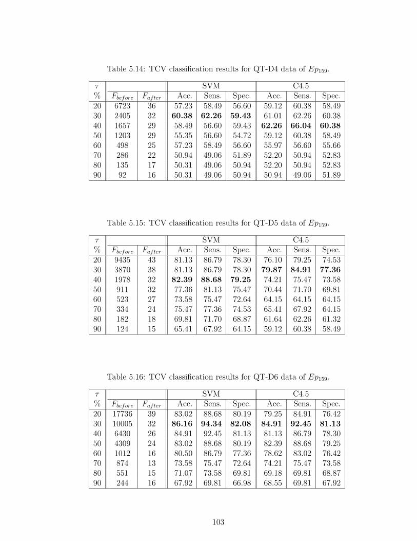
Table 5.14: TCV classification results for QT-D4 data of Ep159.
τ SVM C4.5% Fbefore Fafter Acc. Sens. Spec. Acc. Sens. Spec.20 6723 36 57.23 58.49 56.60 59.12 60.38 58.4930 2405 32 60.38 62.26 59.43 61.01 62.26 60.3840 1657 29 58.49 56.60 59.43 62.26 66.04 60.3850 1203 29 55.35 56.60 54.72 59.12 60.38 58.4960 498 25 57.23 58.49 56.60 55.97 56.60 55.6670 286 22 50.94 49.06 51.89 52.20 50.94 52.8380 135 17 50.31 49.06 50.94 52.20 50.94 52.8390 92 16 50.31 49.06 50.94 50.94 49.06 51.89
Table 5.15: TCV classification results for QT-D5 data of Ep159.
τ SVM C4.5% Fbefore Fafter Acc. Sens. Spec. Acc. Sens. Spec.20 9435 43 81.13 86.79 78.30 76.10 79.25 74.5330 3870 38 81.13 86.79 78.30 79.87 84.91 77.3640 1978 32 82.39 88.68 79.25 74.21 75.47 73.5850 911 32 77.36 81.13 75.47 70.44 71.70 69.8160 523 27 73.58 75.47 72.64 64.15 64.15 64.1570 334 24 75.47 77.36 74.53 65.41 67.92 64.1580 182 18 69.81 71.70 68.87 61.64 62.26 61.3290 124 15 65.41 67.92 64.15 59.12 60.38 58.49
Table 5.16: TCV classification results for QT-D6 data of Ep159.
τ SVM C4.5% Fbefore Fafter Acc. Sens. Spec. Acc. Sens. Spec.20 17736 39 83.02 88.68 80.19 79.25 84.91 76.4230 10005 32 86.16 94.34 82.08 84.91 92.45 81.1340 6430 26 84.91 92.45 81.13 81.13 86.79 78.3050 4309 24 83.02 88.68 80.19 82.39 88.68 79.2560 1012 16 80.50 86.79 77.36 78.62 83.02 76.4270 874 13 73.58 75.47 72.64 74.21 75.47 73.5880 551 15 71.07 73.58 69.81 69.18 69.81 68.8790 244 16 67.92 69.81 66.98 68.55 69.81 67.92
103
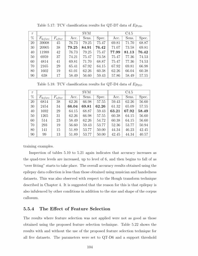
Table 5.17: TCV classification results for QT-D7 data of Ep159.
τ SVM C4.5% Fbefore Fafter Acc. Sens. Spec. Acc. Sens. Spec.20 39008 45 76.73 79.25 75.47 69.81 71.70 68.8730 20905 38 79.25 84.91 76.42 71.07 73.58 69.8140 11988 42 76.73 79.25 75.47 77.99 81.13 76.4250 6959 37 74.21 75.47 73.58 75.47 77.36 74.5360 4814 41 69.81 71.70 68.87 75.47 77.36 74.5370 2165 29 65.41 67.92 64.15 67.92 69.81 66.9880 1602 19 61.01 62.26 60.38 62.26 66.04 60.3890 638 17 58.49 56.60 59.43 57.86 58.49 57.55
Table 5.18: TCV classification results for QT-D4 data of Ep212.
τ SVM C4.5% Fbefore Fafter Acc. Sens. Spec. Acc. Sens. Spec.20 6814 38 62.26 66.98 57.55 59.43 62.26 56.6030 2454 34 66.04 69.81 62.26 61.32 65.09 57.5540 1692 29 64.15 68.87 59.43 63.21 67.92 58.4950 1265 31 62.26 66.98 57.55 60.38 64.15 56.6060 514 23 58.49 62.26 54.72 60.38 64.15 56.6070 293 19 56.60 59.43 53.77 52.36 53.77 50.9480 141 15 51.89 53.77 50.00 44.34 46.23 42.4590 99 13 51.89 53.77 50.00 42.45 44.34 40.57
training examples.
Inspection of tables 5.10 to 5.21 again indicates that accuracy increases as
the quad-tree levels are increased, up to level of 6, and then begins to fall of as
“over fitting” starts to take place. The overall accuracy results obtained using the
epilepsy data collection is less than those obtained using musician and handedness
datasets. This was also observed with respect to the Hough transform technique
described in Chapter 4. It is suggested that the reason for this is that epilepsy is
also infulenced by other conditions in addition to the size and shape of the corpus
callosum.
5.5.4 The Effect of Feature Selection
The results where feature selection was not applied were not as good as those
obtained using the proposed feature selection technique. Table 5.22 shows the
results with and without the use of the proposed feature selection technique for
all five datasets. The parameters were set to QT-D6 and a support threshold
104
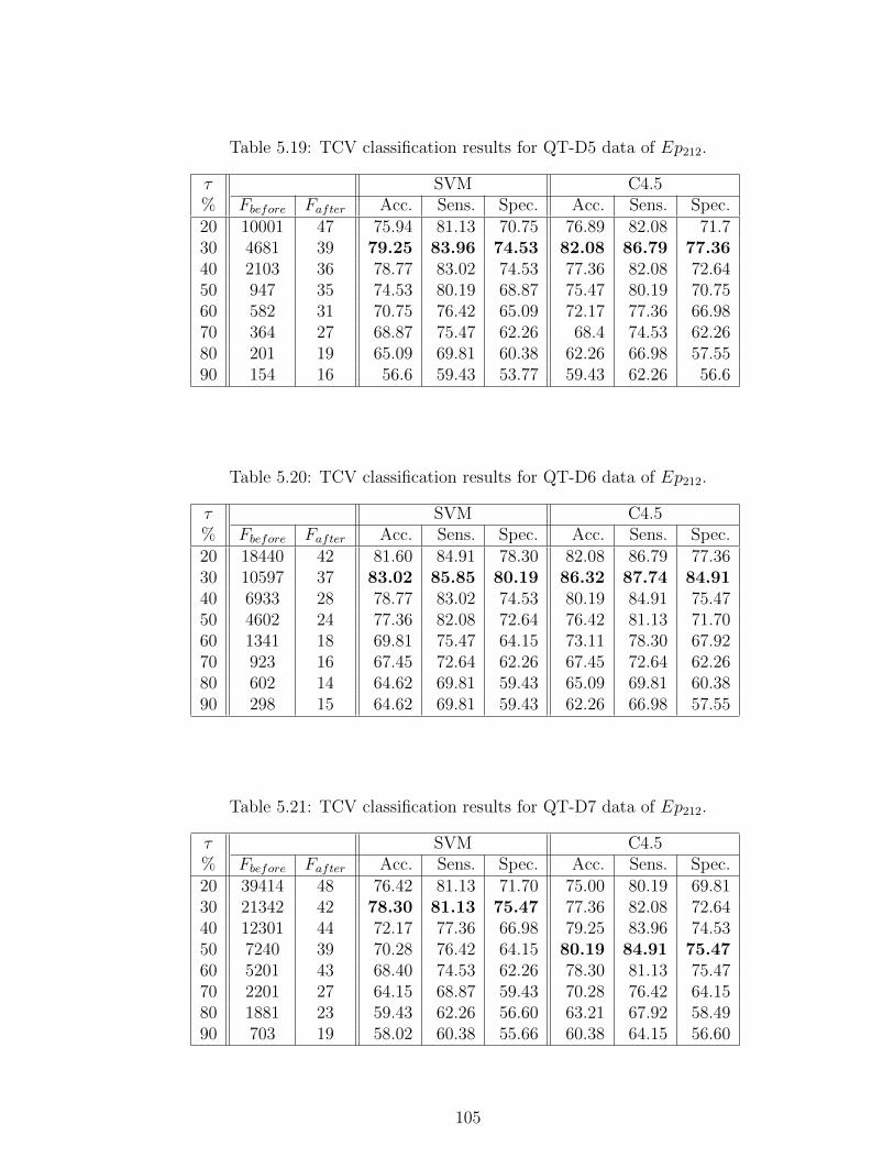
Table 5.19: TCV classification results for QT-D5 data of Ep212.
τ SVM C4.5% Fbefore Fafter Acc. Sens. Spec. Acc. Sens. Spec.20 10001 47 75.94 81.13 70.75 76.89 82.08 71.730 4681 39 79.25 83.96 74.53 82.08 86.79 77.3640 2103 36 78.77 83.02 74.53 77.36 82.08 72.6450 947 35 74.53 80.19 68.87 75.47 80.19 70.7560 582 31 70.75 76.42 65.09 72.17 77.36 66.9870 364 27 68.87 75.47 62.26 68.4 74.53 62.2680 201 19 65.09 69.81 60.38 62.26 66.98 57.5590 154 16 56.6 59.43 53.77 59.43 62.26 56.6
Table 5.20: TCV classification results for QT-D6 data of Ep212.
τ SVM C4.5% Fbefore Fafter Acc. Sens. Spec. Acc. Sens. Spec.20 18440 42 81.60 84.91 78.30 82.08 86.79 77.3630 10597 37 83.02 85.85 80.19 86.32 87.74 84.9140 6933 28 78.77 83.02 74.53 80.19 84.91 75.4750 4602 24 77.36 82.08 72.64 76.42 81.13 71.7060 1341 18 69.81 75.47 64.15 73.11 78.30 67.9270 923 16 67.45 72.64 62.26 67.45 72.64 62.2680 602 14 64.62 69.81 59.43 65.09 69.81 60.3890 298 15 64.62 69.81 59.43 62.26 66.98 57.55
Table 5.21: TCV classification results for QT-D7 data of Ep212.
τ SVM C4.5% Fbefore Fafter Acc. Sens. Spec. Acc. Sens. Spec.20 39414 48 76.42 81.13 71.70 75.00 80.19 69.8130 21342 42 78.30 81.13 75.47 77.36 82.08 72.6440 12301 44 72.17 77.36 66.98 79.25 83.96 74.5350 7240 39 70.28 76.42 64.15 80.19 84.91 75.4760 5201 43 68.40 74.53 62.26 78.30 81.13 75.4770 2201 27 64.15 68.87 59.43 70.28 76.42 64.1580 1881 23 59.43 62.26 56.60 63.21 67.92 58.4990 703 19 58.02 60.38 55.66 60.38 64.15 56.60
105
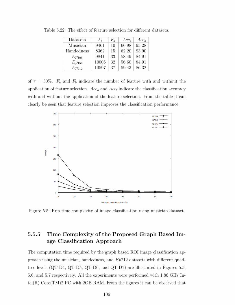
Table 5.22: The effect of feature selection for different datasets.
Datasets Fb Fa Accb AccaMusician 9461 10 66.98 95.28
Handedness 8362 15 62.20 93.90Ep106 9841 33 58.49 84.91Ep159 10005 32 56.60 84.91Ep212 10597 37 59.43 86.32
of τ = 30%. Fa and Fb indicate the number of feature with and without the
application of feature selection. Acca and Accb indicate the classification accuracy
with and without the application of the feature selection. From the table it can
clearly be seen that feature selection improves the classification performance.
Figure 5.5: Run time complexity of image classification using musician dataset.
5.5.5 Time Complexity of the Proposed Graph Based Im-age Classification Approach
The computation time required by the graph based ROI image classification ap-
proach using the musician, handedness, and Ep212 datasets with different quad-
tree levels (QT-D4, QT-D5, QT-D6, and QT-D7) are illustrated in Figures 5.5,
5.6, and 5.7 respectively. All the experiments were performed with 1.86 GHz In-
tel(R) Core(TM)2 PC with 2GB RAM. From the figures it can be observed that
106
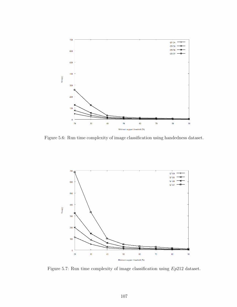
Figure 5.6: Run time complexity of image classification using handedness dataset.
Figure 5.7: Run time complexity of image classification using Ep212 dataset.
107
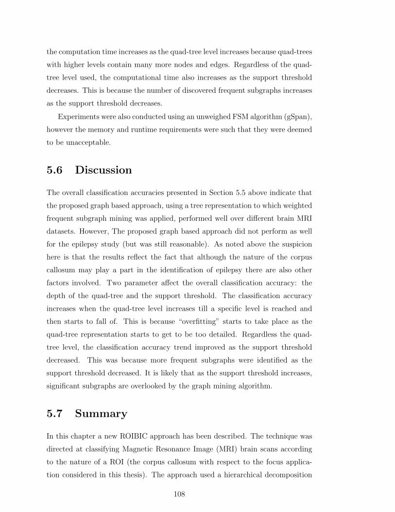
the computation time increases as the quad-tree level increases because quad-trees
with higher levels contain many more nodes and edges. Regardless of the quad-
tree level used, the computational time also increases as the support threshold
decreases. This is because the number of discovered frequent subgraphs increases
as the support threshold decreases.
Experiments were also conducted using an unweighed FSM algorithm (gSpan),
however the memory and runtime requirements were such that they were deemed
to be unacceptable.
5.6 Discussion
The overall classification accuracies presented in Section 5.5 above indicate that
the proposed graph based approach, using a tree representation to which weighted
frequent subgraph mining was applied, performed well over different brain MRI
datasets. However, The proposed graph based approach did not perform as well
for the epilepsy study (but was still reasonable). As noted above the suspicion
here is that the results reflect the fact that although the nature of the corpus
callosum may play a part in the identification of epilepsy there are also other
factors involved. Two parameter affect the overall classification accuracy: the
depth of the quad-tree and the support threshold. The classification accuracy
increases when the quad-tree level increases till a specific level is reached and
then starts to fall of. This is because “overfitting” starts to take place as the
quad-tree representation starts to get to be too detailed. Regardless the quad-
tree level, the classification accuracy trend improved as the support threshold
decreased. This was because more frequent subgraphs were identified as the
support threshold decreased. It is likely that as the support threshold increases,
significant subgraphs are overlooked by the graph mining algorithm.
5.7 Summary
In this chapter a new ROIBIC approach has been described. The technique was
directed at classifying Magnetic Resonance Image (MRI) brain scans according
to the nature of a ROI (the corpus callosum with respect to the focus applica-
tion considered in this thesis). The approach used a hierarchical decomposition
108
whereby each MRI scan was decomposed into a hierarchy of “tiles” which could
then be represented as a quad-tree structure (one quad-tree per scan). A weighted
frequent subgraph mining mechanism was then applied so that subgraphs that
occurred frequently across the image set could be identified. These frequent sub-
graphs could be viewed as describing a feature space; as such the input images
could be translated, according to this feature space, into a set of feature vec-
tors (one per image). A feature selection mechanism was applied to the feature
vectors so as to select the most significant features to which standard classifica-
tion techniques could be applied. The reported evaluation indicates that high
classification accuracy results were obtained when using higher quad-tree levels
of decomposition, coupled with low support threshold, although if the level of
decomposition gets too high “over fitting” starts to take place. In the following
chapter an alternative approach for classifying images according to a common
image feature, founded on Zernike moments, is described.
109

110
Chapter 6
Region Of Interest ImageClassification Using a ZernikeMoment SignatureRepresentation
6.1 Introduction
Moments are scalar quantities used to characterize a function and to capture
its significant features. They have been widely used for hundreds of years in
statistics for the description of the shape of probability density functions and in
classic “rigid-body” mechanics to measure the mass distribution of a body. From
the mathematical point of view, moments are “projections” of a function onto a
polynomial basis. The general moment Gpq of an image function f(x, y), where
p, q are non-negative integers and r = p + q is called the order of the moment,
defined as:
Gpq =
∫∫D
Ppq(x, y) f(x, y) dx dy, (6.1)
where P00(x, y), P10(x, y), ..., Pkj(x, y), ... are polynomial basis functions defined
on D. Depending on the polynomial basis used, various systems of moments may
be defined. The most common is a standard power basis Pkj(x, y) = xkyj that
leads to geometric moments, Mpq:
Mpq =
∞∫−∞
∞∫−∞
xpyqf(x, y) dx dy. (6.2)
Geometric moments of low orders have an intuitive meaning - M00 is a “mass” of
the image (for binary images, M00 is an area of the object), M10/M00 andM01/M00
111
define the centroid of the image. Another popular choice of the polynomial basis
Pkj(x, y) = (x+ iy)k(x− iy)j, where i =√−1, leads to complex moments, Cpq:
Cpq =
∞∫−∞
∞∫−∞
(x+ iy)p (x− iy)q f(x, y) dx dy. (6.3)
If the polynomial basis {Pkj(x, y)} is orthogonal, i.e. if its elements satisfy
the condition of orthogonality for any indexes p 6= m or q 6= n then:∫∫D
Ppq(x, y).Pmn(x, y) dx dy = 0 (6.4)
The advantage of orthogonal moments is their ability to capture the image fea-
tures in an improved, nonredundant way. Zernike moments are a class of orthogo-
nal moments (moments produced using orthogonal basis sets) that can be used as
an effective image descriptor. Zernike moments were first introduced by Teague
[141]. Teh and Chin [142] evaluated various image moments in terms of their
image description capabilities and noise sensitivity, The evaluation included: (i)
geometric, (ii) Legendre, (iii) Zernike, (iv) pseudo-Zernike, (v) rotational, and
(vi) complex moments. They showed that Zernike moments outperformed the
other moments. Unfortunately, direct computation of Zernike moments from
the Zernike polynomial is computationally expensive. This makes it impracti-
cal for many applications. This limitation has prompted considerable study of
algorithms for fast evaluation of Zernike moments [15, 86, 105, 119]. Several
algorithms have been proposed to speed up the computation. Belkasim et al.
[15] introduced a fast algorithm based on the series expansion of radial polyno-
mials. Parta et al. [119] and Kintner [86] have proposed recurrence relations
for fast computation of radial polynomials of Zernike moments. However, these
techniques are not applicable in many cases for the computation of Zernike mo-
ments where ((p = q) and (q = 0)), and (p − q < 4) respectively. Chong et
al. [23] modified Kintners method so that it would be applicable for all cases.
Unfortunately, all of these methods approximated Zernike moment polynomials
and consequently, produced inaccurate sets of Zernike moments. On the other
hand, Wee et al. [150], proposed a new algorithm that computed exact Zernike
moments through a set of exact geometric moments. Their method is accurate,
but it is time consuming. In this chapter, we introduce a new method for ex-
act Zernike Moment computation based on the observation that exact Zernike
112
moments can be expressed as a function of geometric moments. Wu et al. [152]
describe a fast algorithm that accelerates the computation of geometric moments.
The algorithm is based on a quad-tree representation of images (similar to that
described in Chapter 5) whereby a given pixel represented region is decomposed
into a number of non-overlapping tiles. Since the geometric moment computation
for each tile is easier than that for the whole region, the algorithm proposed by
Wu reduces the computational complexity significantly.
In this chapter a mechanism for fast Zernike moment calculation, based on the
work of Wu [152], is proposed. The resulting Zernike moments are used to define
a feature vector (one per image) which can be input to a standard classification
mechanism (a SVM and C4.5 were used for evaluation). The rest of this chapter
is organized as follows. In Section 6.2 a review of Zernike moments is presented in
terms of their general application to image analysis. In Section 6.3 the calculation
of Zernike moments in terms of geometric moments is presented. Section 6.4
then presents a mechanism, first proposed in [152], for the fast calculation of
geometric moments using the quad-tree decomposition. The proposed mechanism
for the fast calculation of Zernike moments is presented in Section 6.5. In Section
6.6 feature extraction based on Zernike moments, to support ROI based image
classification, is introduced. The evaluation of the proposed approach is presented
in Section 6.7. Finally, Some discussion and summary is then presented in Section
6.8.
6.2 Zernike Moments
The complex 2D Zernike moments of order p and repetition q of an image intensity
function f(r, θ) are defined as:
Zpq =p+ 1
π
∫ 2π
0
∫ 1
0
[Vpq(r, θ)
]∗f(r, θ) r dr dθ (6.5)
where p = 0, 1, 2, ...,∞ and q is an integer such that p− |q| = even, |q| ≤ p. * is
the complex conjugate. The p-th order Zernike polynomials with repetition q are
defined as:
Vpq(r, θ) = Rpq(r)eiqθ (6.6)
113
where r =√x2 + y2, r ∈ [−1, 1] is the length of the vector from the image
pixel (x, y) to the origin, θ = arctan(y/x) is the angle between vector r and the
principle x-axis and i =√−1. These Zernike polynomials describe a complete
set of complex-valued orthogonal functions defined on the unit circle, x2 +y2 ≤ 1.
The real-valued radial polynomials Rpq(r) are defined as:
Rpq(r) =
p∑k=q
p−k=even
Bp|q|krk (6.7)
where the polynomial coefficients, Bp|q|k, are defined as:
Bp|q|k =
(−1)
(p− k
2
)(p+ k
2
)!(
p− k2
)!
(k + q
2
)!
(k − q
2
)!
(6.8)
The Zernike polynomial coefficients can be computed using the recurrent re-
lations proposed in [105] as follows:
Bppp = 1
Bp(q−2)p =p+ q
p− q + 2Bpqp
Bpq(k−2) = − (k + q)(k − q)(p+ k)(p− k + 2)
Bpqk (6.9)
Zernike polynomials satisfy the orthogonality relationship:
2π∫0
1∫0
Vnm(r, θ)Vpq(r, θ) r dr dθ =
{πp+1
, p = n, q = m
0, otherwise(6.10)
Zernike moments are by nature rotation invariant, therefore the magnitudes
of Zernike moments are unaffected and remain constant with respect to an image
function regardless of any rotation. If an image function f(r, θ) with a Zernike
moment Zpq is rotated counter-clockwise by angle α, the transformed image func-
tion is g(r, θ) = f(r, θ − α). The Zernike moment of the rotated image is given
by:
Zαpq = e−iqαZpq. (6.11)
114
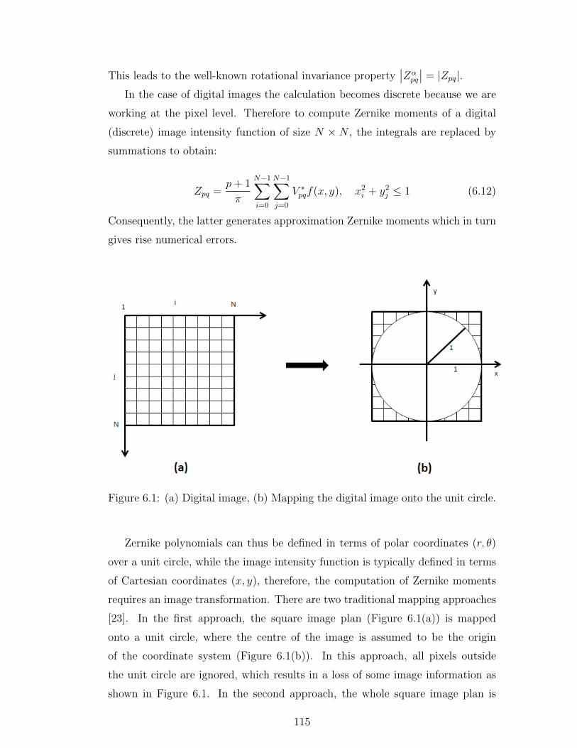
This leads to the well-known rotational invariance property∣∣Zα
pq
∣∣ = |Zpq|.In the case of digital images the calculation becomes discrete because we are
working at the pixel level. Therefore to compute Zernike moments of a digital
(discrete) image intensity function of size N × N , the integrals are replaced by
summations to obtain:
Zpq =p+ 1
π
N−1∑i=0
N−1∑j=0
V ∗pqf(x, y), x2i + y2
j ≤ 1 (6.12)
Consequently, the latter generates approximation Zernike moments which in turn
gives rise numerical errors.
Figure 6.1: (a) Digital image, (b) Mapping the digital image onto the unit circle.
Zernike polynomials can thus be defined in terms of polar coordinates (r, θ)
over a unit circle, while the image intensity function is typically defined in terms
of Cartesian coordinates (x, y), therefore, the computation of Zernike moments
requires an image transformation. There are two traditional mapping approaches
[23]. In the first approach, the square image plan (Figure 6.1(a)) is mapped
onto a unit circle, where the centre of the image is assumed to be the origin
of the coordinate system (Figure 6.1(b)). In this approach, all pixels outside
the unit circle are ignored, which results in a loss of some image information as
shown in Figure 6.1. In the second approach, the whole square image plan is
115
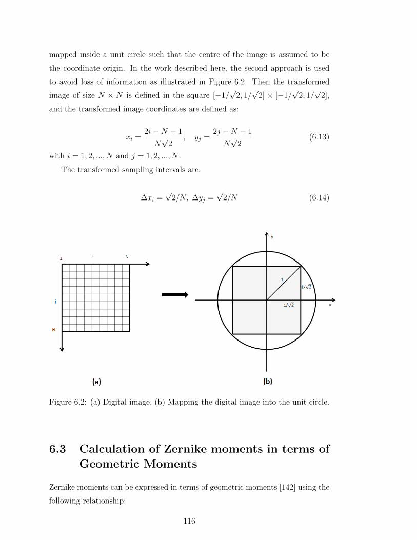
mapped inside a unit circle such that the centre of the image is assumed to be
the coordinate origin. In the work described here, the second approach is used
to avoid loss of information as illustrated in Figure 6.2. Then the transformed
image of size N × N is defined in the square [−1/√
2, 1/√
2] × [−1/√
2, 1/√
2],
and the transformed image coordinates are defined as:
xi =2i−N − 1
N√
2, yj =
2j −N − 1
N√
2(6.13)
with i = 1, 2, ..., N and j = 1, 2, ..., N .
The transformed sampling intervals are:
∆xi =√
2/N, ∆yj =√
2/N (6.14)
Figure 6.2: (a) Digital image, (b) Mapping the digital image into the unit circle.
6.3 Calculation of Zernike moments in terms of
Geometric Moments
Zernike moments can be expressed in terms of geometric moments [142] using the
following relationship:
116
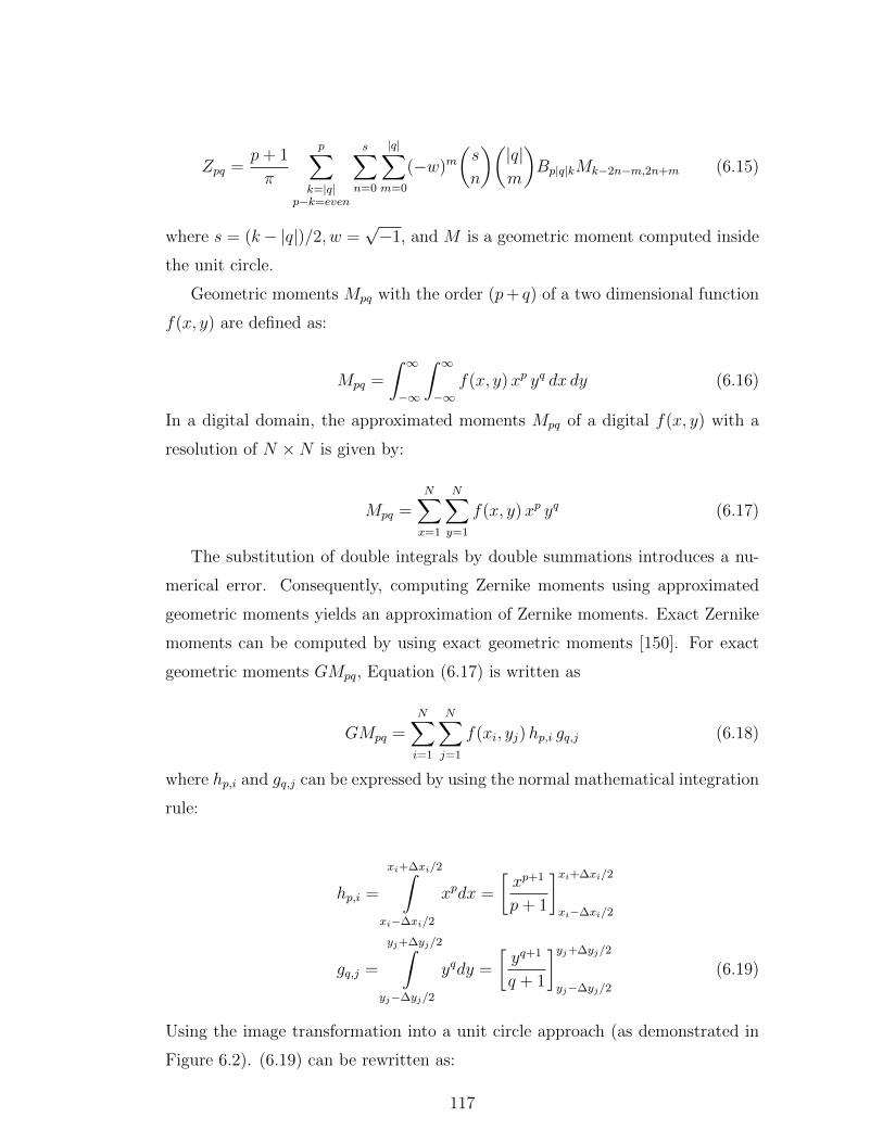
Zpq =p+ 1
π
p∑k=|q|
p−k=even
s∑n=0
|q|∑m=0
(−w)m(s
n
)(|q|m
)Bp|q|kMk−2n−m,2n+m (6.15)
where s = (k− |q|)/2, w =√−1, and M is a geometric moment computed inside
the unit circle.
Geometric moments Mpq with the order (p+ q) of a two dimensional function
f(x, y) are defined as:
Mpq =
∫ ∞−∞
∫ ∞−∞
f(x, y)xp yq dx dy (6.16)
In a digital domain, the approximated moments Mpq of a digital f(x, y) with a
resolution of N ×N is given by:
Mpq =N∑x=1
N∑y=1
f(x, y)xp yq (6.17)
The substitution of double integrals by double summations introduces a nu-
merical error. Consequently, computing Zernike moments using approximated
geometric moments yields an approximation of Zernike moments. Exact Zernike
moments can be computed by using exact geometric moments [150]. For exact
geometric moments GMpq, Equation (6.17) is written as
GMpq =N∑i=1
N∑j=1
f(xi, yj)hp,i gq,j (6.18)
where hp,i and gq,j can be expressed by using the normal mathematical integration
rule:
hp,i =
xi+∆xi/2∫xi−∆xi/2
xpdx =
[xp+1
p+ 1
]xi+∆xi/2
xi−∆xi/2
gq,j =
yj+∆yj/2∫yj−∆yj/2
yqdy =
[yq+1
q + 1
]yj+∆yj/2
yj−∆yj/2
(6.19)
Using the image transformation into a unit circle approach (as demonstrated in
Figure 6.2). (6.19) can be rewritten as:
117
hp,i =
[Up+1i+1 − U
p+1i
p+ 1
]
gq,j =
[U q+1j+1 − U
q+1j
q + 1
](6.20)
with
Ui+1 =2i−NN√
2
Ui =2(i− 1)−N
N√
2(6.21)
Then the numerical error introduced by replacing the double integrals with
double summations can be eliminated by calculating exact Zernike moments in
terms of exact geometric moments. Thus:
Zpq =p+ 1
π
p∑k=|q|
p−k=even
s∑n=0
|q|∑m=0
(−w)m(s
n
)(|q|m
)Bp|q|kGMk−2n−m,2n+m (6.22)
Therefore the above mechanism was adopted for use with the ROIBIC method
suggested in this chapter. On the other hand, computation of exact geometric
moments as described above is time consuming. Therefore, in the next section,
a method to speed up this computation is described.
6.4 Fast Calculation of Geometric Moments
To speed up the calculation of Zernike moments in terms of geometric moments
as described in the foregoing, we use a quad-tree decomposition similar to that
used in the graph based approach described in Chapter 5. Wu et al. [152] also
proposed using the quad-tree decomposition as the first stage of their geometric
moment computation method. The decomposition operates using square images,
ideally with a size of power of two. The image is iteratively divided into four
quadrants (tiles). The homogeneity of each quadrants is checked and if the whole
quadrants lies either in the region or in the background, it is not further divided. If
118
it contains both region and background pixels it is divided into further quadrants
and the process is repeated until all tiles are homogeneous.
After the decomposition, the ROI will be represented by a quad-tree of k
non-overlapping square tiles B1, B2, ..., Bk. Then the computational complexity
of the geometric moments can be decreased by computing the geometric moments
of these k tiles. For each tile Bi, the coordinate indices of its upper left corner
are (a, b) and the length of tile side is w. The geometric moments GMpq,i for the
block Bi can then be calculated using equations 6.18, 6.19 and 6.20, as:
GMpq,i =
xa+w−1+ ∆x2∫
xa−∆x2
xpdx
yb+w−1+ ∆y2∫
yb−∆y2
yqdy
=
[Up+1
2 − Up+11
p+ 1
] [U q+1
4 − U q+13
q + 1
](6.23)
with:
U1 =2(a− 1)−N
N√
2
U2 =2(a+ w − 2)−N
N√
2
U3 =2(b− 1)−N
N√
2
U4 =2(b+ w − 2)−N
N√
2(6.24)
Then, the geometric moment of the ROI can be easily calculated by summing
the geometric moments of all k tiles in the decomposition that are part of the
ROI, since the computation of geometric moments of tiles is easier than that for
the whole ROI where k < N2. Then, the geometric moment for the entire ROI
can be calculated as follows:
GMpq =k∑
n=1
GMpq,n (6.25)
In the work described here the decomposition is conducted down to the pixel
level (unlike in the case of the quad-tree decomposition described in Chapter 5).
Also the homogeneity condition, unlike previously, is 100% black or white. This
119
is to ensure that exact geometric moments are derived. Note that if the image is
entirely decomposed down to the pixel level (e.g. if we have a “checker board”
image) then the method will be similar to the Wee method [150].
6.5 Fast Calculation of Zernike Moments
The proposed mechanism for the fast calculation of Zernike moments adopts
the idea of representing the exact Zernike moments in terms of exact geometric
moments calculated using a quad-tree decomposition of the form described above.
This decomposition is used to speed up the computation of geometric moments as
also described above. The procedure for computing a full set of Zernike moments
is as follows (here Max is the maximum order of moments to be calculated):
1. Transform the image (or a ROI) into a unit circle so that the transformed
image of size N×N is defined in the square [−1/√
2, 1/√
2]×[−1/√
2, 1/√
2].
2. Decompose the image into k square tiles, B1, B2, ..., Bk, using a quad-tree
decomposition as described in Section 6.4.
3. For p=0 to Max
Compute the Zernike polynomial coefficients B as in Eq. (6.9).
4. For p=0 to Max & q=0 to Max
Compute GMpq using Eq. (6.23), (6.24), (6.25)
5. For p=0 to Max & For q=0 to p
Compute Zpq using Eq. (6.22).
The Zernike moment magnitudes thus calculated is then used to define a feature
space for each image (or ROI).
6.6 Feature Extraction Based on Zernike Mo-
ments
In the context of the proposed ROIBIC approach, the Zernike moment mag-
nitudes are used to define a feature space representing the image set. Each
image, or more specifically the object of interest within each image, can then
120
be represented in terms of a feature vector. The feature vector {AFV }N will
then consist of the accumulated Zernike moment magnitudes from order p = 0
to order p = N with all possible repetitions q. For example, where N = 4,
the feature vector {AFV }4 will consist of the set of all Zernike moments cor-
responding to the orders p = 0, 1, 2, 3, 4 coupled with all possible repetitions q:
{|Z00|, |Z11|, |Z20|, |Z22|, |Z31|, |Z33|, |Z40| , |Z42|, |Z44|}.Consequently a set of images that contain a common ROI (such as the corpus
callosum in the case of the brain MRI scan data of interest with respect to this
thesis) can be represented as a set of feature vectors which can be input to
standard classification techniques.
6.7 Evaluation
This evaluation section is divided into four subsections: (i) experimental studies
on the validity of the proposed method of Zernike moments computation, (ii)
speed of the calculation of Zernike moments according to the proposed approach,
(iii) the evaluation of using Zernike moments in the context of image classification,
and (iv) run time analysis of the proposed classification technique.
6.7.1 Experimental Studies on the Validity of the Pro-posed Method of Zernike Moments Computation
An artificial image were used to demonstrate the validity of the proposed method.
The artificial image used was a 4 × 4 pixel image in which all pixel intensity
values were one, f(x, y) = 1 for all pixels (x, y). The image defined in the square
[−1, 1] × [−1, 1] was mapped to be inside the unit circle where the coordinate
origin was the center of the circle. The mapped image was defined in the square
[−1/√
2, 1/√
2] × [−1/√
2, 1/√
2]. The theoretical values of the exact Zernike
moments, ZTheopq , were then computed using:
ZTheopq =
p+ 1
π
p∑k=q
p−k=even
Bpqk
s∑n=0
(s
n
) |q|∑m=0
(−w)m(q
m
)∫ 1√2
−1√2
x(k−2n+m) dx
∫ 1√2
−1√2
y(2n+m) dy
(6.26)
where s = (k − q)/2 and w =√−1. The approximated Zernike moments Zapprox
pq
were calculated using Equations (6.15),(6.17) while the proposed exact Zernike
121
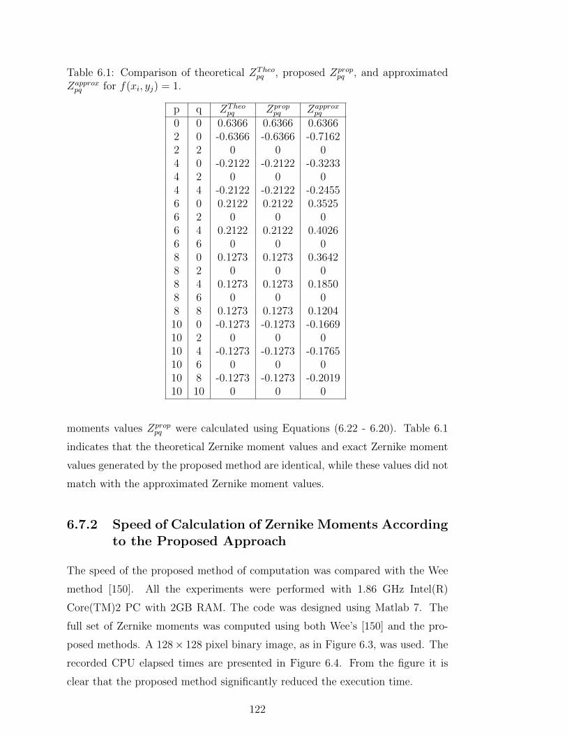
Table 6.1: Comparison of theoretical ZTheopq , proposed Zprop
pq , and approximatedZapproxpq for f(xi, yj) = 1.
p q ZTheopq Zprop
pq Zapproxpq
0 0 0.6366 0.6366 0.63662 0 -0.6366 -0.6366 -0.71622 2 0 0 04 0 -0.2122 -0.2122 -0.32334 2 0 0 04 4 -0.2122 -0.2122 -0.24556 0 0.2122 0.2122 0.35256 2 0 0 06 4 0.2122 0.2122 0.40266 6 0 0 08 0 0.1273 0.1273 0.36428 2 0 0 08 4 0.1273 0.1273 0.18508 6 0 0 08 8 0.1273 0.1273 0.120410 0 -0.1273 -0.1273 -0.166910 2 0 0 010 4 -0.1273 -0.1273 -0.176510 6 0 0 010 8 -0.1273 -0.1273 -0.201910 10 0 0 0
moments values Zproppq were calculated using Equations (6.22 - 6.20). Table 6.1
indicates that the theoretical Zernike moment values and exact Zernike moment
values generated by the proposed method are identical, while these values did not
match with the approximated Zernike moment values.
6.7.2 Speed of Calculation of Zernike Moments Accordingto the Proposed Approach
The speed of the proposed method of computation was compared with the Wee
method [150]. All the experiments were performed with 1.86 GHz Intel(R)
Core(TM)2 PC with 2GB RAM. The code was designed using Matlab 7. The
full set of Zernike moments was computed using both Wee’s [150] and the pro-
posed methods. A 128× 128 pixel binary image, as in Figure 6.3, was used. The
recorded CPU elapsed times are presented in Figure 6.4. From the figure it is
clear that the proposed method significantly reduced the execution time.
122
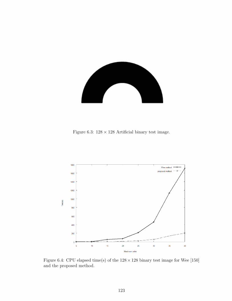
Figure 6.3: 128× 128 Artificial binary test image.
Figure 6.4: CPU elapsed time(s) of the 128×128 binary test image for Wee [150]and the proposed method.
123
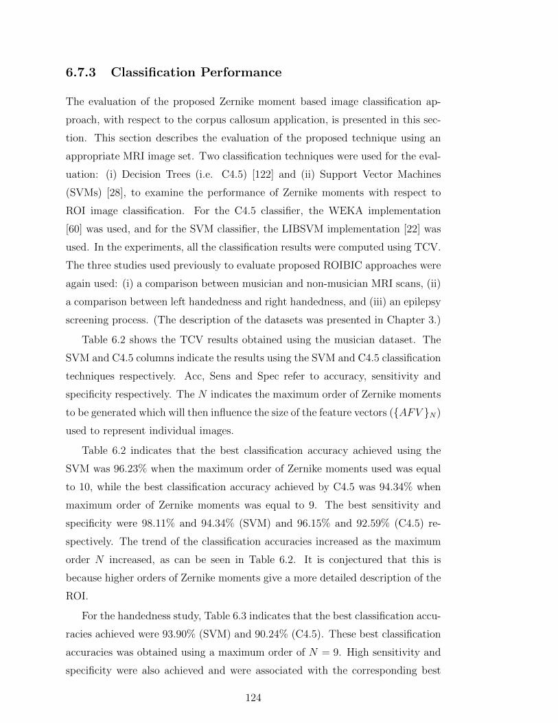
6.7.3 Classification Performance
The evaluation of the proposed Zernike moment based image classification ap-
proach, with respect to the corpus callosum application, is presented in this sec-
tion. This section describes the evaluation of the proposed technique using an
appropriate MRI image set. Two classification techniques were used for the eval-
uation: (i) Decision Trees (i.e. C4.5) [122] and (ii) Support Vector Machines
(SVMs) [28], to examine the performance of Zernike moments with respect to
ROI image classification. For the C4.5 classifier, the WEKA implementation
[60] was used, and for the SVM classifier, the LIBSVM implementation [22] was
used. In the experiments, all the classification results were computed using TCV.
The three studies used previously to evaluate proposed ROIBIC approaches were
again used: (i) a comparison between musician and non-musician MRI scans, (ii)
a comparison between left handedness and right handedness, and (iii) an epilepsy
screening process. (The description of the datasets was presented in Chapter 3.)
Table 6.2 shows the TCV results obtained using the musician dataset. The
SVM and C4.5 columns indicate the results using the SVM and C4.5 classification
techniques respectively. Acc, Sens and Spec refer to accuracy, sensitivity and
specificity respectively. The N indicates the maximum order of Zernike moments
to be generated which will then influence the size of the feature vectors ({AFV }N)
used to represent individual images.
Table 6.2 indicates that the best classification accuracy achieved using the
SVM was 96.23% when the maximum order of Zernike moments used was equal
to 10, while the best classification accuracy achieved by C4.5 was 94.34% when
maximum order of Zernike moments was equal to 9. The best sensitivity and
specificity were 98.11% and 94.34% (SVM) and 96.15% and 92.59% (C4.5) re-
spectively. The trend of the classification accuracies increased as the maximum
order N increased, as can be seen in Table 6.2. It is conjectured that this is
because higher orders of Zernike moments give a more detailed description of the
ROI.
For the handedness study, Table 6.3 indicates that the best classification accu-
racies achieved were 93.90% (SVM) and 90.24% (C4.5). These best classification
accuracies was obtained using a maximum order of N = 9. High sensitivity and
specificity were also achieved and were associated with the corresponding best
124
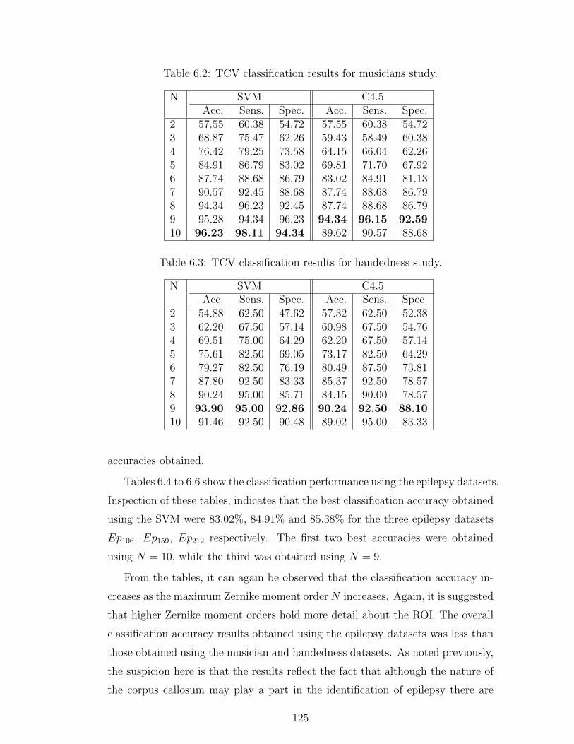
Table 6.2: TCV classification results for musicians study.
N SVM C4.5Acc. Sens. Spec. Acc. Sens. Spec.
2 57.55 60.38 54.72 57.55 60.38 54.723 68.87 75.47 62.26 59.43 58.49 60.384 76.42 79.25 73.58 64.15 66.04 62.265 84.91 86.79 83.02 69.81 71.70 67.926 87.74 88.68 86.79 83.02 84.91 81.137 90.57 92.45 88.68 87.74 88.68 86.798 94.34 96.23 92.45 87.74 88.68 86.799 95.28 94.34 96.23 94.34 96.15 92.5910 96.23 98.11 94.34 89.62 90.57 88.68
Table 6.3: TCV classification results for handedness study.
N SVM C4.5Acc. Sens. Spec. Acc. Sens. Spec.
2 54.88 62.50 47.62 57.32 62.50 52.383 62.20 67.50 57.14 60.98 67.50 54.764 69.51 75.00 64.29 62.20 67.50 57.145 75.61 82.50 69.05 73.17 82.50 64.296 79.27 82.50 76.19 80.49 87.50 73.817 87.80 92.50 83.33 85.37 92.50 78.578 90.24 95.00 85.71 84.15 90.00 78.579 93.90 95.00 92.86 90.24 92.50 88.1010 91.46 92.50 90.48 89.02 95.00 83.33
accuracies obtained.
Tables 6.4 to 6.6 show the classification performance using the epilepsy datasets.
Inspection of these tables, indicates that the best classification accuracy obtained
using the SVM were 83.02%, 84.91% and 85.38% for the three epilepsy datasets
Ep106, Ep159, Ep212 respectively. The first two best accuracies were obtained
using N = 10, while the third was obtained using N = 9.
From the tables, it can again be observed that the classification accuracy in-
creases as the maximum Zernike moment order N increases. Again, it is suggested
that higher Zernike moment orders hold more detail about the ROI. The overall
classification accuracy results obtained using the epilepsy datasets was less than
those obtained using the musician and handedness datasets. As noted previously,
the suspicion here is that the results reflect the fact that although the nature of
the corpus callosum may play a part in the identification of epilepsy there are
125
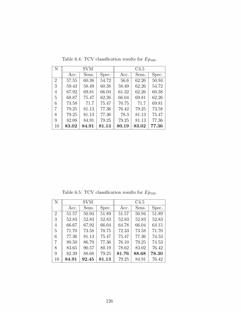
Table 6.4: TCV classification results for Ep106.
N SVM C4.5Acc. Sens. Spec. Acc. Sens. Spec.
2 57.55 60.38 54.72 56.6 62.26 50.943 59.43 58.49 60.38 58.49 62.26 54.724 67.92 69.81 66.04 61.32 62.26 60.385 68.87 75.47 62.26 66.04 69.81 62.266 73.58 71.7 75.47 70.75 71.7 69.817 79.25 81.13 77.36 76.42 79.25 73.588 79.25 81.13 77.36 78.3 81.13 75.479 82.08 84.91 79.25 79.25 81.13 77.3610 83.02 84.91 81.13 80.19 83.02 77.36
Table 6.5: TCV classification results for Ep159.
N SVM C4.5Acc. Sens. Spec. Acc. Sens. Spec.
2 51.57 50.94 51.89 51.57 50.94 51.893 52.83 52.83 52.83 52.83 52.83 52.834 66.67 67.92 66.04 64.78 66.04 64.155 71.70 73.58 70.75 72.33 73.58 71.706 77.36 81.13 75.47 75.47 77.36 74.537 80.50 86.79 77.36 76.10 79.25 74.538 83.65 90.57 80.19 78.62 83.02 76.429 82.39 88.68 79.25 81.76 88.68 78.3010 84.91 92.45 81.13 79.25 84.91 76.42
126
Table 6.6: TCV classification results for Ep212.
N SVM C4.5Acc. Sens. Spec. Acc. Sens. Spec.
2 60.85 64.15 57.55 54.25 55.66 52.833 66.98 70.75 63.21 55.19 56.6 53.774 68.4 74.53 62.26 61.32 65.09 57.555 76.42 81.13 71.7 63.21 67.92 58.496 80.66 85.85 75.47 68.87 75.47 62.267 84.43 86.79 82.08 74.06 78.3 69.818 84.43 86.79 82.08 80.19 84.91 75.479 85.38 87.74 83.02 81.6 86.79 76.4210 84.43 86.79 82.08 80.19 84.91 75.47
also other factors involved.
6.7.4 Time Complexity of the Proposed Classification Ap-proach Based on Zernike Moments
The computation time of the ROI image classification approach based on Zernike
moments, using the three datasets (musician, handedness and Ep212), is pre-
sented in Figure 6.5. All the experiments were performed with 1.86 GHz Intel(R)
Core(TM)2 PC with 2GB RAM. The code was designed using Matlab 7. Note
that the run time complexity increases as the maximum Zernike moments order
increases, this is to be expected as higher values of N necessitate more processing.
6.8 Discussion and Summary
In this chapter a new fast method for computing Zernike moments, based on
a quad-tree decomposition, has been described. A full set of Zernike moments
was used in the context of MR image classification. The use of Zernike moments
is a popular technique in image processing and analysis; this is the reason why
the use of Zernike moments was included in the research described in this thesis.
The reported evaluation indicated that the proposed technique gave reasonable
classification results. The overall performance classification accuracies presented
in Section 6.7 above indicate that:
1. The proposed approach, based on the Zernike moments gives a higher ac-
curacy using high orders of Zernike moments than when using lower orders.
127
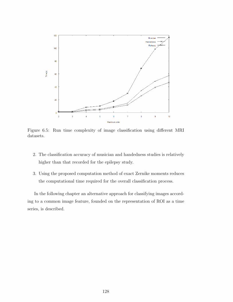
Figure 6.5: Run time complexity of image classification using different MRIdatasets.
2. The classification accuracy of musician and handedness studies is relatively
higher than that recorded for the epilepsy study.
3. Using the proposed computation method of exact Zernike moments reduces
the computational time required for the overall classification process.
In the following chapter an alternative approach for classifying images accord-
ing to a common image feature, founded on the representation of ROI as a time
series, is described.
128
Chapter 7
Region Of Interest ImageClassification Using a TimeSeries Representation
7.1 Introduction
In this chapter, a new approach to ROIBIC, founded on a time series represen-
tation coupled with a Case Based Reasoning (CBR) mechanism, is introduced.
In this approach the features of interest are represented as time series, one per
image. Two techniques for generating the desired time series are considered: (i)
ROI intersection (ROI Int.) time series generation and (ii) radial distance (Rad.
Dist.) time series generation. These time series are then stored in a Case Base
(CB) which can be used to categorise unseen data using a Case Based Reason-
ing (CBR) approach. The unseen data is compared with the categorisations in
the CB using a Dynamic Time Warping (DTW) similarity checking mechanism.
The class associated with the most similar time series (case) in the CB is then
adopted as the class for the unseen data. Note that the phrase “time series”
is used with respect to the adopted representation because the proposed image
classification technique is founded on work on time series analysis, not because
the representation includes some temporal dimension.
The rest of this chapter is organized as follows. Section 7.2 describes the
two techniques for generating the desired ROI time series signature based on the
shape of the ROI. In Section 7.3 the DTW similarity measure used to compare
ROI signatures is presented. The framework for the proposed ROIBIC approach
is presented in Section 7.4, and the evaluation of the proposed approach in Section
129
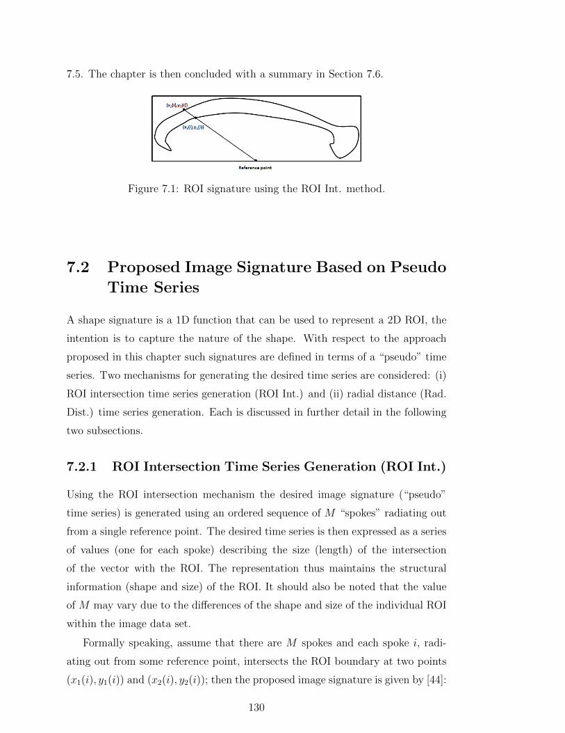
7.5. The chapter is then concluded with a summary in Section 7.6.
Figure 7.1: ROI signature using the ROI Int. method.
7.2 Proposed Image Signature Based on Pseudo
Time Series
A shape signature is a 1D function that can be used to represent a 2D ROI, the
intention is to capture the nature of the shape. With respect to the approach
proposed in this chapter such signatures are defined in terms of a “pseudo” time
series. Two mechanisms for generating the desired time series are considered: (i)
ROI intersection time series generation (ROI Int.) and (ii) radial distance (Rad.
Dist.) time series generation. Each is discussed in further detail in the following
two subsections.
7.2.1 ROI Intersection Time Series Generation (ROI Int.)
Using the ROI intersection mechanism the desired image signature (“pseudo”
time series) is generated using an ordered sequence of M “spokes” radiating out
from a single reference point. The desired time series is then expressed as a series
of values (one for each spoke) describing the size (length) of the intersection
of the vector with the ROI. The representation thus maintains the structural
information (shape and size) of the ROI. It should also be noted that the value
of M may vary due to the differences of the shape and size of the individual ROI
within the image data set.
Formally speaking, assume that there are M spokes and each spoke i, radi-
ating out from some reference point, intersects the ROI boundary at two points
(x1(i), y1(i)) and (x2(i), y2(i)); then the proposed image signature is given by [44]:
130
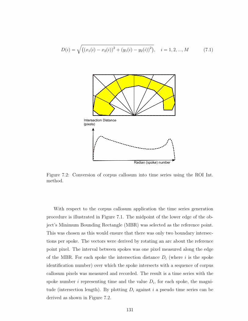
D(i) =√(
(x1(i)− x2(i))2 + (y1(i)− y2(i))2), i = 1, 2, ...,M (7.1)
Figure 7.2: Conversion of corpus callosum into time series using the ROI Int.method.
With respect to the corpus callosum application the time series generation
procedure is illustrated in Figure 7.1. The midpoint of the lower edge of the ob-
ject’s Minimum Bounding Rectangle (MBR) was selected as the reference point.
This was chosen as this would ensure that there was only two boundary intersec-
tions per spoke. The vectors were derived by rotating an arc about the reference
point pixel. The interval between spokes was one pixel measured along the edge
of the MBR. For each spoke the intersection distance Di (where i is the spoke
identification number) over which the spoke intersects with a sequence of corpus
callosum pixels was measured and recorded. The result is a time series with the
spoke number i representing time and the value Di, for each spoke, the magni-
tude (intersection length). By plotting Di against i a pseudo time series can be
derived as shown in Figure 7.2.
131
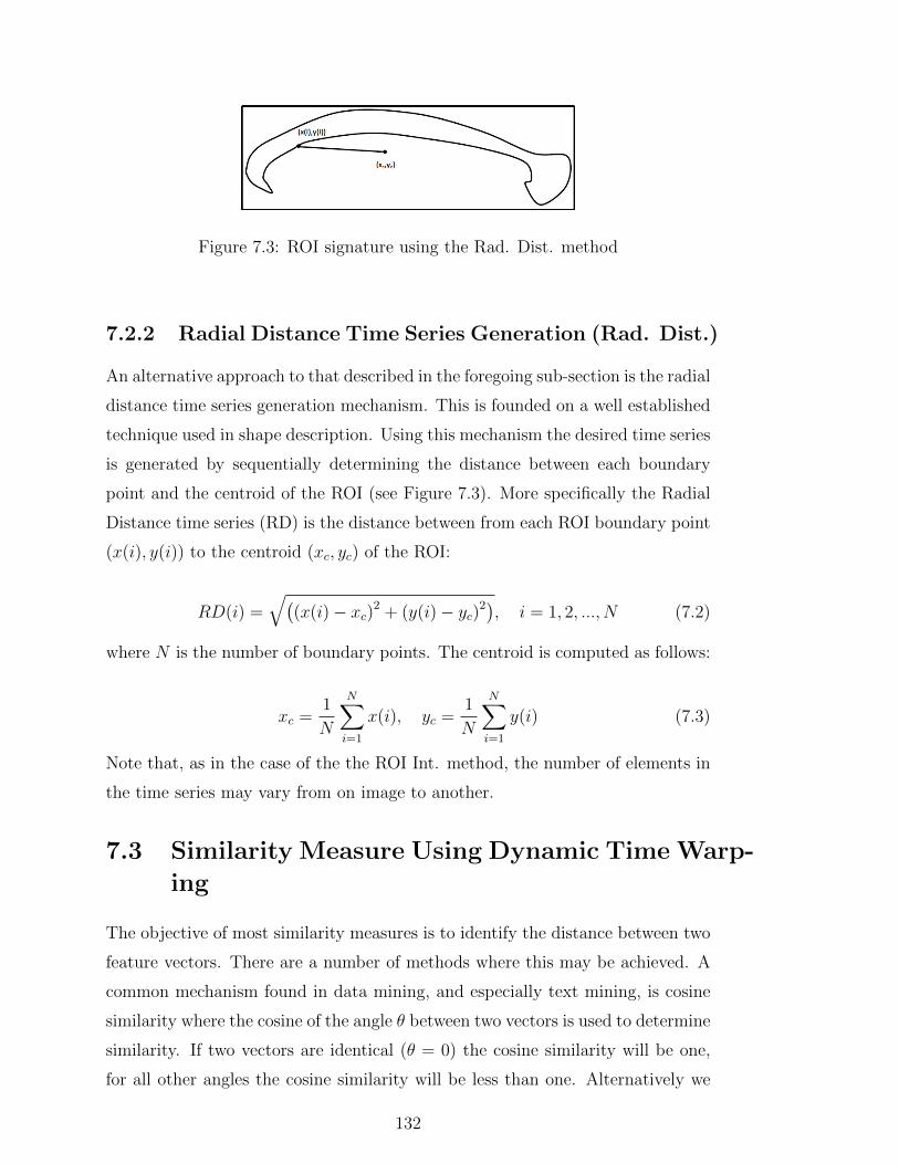
Figure 7.3: ROI signature using the Rad. Dist. method
7.2.2 Radial Distance Time Series Generation (Rad. Dist.)
An alternative approach to that described in the foregoing sub-section is the radial
distance time series generation mechanism. This is founded on a well established
technique used in shape description. Using this mechanism the desired time series
is generated by sequentially determining the distance between each boundary
point and the centroid of the ROI (see Figure 7.3). More specifically the Radial
Distance time series (RD) is the distance between from each ROI boundary point
(x(i), y(i)) to the centroid (xc, yc) of the ROI:
RD(i) =√(
(x(i)− xc)2 + (y(i)− yc)2), i = 1, 2, ..., N (7.2)
where N is the number of boundary points. The centroid is computed as follows:
xc =1
N
N∑i=1
x(i), yc =1
N
N∑i=1
y(i) (7.3)
Note that, as in the case of the the ROI Int. method, the number of elements in
the time series may vary from on image to another.
7.3 Similarity Measure Using Dynamic Time Warp-
ing
The objective of most similarity measures is to identify the distance between two
feature vectors. There are a number of methods where this may be achieved. A
common mechanism found in data mining, and especially text mining, is cosine
similarity where the cosine of the angle θ between two vectors is used to determine
similarity. If two vectors are identical (θ = 0) the cosine similarity will be one,
for all other angles the cosine similarity will be less than one. Alternatively we
132
can compare each element in each vector individually. Both methods require the
vectors to be compared to be identical in length.
In the case of time series the series can also be thought of in terms of feature
vectors, although in this case it would not make sense to adopt measures such
as the cosine measure. However, given two feature vector represented time series
(of identical length), we can compare each pair of corresponding elements in the
two vectors and determine a total difference measure by summing the individual
differences. Various techniques are available to support difference measurement
between feature vector represented time series, for example the Minkowsky met-
ric. However, these techniques are not easily applicable given feature vectors of
different lengths where there is no straight forward one-to-one correspondence
between elements.
The time series used to describe the corpus callosum, as noted in Section
7.2, are not all of the same length; the number of spokes used to generate the
time series is dependent on the size of the MBR surrounding the ROI and the
number of radial distance measurements is dependent on the number of ROI
boundary pixels . In this case an appropriate correspondence may be found
by optimizing over all possible correspondences [130]. One such technique is
Dynamic Time Warping (DTW). The DTW algorithm is a well-known algorithm
in many areas. It was first introduced in 1960s [16] and extensively explored
in 1970s for application within speech recognition systems. It is currently used
in areas such as handwriting recognition and online signature matching [42], and
protein sequence alignment [144]. DTW was adopted with respect to the proposed
approach to allow for the comparison of pairs of corpora callosa.
DTW operates as follows. In order to align two time series (sequences) A
and B with lengths N and M , an N ×M matrix (D) is constructed, where each
element (i, j) of the matrix contains the distance between the points Ai and Bj.
The goal is to find a path through this matrix, which minimizes the sum of the
local distances of the points. An illustration of the alignment between two time
series is shown in Figure 7.4. The path from (1, 1) to (N,M) in the matrix D is
called the warping path W :
W = {w1, w2, ..., wk} (7.4)
133
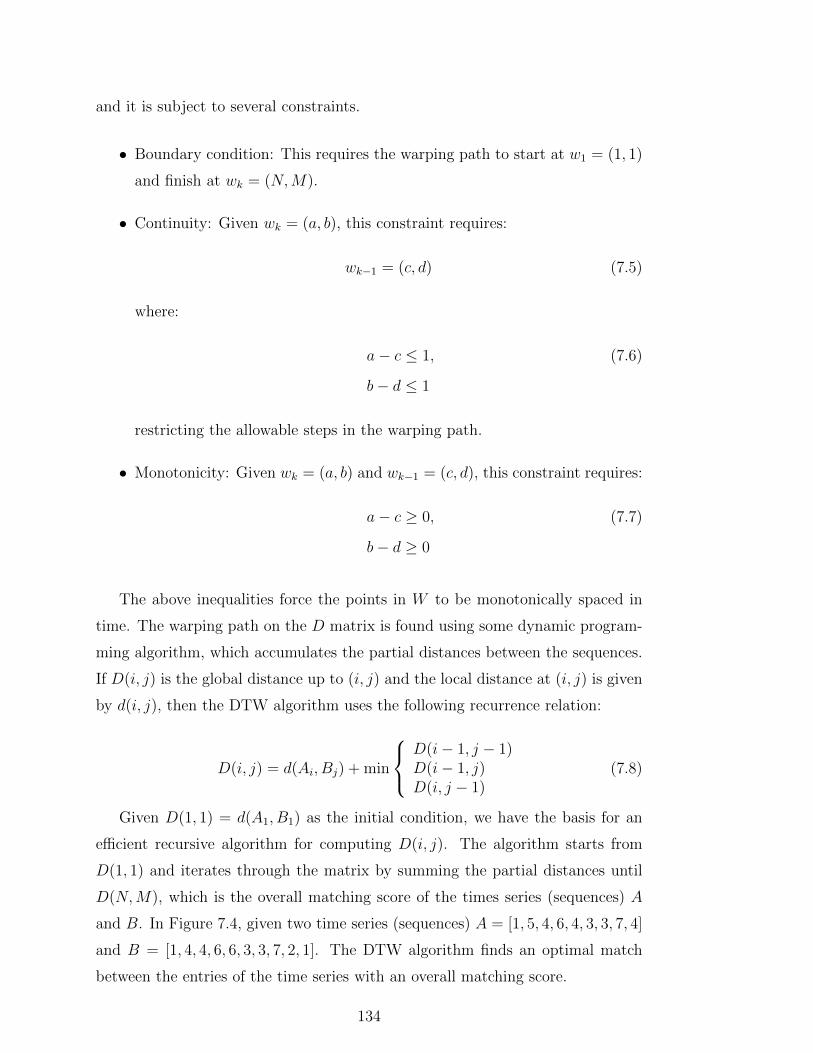
and it is subject to several constraints.
• Boundary condition: This requires the warping path to start at w1 = (1, 1)
and finish at wk = (N,M).
• Continuity: Given wk = (a, b), this constraint requires:
wk−1 = (c, d) (7.5)
where:
a− c ≤ 1, (7.6)
b− d ≤ 1
restricting the allowable steps in the warping path.
• Monotonicity: Given wk = (a, b) and wk−1 = (c, d), this constraint requires:
a− c ≥ 0, (7.7)
b− d ≥ 0
The above inequalities force the points in W to be monotonically spaced in
time. The warping path on the D matrix is found using some dynamic program-
ming algorithm, which accumulates the partial distances between the sequences.
If D(i, j) is the global distance up to (i, j) and the local distance at (i, j) is given
by d(i, j), then the DTW algorithm uses the following recurrence relation:
D(i, j) = d(Ai, Bj) + min
D(i− 1, j − 1)D(i− 1, j)D(i, j − 1)
(7.8)
Given D(1, 1) = d(A1, B1) as the initial condition, we have the basis for an
efficient recursive algorithm for computing D(i, j). The algorithm starts from
D(1, 1) and iterates through the matrix by summing the partial distances until
D(N,M), which is the overall matching score of the times series (sequences) A
and B. In Figure 7.4, given two time series (sequences) A = [1, 5, 4, 6, 4, 3, 3, 7, 4]
and B = [1, 4, 4, 6, 6, 3, 3, 7, 2, 1]. The DTW algorithm finds an optimal match
between the entries of the time series with an overall matching score.
134
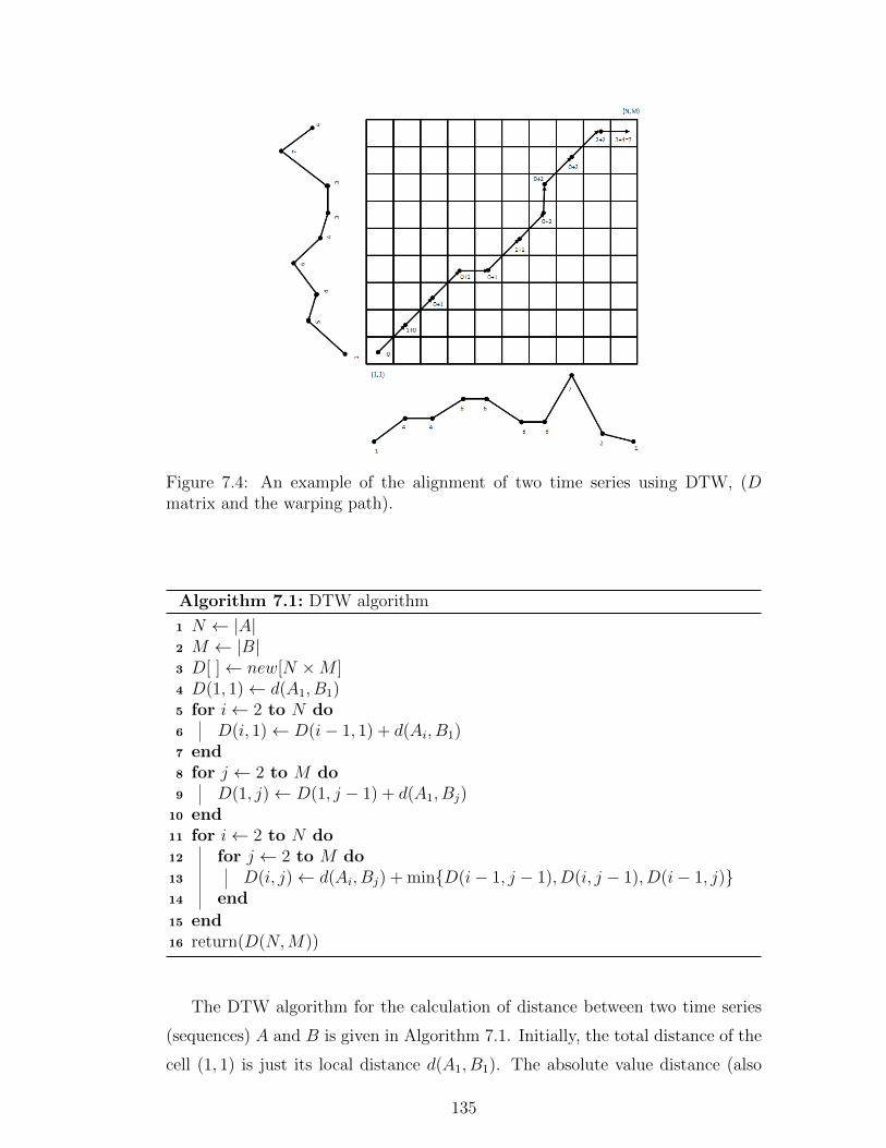
Figure 7.4: An example of the alignment of two time series using DTW, (Dmatrix and the warping path).
Algorithm 7.1: DTW algorithm
1 N ← |A|2 M ← |B|3 D[ ]← new[N ×M ]4 D(1, 1)← d(A1, B1)5 for i← 2 to N do6 D(i, 1)← D(i− 1, 1) + d(Ai, B1)7 end8 for j ← 2 to M do9 D(1, j)← D(1, j − 1) + d(A1, Bj)
10 end11 for i← 2 to N do12 for j ← 2 to M do13 D(i, j)← d(Ai, Bj) + min{D(i− 1, j − 1), D(i, j − 1), D(i− 1, j)}14 end
15 end16 return(D(N,M))
The DTW algorithm for the calculation of distance between two time series
(sequences) A and B is given in Algorithm 7.1. Initially, the total distance of the
cell (1, 1) is just its local distance d(A1, B1). The absolute value distance (also
135
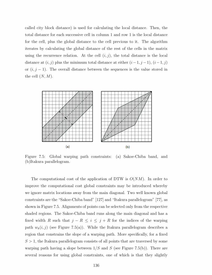
called city block distance) is used for calculating the local distance. Then, the
total distance for each successive cell in column 1 and row 1 is the local distance
for the cell, plus the global distance to the cell previous to it. The algorithm
iterates by calculating the global distance of the rest of the cells in the matrix
using the recurrence relation. At the cell (i, j), the total distance is the local
distance at (i, j) plus the minimum total distance at either (i−1, j−1), (i−1, j)
or (i, j − 1). The overall distance between the sequences is the value stored in
the cell (N,M).
Figure 7.5: Global warping path constraints: (a) Sakoe-Chiba band, and(b)Itakura parallelogram.
The computational cost of the application of DTW is O(NM). In order to
improve the computational cost global constraints may be introduced whereby
we ignore matrix locations away from the main diagonal. Two well known global
constraints are the “Sakoe-Chiba band” [127] and “Itakura parallelogram” [77], as
shown in Figure 7.5. Alignments of points can be selected only from the respective
shaded regions. The Sakoe-Chiba band runs along the main diagonal and has a
fixed width R such that j − R ≤ i ≤ j + R for the indices of the warping
path wk(i, j) (see Figure 7.5(a)). While the Itakura parallelogram describes a
region that constrains the slope of a warping path. More specifically, for a fixed
S > 1, the Itakura parallelogram consists of all points that are traversed by some
warping path having a slope between 1/S and S (see Figure 7.5(b)). There are
several reasons for using global constraints, one of which is that they slightly
136
speed up the DTW distance calculation. However, the most important reason
is to prevent pathological warpings, where a relatively small section of one time
series maps onto a relatively large section of another. In the work described here,
the Sakoe-Chiba band was adopted.
7.4 Framework for Image Classification Based
on Time Series Representation
The time series based image classification approach commences with the segmen-
tation and registration of the input images as described in Chapter 3. Once the
ROI have been segmented and identified the next step is to derive the time series
according to the boundary line circumscribing the ROI. In each case the ROI is
then represented using the proposed time series generation techniques described
in Section 7.2. Each ROI signature is then conceptualised as a proto-type or
case contained in a Case Base (CB), to which a Case Based Reasoning (CBR)
mechanism can be applied. As noted in Chapter 2, CBR is a branch of Artificial
Intelligence (AI) founded on the idea that humans solve problems according to
their experience, i.e. CBR conjectures that humans solve problems by attempting
to match previous successfully addressed problems to the current problem. As
such a CBR system comprises a Case Base (CB) and some matching strategy to
align a new problem (case) with previously solved problems (cases) in the CB.
Typically it will not be possible to find an exact match and thus some matching
strategy will have to be adopted to find the most relevant case or cases.
As noted previously CBR can be used for classification purposes where, given
an unseen record (case), the record can be classified according to the “best match”
discovered in the CB. With respect to proposed technique, and in the case of the
corpus callosum application, the CB comprises a set of pre-labelled (classified)
ROI time series “signatures”, each describing a ROI record. The DTW time
series matching strategy was then adopted to identify a best match with a new
(“unseen”) ROI signature. To do this each pre-labelled (classified) signature of
size N was compared to the test signature of size M using the DTW technique
and a sequence of similarity measures obtained. The well established k-nearest
neighbour technique (KNN) was used to identify the most similar signature in the
CB from which a class label was then extracted. In the experiments reported in
137
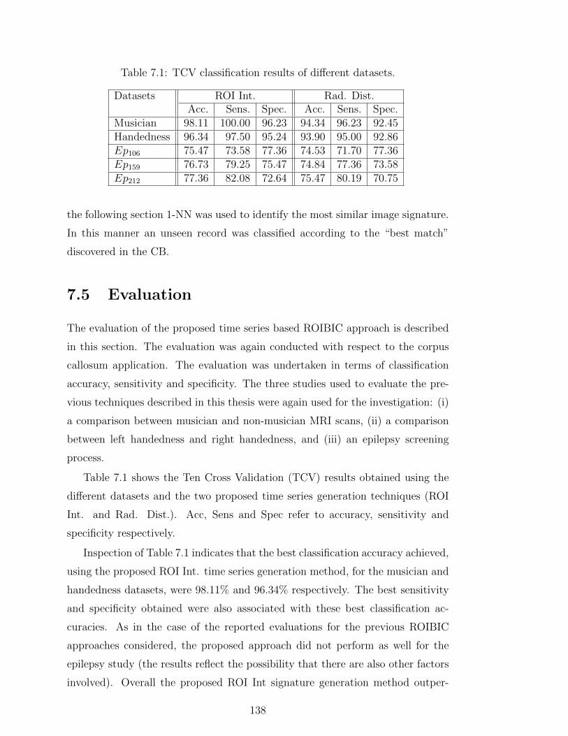
Table 7.1: TCV classification results of different datasets.
Datasets ROI Int. Rad. Dist.Acc. Sens. Spec. Acc. Sens. Spec.
Musician 98.11 100.00 96.23 94.34 96.23 92.45Handedness 96.34 97.50 95.24 93.90 95.00 92.86Ep106 75.47 73.58 77.36 74.53 71.70 77.36Ep159 76.73 79.25 75.47 74.84 77.36 73.58Ep212 77.36 82.08 72.64 75.47 80.19 70.75
the following section 1-NN was used to identify the most similar image signature.
In this manner an unseen record was classified according to the “best match”
discovered in the CB.
7.5 Evaluation
The evaluation of the proposed time series based ROIBIC approach is described
in this section. The evaluation was again conducted with respect to the corpus
callosum application. The evaluation was undertaken in terms of classification
accuracy, sensitivity and specificity. The three studies used to evaluate the pre-
vious techniques described in this thesis were again used for the investigation: (i)
a comparison between musician and non-musician MRI scans, (ii) a comparison
between left handedness and right handedness, and (iii) an epilepsy screening
process.
Table 7.1 shows the Ten Cross Validation (TCV) results obtained using the
different datasets and the two proposed time series generation techniques (ROI
Int. and Rad. Dist.). Acc, Sens and Spec refer to accuracy, sensitivity and
specificity respectively.
Inspection of Table 7.1 indicates that the best classification accuracy achieved,
using the proposed ROI Int. time series generation method, for the musician and
handedness datasets, were 98.11% and 96.34% respectively. The best sensitivity
and specificity obtained were also associated with these best classification ac-
curacies. As in the case of the reported evaluations for the previous ROIBIC
approaches considered, the proposed approach did not perform as well for the
epilepsy study (the results reflect the possibility that there are also other factors
involved). Overall the proposed ROI Int signature generation method outper-
138
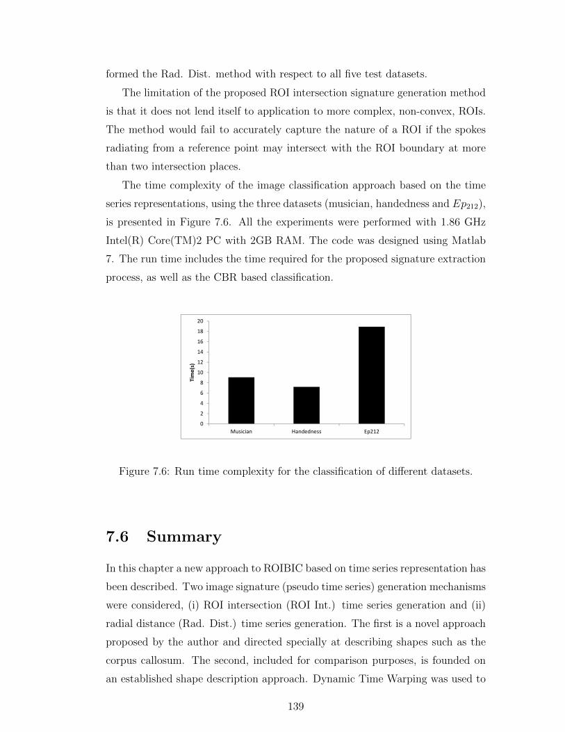
formed the Rad. Dist. method with respect to all five test datasets.
The limitation of the proposed ROI intersection signature generation method
is that it does not lend itself to application to more complex, non-convex, ROIs.
The method would fail to accurately capture the nature of a ROI if the spokes
radiating from a reference point may intersect with the ROI boundary at more
than two intersection places.
The time complexity of the image classification approach based on the time
series representations, using the three datasets (musician, handedness and Ep212),
is presented in Figure 7.6. All the experiments were performed with 1.86 GHz
Intel(R) Core(TM)2 PC with 2GB RAM. The code was designed using Matlab
7. The run time includes the time required for the proposed signature extraction
process, as well as the CBR based classification.
0
2
4
6
8
10
12
14
16
18
20
Musician Handedness Ep212
Tim
e(s)
Figure 7.6: Run time complexity for the classification of different datasets.
7.6 Summary
In this chapter a new approach to ROIBIC based on time series representation has
been described. Two image signature (pseudo time series) generation mechanisms
were considered, (i) ROI intersection (ROI Int.) time series generation and (ii)
radial distance (Rad. Dist.) time series generation. The first is a novel approach
proposed by the author and directed specially at describing shapes such as the
corpus callosum. The second, included for comparison purposes, is founded on
an established shape description approach. Dynamic Time Warping was used to
139

compare signatures as part of a CBR framework used to classify new records. The
reported evaluation indicated that the ROI Int. time series generation method
gave the best performance.
140
Chapter 8
Conclusion
A summary of the proposed ROI image classification approaches, the compari-
son between these approaches, the main findings, the research contribution and
possible future directions, are presented in this chapter. Section 8.1 gives the
summary of the proposed ROI image classification approaches. The comparison
between these approaches with respect to their performance on the test data sets
is presented in Section 8.2. Statistical comparison between theses approaches is
presented in Section 8.3. The main findings and the contribution of the research
work are presented in Section 8.4. Finally some directions for future research are
presented in Section 8.5.
8.1 Summary
Four different ROIBIC approaches were proposed in this thesis to classifying
(categorise) MRI brain scans according to the nature of the corpus callosum, a
structure within the mammalian brain that connects the two brain hemispheres.
The evaluation of these four approaches, on different data sets derived from the
medical domain, suggests that there is no single ROIBIC approach that is best
suited to all the image data sets considered. All the four ROIBIC approaches
commenced with an image segmentation process so as to isolate and extract
the desired ROI (the corpus callosum with respect to the scenario that formed
the focus for the work described in this thesis). A variation of the Multiscale
Normalized Cuts algorithm was proposed to achieve the desired segmentation. All
the four ROI image classification approaches, although operating in very different
manners, are essentially supervised learning mechanisms whereby a prelabelled
141
training set was used to build a “classifier” which can then be applied to unseen
data.
The first approach was founded on the concept of the Hough transform coupled
with a polygonal approximation. The aim of the application of the polygonal
approximation to the ROI was to obtain a smooth curve over a minimum number
of line segments describing the regions boundary. The Hough transform was
then used to extract a (1D) image signature vector, one per each image. The
signatures from a labelled training set can thus be collected together and stored
in a Case Base (CB) within a Case Based Reasoning (CBR) framework to be used
in the context of image classification. The reported evaluation indicated that the
proposed technique performed well in the case of the application of polygonal
approximation compared with not using such an approximation.
The second approach was founded on the concept of graph mining. This ap-
proach used a hierarchical decomposition technique, coupled with a quad-tree
based representation, one tree per image. A weighted frequent subgraph mining
algorithm, gSpan-ATW, was then applied to identify frequently occurring sub-
graphs (subtrees) within the quad-tree representation. The general assumption
for the application of the algorithm was that quad-tree nodes further away from
the root were more significant than those nearer the root because the more distant
nodes encapsulated a greater level of detail. The identified frequent subtrees were
viewed as defining a feature space which could be used to represent the image
set. A given image set can thus be recast into this format so that each image is
represented by a feature vector whose elements are some subset of the global set
of identified frequent subtrees making up the feature space. Standard classifier
generation techniques can then be applied to build a classifier that can be ap-
plied to unseen data. The reported evaluation indicated that high classification
accuracy results were obtained when using higher quad-tree decomposition levels
coupled with low support thresholds.
The third approach was founded on using Zernike moments. A new method
for the fast computation of Zernike moments, also based on a quad-tree decompo-
sition, was proposed. Using the proposed computation method for the generation
of exact Zernike moments reduced the computational time required for the overall
classification process. A full set of Zernike moments was used in the context of
142
the desired MR image classification. The reported evaluation indicated that the
proposed technique gave more reasonable classification results using high orders
of Zernike moments than when using lower orders.
The fourth approach was founded on the representation of ROI as time series.
A new image signature generation mechanism, based on the size and shape of the
ROI, was proposed. As in the case of the proposed Hough transform technique,
the time series representing a particular image set were collected together in a
CB forming part of a CBR framework. A dynamic time warping technique was
adopted to calculate the similarity between new cases and time series held in
the CB. The reported evaluation revealed that the proposed technique performed
well with respect to the musicians and handedness studies, but not so well with
respect to the epilepsy study.
8.2 Comparison of the Proposed Approaches
The four advocated approaches to ROI based image classification were evaluated
in the context of the classification of brain MRI scans according to the nature of
a particular ROI that appears across such datasets, namely the corpus callosum.
This sections reports on an overall comparison between these approaches. The
comparison was undertaken in terms of classification performance and run time
complexity. The evaluation of each approach reported in the foregoing chapters,
considered the effect of parameter settings associated with each approach, and
is some cases variations of the approach. For the overall comparison reported
in this section the best performing parameters and/or variations with respect to
each technique were used (so as to consider each technique to its best advan-
tage). Moreover, the proposed approaches were compared with the two notable
techniques: the Curvature Scale Space (CSS) [102] (see Section 2.5.2.7) and the
Angular Radial Transform (ART) [19] (see Section 2.5.1.3). These two techniques
were used in this comparison because in the MPEG-7 standard, the curvature
scale space (CSS) has been adopted as the contour-based shape descriptor and
the angular radial transform (ART) has been adopted as the region-based shape
descriptor.
Table 8.1 shows the TCV results obtained using the musician data set. The
HT, GB, ZM, TS rows indicate the results using the Hough Transform, graph,
143
Zernike moments, and time series based approaches respectively. The CSS, ART
rows indicate the MPEG-7 descriptors (Curvature Scale Space and the Angular
Radial Transform) respectively. The Acc, Sens, and Spec columns indicate ac-
curacy, sensitivity and specificity respectively. The best results are indicated in
bold font. Inspection of Table 8.1 demonstrates that the overall classification
accuracies obtained using the four advocated approaches were over 90%, while
the overall classification accuracy obtained using the time series based approach
significantly improved over that obtained using the other three approaches. The
best sensitivity and specificity were also obtained using the time series based
approach. The four advocated approaches also outperform the CSS and ART
techniques. These are excellent results.
Table 8.2 shows the TCV results obtained using the handedness data set.
The column and row headers are defined as in Table 8.1. Inspection of Table 8.2
indicates that the four advocated approaches also performed well with respect
to handedness study. The best overall classification results were again obtained
using the time series based approach, which showed significant improvement over
the other three approaches. The best sensitivity and specificity were also ob-
tained also using time series based approach. The four advocated approaches
also outperform the CSS and ART techniques. Again, these are excellent results.
Table 8.3 shows the TCV results obtained using the epilepsy data set (Ep212).
The column and row headers were defined as in Table 8.1. Inspection of Table
8.3 demonstrates that the Hough transform and time series based approaches
did not perform as well as the other two approaches. The graph based and
Zernike moments based approaches that consider all the pixels of each ROI in
the feature extraction process outperformed the Hough transform and time series
based approaches (recall that these approaches consider only the pixels of the
boundary of the ROI). The four advocated approaches also outperform the CSS
and ART techniques. The results for the epilepsy data set seem to be at odds
with those obtained using the musicians and handedness studies. This was also
noted with respect to the individual evaluations reported earlier in this thesis.
Subsequent discussion with medical domain experts did not give an indication as
to why this might be the case. However, as noted earlier, the suspicion is that
the results reflect the fact that although the nature of the corpus callosum may
144
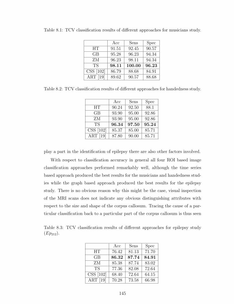
Table 8.1: TCV classification results of different approaches for musicians study.
Acc Sens SpecHT 91.51 92.45 90.57GB 95.28 96.23 94.34ZM 96.23 98.11 94.34TS 98.11 100.00 96.23
CSS [102] 86.79 88.68 84.91ART [19] 89.62 90.57 88.68
Table 8.2: TCV classification results of different approaches for handedness study.
Acc Sens SpecHT 90.24 92.50 88.1GB 93.90 95.00 92.86ZM 93.90 95.00 92.86TS 96.34 97.50 95.24
CSS [102] 85.37 85.00 85.71ART [19] 87.80 90.00 85.71
play a part in the identification of epilepsy there are also other factors involved.
With respect to classification accuracy in general all four ROI based image
classification approaches performed remarkably well, although the time series
based approach produced the best results for the musicians and handedness stud-
ies while the graph based approach produced the best results for the epilepsy
study. There is no obvious reason why this might be the case, visual inspection
of the MRI scans does not indicate any obvious distinguishing attributes with
respect to the size and shape of the corpus callosum. Tracing the cause of a par-
ticular classification back to a particular part of the corpus callosum is thus seen
Table 8.3: TCV classification results of different approaches for epilepsy study(Ep212).
Acc Sens SpecHT 76.42 81.13 71.70GB 86.32 87.74 84.91ZM 85.38 87.74 83.02TS 77.36 82.08 72.64
CSS [102] 68.40 72.64 64.15ART [19] 70.28 73.58 66.98
145
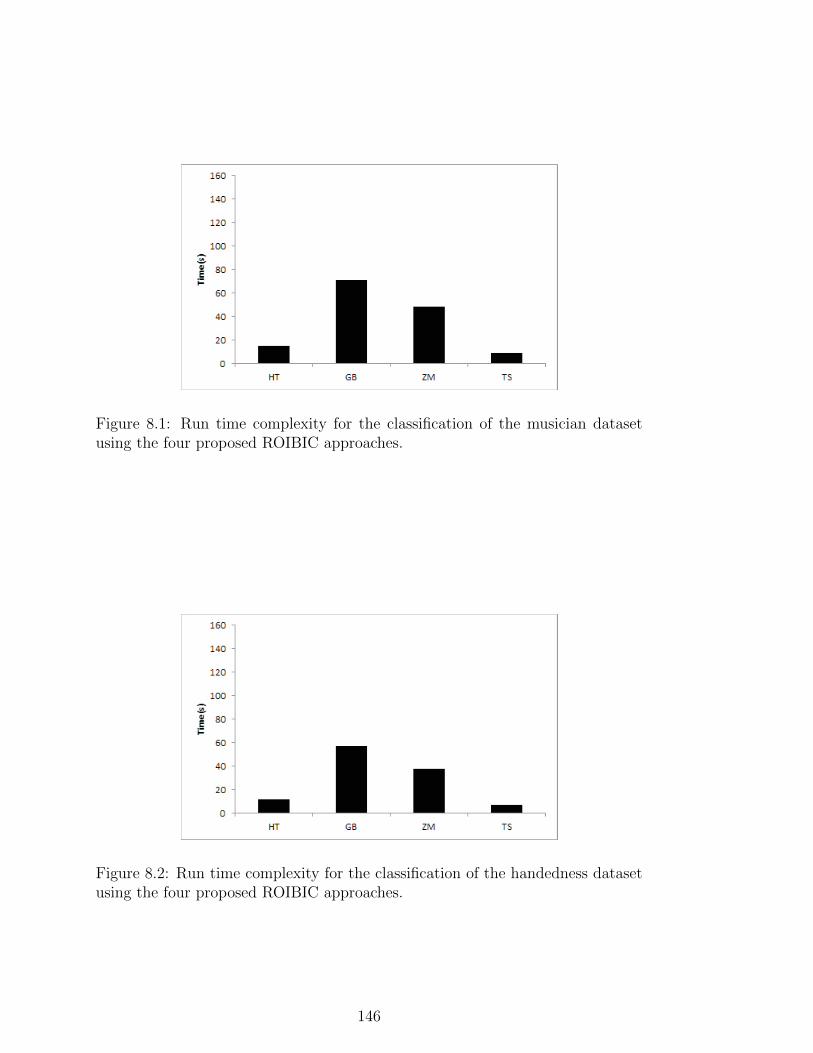
Figure 8.1: Run time complexity for the classification of the musician datasetusing the four proposed ROIBIC approaches.
Figure 8.2: Run time complexity for the classification of the handedness datasetusing the four proposed ROIBIC approaches.
146
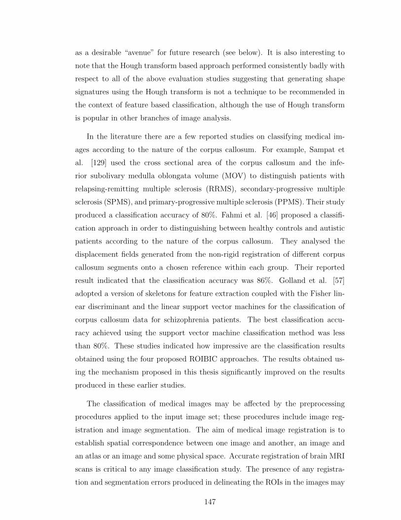
as a desirable “avenue” for future research (see below). It is also interesting to
note that the Hough transform based approach performed consistently badly with
respect to all of the above evaluation studies suggesting that generating shape
signatures using the Hough transform is not a technique to be recommended in
the context of feature based classification, although the use of Hough transform
is popular in other branches of image analysis.
In the literature there are a few reported studies on classifying medical im-
ages according to the nature of the corpus callosum. For example, Sampat et
al. [129] used the cross sectional area of the corpus callosum and the infe-
rior subolivary medulla oblongata volume (MOV) to distinguish patients with
relapsing-remitting multiple sclerosis (RRMS), secondary-progressive multiple
sclerosis (SPMS), and primary-progressive multiple sclerosis (PPMS). Their study
produced a classification accuracy of 80%. Fahmi et al. [46] proposed a classifi-
cation approach in order to distinguishing between healthy controls and autistic
patients according to the nature of the corpus callosum. They analysed the
displacement fields generated from the non-rigid registration of different corpus
callosum segments onto a chosen reference within each group. Their reported
result indicated that the classification accuracy was 86%. Golland et al. [57]
adopted a version of skeletons for feature extraction coupled with the Fisher lin-
ear discriminant and the linear support vector machines for the classification of
corpus callosum data for schizophrenia patients. The best classification accu-
racy achieved using the support vector machine classification method was less
than 80%. These studies indicated how impressive are the classification results
obtained using the four proposed ROIBIC approaches. The results obtained us-
ing the mechanism proposed in this thesis significantly improved on the results
produced in these earlier studies.
The classification of medical images may be affected by the preprocessing
procedures applied to the input image set; these procedures include image reg-
istration and image segmentation. The aim of medical image registration is to
establish spatial correspondence between one image and another, an image and
an atlas or an image and some physical space. Accurate registration of brain MRI
scans is critical to any image classification study. The presence of any registra-
tion and segmentation errors produced in delineating the ROIs in the images may
147
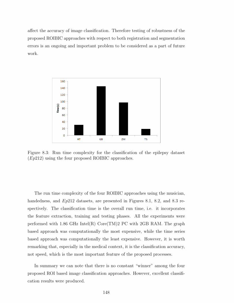
affect the accuracy of image classification. Therefore testing of robustness of the
proposed ROIBIC approaches with respect to both registration and segmentation
errors is an ongoing and important problem to be considered as a part of future
work.
Figure 8.3: Run time complexity for the classification of the epilepsy dataset(Ep212) using the four proposed ROIBIC approaches.
The run time complexity of the four ROIBIC approaches using the musician,
handedness, and Ep212 datasets, are presented in Figures 8.1, 8.2, and 8.3 re-
spectively. The classification time is the overall run time, i.e. it incorporates
the feature extraction, training and testing phases. All the experiments were
performed with 1.86 GHz Intel(R) Core(TM)2 PC with 2GB RAM. The graph
based approach was computationally the most expensive, while the time series
based approach was computationally the least expensive. However, it is worth
remarking that, especially in the medical context, it is the classification accuracy,
not speed, which is the most important feature of the proposed processes.
In summary we can note that there is no constant “winner” among the four
proposed ROI based image classification approaches. However, excellent classifi-
cation results were produced.
148
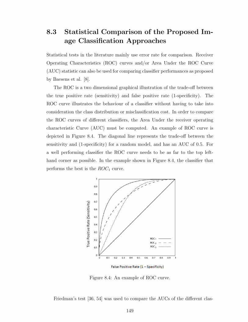
8.3 Statistical Comparison of the Proposed Im-
age Classification Approaches
Statistical tests in the literature mainly use error rate for comparison. Receiver
Operating Characteristics (ROC) curves and/or Area Under the ROC Curve
(AUC) statistic can also be used for comparing classifier performances as proposed
by Baesens et al. [8].
The ROC is a two dimensional graphical illustration of the trade-off between
the true positive rate (sensitivity) and false positive rate (1-specificity). The
ROC curve illustrates the behaviour of a classifier without having to take into
consideration the class distribution or misclassification cost. In order to compare
the ROC curves of different classifiers, the Area Under the receiver operating
characteristic Curve (AUC) must be computed. An example of ROC curve is
depicted in Figure 8.4. The diagonal line represents the trade-off between the
sensitivity and (1-specificity) for a random model, and has an AUC of 0.5. For
a well performing classifier the ROC curve needs to be as far to the top left-
hand corner as possible. In the example shown in Figure 8.4, the classifier that
performs the best is the ROC1 curve.
Figure 8.4: An example of ROC curve.
Friedman’s test [36, 54] was used to compare the AUCs of the different clas-
149
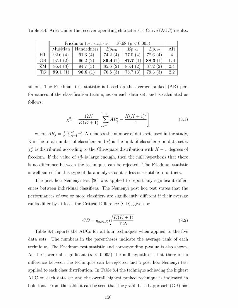
Table 8.4: Area Under the receiver operating characteristic Curve (AUC) results.
Friedman test statistic = 10.68 (p < 0.005)Musician Handedness Ep106 Ep159 Ep212 AR
HT 92.6 (4) 91.3 (4) 74.2 (4) 77.0 (4) 78.6 (4) 4GB 97.1 (2) 96.2 (2) 86.4 (1) 87.7 (1) 88.3 (1) 1.4ZM 96.4 (3) 94.7 (3) 85.6 (2) 86.4 (2) 87.2 (2) 2.4TS 99.1 (1) 96.8 (1) 76.5 (3) 78.7 (3) 79.3 (3) 2.2
sifiers. The Friedman test statistic is based on the average ranked (AR) per-
formances of the classification techniques on each data set, and is calculated as
follows:
χ2F =
12N
K(K + 1)
[K∑j=1
AR2j −
K(K + 1)2
4
](8.1)
where ARj = 1N
∑Ni=1 r
ji , N denotes the number of data sets used in the study,
K is the total number of classifiers and rji is the rank of classifier j on data set i.
χ2F is distributed according to the Chi-square distribution with K − 1 degrees of
freedom. If the value of χ2F is large enough, then the null hypothesis that there
is no difference between the techniques can be rejected. The Friedman statistic
is well suited for this type of data analysis as it is less susceptible to outliers.
The post hoc Nemenyi test [36] was applied to report any significant differ-
ences between individual classifiers. The Nemenyi post hoc test states that the
performances of two or more classifiers are significantly different if their average
ranks differ by at least the Critical Difference (CD), given by
CD = qα,∞,K
√K(K + 1)
12N(8.2)
Table 8.4 reports the AUCs for all four techniques when applied to the five
data sets. The numbers in the parentheses indicate the average rank of each
technique. The Friedman test statistic and corresponding p-value is also shown.
As these were all significant (p < 0.005) the null hypothesis that there is no
difference between the techniques can be rejected and a post hoc Nemenyi test
applied to each class distribution. In Table 8.4 the technique achieving the highest
AUC on each data set and the overall highest ranked technique is indicated in
bold font. From the table it can be seen that the graph based approach (GB) has
150
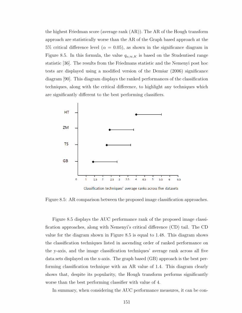
the highest Friedman score (average rank (AR)). The AR of the Hough transform
approach are statistically worse than the AR of the Graph based approach at the
5% critical difference level (α = 0.05), as shown in the significance diagram in
Figure 8.5. In this formula, the value qα,∞,K is based on the Studentised range
statistic [36]. The results from the Friedmans statistic and the Nemenyi post hoc
tests are displayed using a modified version of the Demsar (2006) significance
diagram [90]. This diagram displays the ranked performances of the classification
techniques, along with the critical difference, to highlight any techniques which
are significantly different to the best performing classifiers.
Figure 8.5: AR comparison between the proposed image classification approaches.
Figure 8.5 displays the AUC performance rank of the proposed image classi-
fication approaches, along with Nemenyi’s critical difference (CD) tail. The CD
value for the diagram shown in Figure 8.5 is equal to 1.48. This diagram shows
the classification techniques listed in ascending order of ranked performance on
the y-axis, and the image classification techniques’ average rank across all five
data sets displayed on the x-axis. The graph based (GB) approach is the best per-
forming classification technique with an AR value of 1.4. This diagram clearly
shows that, despite its popularity, the Hough transform performs significantly
worse than the best performing classifier with value of 4.
In summary, when considering the AUC performance measures, it can be con-
151
cluded that the graph based technique yields a very good performance. However,
Hough transform approach performs significantly worse than the best performing
technique. The majority of classification techniques yielded classification perfor-
mances that are quite competitive with each other.
8.4 Main Findings and Contributions
In this thesis, the concept of image classification according to the nature of ROIs
contained within image data set, was considered. Four ROIBIC approaches were
proposed. These approaches considered four different ROI representations to
maintain the structural information (shape and size) of ROIs coupled with an
appropriate classification technique. The proposed approaches were designed to
address the research question introduced in Chapter 1 and a number of associated
research issues. In this Section the research question and issues are returned to.
In the following each of the identified research issues is discussed in turn and the
manner in which the proposed research addresses each individual issue briefly
highlighted.
(a) “The techniques derived should serve to maximize classification
accuracy.”
The proposed approaches, as described in Chapters 4, 5, 6 and 7, were able
to achieve high classification accuracy in the context of classifying different
image data sets.
(b) “To achieve the desired classification accuracy any proposed fea-
ture extraction (representation) method should capture the salient
elements of the ROI without knowing in advance what those salient
elements might be. In other words any proposed feature extrac-
tion method, whatever form this might take, should retain as much
relevant information as possible.”
According to the work described in Chapters 4, 5, 6 and 7, the different
representations of ROI were able to capture the salient elements of the ROI
under consideration (the corpus callosum) so as to maintain the structural
information (shape and size) of these ROIs. As proposed in Chapter 5, the
152
application of a weighting scheme puts an emphasis on the most important
frequent subgraphs instead of identifying all the frequent subgraphs during
the mining process. Also, using exact Zernike moments with a higher order,
effectively captures the salient elements of a ROI as described in Chapter 6.
Similarly, the signature approach based on the Hough transform and the time
series approaches were also able to capture these salient elements.
(c) “It is also desirable to conduct the classification in reasonable time,
there is thus a trade off between accuracy and efficiency that must
be addressed.”
Some of the proposed approaches conducted the desired classification in rea-
sonable time, such as the Hough transform and time series approaches (with-
out any speed up mechanisms). With regard to the graph based approach,
the application of a weighting scheme (ATW) enabled the weighted FSM al-
gorithm (gSpan-ATW) to identify a significantly smaller number of frequent
subgraphs than might have been achieved using standard FSM algorithms.
Of note also is the mechanism proposed to speed up of the computation of
exact Zernike moments so as to reduce the overall classification time with
respect to the Zernike moments approach.
(d) “Not all potential representations are compatible with all available
classification paradigms, thus different representations may require
the application of different classification techniques.”
The proposed approaches worked in different manners according to the nature
of the proposed ROI representation. Using the Hough transform and time
series approaches a CBR technique was adopted to classify the unseen cases.
Although different similarity measures were used, euclidean distance for the
Hough transform technique and DTW for the time series based approach.
Standard classification techniques (SVM and decision trees) were adopted
in the case of the graph and Zernike moments based approaches. Therefore
it is possible to conclude that the adopted classification mechanism were
dependent on the nature of the ROI representation technique adopted.
Returning to Chapter 1, the overriding research question was: “How best
to process image collections so that efficient and effective classifica-
153
tion, according to some ROI contained across the image set, can be
achieved?”
The work described in the foregoing chapters clearly indicates that the answer
to this question is that the proposed ROI representations, coupled with appro-
priate classification techniques, can clearly classify such images in a way that is
both efficient and effective.
The primary contributions of the research work presented in this thesis can
thus be summarized as follows:
(a) A variation of the multiscale normalized cuts algorithm to achieve the desired
segmentation and delineating of a ROI contained across an image data set.
(b) A novel approach to MR image classification based on the Hough transform
coupled with a polygonal approximation.
(c) An effective approach to MR image classification based on a quad tree repre-
sented hierarchical decomposition coupled with a weighted frequent subgraph
mining algorithm.
(d) A novel mechanism to speed up the computation of exact Zernike Moments,
also based on a quad-tree decomposition, and the usage of the resulting
Zernike moments to define signatures for input to a classification system.
(e) An effective mechanism to describe ROIs in the form of a time series cou-
pled with the use dynamic time warping to determine the similarity between
images within the context of a CBR framework.
8.5 Future Work
The research described in this thesis has sparked a number of promising directions
for future research. In the concluding section of this chapter, and this thesis, these
future research directions are briefly outlined below.
• Explanation facility. In Section 8.2 it was noted that although excellent
classification results were produced (using all four methods) none of the
methods included an explanation facility. If any of the proposed techniques
are to be used in clinical practice the clinicians using the techniques will
154
require some explanation as to the reason for a particular classification.
Therefore mechanisms whereby the cause of a particular classification can
be traced back, through the representation, to a particular part of the ROI
under consideration is therefore seen as an important avenue for future
research.
• Classification of volumetric medical image datasets. The work de-
scribed in this thesis has concentrated on 2D analysis. One avenue for
proposed future work would seek to investigate feature based classification
techniques that can be applied to 3D volumetric data. The work would
require the extension of the proposed techniques to encompass 3D data as
follows:
– 3D Tree Based Representations: Current work has been directed at
quad-trees, however this can be extended into 3D space by adopting
an oct-tree representation.
– 3D Time Series Based Representations: A 3D feature can be described
in terms of a “mesh” which in turn can be described in terms of a series
of “time series curves” and thus a sequence of time series comparisons
can be applied within a CBR setting. Alternatively we can describe
features in terms of a 3D surface and extend existing (2D) time series
techniques so that they can be applied to such surfaces.
– 3D Zernike moments: Current work has been directed at 2D Zernike
moments, however this can be extended into 3D space using 3D Zernike
moments. Consequently, there will be a further need to speed up the
computation of Zernike moments.
– Hough transform can be extended into 3D space using 3D Hough trans-
form.
Note that the application of all these techniques will also require 3D seg-
mentation and registration so that the desired 3D objects can be isolated.
The main challenge will be the significant size of the volumetric data sets to
be considered (an order of magnitude greater than the 2D images considered
in this thesis).
155
• Parallel weighted frequent subgraph mining. The inherent combi-
natorial complexity of the frequent subgraph mining process continues to
present a challenge as we wish to mine graph sets of ever increasing size,
especially when extending the tree representation from the 2D (quad-tree)
representation to the 3D (oct-tree) representation. Weighted frequent sub-
graph mining can alleviate this computation to some degree. An alternative
approach is to adopt some sort of parallel weighted frequent subgraph min-
ing.
• Integrating feature selection into the weighted FSM algorithms.
Feature selection plays an important role in the framework for image clas-
sification based on weighted FSM. It is it possible to incorporate feature
selection techniques into weighted FSM so as to directly identify the most
discriminative weighted subgraphs which are effective with respect to the
classification task. There is still much room for additional researcher to uti-
lize classic data mining techniques and integrate them into weighted FSM.
• Ensemble of ROI based image classifiers. The work described in this
thesis established that, at least in the context of the corpus callosum appli-
cation, no single best classification algorithm can be identified. The use of
“ensembles” of different classifiers as an alternative approach based on the
exploitation of the complementary characteristics of different classifiers may
offer a promising mechanism for increasing overall classification accuracy.
From the literature we can identify a number of techniques to generate en-
semble classifiers, the most common are bagging and boosting. The basic
idea of ensemble classifiers based on bagging is to build independent classi-
fiers and use a voting scheme to establish the most appropriate class label
for each test image. More investigation is needed with respect to ROI based
image classification to determine how this might be implemented. The ba-
sic idea of boosting is to feed the results from one classifier into another
so as to improve the initial classification results. Typically a number of
“weak” classifiers are used in sequence. Thus boosting attempts to produce
new classifiers that are better able to predict cases for which the current
ensemble’s performance is poor. Again further work is required on how best
this may be implemented with respect to ROIBIC.
156

• Experiments with alternative data sets. The evaluation described in
this thesis has concentrated on ROIBIC using the corpus callosum found
in MRI data. The work does not necessarily establish a generic ROIBIC
approach. Further experiments and evaluation are therefore desirable to
establish whether the proposed approaches have generic applications. There
are other objects located in MRI scans to which ROIBIC may be applied,
for example the ventricles.
157

158
Bibliography
[1] A. Aamodt and E. Plaza. Case-based reasoning: foundational issues,
methodological variations, and system approaches. AI Communications,
7:39–59, 1994.
[2] R. Agrawal and R. Srikant. Fast algorithms for mining association rules
in large databases. In Proceedings of the 20th International Conference
on Very Large Data Bases, VLDB’94, pages 487–499. Morgan Kaufmann
Publishers Inc., 1994.
[3] M. Ahmed, S. Yamany, N. Mohamed, A. Farag, and T. Moriarty. A modified
fuzzy c-means algorithm for bias field estimation and segmentation of mri
data. IEEE Transactions on Medical Imaging, 21(3):193 –199, 2002.
[4] L. Allen, M. Richey, Y. Chain, and R. Gorski. Sex differences in the corpus
callosum of the living human being. Journal of Neuroscience, 11(4):933–
942, 1991.
[5] B. Andre, T. Vercauteren, A. Perchant, A. M. Buchner, M. B. Wallace,
and N. Ayache. Endomicroscopic image retrieval and classification using
invariant visual features. In Proceedings of the Sixth IEEE international
conference on Symposium on Biomedical Imaging: From Nano to Macro,
ISBI’09, pages 346–349. IEEE Press, 2009.
[6] F. Attneave. Some informational aspects of visual perception. Psychological
Review, 61(3):183–193, 1954.
[7] U. Avni, J. Goldberger, M. Sharon, E. Konen, and H. Greenspan. Chest x-
ray characterization: from organ identification to pathology categorization.
In Proceedings of Multimedia Information Retrieval, pages 155–164. ACM,
2010.
159
[8] B. Baesens, T. Van Gestel, S. Viaene, M. Stepanova, J. Suykens, and J. Van-
thienen. Benchmarking state-of-the-art classification algorithms for credit
scoring. Journal of the Operational Research Society, 54(6):627–635, 2003.
[9] X. Bai, L. Latecki, and W. Liu. Skeleton pruning by contour partitioning
with discrete curve evolution. IEEE Transactions on Pattern Analysis and
Machine Intelligence, 29(3):449 –462, 2007.
[10] R. Bailey and M. Srinath. Orthogonal moment features for use with para-
metric and non-parametric classifiers. IEEE Transactions on Pattern Anal-
ysis and Machine Intelligence, 18:389–399, 1996.
[11] C. Baillard, P. Hellier, and C. Barillot. Segmentation of brain 3d mr images
using level sets and dense registration. Medical Image Analysis, 5(3):185 –
194, 2001.
[12] D. Ballard. Generalizing the hough transform to detect arbitrary shapes.
Pattern Recognition, 13(2):111–122, 1981.
[13] E. Barbu, P. Hroux, S. Adam, and E. Trupin. Clustering document images
using graph summaries. In Proceedings of the 5th International Conference
on Learning and Data Mining, pages 194–202, 2005.
[14] S. Barker and P. Rayner. Unsupervised image segmentation using markov
random field models. In Proceedings of the First International Workshop
on Energy Minimization Methods in Computer Vision and Pattern Recog-
nition, pages 165–178, 1997.
[15] S. Belkasim, M. Shridhar, and M. Ahmadi. Pattern recognition with mo-
ment invariants: A comparative study and new results. Pattern Recognition,
24(12):1117–1138, 1991.
[16] R. Bellman and R. Kalaba. On adaptive control processes. IRE Transac-
tions on Automatic Control, 4(2):1 – 9, 1959.
[17] M. Berry. Survey of Text Mining. Springer-Verlag New York, Inc., 2003.
[18] M. Berry and G. Linoff. Data Mining Techniques. For Marketing, Sales,
and Customer Support. Wiley, 1997.
160
[19] M. Bober. Mpeg-7 visual shape descriptors. IEEE Transactions on Circuits
and Systems for Video Technology, 11(6):716 –719, 2001.
[20] J. Canny. A computational approach to edge detection. IEEE Transactions
on Pattern Analysis and Machine Intelligence, 8:679–698, 1986.
[21] K. Castleman. Digital Image Processing. Prentice Hall Professional Tech-
nical Reference, 1996.
[22] C. Chang and C. Lin. Libsvm: a library for support vector machines. 2001.
Software available at http://www.csie.ntu.edu.tw/~cjlin/libsvm.
[23] C. Chong, P. Raveendran, and R. Mukundan. A comparative analysis of
algorithms for fast computation of zernike moments. Pattern Recognition,
36(3):731 – 742, 2003.
[24] C. Cocosco, A. Zijdenbos, and A. Evans. Adaptive, template moderated,
spatially varying statistical classification. Medical Image Analysis, 7:513–
527, 2003.
[25] F. Cohen, Z. Huang, and Z. Yang. Invariant matching and identification of
curves using b-splines curve representation. IEEE Transactions on Image
Processing, 4(1):1 –10, 1995.
[26] F. Cohen and J. Wang. Part i: Modeling image curves using invariant
3-d object curve models - a path to 3-d recognition and shape estimation
from image contours. IEEE Transactions on Pattern Analysis and Machine
Intelligence, 16:1–12, 1994.
[27] P. Conlon and M. Trimble. A study of the corpus callosum in epilepsy using
magnetic resonance imaging. Epilepsy Research, 2(2):122–126, 1988.
[28] C. Cortes and V. Vapnik. Support-vector networks. Machine Learning,
20:273–297, 1995.
[29] L. Costa and R. Cesar Jr. Shape Analysis and Classification: Theory and
Practice. CRC Press, 2001.
161
[30] T. Cour, F. Benezit, and J. Shi. Spectral segmentation with multiscale
graph decomposition. In Proceedings of the 2005 IEEE Computer Soci-
ety Conference on Computer Vision and Pattern Recognition (CVPR’05) -
Volume 2, CVPR ’05, pages 1124–1131. IEEE Computer Society, 2005.
[31] P. Cowell, A. Kertesz, and V. Denenberg. Multiple dimensions of handed-
ness and the human corpus callosum. Neurology, 43(11):2353–2357, 1993.
[32] R. Damadian, M. Goldsmith, and L. Minkoff. Nmr in cancer: Xvi. fonar im-
age of the live human body. Physiological Chemistry and Physics, 9(1):97–
100, 1977.
[33] M. Das, M. Paulik, and N. Loh. A bivariate autoregressive technique for
analysis and classification of planar shapes. IEEE Transactions on Pattern
Analysis and Machine Intelligence, 12(1):97 –103, 1990.
[34] C. Davatzikos, M. Vaillant, S. Resnick, J. Prince, S. Letovsky, and R. Bryan.
A computerized approach for morphological analysis of the corpus callosum.
Computer Assisted Tomography, 20(1):88–97, 1996.
[35] E. Davies. Machine Vision: Theory, Algorithms, Practicalities. Morgan
Kaufmann Publishers Inc., 2004.
[36] J. Demsar. Statistical comparisons of classifiers over multiple data sets.
Journal of Machine Learning Research., 7:1–30, 2006.
[37] D. Douglas and T. Peucker. Algorithm for the reduction of the number of
points required to represent a line or its caricature. The Canadian Cartog-
rapher, 10:112–122, 1973.
[38] R. Duara, A. Kushch, K. Gross-Glenn, W. Barker, B. Jallad, S. Pascal,
D. Loewenstein, J. Sheldon, M. Rabin, B. Levin, and H. Lubs. Neu-
roanatomic differences between dyslexic and normal readers on magnetic
resonance imaging scans. Archives of Neurology, 48(4):410–416, 1991.
[39] S. Dubois and F. Glanz. An autoregressive model approach to two-
dimensional shape classification. IEEE Transactions on Pattern Analysis
and Machine Intelligence, PAMI-8(1):55 –66, 1986.
162
[40] R. Duda and P. Hart. Use of the hough transformation to detect lines and
curves in pictures. Communications of the ACM, 15:11–15, 1972.
[41] R. Duda, P. Hart, and D. Stork. Pattern Classification (2nd Edition).
Wiley-Interscience, 2001.
[42] A. Efrat, Q. Fan, and S. Venkatasubramanian. Curve matching, time warp-
ing, and light fields: New algorithms for computing similarity between
curves. Journal of Mathematical Imaging and Vision, 27:203–216, 2007.
[43] A. Elsayed, F. Coenen, M. Garcıa-Finana, and V. Sluming. Region of inter-
est based image categorization. In Proceedings of the 12th international con-
ference on Data warehousing and knowledge discovery, DaWaK’10, pages
239–250, Berlin, Heidelberg, 2010. Springer-Verlag.
[44] A. Elsayed, F. Coenen, M. Garcıa-Finana, and V. Sluming. Region of
interest based image classification using time series analysis. In Proceedings
of The 2010 International Joint Conference on Neural Networks (IJCNN),
pages 1–6, 2010.
[45] A. Elsayed, F. Coenen, C. Jiang, M. Garcıa-Finana, and V. Sluming. Cor-
pus callosum mr image classification. Knowledge-Based Systems, 23:330–
336, 2010.
[46] R. Fahmi, A. El-Baz, H. Abd El Munim, A. Farag, and M. Casanova.
Classification techniques for autistic vs. typically developing brain using
mri data. In 4th IEEE International Symposium on Biomedical Imaging:
From Nano to Macro, 2007. ISBI 2007., pages 1348 –1351, 2007.
[47] U. Fayyad, G. Piatetsky-shapiro, and P. Smyth. From data mining to
knowledge discovery in databases. AI Magazine, 17:37–54, 1996.
[48] U. Fayyad, G. Piatetsky-shapiro, and P. Smyth. Knowledge discovery and
data mining: Towards a unifying framework. In Proceedings of The Inter-
national Conference on Knowledge Discovery and Data Mining (KDD’96),
pages 82 – 88. AAAI Press, 1996.
163
[49] U. Fayyad, G. Piatetsky-Shapiro, P. Smyth, and R. Uthurusamy. Advances
in Knowledge Discovery and Data Mining. American Association for Arti-
ficial Intelligence, 1996.
[50] P. Freeborough and N. Fox. The boundary shift integral: an accurate
and robust measure of cerebral volume changes from registered repeat mri.
IEEE Transactions on Medical Imaging, 16(5):623 –629, 1997.
[51] H. Freeman. On the encoding of arbitrary geometric configurations. IRE
Transactions on Electronic Computers, EC-10(2):260 –268, 1961.
[52] H. Freeman and J. Saghri. Comparative analysis of line-drawing modeling
schemes. Computer Graphics and Image Processing, 12(3):203 – 223, 1980.
[53] Y. Freund and R. Schapire. A decision-theoretic generalization of on-line
learning and an application to boosting. Journal of Computer and System
Sciences, 55:119–139, 1997.
[54] M. Friedman. A comparison of alternative tests of significance for the
problem of m rankings. Annals of Mathematical Statistics, 11:86–92, 1940.
[55] G. Gerig, M. Styner, D. Jones, D. Weinberger, and J. Lieberman. Shape
analysis of brain ventricles using spharm. IEEE Workshop on Mathematical
Methods in Biomedical Image Analysis, 0:171–178, 2001.
[56] R. Goebel, F. Esposito, and E. Formisano. Analysis of functional image
analysis contest (fiac) data with brainvoyager qx: From single-subject to
cortically aligned group general linear model analysis and self-organizing
group independent component analysis. Human Brain Mapping, 27(5),
2006.
[57] P. Golland, W. Grimson, and R. Kikinis. Statistical shape analysis using
fixed topology skeletons: Corpus callosum study. In Proceedings of The 16th
International Conference on Information Processing and Medical Imaging
IPMI’99, volume 16, pages 382–387, 1999.
[58] G. Golub and C. Van Loan. Matrix computations (3rd ed.). Johns Hopkins
University Press, 1996.
164
[59] R. Gonzalez and R. Woods. Digital Image Processing. Addison-Wesley,
2002.
[60] M. Hall, E. Frank, G. Holmes, B. Pfahringer, P. Reutemann, and I. Wit-
ten. The weka data mining software: an update. SIGKDD Explorations
Newsletter, 11:10–18, 2009.
[61] H. Hampel, S. Teipel, G. Alexander, B. Horwitz, D. Teichberg, M. Schapiro,
and S. Rapoport. corpus callosum atrophy is a possible indicator of region
and cell type-specific neuronal degeneration in alzheimer disease. Archives
of Neurology, 55(2):193–198, 1998.
[62] J. Han and M. Kamber. Data Mining: Concepts and Techniques, Second
Edition (The Morgan Kaufmann Series in Data Management Systems).
Morgan Kaufmann, 2006.
[63] J. Han, J. Pei, and Y. Yin. Mining frequent patterns without candidate
generation. In Proceedings of the 2000 ACM SIGMOD international con-
ference on Management of data, SIGMOD ’00, pages 1–12, 2000.
[64] D. Hand, P. Smyth, and H. Mannila. Principles of data mining. MIT Press,
2001.
[65] A. Hassanien. Fuzzy rough sets hybrid scheme for breast cancer detection.
Image and Vision Computing, 25:172–183, 2007.
[66] Y. He and A. Kundu. 2-d shape classification using hidden markov
model. IEEE Transactions on Pattern Analysis and Machine Intelligence,
13(11):1172 –1184, 1991.
[67] P. Hough. Method and means for recognizing complex patterns, 1962.
[68] G. Howell, D. Fausett, and L. Fausett. Quasi-circular splines: a shape-
preserving approximation. CVGIP: Graphical Models and Image Process-
ing, 55:89–97, 1993.
[69] W. Hsu, M. Lee, and J. Zhang. Image mining: Trends and developments.
Journal of Intelligent Information Systems, 19:7–23, 2002.
165
[70] M. Hu. Visual pattern recognition by moment invariants. IRE Transactions
on Information Theory, IT-8:179–187, 1962.
[71] S. Hu and D. Collins. Joint level-set shape modeling and appearance mod-
eling for brain structure segmentation. NeuroImage, 36(3):672 – 683, 2007.
[72] J. Huan, W. Wang, and J. Prins. Efficient mining of frequent subgraph
in the presence of isomorphism. In Proceedings of the 2003 International
Conference on Data Mining (ICDM’03), pages 549–552, 2003.
[73] J. Huan, W. Wang, A. Washington, J. Prins, R. Shah, and A. Tropsha. Ac-
curate classification of protein structural families using coherent subgraph
analysis. In Proceedings of Pacific Symposium on Biocomputing, pages 411–
422, 2004.
[74] G. Hynd, J. Hall, E. Novey, D. Eliopulos, K. Black, J. Gonzalez, J. Ed-
monds, C. Riccio, and M. Cohen. Dyslexia and corpus callosum morphol-
ogy. Archives of Neurology, 52(1):32–38, 1995.
[75] A. Inokuchi, T. Washio, and H. Motoda. An apriori-based algorithm for
mining frequent substructure from graph data. In Proceedings of the Fourth
European Conference on Principles and Practice of Knowledge Discovery in
Databases, pages 13–23, 2000.
[76] A. Inokuchi, T. Washio, K. Nishimura, and H. Motoda. A fast algorithm
for mining frequent connected subgraphs. Research Report RT0448, IBM
Research, Tokyo Research Laboratory, 2002.
[77] F. Itakura. Minimum prediction residual principle applied to speech recog-
nition. IEEE Transactions on Acoustics, Speech and Signal Processing,
23(1):67–72, 1975.
[78] V. Jeanne, D. Unay, and V. Jacquet. Automatic detection of body parts
in x-ray images. In Proceedings of IEEE Computer Society Conference on
Computer Vision and Pattern Recognition Workshops, 2009. CVPR Work-
shops 2009., pages 25 –30, 2009.
166
[79] C. Jiang and F. Coenen. Graph-based image classification by weighting
scheme. In Proceedings of the 2008 SGAI International Conference on Ar-
tificial Intelligence (AI’08), pages 63–76, 2008.
[80] S. Joshi, S. Pizer, P. Fletcher, P. Yushkevich, A. Thall, and J. Marron. Mul-
tiscale deformable model segmentation and statistical shape analysis using
medial descriptions. IEEE Transactions on Medical Imaging, 21(5):538 –
550, 2002.
[81] C. Kan and M. Srinath. Invariant character recognition with zernike and
orthogonal fourier-mellin moments. Pattern Recognition, 35(1):143 – 154,
2002.
[82] R. Kashyap and R. Chellappa. Stochastic models for closed boundary analy-
sis: Representation and reconstruction. IEEE Transactions on Information
Theory, 27(5):627 – 637, 1981.
[83] A. Kharrat, K. Gasmi, M. Ben messaoud, N. Benamrane, and M. Abid.
Content-based image retrieval at the end of the early years. Leonardo Jour-
nal of Sciences, 9(17):71 – 82, 2010.
[84] P. Kierkegaard. A method for detection of circular arcs based on the hough
transform. Machine Vision and Applications, 5:249–263, 1992.
[85] W. Kim and Y. Kim. A region-based shape descriptor using zernike mo-
ments. Signal Processing-image Communication, 16:95–102, 2000.
[86] E. Kintner. On the mathematical properties of zernike polynomials. Journal
of Modern Optics, 23(8):679–680, 1976.
[87] M. Kuramochi and G. Karypis. Frequent subgraph discovery. In Proceedings
of the 2001 International Conference on Data Mining, pages 313–320, 2001.
[88] L. Latecki and R. Lakamper. Shape similarity measure based on correspon-
dence of visual parts. IEEE Transactions on Pattern Analysis and Machine
Intelligence, 22(10):1185 – 1190, 2000.
[89] V. Leavers. Shape Detection in Computer Vision Using the Hough Trans-
form. Springer-Verlag New York, Inc., 1992.
167
[90] S. Lessmann, B. Baesens, C. Mues, and S. Pietsch. Benchmarking classi-
fication models for software defect prediction: A proposed framework and
novel findings. IEEE Transactions on Software Engineering, 34:485–496,
2008.
[91] S. Li, M. Lee, and D. Adjeroh. Effective invariant features for shape-based
image retrieval: Research articles. Journal of the American Society for
Information Science and Technology, 56:729–740, 2005.
[92] T. Lindeberg. Scale-space theory: A basic tool for analysing structures at
different scales. Journal of Applied Statistics, 21:224–270, 1994.
[93] S. Loncaric. A survey of shape analysis techniques. Pattern Recognition,
31:983–1001, 1998.
[94] S. Loncaric and A. Dhawan. A morphological signature transform for shape
description. Pattern Recognition, pages 1029–1037, 1993.
[95] D. Lowd. Naive bayes models for probability estimation. In Proceedings of
the Twenty-second International Conference on Machine Learning, pages
529–536. ACM Press, 2005.
[96] D. Lowe. Distinctive image features from scale-invariant keypoints. Inter-
national Journal of Computer Vision, 60:91–110, 2004.
[97] G. Lu and A. Sajjanhar. Region-based shape representation and similarity
measure suitable for content-based image retrieval. Multimedia Systems,
7:165–174, 1999.
[98] I. Lyoo, A. Satlin, C. Lee, and P. Renshaw. Regional atrophy of the corpus
callosum in subjects with alzheimer’s disease and multi-infarct dementia.
Psychiatry Research, 74(2):63–72, 1997.
[99] J. Marroquin, B. Vemuri, S. Botello, E. Calderon, and A. Fernandez-
Bouzas. An accurate and efficient bayesian method for automatic segmenta-
tion of brain mri. IEEE Transactions on Medical Imaging, 21(8):934 –945,
2002.
[100] T. Mitchell. Machine Learning. McGraw Hill, 1997.
168
[101] F. Mokhtarian and M. Bober. Curvature Scale Space Representation: The-
ory, Applications, and MPEG-7 Standardization. Kluwer Academic Pub-
lishers, 2003.
[102] F. Mokhtarian and A. Mackworth. Scale-based description and recogni-
tion of planar curves and two-dimensional objects. IEEE Transactions on
Pattern Analysis and Machine Intelligence, 8:34–43, 1986.
[103] T. Moon. The expectation-maximization algorithm. IEEE Signal Process-
ing Magazine, 13(6):47 –60, 1996.
[104] J. Morra, Z. Tu, L. Apostolova, A. Green, C. Avedissian, S. Madsen,
N. Parikshak, X. Hua, A. Toga, C. Jack Jr., M. Weiner, and P. Thompson.
Validation of a fully automated 3d hippocampal segmentation method us-
ing subjects with alzheimer’s disease mild cognitive impairment, and elderly
controls. NeuroImage, 43(1):59 – 68, 2008.
[105] R. Mukundan and K. R. Ramakrishnan. Fast computation of legendre and
zernike moments. Pattern Recognition, 1995.
[106] H. Muller, N. Michoux, D. Bandon, and A. Geissbuhler. A review of
content-based image retrieval systems in medical applications–clinical ben-
efits and future directions. International Journal of Medical Informatics,
73(1):1 – 23, 2004.
[107] D. Mumford. Mathematical theories of shape: do they model perception?
Geometric Methods in Computer Vision, 1570(1):2–10, 1991.
[108] P. Nikhil and P. Sankar. A review on image segmentation techniques. Pat-
tern Recognition, 26(9):1277 – 1294, 1993.
[109] T. Ojala, M. Pietikainen, and T. Maenpaa. Multiresolution gray-scale and
rotation invariant texture classification with local binary patterns. IEEE
Transactions on Pattern Analysis and Machine Intelligence, 24(7):971 –987,
2002.
[110] C. Ordonez and E. Omiecinski. Discovering association rules based on image
content. In Proceedings of the IEEE Forum on Research and Technology
Advances in Digital Libraries, pages 38–49. IEEE Computer Society, 1999.
169
[111] A. Ozturk, B. Tascioglu, M. Aktekin, Z. Kurtoglu, and I. Erden. Morpho-
metric comparison of the human corpus callosum in professional musicians
and non-musicians by using in vivo magnetic resonance imaging. Journal
of Neuroradiology, 29(1):29–34, 2002.
[112] D. Pao, H. Li, and R. Jayakumar. Shapes recognition using the straight
line hough transform: Theory and generalization. IEEE Transactions on
Pattern Analysis and Machine Intelligence, 14:1076–1089, 1992.
[113] T. Pavlidis. Algorithms for Graphics and Image Processing. Springer, 1982.
[114] P. Perner. Image mining: issues, framework, a generic tool and its appli-
cation to medical-image diagnosis. Engineering Applications of Artificial
Intelligence, 15(2):205 – 216, 2002.
[115] M. Peura and J. Iivarinen. Efficiency of simple shape descriptors. In Pro-
ceedings of Advances in Visual Form Analysis, pages 443–451. World Sci-
entific, 1997.
[116] I. Pitas and A. Venetsanopoulos. Morphological shape decomposition. IEEE
Transactions on Pattern Analysis and Machine Intelligence, 12:38–45, 1990.
[117] S. Powell, V. Magnotta, H. Johnson, V. Jammalamadaka, R. Pierson, and
N. Andreasen. Registration and machine learning-based automated segmen-
tation of subcortical and cerebellar brain structures. NeuroImage, 39(1):238
– 247, 2008.
[118] M. Prastawa, J. Gilmore, W. Lin, and G. Gerig. Automatic segmentation
of mr images of the developing newborn brain. Medical Image Analysis,
9(5):457–466, 2005.
[119] A. Prata and W. Rusch. Algorithm for computation of zernike polynomials
expansion coefficients. Applied Optics, 28:749 – 754, 1989.
[120] R. Prokop and A. Reeves. A survey of moment-based techniques for un-
occluded object representation and recognition. CVGIP: Graphical Models
and Image Processing, 54:438–460, 1992.
170
[121] A. Quddus and M. Gabbouj. Wavelet-based corner detection technique
using optimal scale. Pattern Recognition Letters, 23:215–220, 2002.
[122] J. Quinlan. C4.5: programs for machine learning. Morgan Kaufmann
Publishers Inc., 1993.
[123] A. Reeves, R. Prokop, S. Andrews, and F. Kuhl. Three-dimensional shape
analysis using moments and fourier descriptors. IEEE Transactions on
Pattern Analysis and Machine Intelligence, 10:937–943, 1988.
[124] J. Riley, D. Franklin, V. Choi, R. Kim, D. Binder, S. Cramer, and J. Lin.
Altered white matter integrity in temporal lobe epilepsy: Association with
cognitive and clinical profiles. Epilepsia, 51(4):536–545, 2010.
[125] S. Ruan, B. Moretti, J. Fadili, and D. Bloyet. Fuzzy markovian segmen-
tation in application of magnetic resonance images. Computer Vision and
Image Understanding, 85(1):54 – 69, 2002.
[126] Y. Rui, A. She, and T. Huang. Modified fourier descriptors for shape
representation – a practical approach. In Proceedings of first international
workshop on image databases and multimedia search, 1996.
[127] H. Sakoe and S. Chiba. Dynamic programming algorithm optimization
for spoken word recognition. IEEE Transactions on Acoustics, Speech and
Signal Processing, 26(1):43–49, 1978.
[128] D. Salat, A. Ward, J. Kaye, and J. Janowsky. Sex differences in the corpus
callosum with aging. Neurobiology of Aging, 18(2):191–197, 1997.
[129] M. Sampat, A. Berger, B. Healy, P. Hildenbrand, J. Vass, D. Meier, T. Chit-
nis, H. Weiner, R. Bakshi, and C. Guttmann. Regional white matter atro-
phybased classification of multiple sclerosis in cross-sectional and longitu-
dinal data. American Journal of Neuroradiology, 30(9):1731–1739, 2009.
[130] D. Sankoff and J. Kruskal. Time Warps, String Edits, and Macromolecules.
Center for the Study of Language and Information, 1999.
[131] Y. Sato. Piecewise linear approximation of plane curves by perimeter opti-
mization. Pattern Recognition, 25(12):1535 – 1543, 1992.
171
[132] G. Schlaug, L. Jancke, Y. Huang, J. Staiger, and H. Steinmetz. Increased
corpus callosum size in musicians. Neuropsychologia, 33(8):1047–1055, 1995.
[133] Y. Sheng and J. Duvernoy. Circular-fourier-radial-mellin transform descrip-
tors for pattern recognition. Journal of The Optical Society of America
A-optics Image Science and Vision, 3:885–888, 1986.
[134] Y. Sheng and L. Shen. Orthogonal fourier-mellin moments for invariant
pattern recognition. Journal of the Optical Society of America (JOSA),
11(6):1748–1757, 1994.
[135] J. Shi and J. Malik. Normalized cuts and image segmentation. IEEE
Transactions on Pattern Analysis and Machine Intelligence, 22:888–905,
2000.
[136] S. Shiu and S. Pal. Foundations of Soft Case-Based Reasoning. John Wiley
& Sons, 2004.
[137] M. Siyal and L. Yu. An intelligent modified fuzzy c-means based algorithm
for bias estimation and segmentation of brain mri. Pattern Recognition
Letters, 26(13):2052 – 2062, 2005.
[138] P. Smyth. Belief networks, hidden markov models, and markov random
fields: a unifying view. Pattern Recognition Letters, 18:1261–1268, 1998.
[139] J. Suckling, T. Sigmundsson, K. Greenwood, and E. Bullmore. A modified
fuzzy clustering algorithm for operator independent brain tissue classifica-
tion of dual echo mr images. Magnetic Resonance Imaging, 17(7):1065 –
1076, 1999.
[140] F. Tao, F. Murtagh, and M. Farid. Weighted association rule mining us-
ing weighted support and significance framework. In Proceedings of ACM
SIGKDD International Conference on Knowledge Discovery and Data Min-
ing, 2003.
[141] M. Teague. Image analysis via the general theory of moments. Journal of
the Optical Society of America (1917-1983), 70:920–930, 1980.
172
[142] C. Teh and R. Chin. On image analysis by the methods of moments. IEEE
Transactions on Pattern Analysis and Machine Intelligence, 10(4):496 –513,
1988.
[143] R. Veltkamp. Shape matching: similarity measures and algorithms. In Pro-
ceedings of International Conference on Shape Modeling and Applications,
SMI2001, pages 188–197, 2001.
[144] J. Vial, H. Nocairi, P. Sassiat, S. Mallipatu, G. Cognon, D. Thiebaut,
B. Teillet, and D. Rutledge. Combination of dynamic time warping and
multivariate analysis for the comparison of comprehensive two-dimensional
gas chromatograms application to plant extracts. Journal of Chromatogra-
phy A, 2008.
[145] M. Vlachos, Z. Vagena, P. Yu, and V. Athitsos. Rotation invariant indexing
of shapes and line drawings. In Proceedings of the 14th ACM international
conference on Information and knowledge management, CIKM ’05, pages
131–138. ACM, 2005.
[146] J. Wang, G. deHaan, D. Unay, O. Soldea, and A. Ekin. Voxel-based dis-
criminant map classification on brain ventricles for alzheimer’s disease. In
SPIE Medical Imaging, 2009.
[147] L. Wang, J. Swank, I. Glick, M. Gado, M. Miller, J. Morris, and J. Cser-
nansky. Changes in hippocampal volume and shape across time distinguish
dementia of the alzheimer type from healthy aging. NeuroImage, 20(2):667–
682, 2003.
[148] P. Wang and H. Wang. A modified fcm algorithm for mri brain image
segmentation. In Proceedings of the 2008 International Seminar on Future
BioMedical Information Engineering, pages 26–29. IEEE Computer Society,
2008.
[149] B. Weber, E. Luders, J. Faber, S. Richter, C. Quesada, H. Urbach,
P. Thompson, A. Toga, C. Elger, and C. Helmstaedter. Distinct regional
atrophy in the corpus callosum of patients with temporal lobe epilepsy.
Brain, 130(12):3149–3154, 2007.
173
[150] C. Wee and R. Paramesran. On the computational aspects of zernike mo-
ments. Image and Vision Computing, 25:967–980, 2007.
[151] S. Weis, M. Kimbacher, E. Wenger, and A. Neuhold. Morphometric analysis
of the corpus callosum using mri: Correlation of measurements with aging
in healthy individuals. American Journal of Neuroradiology, 14(3):637–645,
1993.
[152] C. Wu, S. Horng, and P. Lee. A new computation of shape moments via
quadtree decomposition. Pattern Recognition, 34(7):1319 – 1330, 2001.
[153] J. Wu, D. Hong, M. Kankanhalli, and J. Lim. Perspectives on Content-
Based Multimedia Systems. Kluwer Academic Publishers, 2000.
[154] J. Xue, S. Ruan, B. Moretti, M. Revenu, and D. Bloyet. Knowledge-based
segmentation and labeling of brain structures from mri images. Pattern
Recognition Letters, 22(3-4):395 – 405, 2001.
[155] X. Yan and J. Han. gspan: Graph-based substructure pattern mining. In
Proceedings of the 2002 International Conference on Data Mining, page
721, 2002.
[156] X. Yan, P. Yu, and J. Han. Graph indexing: A frequent structure-based
approach. In Proceedings of SIGMOD Conference’04, pages 335–346, 2004.
[157] W. Yang, X. Chen, H. Xie, and X. Huang. Ica-based automatic classifica-
tion of magnetic resonance images from adni data. In Proceedings of the
2010 international conference on Life system modeling and simulation and
intelligent computing, and 2010 international conference on Intelligent com-
puting for sustainable energy and environment: Part III, LSMS/ICSEE’10,
pages 340–347. Springer-Verlag, 2010.
[158] R. Yip, P. Tam, and D. Leung. Modification of hough transform for circles
and ellipses detection using a 2-dimensional array. Pattern Recognition.
[159] H. Yuen, J. Princen, J. Illingworth, and J. Kittler. Comparative study of
hough transform methods for circle finding. Image and Vision Computing,
8:71–77, 1990.
174
[160] C. Zahn and R. Roskies. Fourier descriptors for plane closed curves. IEEE
Transactions on Computers, C-21(3):269 –281, 1972.
[161] O. Zaiane, M. Antonie, and A. Coman. Mammography classification by an
association rule-based classifier. In Proceedings of International Workshop
on Multimedia Data Mining, pages 62–69, 2002.
[162] D. Zhang and G. Lu. A comparative study of fourier descriptors for shape
representation and retrieval. In Proceedings of 5th Asian Conference on
Computer Vision (ACCV), pages 646–651. Springer, 2002.
[163] D. Zhang and G. Lu. Shape-based image retrieval using generic fourier
descriptor. Signal Processing: Image Communication, 17(10):825 – 848,
2002.
[164] D. Zhang and G. Lu. Evaluation of mpeg-7 shape descriptors against other
shape descriptors. Multimedia Systems, 9:15–30, 2003.
[165] D. Zhang and G. Lu. Review of shape representation and description tech-
niques. Pattern Recognition, 37(1):1–19, 2004.
[166] J. Zhang, W. Hsu, and M. Lee. Image mining: Issues, frameworks and
techniques. In Proceedings of Knowledge Discovery and Data Mining, pages
13–20, 2001.
[167] J. Zhang, W. Hsu, and M. Li Lee. An information-driven framework
for image mining. In Proceedings of the 12th International Conference
on Database and Expert Systems Applications, DEXA ’01, pages 232–242.
Springer-Verlag, 2001.
[168] Q. Zhang and R. Segall. Web mining: A survey of current research, tech-
niques, and software. International Journal of Information Technology &
Decision Making (IJITDM), 7(4):683–720, 2008.
[169] Y. Zhang, M. Brady, and S. Smith. Segmentation of brain mr im-
ages through a hidden markov random field model and the expectation-
maximization algorithm. IEEE Transactions on Medical Imaging, 20(1):45
–57, 2001.
175

176

Appendix A
Published Work
In this appendix a list of publications to date from the work described in this
thesis is presented:
Refereed Conferences:
[1] A. Elsayed, F. Conenen, C. Jiang, M. Garcıa-Finana and V. Slumming. Cor-
pus Callosum MR Image Classification. Research and Development in Intelligent
Systems XXVI incorporating Applications and Innovations in Intelligent Systems
XVII, Proceedings AI’2009, Springer, London, pages (333-348), 2009. Winner
of the Best Application Paper Prize.
[2] A. Elsayed, F. Conenen, M. Garcıa-Finana and V. Slumming. Region Of
Interest Based Image Categorization. Proceedings 12th Int. Conf.on Data Ware-
housing and Knowledge Discovery (DaWaK’10),Springer LNCS 6263, pages (239-
250), 2010.
[3] A. Elsayed, F. Conenen, M. Garcıa-Finana and V. Slumming. Region Of
Interest Based Image Classification Using Time Series Analysis. Proceedings
Int. Joinit Conf. on Neural Network (Special Session on Soft Computing in
Medical Imaging), part of IEEE World Congress on Computational Intelligence
(WCCI’10), pages (3501-3507), 2010.
[4] A. Elsayed, F. Conenen, M. Garcıa-Finana and V. Slumming. MRI Brain
Scan Classification According to The Nature of The Corpus Callosum. Proceed-
ings Medical Image Understanding and Analysis (MIUA’10), pages (19-23), 2010.
[5] A. Elsayed, M. Hijazi, F. Conenen, M. Garcıa-Finana, V. Slumming and Y.
Zheng. Image Categorisation Using Time Series Case Based Reasoning. Proceed-
ings of 15th UK Workshop on Case-Based Reasoning, pages (2-11), BCS-SGAI,
177
Cambridge, 2010.
[6] A. Elsayed, M. Hijazi, F. Conenen, M. Garcıa-Finana, V. Slumming and Y.
Zheng. Time Series Case Based Reasoning for Image Categorisation. In A. Ram
and N. Wiratunga (Eds.): ICCBR 2011, pages (423-436), 2011.
Journal papers:
[7] A. Elsayed, F. Conenen, C. Jiang, M. Garcıa-Finana and V. Slumming. Cor-
pus Callosum MR Image Classification. Volume 23, Issue 4, pages (330-336).
Knowledge-Based Systems (KBS) journal, 2010.
[8] A. Elsayed, F. Conenen, M. Garcıa-Finana and V. Slumming. Classification
of MRI brain scan data using shape criteria. To appear in the Annals of the
British Machine Vision Association (BMVA).
178