Regime Switching VolatilityCalibration by the Baum-Welch

Method

Abstract

Regime switching volatility models provide a tractable method of modelling stochas-

tic volatility. Currently the most popular method of regime switching calibration is the

Hamilton filter. We propose using the Baum-Welch algorithm, an established technique

from Engineering, to calibrate regime switching models instead. We demonstrate the

Baum-Welch algorithm and discuss the significant advantages that it provides com-

pared to the Hamilton filter. We provide computational results of calibrating and

comparing the performance of the Baum-Welch and the Hamilton filter to S&P 500

and Nikkei 225 data, examining their performance in and out of sample.

Key words: Regime switching, stochastic volatility, calibration, Hamilton filter, Baum-

Welch.

1. Introduction and Outline

Regime switching (also known as hidden Markov models (HMM)) volatility models

provide a tractable method of modelling stochastic volatility. Currently the most pop-

ular method of regime switching calibration is the Hamilton filter. However, regime

switching calibration has been tackled in engineering (particularly for speech process-

ing) for some time using the Baum-Welch algorithm (BW), where it is the most popular

and standard method of HMM calibration. A review of the Baum-Welch algorithm can

be found in [Lev05],[JR91]. The BW algorithm is increasingly being applied beyond

engineering applications (for instance in bioinformatics [BEDE04]) but has been hardly

applied to financial modelling, especially to regime switching stochastic volatility mod-

els.

Unlike the Hamilton filter, the BW algorithm is capable of determining the entire

set of HMM parameters from a sequence of observation data. Furthermore, BW is a

complete estimation method since it also provides the required optimisation method

to determine the parameters by the maximum likelihood method (MLE).

The outline of the paper is as follows. Firstly, we introduce regime switching volatil-

ity models and the Hamilton filter. In the next section we introduce the Baum-Welch

method, describing the algorithm not just for univariate but also multivariate Gaussian

mixture observations. We then conduct numerical experiments to verify the Baum-

Welch capability to detect regimes: we run numerical experiments on the S&P 500

and Nikkei 225 indexes and compare its performance against the Hamilton filter. We

finally end with a conclusion.

2. Regime Switching Volatility Model and Calibration

2.1. Regime Switching Volatility

Wiener process driven stochastic volatility models capture price and volatility dy-

namics more successfully compared to other volatility models. Specifically, such models

successfully capture the short term volatility dynamics; for a review on volatility models

the reader is referred to [Mit09a]. However, for longer term dynamics and fundamental

economic changes (e.g. “credit crunch”), no mechanism existed to address the change

in volatility dynamics and it has been empirically shown that volatility is related to long

term and fundamental conditions. Bekaert in [BHL06] claims that volatility changes

are caused by economic reforms, for example on Black Wednesday the pound sterling

was withdrawn from the ERM (European Exchange Rate Mechanism), causing a sud-

den change in value of the pound sterling [BR02]. Schwert [Sch89] empirically shows

that volatility increases during financial crises.

A class of models that address fundamental and long term volatility modelling is

the regime switching model (or hidden Markov model) e.g. as discusssed in [Tim00],

[EvdH97]. In fact, Schwert suggests in [Sch89] that volatility changes during the Great

Depression can be accounted for by a regime change such as in Hamilton’s regime

switching model [Ham89]. Regime switching is considered a tractable method of mod-

elling price dynamics and does not violate Fama’s “Efficient Market Hypothesis”[Fam65],

which claims that price processes must be Markov process. Hamilton [Ham89] was the

first to introduce regime switching models, which was applied to specifically model

fundamental economic changes.

For regime switching models, generally the return distribution rather than the con-

tinuous time process is specified. A typical example of a regime switching model is

Hardy’s model [Har01]:

log((X(t + 1)/X(t))|i) ∼ N (ui, ϕi), i ∈ {1, .., R}, (1)

2

where

• ϕi and ui are constant for the duration of the regime;

• i denotes the current regime (also called the Markov state or hidden Markov

state);

• R denotes the total number of regimes;

• transition probability matrix A is specified.

For Hardy’s model the regime changes discretely in monthly time steps but stochasti-

cally, according to a Markov process.

Due to the ability of regime switching models to capture long term and fundamental

changes, regime switching models are primarily focussed on modelling the long term

behaviour, rather than the continuous time dynamics. Therefore regime switching

models switch regimes over time periods of months, rather than switching in continuous

time. Examples of regime switching models that model dynamics over shorter time

periods are Valls-Pereira et al.[VPHS04], who propose a regime switching GARCH

process, while Hamilton and Susmel [HS94] give a regime switching ARCH process.

Note that economic variables other than stock returns, such as inflation, can also be

modelled using regime switching models.

Regime switching has been developed by various researchers. For example, Kim

and Yoo [KY95] develop a multivariate regime switching model for coincident economic

indicators. Honda [Hon03] determines the optimal portfolio choice in terms of utility

for assets following GBM but with continuous time regime switching mean returns.

Alexander and Kaeck [AK08] apply regime switching to credit default swap spreads,

Durland and McCurdy [DM94] propose a model with a transition matrix that specifies

state durations. Mitra [Mit09b] applies regime switching to option pricing purely to

capture the influence of long term dynamics (e.g. economic cycles) upon option prices.

The theory of Markov models (MM) and Hidden Markov models (HMM) are meth-

ods of mathematically modelling time varying dynamics of certain statistical processes,

requiring a weak set of assumptions yet allow us to deduce a significant number of prop-

erties. MM and HMM model a stochastic process (or any system) as a set of states

with each state possessing a set of signals or observations. The models have been used

in diverse applications such as economics [SSS02], queuing theory [SF06], engineer-

ing [TG01] and biological modelling [MGPG06]. Following Taylor [TK84] we define a

Markov model:

3

Definition 1. A Markov model is a stochastic process X(t) with a countable set ofstates and possesses the Markov property:

p(qt+1 = j | q1, q2, .., qt = i) = p(qt+1 = j | qt = i), (2)

where

• qt is the Markov state (or regime) at time t of X(t);

• i and j are specific Markov states.

As time passes the process may remain or change to another state (known as state

transition). The state transition probability matrix (also known as the transition kernel

or stochastic matrix ) A, with elements aij, tells us the probability of the process

changing to state j given that we are now in state i, that is aij = p(qt+1 = j | qt = i).

Note that aij is subject to the standard probability constraints:

0 ≤ aij ≤ 1, ∀i, j, (3)∞∑

j=1

aij = 1, ∀i. (4)

We assume that all probabilities are stationary in time. From the definition of a MM

the following proposition follows:

Proposition 1. A Markov model is completely defined once the following parametersare known:

• R, the total number of regimes or (hidden) states;

• state transition probability matrix A of size R×R. Each element is aij = p(qt+1 =j|qt = i), where i refers to the matrix row number and j to the column number ofA;

• initial (t=1) state probabilities πi = p(q1 = i),∀i.

A hidden Markov model is simply a Markov model where we assume that (as a

modeller) we do not observe the Markov states. Instead of observing the Markov states

(as in standard Markov models) we detect observations or time series data where each

observation is assumed to be a function of the hidden Markov state, thus enabling

statistical inferences about the HMM. Note that in a HMM it is the states which must

be governed by a Markov process, not the observations and throughout we will assume

one observation occurs after one state transition.

Proposition 2. A hidden Markov model is fully defined when the parameter set {A,B, π}are known:

• R, the total number of (hidden) states or regimes;

4

• A, the (hidden) state transition matrix of size R × R. Each element is aij =p(qt+1 = j|qt = i);

• initial (t=1) state probabilities πi = p(q1 = i),∀i;• B, the observation matrix, where each entry is bj(Ot) = p(Ot|j) for observation

Ot. For bj(Ot) is typically defined to follow some continuous distribution e.g.bj(Ot) ∼ N (uj, ϕj).

2.2. Current Calibration Method: Hamilton Filter

In financial mathematics or economic literature the standard calibration method

for regime switching models is the Hamilton filter [Ham89], which works by maximum

likelihood estimation (MLE). MLE is a method of estimating a set of parameters of a

statistical model (Θ) given some time series or empirical observations O1, O2, ..., OT .

MLE determines Θ by firstly determining the likelihood function L(Θ), then maximis-

ing L(Θ) by varying Θ through a search or an optimisation method.

A statistical model with known parameter values can determine the probability

of an observation sequence O = O1O2...OT . MLE does the opposite; we numerically

maximise the parameter values of our model Θ such that we maximise the probability

of the observation sequence O = O1O2...OT . To achieve this the MLE method makes

two assumptions:

1. In maximising L(Θ) the local optimum is also the global optimum (although this

is generally not true in reality). The optimal values for Θ are in a search space of

the same dimensions as Θ. Hamilton in [Ham94] gives a survey of various MLE

maximisation techniques such as the Newton-Raphson method;

2. The observations O1, O2, ..., OT are statistically independent. Note that for Markov

models we assume the conditional observations

(Ot|Ot−1), (Ot−1|Ot−2), (Ot−2|Ot−3)... are independent.

For a regime switching process the general likelihood function L(Θ) is:

L(Θ) = f(O1|Θ)f(O2|Θ, O1)f(O3|Θ, O1, O2)

· · · f(OT |Θ, O1, O2, ..., OT−1),

where f(O(.)|Θ) is the probability of O(.), given model parameters Θ. Now by properties

of logarithms we have:

log(L(Θ)) = log(f(O1|Θ)) + log(f(O2|Θ, O1)) + · · · (5)

+ log(f(OT |Θ, O1, O2, ..., OT−1)). (6)

5

Hamilton proposes a likelihood function for regime switching models, which we refer to

as the Hamilton filter. As an example, if we assume we have a two regime model with

each regime having a lognormal return distribution, we wish to determine parameters

Θ = {u1, u2, ϕ1, ϕ2, a12, a21}. Note that in this simple HMM a22 = 1 − a12 and a11 =

1− a21 therefore we do not need to estimate a22, a11 in Θ.

To obtain f(Ot|Θ) in equation (6) for t > 1, Hamilton showed that it could be

calculated by a recursive filter. We observe the relation:

f(Ot|Θ, O1, O2, ..., Ot−1) =2∑

qt=1

2∑qt−1=1

f(qt, qt−1, Ot|Θ, O1, ..., Ot−1). (7)

Now using the relation:1

p(O, Q|Θ) = p(O|Θ, Q)p(Q|Θ), (8)

where Q = q1q2... represents some arbitrary state sequence, we make the substitution

f(qt, qt−1, Ot|Θ, O1, ..., Ot−1)

= p(qt−1|Θ, O1, ..., Ot−1)× p(qt|qt−1, Θ)× f(Ot|qt, Θ). (9)

Therefore

f(Ot|Θ, O1, O2, ..., Ot−1)

=2∑

qt=1

2∑qt−1=1

p(qt−1|Θ, O1, ..., Ot−1)× p(qt|qt−1, Θ)× f(Ot|qt, Θ), (10)

where

• p(qt|qt−1, Θ) = p(qt = j|qt−1 = i, Θ) represents the transition probability aij we

wish to estimate;

• f(Ot|qt = i, Θ) = pi(Ot) where pi(·) ∼ N (ui, ϕi) the Gaussian probability density

function for state i, whose parameters ui, ϕi we wish to estimate.

The parameters Θ = {u1, u2, ϕ1, ϕ2, a12, a21} are obtained by maximising the likelihood

function using some chosen search method.

To calculate f(Ot|Θ, O1, O2, ..., Ot−1) we require the probability

p(qt−1|Θ, O1, O2, ..., Ot−1) in equation (10) (summed over two different values of qt−1 in

1Note: following discussions with Prof.Rabiner [Rab08] on the equation for p(O, Q|Θ) it was con-cluded that the equation for p(O,Q|Θ) in Rabiner’s paper [Rab89] is incorrect.

6

the summations in equation (10)). This can be achieved through recursion, that is the

probability p(qt−1|Θ, O1, .., Ot−1) can be obtained from p(qt−2|Θ, O1, .., Ot−2):

p(qt−1|Θ, O1, O2, ..., Ot−1) =

(∑2i=1 f(qt−1, qt−2 = i, Ot−1|Θ, O1, ..., Ot−2)

)

f(Ot−1|Θ, O1, ..., Ot−2). (11)

The denominator of equation (11) is obtained from the previous period of

f(Ot|Θ, O1, O2, ..., Ot−1) (in other words f(Ot−1|Θ, O1, O2, ..., Ot−2)) so by inspecting

equation (10) we can see it is a function of p(qt−2|Θ, O1, ..., Ot−2). The numerator of

equation (11) is obtained from calculating equation (9) for the previous time period,

which is also a function of p(qt−2|Θ, O1, ..., Ot−2).

To start the recursion of equation (11) at p(q1 = i|O1, Θ) we require f(O1|Θ).

Hamilton assumes the Markov chain has been running sufficiently long enough so that

we can make the following assumption about our observations O1, O2, ..., OT . Techni-

cally, Hamilton assumes the observations O1, O2, ..., OT are all drawn from the Markov

chain’s invariant distribution. If a Markov chain has been running for a sufficiently

long time, the following property of Markov chains can be applied:

ηj = limt→∞

p(qt = j|q1 = i), ∀i, j = 1, 2, .., R, (12)

whereR∑

j=1

ηj = 1, ηj > 0. (13)

The probability ηj tells us in the long run (t →∞) the (unconditional) probability of

being in state j and this probability is independent of the initial state (at time t=1).

An important interpretation of ηj is as the fraction of time spent in state j in the long

run. Therefore the probability of state j is simply ηj and so:

f(O1|Θ) = f(q1 = 1, O1|Θ) + f(q1 = 2, O1|Θ), (14)

where f(q1 = i, O1|Θ) = ηipi(O1). (15)

We can therefore calculate p(q1 = i|O1, Θ):

p(q1 = i|O1, Θ) =f(q1 = i, O1|Θ)

f(O1|Θ), (16)

=ηipi(O1)

η1p1(O1) + η2p2(O1). (17)

Furthermore it can be proved for a two state HMM that:

η1 = a21/(a12 + a21),

η2 = 1− η1.

7

Therefore p(q1 = i|O1, Θ) can be obtained from estimating the parameter set Θ =

{u1, u2, ϕ1, ϕ2, a12, a21}, which is obtained by a chosen search method.

The advantages of Hamilton’s filter method are firstly we do not need to specify

or determine the initial probabilities, therefore there are fewer parameters to estimate

(compared to the alternative Baum-Welch method). Therefore the MLE parameter

optimisation will be over a lower dimension search space. Secondly, the MLE equation

is simpler to understand and so easier to implement compared to other calibration

methods. The disadvantages of the Hamilton filter will be discussed in the next section

and these shortcomings will be addressed by the Baum-Welch algorithm.

3. Baum-Welch Algorithm

The Baum-Welch (BW) is a complete estimation method since it also provides

the required optimisation method to determine the parameters by MLE. We will now

explain the BW algorithm and to do so we must first explain the forward algorithm,

which we will do now.

3.1. Forward Algorithm

The forward algorithm calculates p(O|M), the probability of a fixed or observed

sequence O=O1O2...OT , given all the HMM parameters denoted by M = {A,B, π}.We recall from the definition of HMM that the probability of each observation p(Ot)

will change depending on the state at time t (qt). Hence the most straightforward way

to calculate p(O|M) is:

p(O|M) =∑

all Q

p(O,Q|M), (18)

=∑

all Q

p(O|M, Q).p(Q|M), (19)

=∑

all Q

πq1bq1(O1).aq1q2bq2(O2)....aqT−1qTbqT

(OT ), (20)

where p(O|M,Q) = bq1(O1).bq2(O2).....bqT(OT ). (21)

Here “all Q” means all possible state sequences q1q2...qT that could account for obser-

vation sequence O, b(.)(O(.)) is defined in proposition 2, p(O|M, Q) is the probability of

the observed sequence O, given it is along one single state sequence Q = q1q2...qT and

for HMM M. We must sum equation (20) over all possible Q state sequences, requiring

RT computations and so this is computationally infeasible even for small R and T.

To overcome the computational difficulty of calculating p(O|M) in equation (20)

we apply the forward algorithm, which uses recursion (dynamic programming). The

8

forward algorithm only requires computations of the order R2T and so is significantly

faster than calculating equation (20) for large R and T.

Let us define the forward variable κt(i):

κt(i) = p(O1O2...Ot, qt = i|M). (22)

Given the HMM M, κt(i) is the probability of the joint observation upto time t of

O1O2...Ot and the state at time t is i i.e. qt = i. If we can determine κT (i) we can

calculate p(O|M) since:

p(O|M) =R∑

i=1

κT (i). (23)

Now κt+1(j) can be expressed in terms of κt(i), therefore we can calculate κt+1(j)

by recursion:

κt+1(j) =

[R∑

i=1

κt(i)aij

]bj(Ot+1), 1 ≤ t ≤ T − 1. (24)

The variable κt+1(j) in equation (24) can be understood as follows: κt(j)aij is the

probability of the joint event O1....Ot is observed, the state at time t is i and state j is

reached at time t+1. If we sum this probability over all R possible states for i, we get

the probability of j at t+1 accompanied with all previous observations from O1O2...Ot

only. Thus to get κt+1(j) we must multiply by bj(Ot+1) so that we have all observations

O1...Ot+1.

Therefore the recursive algorithm is as follows:

1. Initialisation:

κ1(i) = πibi(O1), 1 ≤ i ≤ R. (25)

2. Recursion:

κt+1(j) =

[R∑

i=1

κt(i)aij

]bj(Ot+1), 1 ≤ t ≤ T − 1. (26)

3. Termination: t+1=T.

4. Final Output:

p(O|M) =R∑

i=1

κT (i). (27)

At t=1 no sequence exists but we initialise the recursion with πi to determine κ1(i).

9

3.2. Baum-Welch Algorithm

Having explained the forward algorithm we can now explain the BW algorithm.

Using observation sequence O, the BW algorithm iteratively calculates the HMM pa-

rameters M = {A,B, π}. Specifically, BW estimates M = {aij, bj(·), πi}∀i, j, denoted

respectively by M = {aij, bj(·), πi}, such that it maximises the likelihood of p(O|M).

No method of analytically finding the globally optimal M exists. However it has been

theoretically proven BW is guaranteed to find the local optimum [Rab89].

Let us define ψt(i, j):

ψt(i, j) = p(qt = i, qt+1 = j | O, M). (28)

The variable ψt(i, j) is the probability of being in state i at time t and state j at time

t+1, given the HMM parameters M and the observed observation sequence O. We can

re-express ψt(i, j) as:

ψt(i, j) = p(qt = i, qt+1 = j | O,M), (29)

=p(qt = i, qt+1 = j, O | M)

p(O|M). (30)

Now we can re-express equation (30) using the forward variable

κt(i) = p(O1O2...Ot, qt = i|M) and using analogously the so called backward variable

%t+1(i):

%t(i) = p(Ot+1Ot+2...OT |qt = i,M), (31)

so that %t+1(i) = p(Ot+2Ot+3...OT |qt+1 = i,M). (32)

The backward variable %t(i) is the probability of the partial observed observation se-

quence from time t+1 to the end T, given M and the state at time t is i. It is calculated

in a similar recursive method to the forward variable using the backward algorithm (see

[Rab89] for more details). Hence we can rewrite ψt(i, j) as

ψt(i, j) =κt(i)aijbj(Ot+1)%t+1(j)

p(O|M). (33)

We can also rewrite the denominator p(O|M) in terms of the forward and backward

variables, so that ψt(i, j) is entirely expressed in terms of κt(i), aij, bj(Ot+1), %t+1(j):

p(O|M) =R∑

i=1

R∑j=1

κt(i)aijbj(Ot+1)%t+1(j). (34)

Now let us define Γt(i):

Γt(i) = p(qt = i|O, M), (35)

=R∑

j=1

ψt(i, j). (36)

10

Equation (36) can be understood from the definition of ψt(i, j) in equation (29); sum-

ming ψt(i, j) over all j must give p(qt = i|O, M), the probability in state i at time t,

given the observation sequence O and model M. Now if we sum Γt(i) from t=1 to T-1

it gives us Υ(i), the expected number of transitions made from state i:

Υ(i) =T−1∑t=1

Γt(i). (37)

If we sum Γt(i) from t=1 to T it gives us ϑ(i), the expected number of times state i is

visited:

ϑ(i) =T∑

t=1

Γt(i). (38)

We are now in a position to estimate M . The variable aij is estimated as the

expected number of transitions from state i to state j divided by the expected number

of transitions from state i:

aij =

∑T−1t=1 ψt(i, j)

Υ(i). (39)

The variable πi is estimated as the expected number of times in state i at time t=1:

πi = Γ1(i). (40)

The variable bj(s) is estimated as the expected number of times in state j and observing

a particular signal s, divided by the expected number of times in state j:

bj(s) =

T∑t=1

Γt(j)′

ϑ(j), (41)

where Γt(j)′ is Γt(j) with condition Ot = s.

We can now describe our BW algorithm:

1. Initialisation:

Input initial values of M (otherwise randomly initialise) and calculate p(O|M)

using the forward algorithm.

2. Estimate new values of M :

Iterate until convergence:

(a) Using current M calculate variables κt(i), %t+1(j) by the forward and back-

ward algorithm and then calculate ψt(i, j) as in equation (33).

(b) Using calculated ψt(i, j) in (a) determine new estimates of M using equa-

tions (36)-(41).

11

(c) Calculate p(O|M) with new M values using the forward algorithm.

(d) Goto step 3 if two consecutive calculations of p(O|M) are equal (or converge

within a specified range). Otherwise repeat iterations: goto (a).

3. Output M .

The BW algorithm is started with initial estimates of M = (A,B, π). These estimates

in turn are used to calculate the right hand side of equations (39),(40) and (41) to

give the next new estimate of M = (A,B, π). We consider the new estimate Mn to be

a better estimate than the previous estimate Mp, if p(O|Mn) > p(O|Mp), with both

probabilities calculated via the forward algorithm. In other words, we prefer the M

that increases the probability of observation O occurring.

If p(O|Mn) > p(O|Mp) then the iterative calculation is repeated with Mn as the

input. Note that at the end of step two, if the algorithm re-iterates then inputting the

new M at step 2a means we will get a new set of M after executing 2b. The iteration

is stopped when p(O|Mn) = p(O|Mp) or is arbitrarily close enough and at this point

the BW algorithm finishes.

Since the BW algorithm has been proven to always converge to the local optimum,

the BW will output the local optimum. We also note that correct choice of R is

important since p(O|M) changes as M changes for a fixed O, however this disadvantage

is common to all MLE methods.

3.3. Multivariate Gaussian Mixture Baum-Welch Calibration

To account for the variety of empirical distributions possible for various assets and

capturing asymmetric properties arising from volatility (such as fat tails), we model

each regime’s distribution by a two component multivariate Gaussian mixture (GM),

which is a mixture of two multinormal distributions.

Definition 2. (Multinormal Distribution) Let X = (X1, X2..., Xn) be an n-dimensionalrandom vector where each dimension is a random variable. Let u=(u1, u2..., un) repre-sent an n dimensional vector of means, Σ represent an n × n covariance matrix. Wesay X follows a multinormal distribution if

X ∼ Nn(u,Σ), (42)

which may be alternatively written as

X1

X...

Xn

∼ Nn

u1

u...

un

,

ϕ11 ϕ... ϕ1n

ϕ... ϕ... ϕ...

ϕn1 ϕ... ϕnn

. (43)

The probability of X is

p(X) =1

2π√

det(Σ)exp

(−1

2(X− u)TΣ−1(X− u)

), (44)

12

where det(Σ) denotes the determinant of Σ.

Definition 3. (Multivariate Gaussian Mixture) A multivariate Gaussian mixture con-sists of a mixture of K multinormal distributions, spanning n-dimensions. It is definedby:

X ∼ c1Nn(u1,Σ1) + ... + cKNn(uK ,ΣK), (45)

where ck are weights and

k=K∑

k=1

ck = 1, ck ≥ 0. (46)

The term pgmm(X) denotes the probability of a multivariate Gaussian mixture variableX and is defined as

pgmm(X) =K∑

k=1

ckpk(X), (47)

where pk(X) ∼ Nn(uk,Σk).

If we model a stochastic process X by a Gaussian mixture for each regime then for

a given regime j we have:

X ∼ cj1Nn(uj1,Σj1) + ... + cjKNn(ujK ,ΣjK). (48)

The probability of X for a given regime j, pgmm(X)j, is:

pgmm(X)j =k=K∑

k=1

cjkpjk(X). (49)

where

• pjk(X) ∼ Nn(ujk,Σjk);

• cjk are weights for each regime j and

k=K∑

k=1

cjk = 1,∀j. (50)

Note that the dimensions of multivariate distribution n are independent of the number

of mixture components K.

For an n-asset portfolio X(t) = (X1(t), X2(t), ..., Xn(t)), where Xi(t) represents

the stock price of asset i, with each asset following a Gaussian mixture, the portfolio

returns would be modelled by:

dX/X ∼ cj1Nn(uj1,Σj1) + cj2Nn(uj2,Σj2). (51)

13

For practial calibration purposes we set the multivariate observation vector Ot to

annual log returns:

Ot = log(X(t + ∆t)/X(t)), (52)

where ∆t=1 year.

Combining GM with HMM gives us a GM-HMM (Gaussian mixture HMM) model

and the BW algorithm can be adapted to it: Gaussian mixture BW (GM-BW). For

Ot our observation (vector) at time t we model bj(O) by GM:

bj(O) = pgmm(O)j. (53)

The BW algorithm for calculating A, πi remains the same; for B we have a GM. We

would like to obtain the GM mixture coeffficents cjk, mean vectors u jk and covari-

ance matrices Σjk whose estimates are cjk, u jk and Σjk respectively. These can be

incorporated within the BW algorithm as detailed by Rabiner [Rab89]:

u jk =

∑Tt=1 Γt(j, k).Ot∑T

t=1 Γt(j, k), (54)

Σjk =

∑Tt=1 Γt(j, k).(Ot − u jk)(Ot − u jk)

T

∑Tt=1 Γt(j, k)

, (55)

cjk =

∑Tt=1 Γt(j, k)∑T

t=1

∑Kk=1 Γt(j, k)

, (56)

where Γt(j, k) =

[κt(j)%t(j)∑Nj=1 κt(j)%t(j)

] [cjkpjk(Ot)

pgmm(Ot)j

]. (57)

Here Γt(j, k) is the probability at time t of being in state j with the k mixture component

accounting for Ot. Using the same logic as in section 3 (for non mixture distributions)

we can understand equations (54)-(56), for example cjk is the expected number of times

the HMM k-th component is in state j divided by the expected number of times in state

j.

It is worth noting that a well known problem in maximum likelihood estimation of

GM is that observations with low variances give extremely high likelihoods, in which

case the likelihood function does not converge [MT07]. To overcome this problem

in the univariate case Messina and Toscani [MT07] implement Ridolfi’s and Idier’s

[RI02] penalised maximum likelihood function, which limits the likelihood value of

observations. This is beneficial in [MT07] because the observation time scales are of

the order of days and therefore the variance of samples may approach zero. For our

applications we calibrate the GM-HMM to annual return data, therefore the samples

are unlikely to approach variances anywhere near zero.

14

3.4. Advantages of Baum-Welch Calibration

The BW algorithm has significant advantages over the Hamilton filter. Firstly, the

Hamilton filter requires observation data to be taken from the invariant distribution in

order to estimate the parameters (see equation (12)). To obtain observations from the

invariant distribution implies the number of state transitions approaches a large limit,

so is not suited to Markov chains that have run for a short time. Furthermore, the

time to reach the invariant distribution increases with the number of regimes R and

the number of Gaussian mixtures K.

Psaradakis and Sola [PS98] investigated the finite sample properties of the Hamilton

filter for financial data. They concluded that samples of at least 400 observations are

required for a simple two state regime switching model where each state’s observation

is modelled by a normal distribution.

Secondly, the Hamilton filter has no method of estimating the initial state probabil-

ities whereas the BW is able to take account of and estimate initial state probabilities.

This has a number of important consequences:

1. BW does not require observations from the invariant distribution and so can be

calibrated to data of any observation length.

2. the Hamilton filter cannot fully define the entire HMM model since the initial

state probabilities are one of the key HMM parameters in the definition (see

HMM definition in section 2).

3. we cannot determine the probability of observation sequences p(O|M), since we

require the initial state probabilities. This can be understood from the forward

algorithm.

4. we cannot determine the most likely state sequence that accounts for a given ob-

servation sequence and HMM, which can be obtained by the Viterbi algorithm.

The Viterbi algorithm tells us the most likely state sequence for a given observa-

tion sequence and HMM parameters M (see Forney [FJ73] for more information).

5. without the initial state probabilities, we cannot simulate state sequences since

the initial state radically alters the state sequence and its influence on the state

sequence increases as the sequence size decreases. Consequently we cannot vali-

date a model’s feasibility by simulation.

Note that BW estimates initial state probabilities independently of the transition prob-

abilities, whereas in the Hamilton filter ηi is a function of estimated transition proba-

bilities. Hence BW is able to independently estimate more HMM parameters than the

Hamilton filter.

15

Thirdly, to our knowledge the Hamilton filter cannot be applied to multivariate dis-

tributions, nor more complicated univariate distributions than Gaussians. Particularly

for financial applications, we use multivariate data to model portfolios and multivariate

stochastic volatility is becoming an increasingly important research area (see Bauwens

et al. [BLR06] for a survey on multivariate GARCH). Hamilton has proposed a calibra-

tion method for univariate mixture distributions, the Quasi-Bayesian MLE approach

[Ham91], yet this requires some prior knowledge regarding the reliability of observa-

tions. The GM-BW calibrates a multivariate Gaussian mixture to multivariate data,

thereby capable of modelling most empirically observed distributions.

Fourthly, the GM-BW can calibrate time varying correlations. It is known that

correlations amongst random variables tend to be unstable with time; for example

Buckley et al. [BSS07] give evidence of covariances varying with time and model them

as regime dependent. The GM-BW algorithm gives the covariance matrix for each

regime and each regime is postulated to be linked to an economic state. Therefore, we

can model and extract information on changing correlations with changing economic

conditions. For instance, some stocks are considered to be strongly correlated with the

economic cycle (known as cyclical stocks) e.g. British Airways, whereas other stocks

are considered independent of the economy (known as defensive stocks) e.g. Tesco.

Finally, the BW algorithm is a complete HMM estimation method whereas the

Hamilton filter is not. Hamilton’s method provides no method or guidance as to the

optimisation algorithm to apply for finding the parameters from the non-linear filter,

yet the solutions can be significantly influenced by the non-convex optimisation method

applied. The BW algorithm includes an estimation method for the full HMM and a

numerical optimisation scheme. Additionally, the BW method is guaranteed to find

the local optimum.

4. Numerical Experiments: Baum-Welch GM-HMM Calibration Results

In this section we compare the calibration of a two state, annually regime switching

model by the Hamilton filter and the GM-BW method. We calibrate the model to

annual returns to two different markets, over the period 1976-96, with data obtained

from Datastream. The two markets are the American S&P500 index and the Japanese

Nikkei 225 index; these markets were chosen because their time dynamics differ signif-

icantly (one can view their empirical return history later in the section). Hence we can

gain a better understanding of the calibration performance under different markets.

The GM-BW method calibrates a 2-state regime switching model, with 2 Gaus-

sian components to represent the observations of each state. The calibrated model is

16

therefore

dX/X ∼ cj1N1(uj1, ϕj1) + cj2N1(uj2, ϕj2), j ∈ {1, 2}, (58)

where X(t) is some asset price or index value. The (original) Hamilton filter calibrates

to a two state regime switching model, with a lognormal distribution for each state:

log((X(t + 1)/X(t))|j) ∼ N (uj, ϕj), j ∈ {1, 2}. (59)

Both regime switching models were calibrated to annual returns data from 1976-1996.

We therefore define our set of observations of annual log returns as:

Ot = log(X(t + ∆t)/X(t)), (60)

where ∆t=1 year and X(t) is the index value.

To further validate the quality of the regime switching calibration (in addition to

the calibration results), we generated the state sequence for each market. The state

sequences were obtained for the in sample period 1976-96 (that is the data period to

which the model was calibrated) and the out of sample period 1997-2007. As mentioned

in section 3.4 the GM-BW provides the full HMM and so can provide the state sequence

associated with some observation data. The state sequence is obtained by applying the

Viterbi algorithm to the GM-BW model and the observation data. Hamilton’s filter

does not provide the full HMM, hence it cannot truly give state sequences associated

with some observation data. However, Hamilton provides a method of “inferring” state

sequences from observation data [Ham94] and this was applied to our data.

4.1. Procedure

We calibrated the regime switching model to each market as follows, discussing

the GM-BW method first. The basic GM-BW software implementations available are

numerous due to GM-BW’s wide usage in engineering. We chose K. Murphy’s Matlab

implementation [Mur08] because it is considered one of the most standard and cited

GM-BW programs. It also offers many useful features that are unavailable on other

implementations e.g. the Viterbi algorithm for obtaining state sequences.

Since the GM-BW algorithm only finds the local optimum GM-HMM parameters

that maximise the likelihood of the observations, this had to be addressed because

the search space is nonconvex. In other words, the GM-BW maximisation of the

likelihood of the observations does not necessarily determine the globally optimum

paramters on first usage. Commonly, the global optimal parameters are obtained by

initialising the GM-BW algorithm over every possible starting point. However, for our

17

model this would involve initialising over a nonconvex solution search space of thirteen

dimensions; this is because the GM-BW finds the parameters M = (A,B, π) (where

B is parameterised by cjk, ϕjk and ujk).

Due to the high dimensionality of the nonconvex solution search space, initialising

GM-BW at different starting points was not practical. Instead, we obtained our GM-

BW solutions by initialising GM-BW from good initial parameter estimates, therefore

the locally optimum estimates found by GM-BW should be close to the global optimum.

It is also worth noting that initialisation strongly influences the GM-BW optimisation

[LDLK04], hence this suggests a better optimisation method than initialising from

every possible start point. We will now describe the initialisation for each GM-BW

parameter:

A Initialisation

We can initialise A based on our expectations of the economic regimes that each state

represents. We will now explain our initialisation:

A =

(0.6 0.4

0.7 0.3

). (61)

If we assign state one as the up state of the economy, we know from economic behaviour

the economy in the long term follows an upward drift, we would expect it is more likely

the HMM remains in state one rather than goto state two, given it is already in state

one. Hence we assign probability 0.6 and this also gives 0.4 because we have 1-0.6=0.4

by the total law of probability.

Similarly, we know from economic behaviour and data that an economy is more

likely to return to the up state given it is already in the down state. Therefore if we

assign state two as the down state of the economy then we would expect HMM to

return to state one rather than state two. This also captures the cyclical behaviour

of economies and the tendency to follow a long term upward trend. Hence we assign

probabilities 0.7, which in turn gives 0.3 from the total law of probability.

π Initialisation

Similar to A we can initialise π based on our economic expectations we expect the

HMM to possess. However, since we know the first observation we can more accurately

estimate its hidden state. Since positive returns are associated with the up state of

the economy (which we assign as state one), then we assign a probability greater than

0.5 to state one if the first observed return is positive. Similarly, if the first observed

return is negative we assign state two with a probability greater than 0.5.

18

GM Initialisation (B)

The GM initialisation strongly affects the GM-BW algorithm optimisation. However

it is well known that GM distribution fitting in general (without any regime switching)

is a non-trivial problem. This is because:

• there are a large set of parameters to estimate.

• there exists the issue of uniqueness, that is for a given non-parametric distribution

there does not always exist a unique set of GM parameter values.

• the flexibility of GM distributions to model virtually any unimodal or bimodal

distribution means that it incorporates rather than rejects any noise in the data

into the distribution. Therefore GM fitting is highly sensitive to noise.

• parameter estimation is further complicated with regime switching and the fact

we cannot identify with certainty the (hidden) state associated with each obser-

vation.

Rather than randomly initialise the GM parameters (as is done in Murphy’s program)

we initialised the GM parameters in the following way. Firstly, we divided the S & P

500 data into two sets: one containing positive returns and one set containing negative

returns data. This gave the approximate distribution for each regime, since we would

expect the majority of positive returns to belong to the up state (state one) and negative

returns to the down state (state two). Next, we applied a GM fitting program to each

“regime’s” data from Lund University (stixbox [A.H00]). This provided initial GM

estimates for each regime, which in turn were inputted into GM-BW for initialisation.

Once the GM-BW had been initialised the GM-HMM parameters could be obtained.

The initial parameter estimates could be adjusted to determine if minor adjustments

improved the calibration. However, it was found from experiments that minor adjust-

ments still resulted in GM-BW converging to the same set of parameters.

The Hamilton filter has been implemented by the Society of Actuaries (SOA) by

Dr.M.Hardy and has also been used in academic research on Hamilton filters e.g.

[Har01]. As mentioned in section 3.4, the Hamilton filter does not provide an opti-

misation (nor an initialisation) method, however the SOA implementation provides a

self-contained initialisation and optimisation method.

To obtain the state sequences for some observation data, the GM-BW calibrated

model state sequences were obtained using the the Viterbi algorithm. This was provided

within K.Murphy’s GM-BW basic package as it is a popular tool in engineering. As

19

mentioned previously, the Hamilton filter does not provide state sequence estimation

nor does it estimate the all parameters to enable state sequence estimation to some

data. However Hamilton provides a method of “state inference” for his calibrated

models and this is also provided within the SOA implementation.

4.2. Results

We present the results of the calibration of our model by the GM-BW and Hamilton

filter methods for each market (S&P 500 and Nikkei 225).

4.2.1. Parameter Calibration Results

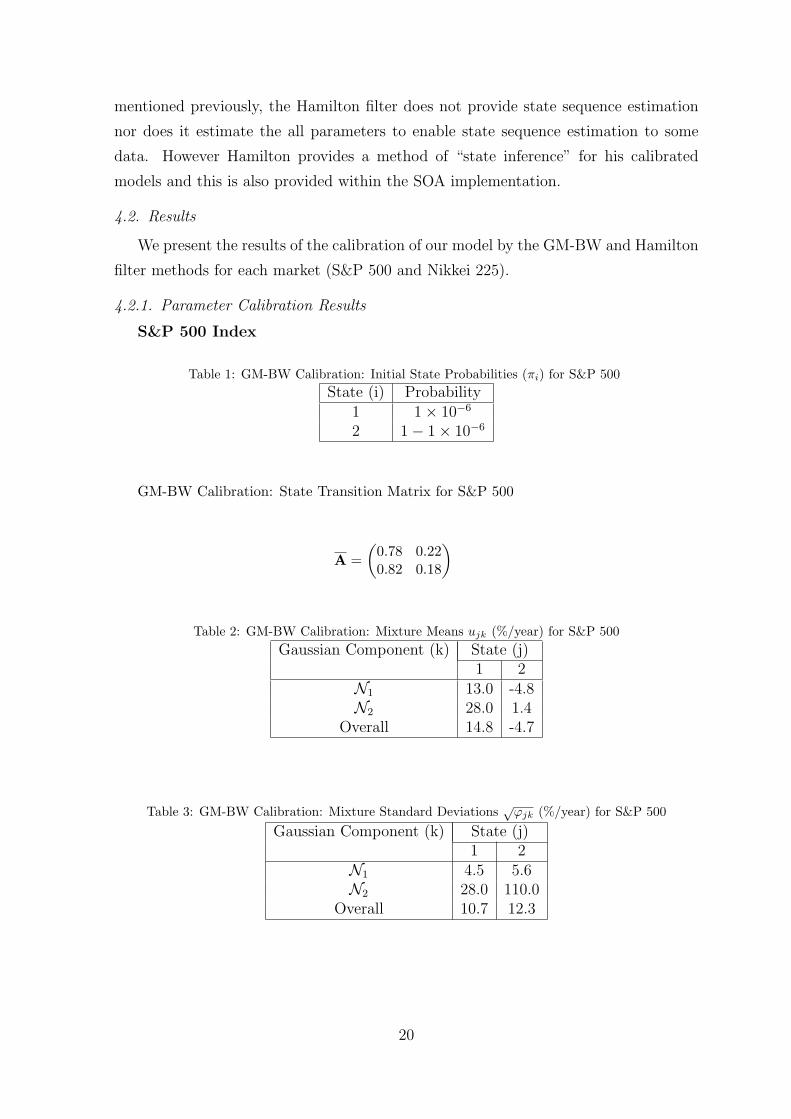
S&P 500 Index

Table 1: GM-BW Calibration: Initial State Probabilities (πi) for S&P 500State (i) Probability

1 1× 10−6

2 1− 1× 10−6

GM-BW Calibration: State Transition Matrix for S&P 500

A =(

0.78 0.220.82 0.18

)

Table 2: GM-BW Calibration: Mixture Means ujk (%/year) for S&P 500Gaussian Component (k) State (j)

1 2N1 13.0 -4.8N2 28.0 1.4

Overall 14.8 -4.7

Table 3: GM-BW Calibration: Mixture Standard Deviations √ϕjk (%/year) for S&P 500

Gaussian Component (k) State (j)1 2

N1 4.5 5.6N2 28.0 110.0

Overall 10.7 12.3

20

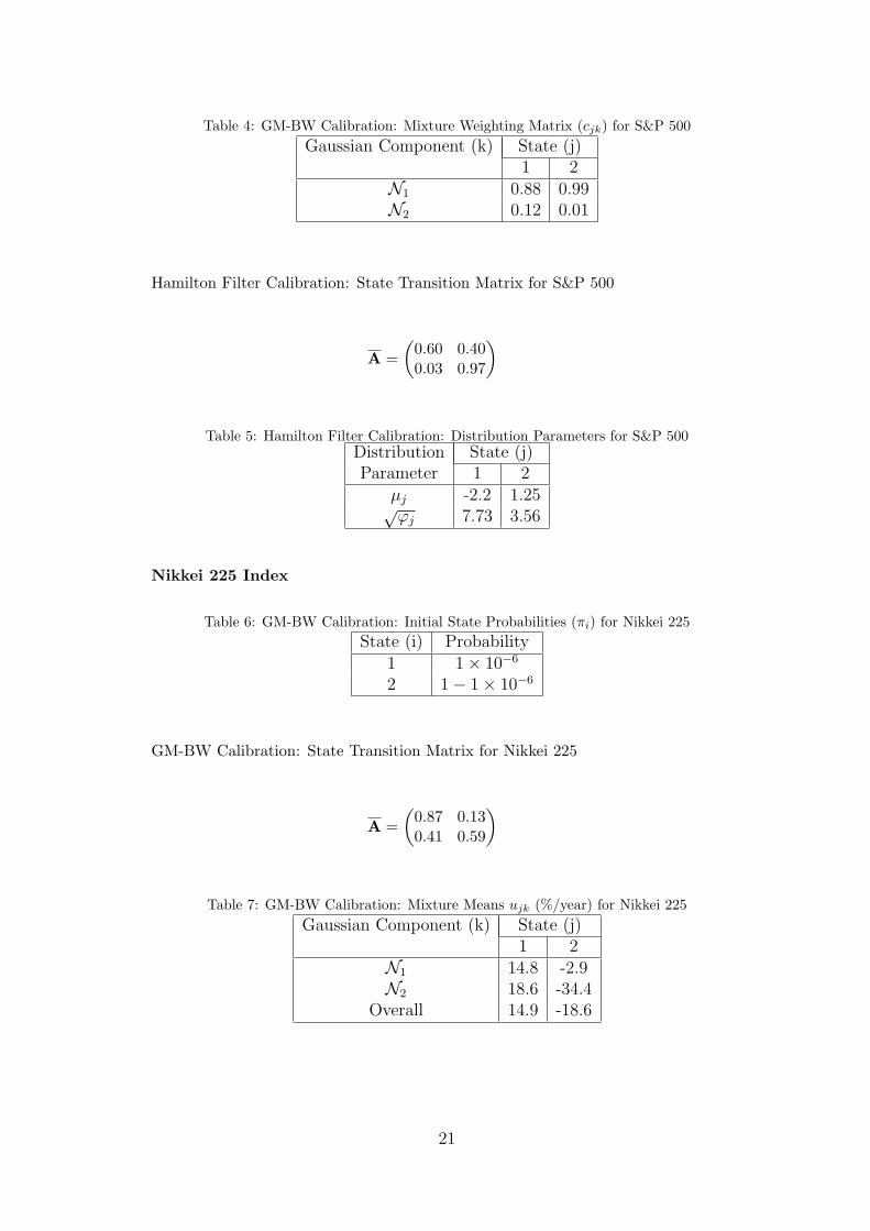
Table 4: GM-BW Calibration: Mixture Weighting Matrix (cjk) for S&P 500Gaussian Component (k) State (j)

1 2N1 0.88 0.99N2 0.12 0.01

Hamilton Filter Calibration: State Transition Matrix for S&P 500

A =(

0.60 0.400.03 0.97

)

Table 5: Hamilton Filter Calibration: Distribution Parameters for S&P 500Distribution State (j)Parameter 1 2

µj -2.2 1.25√ϕj 7.73 3.56

Nikkei 225 Index

Table 6: GM-BW Calibration: Initial State Probabilities (πi) for Nikkei 225State (i) Probability

1 1× 10−6

2 1− 1× 10−6

GM-BW Calibration: State Transition Matrix for Nikkei 225

A =(

0.87 0.130.41 0.59

)

Table 7: GM-BW Calibration: Mixture Means ujk (%/year) for Nikkei 225Gaussian Component (k) State (j)

1 2N1 14.8 -2.9N2 18.6 -34.4

Overall 14.9 -18.6

21

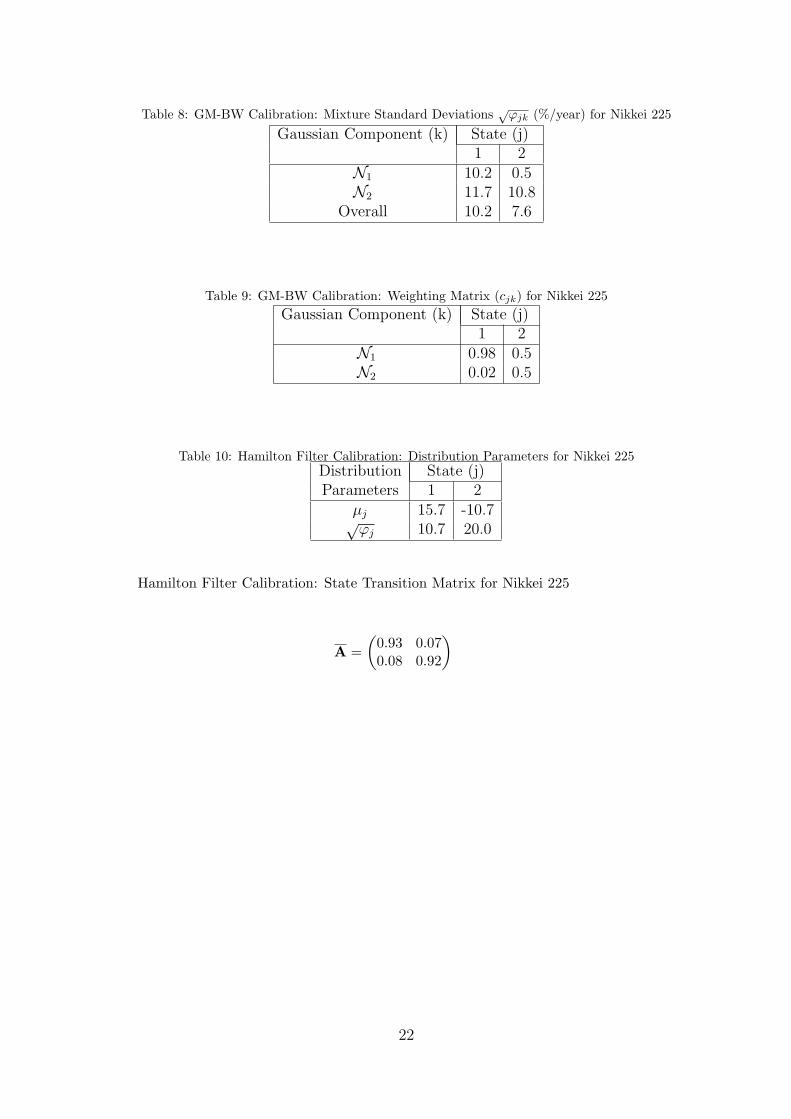
Table 8: GM-BW Calibration: Mixture Standard Deviations √ϕjk (%/year) for Nikkei 225

Gaussian Component (k) State (j)1 2

N1 10.2 0.5N2 11.7 10.8

Overall 10.2 7.6

Table 9: GM-BW Calibration: Weighting Matrix (cjk) for Nikkei 225Gaussian Component (k) State (j)

1 2N1 0.98 0.5N2 0.02 0.5

Table 10: Hamilton Filter Calibration: Distribution Parameters for Nikkei 225Distribution State (j)Parameters 1 2

µj 15.7 -10.7√ϕj 10.7 20.0

Hamilton Filter Calibration: State Transition Matrix for Nikkei 225

A =(

0.93 0.070.08 0.92

)

22

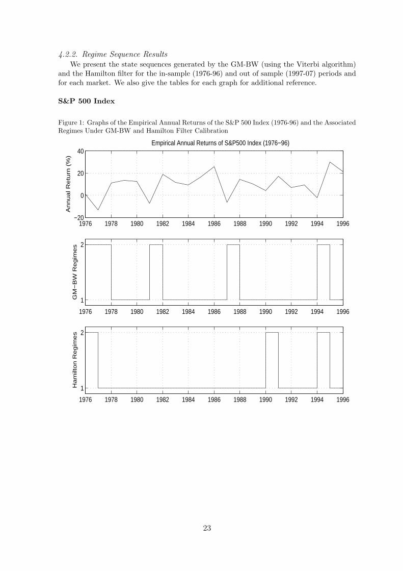
4.2.2. Regime Sequence ResultsWe present the state sequences generated by the GM-BW (using the Viterbi algorithm)

and the Hamilton filter for the in-sample (1976-96) and out of sample (1997-07) periods andfor each market. We also give the tables for each graph for additional reference.

S&P 500 Index

Figure 1: Graphs of the Empirical Annual Returns of the S&P 500 Index (1976-96) and the AssociatedRegimes Under GM-BW and Hamilton Filter Calibration

1976 1978 1980 1982 1984 1986 1988 1990 1992 1994 1996−20

0

20

40Empirical Annual Returns of S&P500 Index (1976−96)

An

nu

al R

etu

rn (

%)

1976 1978 1980 1982 1984 1986 1988 1990 1992 1994 1996

1

2

GM

−B

W R

eg

ime

s

1976 1978 1980 1982 1984 1986 1988 1990 1992 1994 1996

1

2

Ha

milt

on

Re

gim

es

23

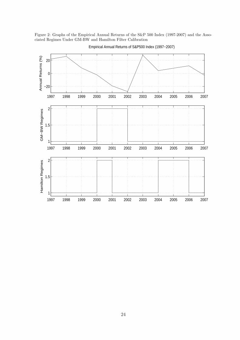
Figure 2: Graphs of the Empirical Annual Returns of the S&P 500 Index (1997-2007) and the Asso-ciated Regimes Under GM-BW and Hamilton Filter Calibration

1997 1998 1999 2000 2001 2002 2003 2004 2005 2006 2007

−20

0

20

Empirical Annual Returns of S&P500 Index (1997−2007)

An

nu

al R

etu

rns (

%)

1997 1998 1999 2000 2001 2002 2003 2004 2005 2006 2007

1

1.5

2

GM

−B

W R

eg

ime

s

1997 1998 1999 2000 2001 2002 2003 2004 2005 2006 2007

1

1.5

2

Ha

milt

on

Re

gim

es

24

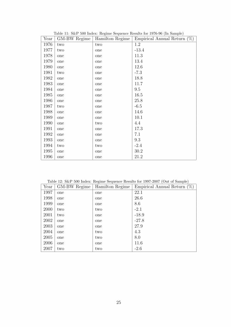
Table 11: S&P 500 Index: Regime Sequence Results for 1976-96 (In Sample)Year GM-BW Regime Hamilton Regime Empirical Annual Return (%)1976 two two 1.21977 two one -13.41978 one one 11.31979 one one 13.41980 one one 12.61981 two one -7.31982 one one 18.81983 one one 11.71984 one one 9.51985 one one 16.51986 one one 25.81987 two one -6.51988 one one 14.61989 one one 10.11990 one two 4.41991 one one 17.31992 one one 7.11993 one one 9.31994 two two -2.41995 one one 30.21996 one one 21.2

Table 12: S&P 500 Index: Regime Sequence Results for 1997-2007 (Out of Sample)Year GM-BW Regime Hamilton Regime Empirical Annual Return (%)1997 one one 22.11998 one one 26.61999 one one 8.62000 two two -2.12001 two one -18.92002 one one -27.82003 one one 27.92004 one two 4.32005 one two 8.02006 one one 11.62007 two two -2.6

25

Nikkei 225 Index

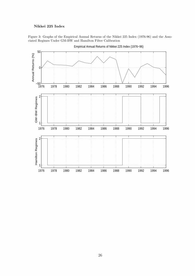
Figure 3: Graphs of the Empirical Annual Returns of the Nikkei 225 Index (1976-96) and the Asso-ciated Regimes Under GM-BW and Hamilton Filter Calibration

1976 1978 1980 1982 1984 1986 1988 1990 1992 1994 1996−50

0

50

Empirical Annual Returns of Nikkei 225 Index (1976−96)

An

nu

al R

etu

rns (

%)

1976 1978 1980 1982 1984 1986 1988 1990 1992 1994 1996

1

2

GM

−B

W R

eg

ime

s

1976 1978 1980 1982 1984 1986 1988 1990 1992 1994 1996

1

2

Ha

milt

on

Re

gim

es

26

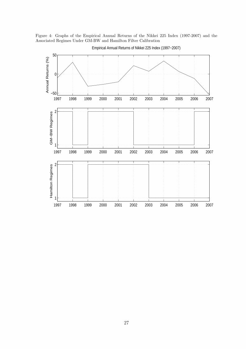
Figure 4: Graphs of the Empirical Annual Returns of the Nikkei 225 Index (1997-2007) and theAssociated Regimes Under GM-BW and Hamilton Filter Calibration

1997 1998 1999 2000 2001 2002 2003 2004 2005 2006 2007−50

0

50

An

nu

al R

etu

rns (

%)

1997 1998 1999 2000 2001 2002 2003 2004 2005 2006 2007

1

2

Empirical Annual Returns of Nikkei 225 Index (1997−2007)G

M−

BW

Re

gim

es

1997 1998 1999 2000 2001 2002 2003 2004 2005 2006 2007

1

2

Ha

milt

on

Re

gim

es

27

Table 13: Nikkei 225 Index: Regime Sequence Results for 1976-96 (In Sample)Year GM-BW Regime Hamilton Regime Empirical Annual Return (%)1976 two two -2.51977 one one 21.01978 one one 9.01979 one one 8.01980 one one 7.61981 one one 4.31982 one one 21.01983 one one 15.41984 one one 12.81985 one one 35.51986 one one 14.21987 one one 33.51988 one one 25.51989 two two -49.01990 two two -3.71991 two two -30.61992 one two 2.91993 one two 12.41994 one two 0.71995 two two -2.61996 two two -23.8

Table 14: Nikkei 225 Index: Regime Sequence Results for 1997-2007 ( Out of Sample)Year GM-BW Regime Hamilton Regime Empirical Annual Return (%)1997 two two -9.71998 one one 31.31999 two two -31.72000 two two -26.82001 two two -20.62002 one two 21.92003 one one 7.32004 one one 33.82005 one one 6.72006 two one -11.82007 two one -54.7

28

4.3. Discussion

For the GM-BW method, from tables 2 and 7 we can infer that the method has attributedstate two as the down state since their overall means are negative, unlike state one. This isalso consistent with the state sequences generated in the S&P 500 and Nikkei 225 markets(see figures 1-4). Furthermore the initial state probabilities π for both markets suggest thatwe start 1976 in state 2. This is consistent with the empirical data where the 1976 returnsare low: for the S&P 500 and Nikkei 225 it is 1.2% and -2.5% respectively (see tables 11 and13).

The GM-BW transition matrices A capture the differing time dynamics for each market,which one can observe from the empirical returns in figures 1 and 3. For the S&P 500 market1976-96 we can see the annual returns exhibit an approximate cyclical relation with a cycletime of 5 years (average life time of an economic cycle). The GM-BW S&P 500 A capturesthis reversionary dynamic through the probability 0.82 of returning to state 1, given we arein state 2. The Nikkei market from 1976-96 on the other hand tends not to exhibit cyclicalbehaviour, rather tends to remain in its current state (be it state 1 or 2). Hence the diagonaltransition probabilities (which capture the memory effect of returning to the same state) arehigher for the Nikkei than in the S&P 500. In conclusion, the GM-BW parameter estimates(distribution and HMM parameters) are consistent with each other and consistent with theempirical data in both markets.

For the Hamilton filter calibration, the calibrated models were less consistent than theGM-BW models. As one can see from tables 5 and 10 the filter has given state one a positivemean for the Nikkei 225 market but not for the S&P 500. Since state one is meant torepresent the up state it should have a positive mean in both markets, hence the Hamiltoncalibration has not been as satisfactory. Note that we could have assigned state one asthe down state for the Hamilton filter, however this would have produced regime sequencesextremely inconsistent with the empirical data (see figures 1-4).

The Hamilton filter produces state transition matrices that are less consistent with theempirical data. Firstly, as explained previously the S&P 500 exhibits cyclical behaviour,which was successfully captured by the GM-BW’s transition matrix, for example the proba-bility of returning to state one given we are in state 2 is 0.82. However for the same transitionprobability the Hamilton filter only assigns a probability of 0.03, which implies the modelshould not cycle or quickly revert back to state 1. The Hamilton filter model also implies thatthe S&P 500 market has a probability of 0.97 remaining in state 2 given it is in state 2, yetthe empirical returns clearly do not remain stuck in a down state. Secondly, the Hamiltonfilter for the Nikkei market assigns a probability of 0.92 to state 2, given we are in state 2, sothat the model remains depressed in state 2 once it enters it. However the empirical returnsof the Nikkei 1976-96 market (see figure 3) shows the market returns fluctuate.

To compare the quality of the models against the empirical data, regime sequences wereproduced from the GM-BW and Hamilton filter models for the in sample and out of sampleperiods. For the GM-BW model one can see from figures 1 and 3 the regime switchescorrespond well to the in sample empirical data: the model switches to state 2 during lowreturns and state 1 otherwise for both markets. The Hamilton filter on the other hand (forthe in sample period) incorrectly identifies regimes for some years. For the S&P 500, theHamilton filter identifies state one for years with significant negative returns rather than asstate 2: 1977 (-13.4%), 1981 (-7.3%) and 1987 (-6.5%). Similarly for the Nikkei market theHamilton filter identifies 1994 as state 2 (7.1%) rather than state 1. Overall, the Hamiltonfilter tends to incorrectly identify states more than the GM-BW method for the in sampleperiod.

In the out of sample period (1997-07), regime sequencing performance of the GM-BWtends to outperform the Hamilton filter. For both markets the GM-BW model accurately

29

identifies the states for most years (see figures 2 and 4) e.g. for the S&P 500 for 2000-2 wasthe period of the “internet bubble crash” and is identified as state 2 by GM-BW. Howeverthe Hamilton filter model does not identify 2001 as state 2 (see figure 2) despite the highlynegative return (-18.9%), nor the following years as state 1 despite the positive returns: 2004(4.3%) and 2005 (8%). Similarly for the Nikkei market the GM-BW accurately identifies thestate of the market whereas the Hamilton identifies 2006 and 2007 as state 1 when they havehighly negative returns -11.8% and -54.7% respectively. In conclusion we can say that theGM-BW calibration method outperforms the Hamilton filter for both markets, in and out ofsample, in terms of parameter model estimation and regime sequence identification.

5. Conclusions

This paper has shown the advantages of Baum-Welch calibration over standard Hamiltonfilter method for calibration of regime switching volatility models. Not only does the Baum-Welch method offer a complete calibration procedure but also is able to estimate the full setof HMM parameters, unlike the Hamilton filter. We have also validated the usage of theBaum-Welch method through numerical experiments on S&P 500 and Nikkei 225 index data,in and out of sample, and compared its performance against the Hamilton filter.

30

References

[A.H00] A.Holtsberg. A statistics toolbox for matlab and octave.http://www.maths.lth.se/matstat/stixbox/, 2000.

[AK08] C. Alexander and A. Kaeck. Regime dependent determinants of credit defaultswap spreads. Journal of Banking and Finance, 32(6):637–648, 2008.

[BEDE04] P. Boufounos, S. El-Difrawy, and D. Ehrlich. Basecalling using hidden Markovmodels. Journal of the Franklin Institute, 341(1-2):23–36, 2004.

[BHL06] G. Bekaert, C.R. Harvey, and C. Lundblad. Growth volatility and financialliberalization. Journal of International Money and Finance, 25(3):370–403, 2006.

[BLR06] L. Bauwens, S. Laurent, and J.V.K. Rombouts. Multivariate GARCH Models:A Survey. Journal of Applied Econometrics, 21(1):79–109, 2006.

[BR02] C. Brooks and A.G. Rew. Testing for non-stationarity and cointegration allowingfor the possibility of a structural break: an application to EuroSterling interestrates. Economic Modelling, 19(1):65–90, 2002.

[BSS07] I. Buckley, D. Saunders, and L. Seco. Portfolio optimization when asset returnshave the Gaussian mixture distribution. European Journal of Operational Re-search, 185(3):1434–1461, 2007.

[DM94] J.M. Durland and T.H. McCurdy. Duration-Dependent Transitions in a MarkovModel of US GNP Growth. Journal of Business and Economic Statistics,12(3):279–288, 1994.

[EvdH97] R.J. Elliott and J. van der Hoek. An application of hidden Markov models toasset allocation problems. Finance and Stochastics, 1(3):229–238, 1997.

[Fam65] E.F. Fama. The behaviour of stock market prices. Journal of Business, 38(1):34–105, 1965.

[FJ73] G.D. Forney Jr. The Viterbi algorithm. Proceedings of the IEEE, 61(3):268–278,1973.

[Ham89] J.D. Hamilton. A New Approach to the Economic Analysis of NonstationaryTime Series and the Business Cycle. Econometrica, 57(2):357–384, 1989.

[Ham91] J.D. Hamilton. A Quasi-Bayesian Approach to Estimating Parameters for Mix-tures of Normal Distributions. Journal of Business & Economic Statistics,9(1):27–39, 1991.

[Ham94] J.D. Hamilton. Time series analysis. Princeton, 1994.

[Har01] M.R. Hardy. A Regime-Switching Model of Long-Term Stock Returns. NorthAmerican Actuarial Journal, 5(2):41–53, 2001.

[Hon03] T. Honda. Optimal portfolio choice for unobservable and regime-switching meanreturns. Journal of Economic Dynamics and Control, 28(1):45–78, 2003.

[HS94] J.D. Hamilton and R. Susmel. Autoregressive Conditional Heteroskedasticity andChanges in Regime. Journal of Econometrics, 64(1-2):307–33, 1994.

31

[JR91] B.H. Juang and L.R. Rabiner. Hidden Markov models for speech recognition.Technometrics, 33(3):251–272, 1991.

[KY95] M.J. Kim and J.S. Yoo. New index of coincident indicators: A multivariateMarkov switching factor model approach. Journal of Monetary Economics,36(3):607–630, 1995.

[LDLK04] N. Liu, R.I.A. Davis, B.C. Lovell, and P.J. Kootsookos. Effect of initial HMMchoices in multiple sequence training for gesture recognition. Information Tech-nology: Coding and Computing, 1(1):5–7, 2004.

[Lev05] S.E. Levinson. Mathematical Models for Speech Technology. Wiley England, 2005.

[MGPG06] C. Melodelima, L. Gueguen, D. Piau, and C. Gautier. A computational predictionof isochores based on hidden Markov models. Gene, 385(1):41–49, 2006.

[Mit09a] S. Mitra. A Review of Volatility and Option Pricing. Arxiv, 2009.

[Mit09b] S. Mitra. Regime Switching Stochastic Volatility with Perturbation Based OptionPricing. Arxiv, 2009.

[MT07] E. Messina and D. Toscani. Hidden Markov models for scenario generation. IMAJournal of Management Mathematics, 19(4):379–401, 2007.

[Mur08] K. Murphy. Hidden markov model (hmm) toolbox for matlab.http://www.cs.ubc.ca/ murphyk/Software/HMM/hmm.html, 2008.

[PS98] Z. Psaradakis and M. Sola. Finite-sample properties of the maximum likelihoodestimator in autoregressive models with Markov switching. Journal of Econo-metrics, 86(2):369–386, 1998.

[Rab89] L.R. Rabiner. A tutorial on hidden Markov models and selected applications inspeech recognition. Proceedings of the IEEE, 77(2):257–286, 1989.

[Rab08] L.R. Rabiner. Private Communication, 2008.

[RI02] A. Ridolfi and J. Idier. Penalized Maximum Likelihood Estimation for Nor-mal Mixture Distributions. School of Computer and Information Sciences, EcolePolytechnique Federale de Lausanne, 200285, 2002.

[Sch89] G.W. Schwert. Why Does Stock Volatility Change Over Time? Journal ofFinance, 44(5):1115–1153, 1989.

[SF06] T. Salih and K. Fidanboylu. Modeling and analysis of queuing handoff calls insingle and two-tier cellular networks. Computer Communications, 29(17):3580–3590, 2006.

[SSS02] M. Sola, F. Spagnolo, and N. Spagnolo. A test for volatility spillovers. EconomicsLetters, 76(1):77–84, 2002.

[TG01] E. Trentin and M. Gori. A survey of hybrid ANN/HMM models for automaticspeech recognition. Neurocomputing, 37(1-4):91–126, 2001.

[Tim00] A. Timmermann. Moments of Markov switching models. Journal of Economet-rics, 96(1):75–111, 2000.

32

[TK84] H.M. Taylor and S. Karlin. An introduction to stochastic modeling. AcademicPress San Diego, 1984.

[VPHS04] P.L. Valls-Pereira, S. Hwang, and S.E. Satchell. How persistent is volatility?An answer with stochastic volatility models with Markov regime switching stateequations. Journal of Business Finance and Accounting, 34(5-6):1002–1024, 2004.

33