Regime Switching Model of US Crude Oil and Stock Market Prices:

1859 to 2013

Mehmet Balcilar Department of Economics

Eastern Mediterranean University Famagusta, NORTHERN CYPRUS, via Mersin 10, TURKEY

Rangan Gupta

Department of Economics University of Pretoria

Pretoria, 0002, SOUTH AFRICA

Stephen M. Miller* Department of Economics,

University of Nevada, Las Vegas Las Vegas, Nevada, 89154-6005 USA

E-mail: stephen.miller@unlv.edu Telephone: 01-702-895-3969

Fax: 01-702-895-1354

Abstract:

This paper examines the relationship between US crude oil and stock market prices, using a Markov-Switching vector error-correction model and a monthly data set from 1859 to 2013. The sample covers the entire modern era of the petroleum industry, which typically begins with the first drilled oil well in Titusville, Pennsylvania in 1858. We estimate a two regime model that divides the sample into high- and low-volatility regimes based on the variance-covariance matrix of the oil and stock prices. We find that the high-volatility regime more frequently exists prior to the Great Depression and after the 1973 oil price shock caused by the Organization of Petroleum Exporting Countries. The low-volatility regime occurs more frequently when the oil markets fell largely under the control of the major international oil companies from the end of the Great Depression to the first oil price shock in 1973. Using the National Bureau of Economic research business cycle dates, we also find that the high-volatility regime more likely occurs when the economy experiences a recession.

Keywords: Markov switching, vector error correction, oil and stock prices JEL classification: C32, E37

* Corresponding author

1

1. Introduction

Macroeconomic policymakers consider wealth as an important driver of the economy and

view asset prices as important predictors of the business cycle. For example, researchers have

long followed the stock market in the US as an important predictor of the business cycle.

(Moore 1983; Siegel 1991; Chauvet 1998-1999). For example, Siegel (1991) determines that

for the 41 recessions observed since 1802, at least an 8-percent loss in stock returns preceded

38. On the negative side, 12 false signals occurred using this criterion, where no recession

followed. Seven of these false signals happened after WWII. Other researchers consider the

predictive ability of crude oil prices. Hamilton (2003, 2009) argues that oil price shocks

proximately cause post-WWII recessions in the US.1

The existing literature contains several attempts to identify the effects of changes in

crude oil prices on certain macroeconomic variables, such as, real GDP growth rates,

inflation, employment, and exchange rates (Hamilton, 1983; Gisser and Goodwin, 1986;

Mork, 1989; Hooker, 1996; Davis and Haltiwanger, 2001, Hamilton and Herrera, 2002, Lee

and Ni, 2002; Hooker, 2002, and so on). These research papers differ from each other and do

not produce a general consensus.

Fewer research papers examine the relationship between crude oil prices and other

asset prices, such as stock prices or stock returns. Market participants want a framework that

identifies how oil-price changes affect stock prices or stock market returns. On theoretical

grounds, oil-price shocks affect stock market returns or prices through their effect on

expected earnings (Jones et al., 2004). The relevant literature includes the following studies.

Kaul and Seyhun (1990) and Sadorsky (1999) report a negative effect of oil-price volatility

1 Even other views exist, however. For example, Leamer (2007) argues that “housing is the business cycle,” showing that significant declines in housing construction preceded 8 of the last 10 recessions. Iacoviello and Neri (2010) estimate a DSGE model and consider the role of the housing market in the propagation of the business cycle. They conclude that “… spillovers from the housing market to the broader economy are non-negligible, concentrated on consumption rather than business investment, and have become more important over time, …” (p. 57).

2

on stock prices. Jones and Kaul (1996) show that international stock prices do react to oil

price shocks. Huang et al. (1996) provide evidence in favor of causality effects from oil

futures prices to stock prices. More recently, Faff and Brailsford (2000) report that oil-price

risk proved equally important to market risk, in the Australian stock market. Hong et al.

(2004) also identify a negative association between oil-price returns and stock-market

returns. Pollet (2005) and Driesprong et al. (2008) find that oil-price changes predict stock

market returns on a global basis, while Hammoudeh and Li (2004) and Hammoudeh and

Eleisa (2004) also discover the importance of the oil factor for stock prices in certain oil-

exporting economies. Bittlingmayer (2005) documents that oil-price changes associate with

war risk and those associated with other causes exhibit an asymmetric effect on the behavior

of stock prices. Sawyer and Nandha (2006), however, using a hierarchical model of stock

returns, report results against the importance of oil prices on aggregate stock returns, while

they retain their explanatory power only on an industrial (sectoral) level. Finally, Gogineni

(2008) also provides statistical support for a number of hypotheses, such as oil prices

positively associate with stock prices, if oil price shocks reflect changes in aggregate demand,

but negatively associate with stock prices, if they reflect changes in supply. Moreover, stock

prices respond asymmetrically to changes in oil prices.

Recently, however, researchers began asking whether changes in macroeconomic

variables cause oil price changes, leading to the decomposition of those oil price changes into

the structural shocks hidden behind such changes (Kilian, 2008a; Kilian and Park, 2009).

That is, different sources of oil price changes may imply non-uniform effects on certain

macroeconomic variables. More specifically, the relevant literature generates mixed views

regarding the effect of such oil-price shocks on asset prices, such as stock prices. Chen et al.

(1986) argue that oil prices do not affect the trend of stock prices, while Jones and Kaul

3

(1996) present evidence that favors a negative association. This negative relationship,

however, does not receive support by Huang et al. (1996) and Wei (2003).

Kilian (2008a) criticizes all these analyses, because researchers treat oil-price shocks

as exogenous. Certain work, however, argues that oil prices respond to factors that also affect

stock prices (Barsky and Kilian 2002, 2004; Hamilton 2005; Kilian 2008b). Thus, researchers

must decompose aggregate oil price shocks into the structural factors that reflect the

endogenous character of such shocks.

Thus, this paper investigates the relationship between the Standard and Poor’s S&P

500 (SP500) stock market index and the West Texas Intermediate (WTI) spot crude oil price

from September 1859 through December 2013, using a Markov-switching vector error-

correction (MS-VEC) model. The MS-VEC model includes two regimes -- high- and low-

volatility regimes. One unique feature of our analysis is that the sample period runs from the

beginning of the modern era of the petroleum industry with the drilling of the first oil well in

the US at Titusville, Pennsylvania in 1958.

Our findings imply that the high-volatility regime more frequently existed prior to the

Great Depression and after the 1973 oil price shock caused by the Organization of Petroleum

Exporting Countries (OPEC). The low-volatility regime occurred more frequently during the

period of time from the end of the Great Depression to the first OPEC oil price shock, where

the oil markets fell largely under the control of the major international oil companies. We

also find a proclivity for the high-volatility regime to occur when the economy experiences a

recession.

The paper unfolds as follows. Section 2 outlines the methodology used in the analysis.

Section 3 implements the several steps in estimating the MS-VEC – data description, unit-

root tests, cointegration tests, MS-VEC estimation, calculation of smoothed probabilities of

4

the high-volatility regime, and impulse response analysis -- and discusses the findings.

Section 4 concludes.

2. Methodology

Conventional wisdom suggests that macroeconometric time-series models must address

structural change and/or regime shift (see Granger, 1996). Indeed, the survey paper by

Hansen (2001) or Perron (2006) affirm that econometric applications should distinctly

consider regime shifts.

Econometricians recently developed new models that can tackle sufficiently certain

types of structural changes. One appealing, the Markov switching (MS) approach proposed

by Hamilton (1990) and later extended to multivariate time-series models by Krolzig (1997,

1999), can address structural breaks. Hamilton (1990) introduced univariate Markov

switching autoregressive (MS-AR) model while Krolzig (1997, 1999) developed multivariate

extensions to Markov switching vector autoregressive (MS-VAR) and Markov switching

vector error correction (MS-VEC) models. The MS models fall within the category of

nonlinear time-series models that emerge from nonlinear dynamic processes, such as high-

moment structures, time-varying parameter, asymmetric cycles, and jumps or breaks in a time

series (Fan and Yao, 2003). The long sample period includes several influential prior events,

such as the Panic of 1907, the Great Depression, World War I and II, first and second OPEC

oil-price shocks, and more recently the global financial crisis and Great Recession of 2008.

The data also includes a significant number of influential business cycles. MS models can

provide a good fit to such time series data with business cycles features and regime shifts.

Several studies successfully use MS models to analyze aggregate output and business

cycles (e.g., Hamilton 1989; Diebold, et al. 1994; Durland and McCurdy 1994; Filardo 1994,

Ghysels 1994; Kim and Yoo 1995; and Filardo and Gordon 1998). Numerous studies also

utilize MS models in the context of stock market returns (e.g. Tyssedal and Tjostheim 1988;

5

Schwert 1989; Pagan and Schwert 1990; Kim, et al. 1998; and Kim and Nelson, 1998).

Following these studies, we consider the MS-VEC model, which, with its rich structure, can

accommodate the dynamic features of oil and stock price data in our sample. The model

choice unlike other traditional models not only efficiently captures the dynamics of the

process in a co-integration space, but also possesses an appealing structural form and

provides economically intuitive results.

The method chosen uses a vector-error correction (VEC) model with time-varying

parameters where, given our objectives, the parameter time-variation directly reflects regime

switching. In this approach, we treat changes in the regimes as random events governed by an

exogenous Markov process, leading to the MS-VEC model. A latent Markov process

determines the state of the economy, where the probability of the latent state process takes a

certain value based on the sample information. In this model, inferences about the regimes

reflects the estimated probability, which measures the probability of each observation in the

sample coming from a particular regime. The MS-VEC model analyzes the time-varying

dynamic relationship between the monthly spot crude oil and stock prices and extends the

class of autoregressive models studied in Hamilton (1990) and Krishnamurthy and Rydén

(1998). It also permits asymmetric (regime-dependent) inference for impulse response

analysis. The structure of the MS-VEC model comes from the model studied in Krolzig

(1997, 1999). Examples of these models, among others, include Psaradakis et al. (2004),

Krolzig et al. (2002), and Francis and Owyang (2003). Our estimation approach uses the

Bayesian Markov-chain Monte Carlo (MCMC) integration method of Gibbs sampling, from

which we can calculate confidence intervals for the impulse response function of the MS-

VEC model.

6

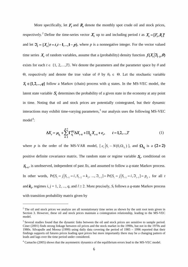
More specifically, let and denote the monthly spot crude oil and stock prices,

respectively.2 Define the time-series vector up to and including period t as

and let , where p is a nonnegative integer. For the vector valued

time series of random variables, assume that a (probability) density function

exists for each t ∈ 1, 2,…,T. We denote the parameters and the parameter space by θ and

Θ, respectively and denote the true value of θ by θ0 ∈ Θ. Let the stochastic variable

follow a Markov (chain) process with q states. In the MS-VEC model, the

latent state variable determines the probability of a given state in the economy at any point

in time. Noting that oil and stock prices are potentially cointegrated, but their dynamic

interactions may exhibit time-varying parameters,3 our analysis uses the following MS-VEC

model4:

(1)

where p is the order of the MS-VAR model, [ (0, )tt t SS Nε Ω ], and is a

positive definite covariance matrix. The random state or regime variable , conditional on

, is unobserved, independent of past Xs, and assumed to follow a q-state Markov process.

In other words, − − − − −= = = ℑ = = = ℑ =1 2 2 1 1 1Pr[ , , ..., ] Pr[ , ]t t t t t t t ijS j S i S k S j S i p , for all t

and , regimes i, j = 1, 2, ..., q, and l ≥ 2. More precisely, St follows a q-state Markov process

with transition probability matrix given by

2 The oil and stock prices we analyze are all nonstationary time series as shown by the unit root tests given in Section 3. However, these oil and stock prices maintain a cointegration relationship, leading to the MS-VEC model. 3 Several studies found that the dynamic links between the oil and stock prices are sensitive to sample period. Ciner (2001) finds strong linkage between oil prices and the stock market in the 1990s, but not in the 1970s and 1980s. Silvapulle and Moosa (1999) using daily data covering the period of 1985 – 1996 reported that their findings supports oil futures prices leading spot prices but more importantly there may be a changing pattern of leads and lags over the time period under considered. 4 Camacho (2005) shows that the asymmetric dynamics of the equilibrium errors lead to the MS-VEC model.

7

11 12 1

11 2

, 1q q

ijj

q q qq

p p pP p

p p p =

= =

∑

. (2)

Thus, pij equals the probability of being in regime j at time t, given that the economy

was in regime i at time (t-1), where i and j take possible values in 1, 2,…, q. This MS-VEC

model allows all parameters, including the variance matrix , to depend on the latent

regime or state variable St.

The matrix contains the long-run relationships between the oil and stock prices in

the MS-VEC model specified in equation (1). We can interpret switching in three ways:

switching in the cointegrating vectors (β'), the weighting matrix (α), or both. Although these

approaches are de facto equivalent, our specification in the error-correction term implies a

single set of long-run relationships and preserves the Engle-Granger notion of cointegration.

We can write the long-run impact matrix as follows:

t tS Sα β′Π = , (3)

where are the state-dependent, long-run impact matrices defined by the ( )n r× matrix of

the state-independent cointegrating vectors β and the ( )n r× state-dependent weighting

matrix .5 In other words, β represents the coefficients of the long-run effects that do not

change over the entire sample period and stands for the regime-dependent adjustment

coefficient that controls how the endogenous variables respond to the disequilibria

represented by the r-dimensional vector 1tXβ −′ . As such, the speed at which the variables

adjust to the long-run equilibrium varies across regimes, which is a key distinction of the

5 Following Krolzig (1997, 1999), we estimate the parameters in the cointegration vector β using the Johansen (1988, 1991) method and imposing one cointegration relationship. These estimates enter the MS-VEC model as predetermined. Our specification assumes constant and regime independent cointegration vectors, while allowing for the presence of the regime-dependent adjustment to the equilibrium. This specification conforms with the nonlinear adjustment to equilibrium examined in Savit (1988).

8

MS-VEC model in equations (1) to (3). For example, a shock in the oil price will exert a

different effect on the stock price depending on whether the economy experiences a low or

high volatility regime. In this model, due to the nonlinear dynamics of the equilibrium

errors,6 denoted by 1t tz Xβ −′= , both the strength with which the equilibrium errors correct

(i.e., ) and the short-run dynamics of the endogenous variables (i.e., ) vary over time.

In our specification, the switches capture differences across regimes in the rate of long-run

adjustment.

In our paper, we assume that two regimes (i.e., q = 2) will sufficiently describe the

dynamic interactions between the oil and stock prices. That is, the two regimes model the

crises-recovery (recession-expansion) cycles observed in many macroeconomic time series.

A large number of studies show that a two-regime MS model proves rich enough to capture

the regime switching behavior in macroeconomic time series (e.g., Hamilton 1988, 1989;

Diebold, et al. 1994; Durland and McCurdy 1994; Filardo 1994, Ghysels 1994; Kim and Yoo

1995; and Filardo and Gordon 1998).

The MS-VEC model in equations (1) to (3) contains several satisfying properties for

analyzing the short-run dynamic interactions of the variables and their responses to

disequilibria. First, we can classify regimes as depending on the parameter switches in the

full sample and, therefore, we can detect changes in dynamic interactions between the

variables. Second, this model allows for many possible changes in the dynamic interactions

between the variables at unknown periods. Third, we can make probabilistic inferences about

the dates at which changes in regimes occur. We can evaluate whether a regime change

actually occurs, and also identify the dates of such regime changes. Finally, we can also use

6 Although the long-run parameters (i.e., β) are state-independent, Camacho (2005) shows that the equilibrium errors follow an MS-VAR model under specifications in equations (1) and (3). Indeed, equation (1) emerges from a model where the equilibrium errors follow an MS-VAR process.

9

this model to drive regime dependent impulse response functions and to determine whether

the effect of an oil price shock on the stock price varies with regimes.

The empirical procedure for building a suitable MS-VEC models starts with

identifying a possible set of models to consider. We determine the order p of the MS-VEC

model using the Bayesian Information Criterion (BIC) in a linear VAR(p) model. The MS-

VEC model specifications may differ in terms of regime numbers (q) and the variance matrix

specification. We only consider regime-dependent (heteroskedastic) variance models,

because both the oil and stock price series span a number of periods where volatilities vary

significantly. Moreover, the actual variances of both oil and stock price series in the high-

volatility regime exceed their respective variances in the low-volatility regime.

Once we identify a specific MS-VEC model, we next test for the presence of

nonlinearities in the data. When testing the MS-VEC model against the linear VEC

alternative, we follow Ang and Bekaert (2002) and use the likelihood-ratio statistic (LR),

which is approximately χ2(q) distributed with q restrictions plus the nuisance parameters (i.e.,

free transition probabilities) that are not identified under the null. We use p-values based on

the conventional χ2 distribution with q degrees of freedom, while for the approximate upper

bound for the significance level of the LR statistic, we use Davies (1987). If we establish

nonlinearity, then we can choose the number of regimes and the type of the MS model based

on both the likelihood-ratio statistic and the Akaike information Criterion (AIC).7

To estimate the MS-VEC model, we adopt a two-step procedure due to Krolzig

(1997), Saikkonen (1992), Saikkonen and Luukkonen (1997), and Krolzig, et al. (2002).

Since all variables in the MS-VEC model are stationary, the estimators are asymptotically

normally distributed and the usual statistical inference applies (Krolzig, 1997; Saikkonen,

7 Krolzig (1997) and Psaradakis and Spagnolo (2003) suggest selecting the number of regimes and the MS model using the AIC, and Psaradakis and Spagnolo (2003) show that using Monte Carlo experiment, the AIC generally yields better results in selecting the correct model.

10

1992; Saikkonen and Luukkonen, 1997; Krolzig, et al., 2002). First, we determine the

number of cointegrating relationships using the Johansen (1988, 1991) procedure. We obtain

the equilibrium errors 1t tz Xβ −′= in this first step. Second, we estimate the MS-VEC model

using the determined in the first step. Saikkonen (1992) and Saikkonen and Luukkonen

(1997) show that the Johansen procedure estimates the cointegrating vectors consistently,

even in the presence of regime switching.

Three commonly used methods can estimate the parameters of the MS models. First,

the maximum likelihood (ML), although the simplest method of estimation, proves

computationally demanding and may exhibit slow convergence.8 The ML method faces two

important practical difficulties. One, finding the global maximum of the likelihood function

may prove difficult to locate. Two, the likelihood function for the important class of mixtures

of normal distributions is not bounded and the ML estimator does not exist for the global

maximum.

Second, the more commonly used method of estimation for the MS models is the

expectation maximization (EM) algorithm (Dempster et al. 1977; Lindgren 1978; Hamilton

1990, 1994). Assuming a normal conditional distribution of Xt given 1 0, , ,..., S ; t t tS S θ− ′ℑ ,

the likelihood function is numerically approximated using the EM algorithm in two steps.

One, given the current parameter estimates and the data, we compute the conditional

expectation of log likelihood (E-step), and two, we compute the parameters that maximize the

complete-data log likelihood function (M-step). The EM algorithm may experience slow

convergence and also we cannot directly compute the standard errors of the parameters from

the EM algorithm.

Third, we can use the Bayesian MCMC parameter estimation based on the Gibbs

sampling. The ML and EM methods usually fail for certain types of models, where we cannot 8 Redner and Walker (1984) provide an excellent review of the ML estimation of the MS models.

tz

11

compute the full vector of likelihoods for each regime for each period. The MCMC works

only with one sample path for the regimes rather than a weighted average of sample paths

over all regimes and, therefore, avoids the problem faced by the ML and EM methods.

The MCMC indeed treats the regimes as distinct set of parameter. Our MCMC

implementation uses the following steps:9 (i) Draw the model parameters given the regimes.

In our case, transition probabilities do not enter this step. (ii) Draw the regimes given the

transition probabilities and model parameters. (iii) Draw the transition probabilities given the

regimes. In our case, model parameters do not enter this step.

First, we draw given regimes, P, and using a hierarchical

prior. Our implementation draws a common covariance matrix from the Wishart distribution,

given the inverse of the regime specific covariances. Then, we draw the regime specific

covariances from the inverse Wishart distribution, given the common covariance. The

degrees of freedom priors for Wishart and inverse Wishart distributions both equal 4. We use

a flat prior and draw , given regimes, P, and from a multivariate

Normal distribution with 0 mean.

Second, we draw regimes St given , P, and . This comes

from the Bayes formula, where relative probability of regime i at time t equals the product of

the unconditional regime probability times the likelihood of regime i at time t. We draw

regimes as a random index from 1, …, q, given relative probability weights. That is, we

use the Forward Filter-Backwards Sampling (FFBS) (also called Multi Move Sapling)

algorithm described in Chib (1996) to draw the regimes. Then, we reject any draw, if less

than 5 percent of the observations fall in any of the regimes.

Finally, we draw unconditional probabilities P, given the regimes, from a Dirichlet

distribution. We set the priors for the Dirichlet distribution as 80% probability of staying in 9 See Fruehwirth-Schnatter (2006) for the details of the MCMC estimation of the MS models.

12

the same regime and 20-percent probability of switching to the other regime. We perform the

MCMC integration with 50,000 posterior draws with 20,000 burn-in draws.

We use the impulse response function (IRF) to analyze the dynamic interaction

between the oil and stock price. The IRF analysis studies how a given shock in one variable

propagates to all variables in the system over time (e.g., h = 1, 2, …, H steps after the shock

hits the system). Computing multi-step IRFs from MS-VEC models as well as from all

nonlinear time-series models prove complicated because no ordinary method of computing

the future path of the regime process exists. The IRF analysis requires that we know the

future path of the regime process, since the impulses depend on the system’s regime in every

time period.

Ideally, the IRFs of the MS-VEC model should integrate the regime history into the

propagation period, which proves difficult to resolve. Two approaches work-around the

history dependence of the IRFs in the MS models. Ehrmann et al. (2003) suggest assuming

that regimes do not switch beyond the shock horizon, leading to regime-dependent IRFs

(RDIRF). On the other hand, Krolzig (2006) acknowledges the historical dependence and

allows the regime process to influence the propagation of the shocks for the period of

interest, h=1, 2, … H. In Krolzig’s approach, we compute the conditional probabilities of

future regimes, , given the regime and the transition probabilities, P.

One major attraction of the RDIRF analysis is the possibility of determining the time

variation in the responses of variables to a particular shock. The RDIRF traces the expected

path of the endogenous variable at time t+h after a shock of given size to the k-th initial

disturbance at time t, conditioned on regime i. The k-dimensional response vectors ψki,1,…,

13

ψki,h represents a prediction of the response of the endogenous variables. (Ehrmann et al.

2003). We can define the RDIRFs as follows:10

for h ≥ 0, (4)

where denotes the structural shock to the k-th variable. In general, the reduced-form

shocks will correlate across the equations and will not correspond to . This leads

to the famous identification problem for which several solutions exist. We identify the

structural shocks as . To make structural inferences from the data, we must identify

the structural disturbances and, hence, F. In other words, we impose sufficient restrictions on

the parameter estimates to derive a separate structural form for each regime, from which we

compute the RDIRFs. As standard practice to measure the effect of the oil price on the stock

price, we order the stock price last and use the recursive identification scheme (Sims 1980).

The recursive identification scheme uses the Cholesky decomposition of the covariance

matrix as and identifies structural shocks from with .

The RDIRF analysis, although simple to derive and to construct confidence intervals

via bootstrap, is not appropriate, if regime switching likely occurs during the propagation of

shocks. The Krolzig (2006) solution possesses appeal, but it cannot construct confidence

intervals. In our study, we combine RDIRF analysis with MCMC integration. We examine

whether the dynamic response of the stock price to oil price shocks depends on the state of

the economy, such as crash or recovery periods, assuming a given regime (i.e., regime

switching does occur during the shock propagation periods) and studying the propagation of

the oil price shock in the future, which proves appropriate for our purposes. Building on the

Bayesian impulse responses for the linear VAR models (Ni et al. 2007), we drive the 10 Refer to Ehrmann et al. (2003) for details on characteristics and computation of the regime-dependent impulse responses.

14

posterior density of the RDIRFs from the Gibbs sampling. The simulations of the posteriors

of the parameters jointly with the identification of the structural shocks via the Gibbs sampler

directly yield the posterior densities of the RDIRFs. We compute the confidence bands by the

MCMC integration with Gibbs sampling of 50,000 posterior draws with a burn-in of 20,000.

3. Data and Empirical Findings

3.1. Data

We collected data on the Standard and Poor’s S&P 500 (SP500) stock market index, and

West Texas Intermediate (WTI) spot crude oil price from September 1859 through December

2013 for 1,852 observations. Data come from the Global Financial Database. We seasonally

adjust the data using Census X13. Figure 1 plots the natural logarithm of the two series. The

shaded (grey) bars identify the National Bureau of Economic Research (NBER) recessions in

the US economy. Frequently, the SP500 and the WTI fall during recessions, although not in

every recession.

Table 1 reports the descriptive statistics for the natural logarithms of the SP500 and

WTI series in Panel A. Panel B gives the descriptive statistics for SP500 and WTI returns,

measured as the logarithmic difference in the price series. In addition to the mean, standard

deviation (SD), coefficient of variation (CV), minimum (min), maximum (max), skewness,

and kurtosis statistics, the table reports the Jarque-Berra normality test (JB), the Ljung-Box

first [Q(1)] and fourth [Q(4] autocorrelation tests, and the first [ARCH(1)] and fourth

[ARCH(4)] order Lagrange multiplier (LM) tests for autoregressive conditional

heteroskedasticity (ARCH).

For both series in logarithmic levels and logarithmic differences, we reject normality

and find evidence of first- and fourth-order autocorrelation and autoregressive conditional

heteroskedasticity. Using the coefficient of variation to measure relative volatility, we see

15

that the WTI series exhibits more volatility than the SP500 in both logarithmic levels and

logarithmic differences.

The oil price data go back to the first oil well drilled in the US on August 27, 1859 in

Titusville, Pennsylvania, which typically defines the beginning of the modern era in the

petroleum industry. 11 The modern era began in the middle of the 19th Century with the

discovery of how to refine kerosene (and paraffin) from crude oil and the invention of the

kerosene lamp. Kerosine replaced whale oil as the fuel of choice for lamps. The discovery by

Edison of the first commercially practical incandescent light bulb in 1879 led to a phasing out

of kerosene lamps. The invention of a commercially successful internal combustion engine in

1879 boosted the demand for gasoline and other petroleum distillates for transportation

purposes. As we see from Figure 1, the early part of our sample sees boom and bust cycles in

the WTI series. That is, crude oil production and demand experienced significant swings after

the birth of the modern era.

As the petroleum industry matured, price wars amongst the major international

companies in the 1920s led to the 1928 Achnacarry Agreement, which established the

international petroleum cartel (Federal Trade Commission 1952).12 The Agreement divided

markets, fixed prices, restricted production, and limited competition. The fixed prices

supported the profitability of “high-cost” producers of petroleum and the market divisions

and production restrictions attempted to prevent “low-cost” producers from lowering prices

to expand their market shares. The world economy experienced the Great Depression shortly

after the signing of the Achnacarry Agreement, leading to an 86-percent decline in the SP500

11 The first oil well drilled goes back to the middle of the 4th Century in China, using bamboo to drill and to form pipelines. 12 As a precursor to the Achnacarry Agreement, non-US international oil companies signed the Red Line Agreement in 1914 that established the Turkish Petroleum Company (later the Iraq Petroleum Company) whereby these companies agreed not to participate in the crude oil markets in the Ottoman Empire except through the Turkish Petroleum Company. US international oil companies sought admission to this agreement in 1922, finally achieving entry in 1928.

16

index from October 1929 through June 1932 and a 68-percent decline in the WTI price from

January 1929 through May 1933. Figure 1 documents that the WTI price remained relatively

stable from World War II until the effective emergence of OPEC in 1973. That is, although

OPEC formed in 1960, They did not exert significant control over world crude oil prices until

the countries in OPEC nationalized their domestic oil industry. Figure 1 also shows that the

WTI price experiences much more volatility post-1973.

3.2. Unit-root tests

Table 2 Panel A reports unit-root tests for the log levels of the series with a constant and a

linear trend in the test equation. Panel B reports unit-root tests for the first differences of the

log series with only a constant in the test equation. ADF denotes the augmented Dickey-

Fuller (Dickey and Fuller, 1979) test, Zα, the Phillips-Perron Zα unit root test (Phillips and

Perron, 1988), MZα and MZt, the modified Phillips-Perron tests of Perron and Ng (1996),

DF-GLS, the augmented Dickey Fuller test of Elliot et al. (1996) with generalized least

squares (GLS) detrending, KPSS, the Kwiatkowski et al. (1992) stationarity test, and Zivot-

Andrews, the endogenous structural break unit root test of Zivot and Andrews (1992) with

breaks in both the intercept and linear trend. Zα, MZα, and MZt tests depend on GLS

detrending. For the ADF unit root statistic, we select the lag order by sequentially testing the

significance of the last lag at the 10-percent significance level. We select the bandwidth or

the lag order for the MZα, MZt, DF-GLS, and KPSS tests using the modified Bayesian

Information Criterion (BIC)-based data dependent method of Ng and Perron (2001).

In Panel A of Table 2, the KPSS test rejects the null hypothesis of stationary series.

All the other tests cannot reject the null hypothesis of nonstationary series. In Panel B, the

KPSS test cannot reject the null hypothesis of stationary series whereas all other tests reject

the null hypothesis of nonstationary series. In sum, all series test as first-difference stationary

17

series. In sum, we conclude that both the SP500 and WTI series are nonstationary in their

logarithmic differences.

3.3. Multiple cointegration tests

Table 3 reports selection criteria and multivariate cointegration tests for the VAR(p) model of

the natural logarithms of SP500 and WTC. Panel A reports the AIC, BIC, and Hannan-Quinn

(HQ) information criteria. The VAR order of 2 comes from the minimum BIC value. Panel B

reports maximum eigenvalue (λmax) and trace (λtrace) cointegration order tests of Johansen

(1988, 1991). Both the maximum eigenvalue and trace tests support cointegration between

SP500 and WTI. Panel C reports the multivariate cointegration test of Stock and Watson

(1988). Under the null q(k, k-r) of Stock-Watson cointegration test, we test k common

stochastic trends against k-r common stochastic trends (or r cointegration relationships). We

find support for cointegration between SP500 and WTI, using the Stock-Watson test.

3.4. Estimation of MS-VEC model

Table 4 reports estimation results and model selection criteria for the MS-VEC model given

in equations (1) to (3). We select the lag order by the minimum BIC value in a VAR in levels

as 2 for both linear VEC and MS-VEC models. We estimate the MS-VEC model using

Bayesian Monte Carlo Markov Chain (MCMC) method with Gibbs sampling. The MCMC

estimates employ 20,000 burn-in and 50,000 posterior draws. All reported estimates in the

Table for the MS-VEC model come from the Bayesian estimation.

The likelihood ratio statistic tests the linear VEC model under the null against the

alternative MS-VEC model. The LR test is nonstandard, since unidentified parameters exist

under the null. The χ2 p-values (in square brackets) with degrees of freedom equal to the

number of restrictions as well as the number of restrictions plus the numbers of parameters

unidentified under the null reject the null of linearity. The p-value of the Davies (1987) test

18

also rejects linearity. We estimate these models over the full sample period 1959:12-2012:12

with 1849 observations.

The long-run average probabilities of a low and high-volatility regime equal 0.72 and

0.28, respectively. That is, for our 1849 observations, we expect the low- (high-) volatility

regime to occur on 1,334 (515) occasions. These numbers imply an average duration in the

low (high-) volatility regime of 20.7 (8.0) months. The actual outcomes over our sample in

the low- (high-) volatility regime equal 1,279 (570).

3.5. Smoothed probabilities

Figures 2 and 3 plot the estimates of the smoothed probabilities of high volatility regime

(regime 2) of the MS-VEC model given in equations (1) to (3). The smoothed probabilities

equal the means of the 50,000 posterior draws for each time period based on the FFBS

algorithm.

In Figure 2, the shaded (grey) bars correspond the periods where smoothed

probability of the high volatility regime equals or exceeds 0.5. We note that the high

volatility region occurs much more frequently in the pre-1990 era, during the Great

Depression, and in the post 1973 period. Since recessions occur more frequently during the

pre-1990 period, Figure 3 also plots the smoothed probability in regime 2 along with shaded

(grey) bars that correspond to NBER business cycle recession. Visually, Figure 3 seems to

show that a high smoothed probability of a high volatility region associates with a recession,

although not all recessions associate with a high smoothed probability of a high volatility

region. We calculated the average probability of the high volatility region during recessions

and expansions, finding values of 0.49 and 0.28.

If we define high- and low-volatility regimes as 1 and 0, respectively, and recessions

and expansions as 1 and 0, respectively, then we can form a contingency table of outcomes.

Table 5 reports the findings for the entire sample period of 1,849 observations. We soundly

19

reject the χ2 test for independence, which equals 131.45. The odds ratio implies that the

economy is three times more likely to experience a recession in the high-volatility regime

than in the low-volatility regime. In sum, we find a significant relationship between

recessions and a high smoothed probability of the high volatility region

3.6. Impulse response functions

Figure 4 reports 1 to 20 step impulse responses of the stock price to a 1 standard deviation

shock in the oil price. All impulses use the Cholesky factor orthogonalization. Impulses

responses appear as solid lines and the 95-percent confidence intervals appear as dotted lines.

The confidence intervals for the linear VEC model come from 1,000 bootstrap resampling.

The MS-VEC impulse responses are computed using the regime dependent impulse response

method suggested by Ehrmann et al. (2003). The confidence intervals for the MS-VEC

models come from the 50,000 posterior draws.

The impulse responses for the linear VEC model show a significant positive effect of

the oil price shock on the stock price. That is, a positive oil price shock of 1-percent leads to a

growing positive movement in the stock price over time. On the other hand, the impulse

responses during the low- and high-volatility regions show no significant effect and a

significant negative effect, respectively.

Kilian and Park (2009) argue that the linkage between oil and stock prices depends on

the shocks in the oil market. More specifically, shocks to global aggregate demand and

shocks to precautionary demand lead to opposite effects on stock prices. 13 That is, an

unanticipated increase in global demand will raise both oil and stock prices whereas an

increase in precautionary demand will lead to a jump in the oil price and a drop in the stock

price, because uncertainty about future oil supply drives precautionary demand.

13 Kilian and Park (2009) also argue that shocks to oil production prove the least important for explaining stock price movements.

20

Our findings point to the importance of conditioning the linkages on the low- and

high-volatility environments. When we do not differentiate, we find a positive response of

stock prices to a positive shock to oil prices. When we condition on low- and high-volatility

regimes, we find no relationship between the oil price shock and stock prices in the low

volatility regime, supporting the findings of Huang et al. (1996) and Wei (2003), and a

negative relationship for the high-volatility regime, supporting the findings of Jones and Kaul

(1996).

4. Conclusion:

This paper examines the relationship between US crude oil and stock market prices, using a

MS-VEC model and a monthly data set from 1859 to 2013. Our sample period begins at the

time usually identified as the modern era of the petroleum industry, which links to the drilling

of the first oil well in the US at Titusville, Pennsylvania in 1858. The early part of the 20th

century saw the major international oil companies capturing control of the pricing of crude

oil, This control continued until OPEC established its dominance with the nationalization of

domestic oil industries in OPEC countries. That effect control by OPEC saw its initial

success in the first oil price shock of 1973. Since then, OPEC’s power waxed and waned over

time.

We find that the natural logarithms of SP500 stock market index and the WTI crude

oil price series exhibit non-stationary behavior. Moreover, these two series prove

cointegrated, leading to our estimation of the MS-VEC model. We find that the high-

volatility regime more frequently exists prior to the Great Depression and after the 1973 oil

price shock caused by the OPECs. The low-volatility regime occurs more frequently during

the period of time from the end of the Great Depression to the first OPEC oil price shock,

where the oil markets fell largely under the control of the major international oil companies.

21

The impulse-response function analysis in our non-linear model determines that an oil

price shock delivers a negative effect on stock prices for the high-volatility economy,

whereas no relationship exists for the low-volatility economy. Similar analysis in a linear

model produces the opposite finding of a significant positive effect of an oil price shock on

the stock price. This finding suggests that not accounting for nonlinearity can lead to

problematic results. Moreover, the analysis of the linkages between oil and stock prices in the

existing literature does not consider the long sample of observations in our paper, beginning

with the modern era of the petroleum industry through the present. Our analysis opens the

door for additional detailed analysis of the issues across this longer time horizon.

Finally, using the NBER business cycle dates, we examine the relationship between

the smoothed probability of a high-volatility regime and a recession in the macroeconomy.

We find it more likely that the high-volatility regime occurs when the economy experiences a

recession.

References Andrews, D. W. K., 1991. Heteroskedasticity and autocorrelation consistent covariance

matrix estimation. Econometrica 59, 817-858.

Ang, A., Bekaert, G., 2002. International asset allocation with regime shifts. Review of Financial Studies 15, 1137–1187.

Barsky, R. B., Kilian, L., 2002. Do we really know that oil caused the great stagflation? A

monetary alternative. NBER Macroeconomics Annual 2001, 137–183. Barsky, R. B., Kilian, L., 2004. Oil and the macroeconomy since the 1970s. Journal of

Economic Perspectives 18, 115–134. Bittlingmayer, G., 2005. Oil and stocks: Is it war risk? Working Paper Series. University of

Kansas. Camacho, M., 2005. Markov-switching stochastic trends and economic fluctuations. Journal

of Economic Dynamics & Control 29, 135–158. Chauvet. M., (1998-1999). Stock market fluctuations and the business cycle. Journal of

Economic and Social Measurement 25, 235-257.

22

Chib, S., 1996. Calculating posterior distributions and modal estimates in Markov mixture models. Journal of Econometrics 75, 79–97.

Ciner, C., 2001. Energy shocks and financial markets: nonlinear linkages. Studies in Nonlinear Dynamics & Econometrics 5, 203-212.

Davies, R. B., 1987. Hypothesis testing when a nuisance parameter is present only under the

alternative. Biometrika 74, 33-43. Dempster, A. P., Laird, N. M., Rubin, D. B., 1977. Maximum likelihood from incomplete

data via the EM algorithm. Journal of the Royal Statistical Society Series B 34, 1-38. Dickey, D. A., Fuller, W. A., 1979. Distribution of the estimators for autoregressive time

series with a unit root. Journal of the American Statistical Association 74, 427-431. Diebold, F. X., Lee, J.-H., Weinbach, G. C., 1994. Regime switching with time-varying

transition probabilities. In C. Hargreaves (ed.) Nonstationary Time Series Analysis and Cointegration, pp. 283–302, Oxford: Oxford University Press.

Driesprong, G., Jacobsen, B., Benjiman, M., 2008. Striking oil: Another puzzle? Journal of

Financial Economics 89, 307-327 Durland, J. M., McCurdy, T. H., 1994. Duration-dependent transitions in a Markov model of

U.S. GNP growth. Journal of Business and Economic Statistics 12, 279–288. Ehrmann, M., Ellison, M., Valla, N., 2003. Regime-dependent impulse response functions in

a Markov-switching vector autoregression model. Economics Letters 78, 295–299.

Elliott, G., Rothenberg, T. J., Stock, J. H., 1996. Efficient tests for an autoregressive unit root. Econometrica 64, 813–836.

Faff, R., Brailsford, T., 2000. A test of a two-factor ‘market and oil’ pricing model. Pacific

Accounting Review 12 (1), 61–77. Fan, J. Yao, Q., 2003. Nonlinear Time Series: NonparametrPsaric and Parametric Methods.

New York: Springer. Federal Trade Commission, 1952. The International Petroleum Cartel. Staff Report,

submitted to Subcommittee on Monopoly, Select Committee on Small Business, US Senate, 82nd Congress, 2nd session. Washington, DC: U.S. Government Printing Office.

Filardo, A. J., 1994. Business-cycle phases and their transitional dynamics. Journal of

Business and Economic Statistics 12, 299–308. Filardo, A. J., Gordon, S. F., 1998. Business cycle durations. Journal of Econometrics 85,

99–123.

23

Francis, N., Owyang, M., 2003. Asymmetric common trends: An application of monetary policy in Markov-switching VECM. Federal Reserve Bank of St. Louis working paper 2003-001B.

Fruehwirth-Schnatter, S., 2006. Finite Mixture and Markov Switching Models. Statistics.

Springer. Ghysels, E,. 1994. On the periodic structure of the business cycle. Journal of Business and

Economic Statistics 12, 289–298. Gisser, M., Goodwin, T. H., 1986. Crude oil and the macroeconomy: Tests of some popular

notions. Journal of Money, Credit and Banking 18, 95–103. Gogineni, S., 2008. The stock market reaction to oil price changes. Working Paper.

University of Oklahoma. Granger, C. W. J., 1996. Can we improve the perceived quality of economic forecasts?

Journal of Applied Econometrics 11, 455-473. Hamilton, J. D., 1983. Oil and the macroeconomy since World War II. Journal of Political

Economy 9, 228–248. Hamilton, J. D., 1988. A neoclassical model of unemployment and the business cycle.

Journal of Political Economy 96, 593-617. Hamilton, J. D., 1989. A new approach to the economic analysis of nonstationary time series

and the business cycle. Econometrica 57, 357-384. Hamilton, J. D., 1990. Analysis of time series subject to changes in regime. Journal of

Econometrics 45, 39-70. Hamilton, J. D., 1994. Time Series Analysis. Princeton, NJ: Princeton University Press. Hamilton, J. D., 2003. What Is an Oil Shock? Journal of Econometrics 113, 363–398. Hamilton, J. D., 2005. Oil and the macroeconomy, In: Durlauf, S., Blume, L. (Eds.), The New

Palgrave Dictionary of Economics, 2nd Edition. Macmillan, London. Hamilton, J. D., 2009. Causes and Consequences of the Oil Shock of 2007–08. Brookings

Papers on Economic Activity (Spring), 215-261. Hamilton, J. D., Herrera, M. A., 2002. Oil shocks and aggregate macroeconomic behavior.

Journal of Money, Credit and Banking 36, 265–286. Hammoudeh, S., Li, H., 2004. The impact of the Asian crisis on the behavior of US and

international petroleum prices. Energy Economics 26, 135–160. Hammoudeh, S., Eleisa, E., 2004. Dynamic relationships among the GCC stock markets and

the NYMEX oil prices. Contemporary Economic Policy 22, 250–269.

24

Hansen, B. E., 2001. The new econometrics of structural change: dating breaks in U.S. labor productivity. The Journal of Economic Perspectives 15, 117–128.

Hong, H., Torous, W., Valkanov, R., 2004. Do industries lead the stock market? Gradual

diffusion of information and cross-asset return predictability. Working Paper, Stanford University and UCLA.

Hooker, M. A., 1996. What happened to the oil-price macroeconomy relationship? Journal of

Monetary Economics 38, 195–213. Hooker, M. A., 2002. Are oil shocks inflationary? Asymmetric and nonlinear specifications

versus changes in regime. Journal of Money, Credit and Banking 34, 540–561. Huang, R. D., Masulis, R. W., Stoll, H. R., 1996. Energy shocks and financial markets.

Journal of Futures Markets 16, 1–27. Iacoviello M., Neri, S., (2010). Housing market spillovers: Evidence from an estimated

DSGE model. American Economic Journal: Macroeconomics 2(2): 125-164. Johansen, S., 1988. Statistical analysis of cointegration vectors. Journal of Economic

Dynamics and Control 12, 231–254. Johansen, S., 1991. Estimation and Hypothesis Testing of Cointegration Vectors in Gaussian

Vector Autoregressive Models. Econometrica 59, 1551–1580. Jones, C. M., Kaul, G., 1996. Oil and the stock markets. Journal of Finance 51, 463–491. Jones, D. W., Leiby, P. N., Paik, I. K., 2004. Oil price shocks and the macroeconomy: What

has been learned since 1996. Energy Journal 25, 1–32. Kaul, G., Seyhun, N., 1990. Relative price variability, real shocks, and the stock market.

Journal of Finance 45, 479–496. Kilian, L., 2008a. Not all oil price shocks are alike: Disentangling demand and supply shocks

in the crude oil market. American Economic Review 99, 1053-1069.. Kilian, L., 2008b. Exogenous oil supply shocks: How big are they and how much do they

matter for the US economy? Review of Economics and Statistics 90, 216–240. Kilian, L., Park, C., 2009. The impact of oil price shocks on the U.S. stock market.

International Economic Review 50, 1267-1287. Kim, C. J., Nelson, C. R., 1998. Business cycle turning points, a new coincident index, and

tests of duration dependence based on a dynamic factor model with regime switching. Review of Economics and Statistics 80, 188–201.

Kim, C., Nelson, C. R., Startz, R., 1998. Testing for mean reversion in heteroskedastic data

based on Gibbs-sampling-augmented randomization. Journal of Empirical Finance 5, 131-154.

25

Kim, M.-J., Yoo, J.-S., 1995. New index of coincident indicators: A multivariate Markov switching factor model approach. Journal of Monetary Economics 36, 607– 630.

Krishnamurthy, V., Rydén, T., 1998. Consistent estimation of linear and non-linear

autoregressive models with Markov regime. Journal of Time Series Analysis 19, 291-307.

Krolzig, H.-M., 1997. Markov Switching Vector Autoregressions Modelling: Statistical

Inference and Application to Business Cycle Analysis. Berlin: Springer. Krolzig, H.-M., 1999. Statistical analysis of cointegrated VAR processes with Markovian

regime shifts. Working Paper # 1113, Computing in Economics and Finance 1999, Society for Computational Economics.

Krolzig, H.-M., 2006. Impulse response analysis in Markov switching vector autoregressive

models. Economics Department, University of Kent. Keynes College.

Krolzig, H.-M., Marcellino, M., Mizon, G. E., 2002. A Markov-switching vector equilibrium correction model of the UK labor market. Empirical Economics 27, 233-254.

Kwiatkowski, D., Phillips, P., Schmidt, P., Shin, J., 1992. testing the null hypothesis of

stationarity against the alternative of a unit root. Journal of Econometrics 54, 159–178.

Leamer, E. E., (2007). Housing is the business cycle. In Housing, Housing Finance, and

Monetary Policy, Economic Symposium Conference Proceedings, Kansas City Federal Reserve Bank, 149-233.

Lee, K., Ni, S., 2002. On the dynamic effects of oil shocks: A study using industry level data.

Journal of Monetary Economics 49, 823–852. Lindgren, G., 1978. Markov regime models for mixed distributions and switching

regressions. Scandinavian Journal of Statistics 5, 81-91. Moore, G. H., (1983). Security markets and business cycles. In Business Cycles, Inflation,

and Forecasting, 2nd edition. (Ed.) Moore, G. H., NBER Book Series Studies in Business Cycles, 139-160.

Mork, K.A., 1989. Oil and the macroeconomy when prices go up and down: An extension of

Hamilton's results. Journal of Political Economy 91, 740–744. Ng, S., and Perron, P., 2001. Lag length selection and the construction of unit root tests with

good size and power. Econometrica 69, 1519-1554. Ni, S., Sun, D., Sun, X., 2007. Intrinsic Bayesian estimation of vector autoregression impulse

responses. Journal of Business and Economic Statistics 25, 163–176.

Pagan, A. R., Schwert, G. W., 1990. Alternative models for conditional stock volatility. Journal of Econometrics 45, 267-90.

26

Perron, P. (2006). Dealing with Structural Breaks. Palgrave Handbook of Econometrics 1, 278–352.

Perron, P., Ng, S., 1996. Useful modifications to unit root tests with dependent errors and their local asymptotic properties. Review of Economic Studies 63, 435-465.

Phillips, P., Perron, P. (1988). Testing for a unit root in time series regression. Biometrika, 75, 335-346.

Pollet, J. M., 2005. Predicting asset returns with expected oil price changes. Available at

SSRN: http://ssrn.com/abstract=722201. Psaradakis, Z., Sola, M., Spagnolo, F., 2004. On Markov error-correction models, with an

application to stock prices and dividends. Journal of Applied Econometrics 19, 69-88. Psaradakis, Z., Spagnolo, N., 2003. On The Determination Of The Number Of Regimes In

Markov-Switching Autoregressive Models. Journal of Time Series Analysis 24, 237-252.

Redner, R. A., Walker, H., 1984. Mixture densities, maximum likelihood and the EM

algorithm. SIAM Review 26, 195–239. Saikkonen, P., 1992. Estimation and testing of cointegrated systems by an autoregressive

approximation. Econometric Theory 8, 1-27. Saikkonen, P., Luukkonen, R., 1997. Testing cointegration in infinite order vector

autoregressive processes. Journal of Econometrics 81, 93-126. Savit, R., 1988. When random is not random: an introduction to chaos in market prices. The

Journal of Futures Markets 8, 271–290. Sawyer, K. R., Nandha, M., 2006. How oil moves stock prices. Available at SSRN:

http://ssrn.com/abstract=910427. Schwert, G. W., 1989. Business cycles, financial crises, and stock volatility. Carnegie-

Rochester Conference Series on Public Policy 31, 83-126. Siegel, J. J., (1991). The Behavior of Stock Returns around N.B.E.R. Turning Points: An

Overview. Rodney L. White Center for Financial Research, Philadelphia, PA. Silvapulle, P., Moosa, I., 1999. The relationship between spot and futures prices: evidence

from the crude oil market. Journal of Futures Markets19, 175-193. Sims, C., 1980. Macroeconomics and reality. Econometrica 48, 1–48.

Stock, J. H., Watson, M. W., 1988. Testing for common trends. Journal of the American Statistical Association 83, 1097-1107.

Tyssedal, J. S., Tjostheim, D., 1988. An autoregressive model with suddenly changing

parameters and an application to stock market prices. Applied Statistics 37, 353-69.

27

Wei, C., 2003. Energy, the stock market, and the putty-clay investment model. American

Economic Review 93, 311–323. Zivot, E., Andrews, W., 1992. Further evidence on the great crash, the oil price shock and the

unit root hypothesis. Journal of Business and Economic Statistics 10, 251-270.

28

Table 1. Descriptive statistics.

SP500 WTI Panel A: log levels Mean 3.337 1.406 SD 1.91 1.317 CV 0.572 0.937 Min 0.352 -2.303 Max 7.499 4.897 Skewness 0.742 0.714 Kurtosis -0.696 -0.218 JB 207.398*** 160.993*** Q(1) 1846.705*** 1839.056*** Q(4) 7341.834*** 7219.099*** ARCH(1) 1847.788*** 1822.354*** ARCH(4) 1844.866*** 1824.999*** Panel B: log returns Mean 0.0038 0.0009 SD 0.0477 0.0903 CV 12.553 100.333 Min -0.3563 -0.6931 Max 0.3524 0.7985 Skewness -0.5263 -0.2415 Kurtosis 8.5802 13.2378 JB 5780.1050*** 13569.2650*** Q(1) 25.6756*** 274.7002*** Q(4) 34.8562*** 320.4884*** ARCH(1) 92.4441*** 198.9482*** ARCH(4) 227.6214*** 296.9623***

N 1,852 1,852 Note: The table gives the descriptive statistics for Standard and Poor’s S&P 500 Stock

Market Index (SP500), and West Texas Intermediate spot crude oil price (WTI). All values are in natural logarithms in Panel A. Panel B gives the descriptive statistics for log returns. The sample period covers Sep. 1859-Dec. 2013 with n=1852 observations. S.D. and C.V. denote standard deviation and coefficient of variation, respectively. In addition to the mean, standard deviation (S.D.), minimum (min), maximum (max), skewness, and kurtosis statistics, the table reports the Jarque-Berra normality test (JB), the Ljung-Box first [Q(1)] and the fourth [Q(4] autocorrelation tests, and the first [ARCH(1)] and the fourth [ARCH(4)] order Lagrange multiplier (LM) tests for the autoregressive conditional heteroskedasticity (ARCH). ***, ** and * represent significance at the 1%, 5%, and 10% levels, respectively.

29

Table 2. Unit root tests.

LnSP500 LnWTI

Panel A: Unit-root tests in levels ADF -1.4167 [20] -1.8971 [24] Zα -15.1120 [1] -15.8780 [1] MZα -5.4095 [1] -4.0321 [1] MZt -1.5121 [1] -1.2883 [1] DF-GLS -1.5097 [1] -1.2811 [1] KPSS 5071.3870*** [1] 816.0628*** [1] Zivot-Andrews -1.4167 [1] -1.8971 [1]

Panel B: Unit-root test in first differences ADF -10.0940*** [19] -12.8508*** [23] Zα -534.3900*** [15] -700.0900*** [21] MZα -43.5732*** [9] -106118.0000*** [14] MZt -4.6579*** [9] -230.3450*** [14] DF-GLS -3.8396*** [9] -12.7764*** [21] KPSS 0.1461 [9] 0.0039 [20] Note: Panel A reports unit roots tests for the log levels of the series with a constant and a linear trend in

the test equation. Panel B report unit root test for the first differences of the log series with only a constant in the test equation. ADF is the augmented Dickey-Fuller (Dickey and Fuller, 1979) test, Zα is the Phillips-Perron Zα unit root test (Phillips and Perron, 1988), MZα and MZt are the modified Phillips-Perron tests of Perron and Ng (1996), DF-GLS is the augmented Dickey Fuller test of Elliot et al. (1996) with generalized least squares (GLS) detrending, KPSS is the Kwiatkowski et al. (1992) stationarity test, and Zivot-Andrews is the endogenous structural break unit root test of Zivot and Andrews (1992) with breaks in both the intercept and linear trend. Zα, MZα, and MZt tests are based on GLS detrending. For the ADF unit root statistic the lag order is selected by sequentially testing the significance of the last lag at 10% significance level. The bandwidth or the lag order for the MZα, MZt, DF-GLS, and KPSS tests are select using the modified Bayesian Information Criterion (BIC)-based data dependent method of Ng and Perron (2001). ***, ** and * represent significance at the 1%, 5%, and 10% levels, respectively.

30

Table 3. Multivariate cointegration tests. Panel A: VAR order-selection criteria Lag (p) 1 2 3 4 6 8 10 AIC -10.9114 -11.0840 -11.0816 -11.0843 -11.0833 -11.0874 -11.0854 HQ -10.9048 -11.0730 -11.0661 -11.0644 -11.0590 -11.0587 -11.0523 BIC -10.8934 -11.0541 -11.0396 -11.0304 -11.0174 -11.0095 -10.9956

Panel B: Johansen cointegration tests Eigenvalues 0.0174 0.0001

Critical values Cointegration vector H0 λmax 10% 5% 1% LSP LOIL r = 1 0.2600 6.5000 8.1800 11.6500 1.0000 1.0000 r = 0 32.5100*** 12.9100 14.9000 19.1900 -1.4970 0.9614

Loadings H0 λtrace 10% 5% 1% LSP LOIL r ≤ 1 0.2600 6.5000 8.1800 11.6500 -0.0007 0.0002 r = 0 32.7800*** 15.6600 17.9500 23.5200 0.0102 0.0001

Panel C: Stock-Watson cointegration test H0: q(k,k-r) Statistic Critical values for q(4,3)

q(2,0) -2.2493

1% -24.1694 -17.4041 -14.0011

q(2,1) -17.4298**

5%

10%

Note: Table reports selection criteria and multivariate cointegration tests for the VAR(p) model of variables LSP, and LOIL. Panel A reports the AIC, BIC, and Hannan-Quinn (HQ) information criteria. The VAR order is selected based on minimum BIC and is 2. Panel B reports maximal eigenvalue (λmax) and trace (λtrace) cointegration order tests of Johansen (1988, 1991). Non-rejection of r=0 for the Johansen tests implies no cointegration. Panel C reports the multivariate cointegration test of Stock and Watson (1988). Under the null q(k,k-r) of Stock-Watson cointegration test, k common stochastic trend is tested against k-r common stochastic trend (or r cointegration relationship). Rejection of q(2,1) for the Stock-Watson test implies cointegration. ***, ** and * represent significance at the 1%, 5%, and 10% levels, respectively.

31

Table 4. Estimation results for the MS-VEC model. Model selection criteria

MS(2)-VEC Linear VEC(2) Log likelihood 12267.1548 4996.9223 AIC criterion -13.2430 -5.3974 HQ criterion -13.2428 -5.3974 BIC criterion -13.1713 -5.3765

LR linearity test Statistic p-value

4207.5566 χ2(9) =[0.0000]***

χ2(11)=[0.0000]***

Davies=[0.0000]***

Transition probability matrix

=

0.9518 0.12500.0482 0.8750

P

Regime properties

Probability Observations Duration (months)

Regime 1 0.7217 1334 20.7468 Regime 2 0.2783 515 8.0000 Note: Table reports estimation results and model selection criteria for the MS-VEC model given in equations

(1) to (3). The lag order is selected by the BIC in a VAR in levels as 2 for both linear VEC and MS-VEC models. The MS-VEC model is estimated using Bayesian Monte Carlo Markov Chain (MCMC) method where we utilize Gibbs sampling. The MCMC estimates are based on 20.000 burn-in and 50.000 posterior draws. All reported estimates in the Table for the MS-VEC model are obtained from the Bayesian estimation. The likelihood ratio statistic tests the linear VEC model under the null against the alternative MS-VEC model. The test statistic is computed as the likelihood ratio (LR) test. The LR test is nonstandard since there are unidentified parameters under the null. The χ2 p-values (in square brackets) with degrees of freedom equal to the number of restrictions as well as the number of restrictions plus the numbers of parameters unidentified under the null are given. Regime properties include ergodic probability of a regime (long-run average probabilities of the Markov process), observations falling in a regime based on regime probabilities, and average duration of a regime. The p-value of the Davies (1987) test is also given in square brackets. The models are estimated over the full sample period 1959:12-2012:12 with 1849 observations. ***, ** and * represent significance at the 1%, 5%, and 10% levels, respectively.

Table 5. High- and low-volatility versus recession and expansion outcomes.

High Volatility Low Volatility Count

Recession 288 302 590 Expansion 282 977 1259 Count 570 1279 1849

Note: The high- (low-) volatility regime occurs when the smoothed probability of the high-volatility regime is greater than or equal to (less than) 0.5. Recessions and expansions depend on the NBER business cycle dates.

32

Figure 1. Natural Logarithms of SP500 and WTI: Sept.1859-Dec. 2013

33

Figure 2. Smoothed probability estimates of high volatility (regime 2).

Figure 3. Smoothed probability estimates of high volatility (regime 2) and recessions.

34

Figure 4. Impulse response of stock price to oil price in linear VEC and MS-VEC models.

a) Response of stock price to oil price shock in regime 1 of MS-VEC model

b) Response of stock price to oil price shock in regime 2 of MS-VEC model

c) Response of stock price to oil price shock in linear VEC model