Refinement of Plane Based Calibration Through Enhanced Precision of Feature Detection

Jared Brown, Rogan Magee, and Leah Roth

Computer Science DepartmentSaint Olaf College

Northfield, MN 55057brownj@stolaf.edu, magee@stolaf.edu, rothl@stolaf.edu

Abstract

Computer vision involves the extraction of knowledge about the real world from

camera pictures. Accurate camera calibration describes the imaging process and gives means to reproduce 3D points from the 2D image plane. Our work aims to improve on existing plane based calibration methods, through enhanced feature detection precision. We refined feature detection by finding corners based on locating the intersections of color gradients at a sub-pixel level. We refined the calibration process by moving from detection of feature points on a paper target to detection of checkerboard points displayed on a pair of televisions angled with respect to each other. We fed the same set of image points to OpenCV and our method and achieved like results, indicating similarity. When comparing the entire OpenCV calibration process to our entire two stage calibration, our methods produced less re-projection error on average than the corresponding OpenCV calibration on the same data. Additionally, detecting features with small line segments as opposed to considering the entire checkerboard field improves our calibration accuracy by a factor of two. Introduction

1

Motivation Computer vision is an expanding field of computer science research, concerned with gathering information about the real world from data captured by camera. For instance, members of the field are refining existing vision tools to develop a reliable system for driving autonomous vehicles. All vision projects, especially those involving control of potentially dangerous vehicles, rely on the accuracy of the information captured by the camera. Specifically, they rely on calibration to describe the imaging process and to unlock the understanding of where feature points lie in the real world, based on their location in the 2D image space. At St. Olaf College, the Advanced Team Project class of 2012 attempted to generate a 3D model of the Regents Hall of Natural Sciences. This project involved: capturing several thousand images using a stereo camera pair, identifying key image points and features, and modelling these images as surfaces of polygons generated in the Blender modeling program. The model is designed for visualization using the Irrlicht game engine, which can export to diverse 3D display tools. In an effort to increase the precision of model construction, our group investigated existing calibration methods. Unsatisfied by open source tools, we sought to increase the accuracy of our calibration through refinement of feature detection tools as well as expansion of the underlying math. Pinhole Camera Model Every camera can be represented abstractly by the pinhole model, on which calibration relies heavily (Bradski 370). Consider a camera to be a black box. Light may only enter this box through an infinitely small point, known as the pinhole or aperture. Light rays projecting through this point can then start in the real world 3D space and end on the 2D image plane on the inside of the back of the box. The pinhole camera equation describes where these two points lie (Zhang) (Appendix A.1, Appendix B.1).

Camera Parameters: Intrinsic, Extrinsic, and Distortion The parameters estimated by calibration describe the imaging process and are represented in the pinhole model equation. The intrinsic parameters describe internal camera characteristics. They are: focal length - the aperture distance from the image plane in x and y, center of projection (COP) - the origin of the coordinate system defined by the

2

camera or aperture location, principal point - location in the image plane directly aligned with the COP. Extrinsic parameters relate the camera coordinate system to the real world system, through rotation and translation vectors (Zhang, Duraiswami). Distortion coefficients describing the bending of light rays due to lens imperfections are also modelled by calibration (Bradski 375). Radial and tangential distortion both regularly occur due to lens imperfection; both can be modelled and corrected mathematically (Appendix A.3-4). Existing Calibration Methods Photogrammetric calibration methods rely on expensive non-coplanar targets, which relate 3D points across three dimensions to their 2D image counterparts (Zhang). Zhongyou Zhang describes a widely accepted plane based calibration method based on identification of features in a planar calibration target (2000). This method relies on detecting corners on a cheap paper target, for fast and robust calibration (Zhang) (Appendix B.4). Parameters are then estimated based on solving two equation systems from the pinhole model. Zhang first relates 2D points to their 3D counterparts and solves for a homography matrix (Appendix A.2). He then employs least squares minimization - using the camera parameters estimated from solving the homography system - to reliably estimate camera parameters across a wide parameter space. In minimization, each camera parameter is systematically altered from an initial guess to decrease the error in re-projection of 3D to 2D points. We sought to improve on this method in our experimentation. Methods Experimental Setup For our initial calibration target, we used a sheet of paper printed with a 9 by 6 checkerboard pattern taped to a flat surface, as specified by OpenCV standards. We used two Canon EOS Rebel Ti1 15 megapixel cameras in manual mode, with auto focus and a 18-55mm lens and mounted on a Jasper Engineering precision camera mount. With several sets of stereo pictures taken at different rotations and positions relative to the checkerboard, enough image coordinates are obtained to solve reliably for the unknown camera parameters. The accuracy of these parameters, however, are heavily dependent on the precision with which the image coordinates are located. To minimize this error, we implemented a multiple step process of edge detection and refinement. Our experimental

3

setup consisted of two TVs: a Sharp Aquos (LCD display) and a Sony Bravia (LED display), which we determined from our calibration to be positioned 60 degrees off of coplanar (Appendix B.5). Each TV displayed an 8 by 7 checkerboard on 64% percent of the screen, with the other 36% consumed by a blue rectangle on the left screen and red on the right (Appendix B.5). The pictures were taken in complete darkness to minimize interference from background objects. Corner Detection To detect the corners of checkerboard patterns used in calibration, we implemented a gradient based search. We first estimated the location of corners and the interior lines of the checkerboard. We manually marked the four corners of colored rectangles used to identify each of two checkerboards within our LCD images. We then computed a homography and extrapolated corner positions. Considering each scanline and scancolumn, we surveyed the entire image for areas in which neighboring pixels crossed a threshold of average intensity (Appendix B.776). For instance, if a pixel was on average white (greater than 100 color) and its neighbor to the left was black (less than 100), we marked this pixel. We then moved to a five pixel region which lay 10 pixels left and right of the target pixel, in order to determine the average white and black values locally. We then interpolated a line over the target pixel and its neighbor, taking the location of the middle of average white and black on this line as the sub-pixel location of the corner. We then compared all edges found to the first estimation of checkerboard lines and fit a line to those which fell within a 25 pixel distance. We repeated this process 25 times, using each refined fit line as a starting point, while lowering the allowed distance to 1 pixel. Finally, we took the intersections of all checkerboard lines to be the sub-pixel location of checkerboard corners (Appendix B.8). Alternatively, we used line segments defined by each checkerboard square to determine corner locations, by calculating a four-way intersection of all edges projecting into each corner (Appendix B.8). We repeated the same refinement procedure for this method. We determined loosely that these methods delivered edge coordinates within a sub-pixel level of accuracy. Based on human estimation, these edges all fell within a half pixel range at worst. Results Experiments

4

In order to compare our calibration method to the method implemented in OpenCV, we tested calibration output in two settings. For our first experiment, we calibrated a stereo pair using images of a single planar target - a paper checkerboard. We allowed OpenCV to detect checkerboard edges and calibrate and performed the same experiment using our process. We then calibrated a stereo pair using images of two planar calibration targets - of different physical square size - displayed on the televisions mentioned above. We detected these points using our corner detection method and then fed the located points into each calibration process. We next sought to compare calibration using data from individual color channels. We detected corners using data from each channel separately and then fed the located points into our calibration method and into the OpenCV tool. Finally, we compared calibration results using both edge detection methods explained above - using full projected lines across each checkerboard and using line segments. OpenCV Compared to New Method on a Single Planar Target We took several images of a single planar calibration target. We then scanned these images of the paper checkerboard using both calibration methods. Average re-projection error was 1.4148 (maximum of 6.22325) for our method, while OpenCV generated camera parameters gave 6.90456 (maximum of 27.7422). This result suggests that OpenCV calibration suffers due to inaccurate feature detection, as the mathematical methods are competitive (see below). OpenCV Compared to New Method on Dual Planar Targets Using our stereo camera pair, we took calibration images of the television screen checkerboard targets. We then ran our corner detection algorithm on each and selected six images taken from a diversity of distances. We then fed these generated points into the OpenCV calibration, calibrating with one checkerboard at a time. Afterwards, we estimated re-projection error by fixing the OpenCV camera parameters and feeding the points into our calibration tool. We also estimated camera parameters using our calibration tool and estimated re-projection error.

Blue Checkerboard Red Checkerboard

OpenCV 0.758913 0.671481

Our Method 0.763321 0.761146Table 1: Average Re-projection Error Using Camera Parameters Generated by Two

5

Different Methods

The data gathered suggest that the mathematical systems underlying both calibration methods are competitive. Full Line Detection Compared to Segment Detection in the New Method We employed two different edge detection methods to estimate the positions of checkerboard corners within each image. In this experiment, we again selected six images from a single calibration data set at varying distances from the camera and compared results. For the images gathered from the TV checkerboard pairs, re-projection error using corners gathered with the segmented detection method was lower than for those gathered with the full line method. The segmented method accounts for radial distortion by estimating corners locally rather than using data from distant sections of the image, as in the full line detection. We considered both checkerboards at once and achieved: 1.73824 average re-projection error (maximum of 8.56864) for segmented detection and 3.55359 average re-projection error (maximum of 19.3394) for line detection. This data suggests that calibration benefits from improved detection of features used in calibration.

Edge Detection Across Individual Color Channels in the New Method We sought to correct for evidence of chromatic aberration observed in calibration images by detecting edges using individual color channels separately (Appendix B.8). We then fed all points gathered into calibration and determined the global re-projection error for all points. Re-projection errors observed were 2.09267 average (maximum of 201.062) for individual channels. We attribute the increase in error with respect to aforementioned values to the difference in the size of the data set. Additionally, use of individual color channels proves problematic due to changes in light intensity across the image, which obfuscate the location of true corners. We believe this to be the source of unusually large maximal error values. As yet, we have no beneficial means of improving on errors due to chromatic aberration. Further investigation may prove fruitful. Discussion Re-projection Error

6

As our standard measure of error, re-projection would generally, given a reasonably accurate image, correct poorly found points. However, under the conditions under which we gathered data, our algorithms found corner points with as much robust accuracy as a human might have in careful manual selection. The question then arises: why did the least-squares minimization give greater than two pixel inaccuracy? Across individual checkerboards, error directions uniformly propagated away from the original points selected. However, across all images selected, directions shifted in an unpredictable manner, indicating a lack of systematic error. Camera Movement Another possible cause for the observed error is consistent movement on the pert of the cameras. Although the exposures were long and set on a time delay, the shutter button still had to be pressed, which might easily have shifted the field of view. If the cameras did not rebound equally, a “twisted” set of images would result. This is consistent with many of the results - for a set of images, one checkerboard might be reprojected up, in which case, the corresponding one would be shifted down. A rotational re-projection - shifted spirally around some point in the image - was also common, and might be explained by such a movement of cameras. This possibility is unlikely, however, due to the considerable time delay preceding image capture. Lenses It would be interesting to critically examine the processes by which the lenses of cameras are crafted. Localized aberrations in the lens could account for seemingly uncorrelated error in the re-projection pattern. However, such aberrations are so small that even at this high degree of accuracy their only affect is to create low level noise. Sub-pixel Accuracy The fact of the matter is that we don’t know what is causing this error. It appears that few have payed such attention to high degrees of accuracy in such large images (15 mega-pixels). However, we have demonstrated that it is possible to detect points in images, even such large ones, with high a degree of precision. In light of this, we are convinced that research interests should be pointed in this direction as future accuracy in visual modeling depends entirely on accuracy of measurement of the data with which to

7

conduct calibration. Acknowledgements We would like to thank Professor Olaf Hall-Holt of St. Olaf College for his patient guidance. We would also like to thank Tommy Markley, Eileen King, and Andrew Crocker for their excellent assistance with data collection, as well as Chris Cornelius, Charles Nye, and Ian McGinnis for their help. Appendix A: Equations Equation 1: The Pinhole Camera ModelA pinhole camera is modeled by the relationship

S = M [R t]

where is the two-dimensional projection on the image plane

of the three dimensional point , s is a scale factor,

and t are the rotation and translation vectors that convert coordinates in the world to the camera’s coordinate system, and M is the matrix containing the

camera’s five intrinsic parameters

M =

where and are the focal length of the camera multiplied by a scale factor m that relates image pixels to real distance in the x and y directions; u0 and v0 are

the coordinates of the principal point of the camera, and describes how skew the x and y axes of the camera are (Weng). Equation 2: Homography Estimation Using Image Points The planar homography that maps the two dimensional object points to the imager of the camera can be expressed as

H = [h1 h2 h3] = sM[R t] = sM[r1 r2 t]

8

where A is the intrinsic camera parameter matrix, r1 and r2 are the rotation

vectors, s is an arbitrary scale factor and t is the translation vector. By splitting this into three equations and using the orthonormal properties of the rotation vectors, one arrives at the following relationships:

Defining the matrix B:

B = =

which can be expressed as . The

homography can be written , so that we can now rearrange the

previous equations into the concise relationship , where

Now, when provided with n images, one can stack these vectors to form Vb = 0 where V is a 2n by 6 matrix (making the assumption that the object plane lies at z = 0). This system can now be solved with minimization (Weng). Equation 3: Radial distortion model. Radial distortion is usually modeled by a power series around the radial distance from the principal point of the lens, r, based on Brown’s method:

9

where xd and yd are the distorted image coordinates and xp and yp are the corrected image coordinates. Generally, only the first three coefficients are necessary(Brown). Equation 4: Tangential distortion model.

The Brown-Conrady model incorporates tangential distortion, and this is what OpenCV employs when calculating tangential distortion parameters:

where r is the radius of the point from the principal point, x and y are the distorted image coordinates and xcorrected and ycorrected are the undistorted coordinates. Equation 5: Re-projection Error We estimate the quality of calibration by re-projecting given 3D points to the 2D image space. This is achieved by solving the pinhole camera model for new coordinates mi. We then relate the re-projected coordinates to observed coordinates by:

error = || mo - mi || 2

This error defines the accuracy of our calibration, by allowing us to observe how our calculated parameters interact with the model. Appendix B: Figures

10

Figure 1: The pinhole camera model, which represents the intrinsic and extrinsic parameters of the camera.

Figure 2: Radial distortion affects where light rays fall on the image plane, resulting in shifts in pixel location. It is caused by imperfections in lens manufacturing techniques

(Bradski 375).

11

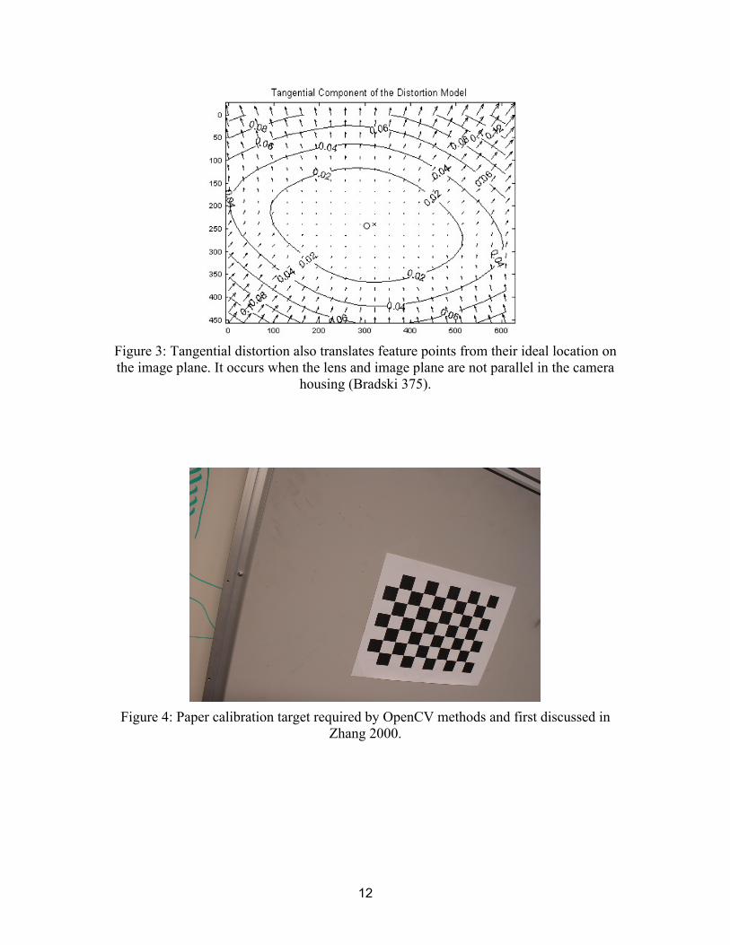
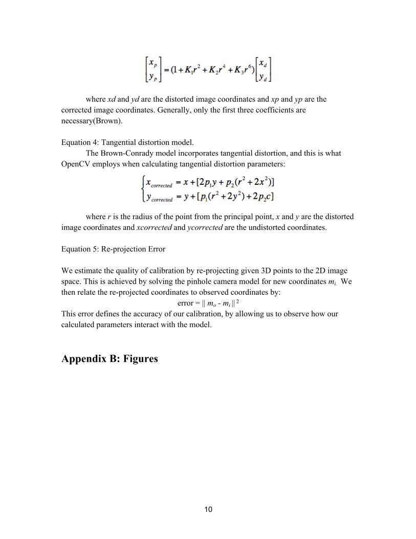
Figure 3: Tangential distortion also translates feature points from their ideal location on the image plane. It occurs when the lens and image plane are not parallel in the camera

housing (Bradski 375).

Figure 4: Paper calibration target required by OpenCV methods and first discussed in Zhang 2000.

12

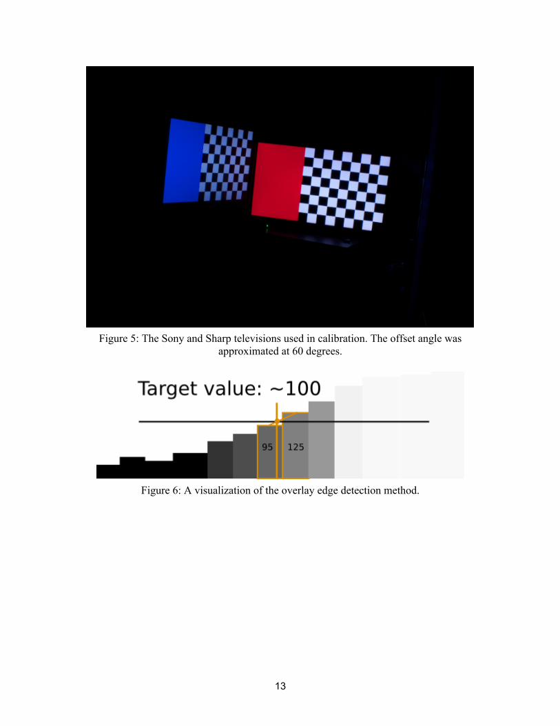
Figure 5: The Sony and Sharp televisions used in calibration. The offset angle was approximated at 60 degrees.

Figure 6: A visualization of the overlay edge detection method.

13

Figure 7: The first method of edge detection. We fit lines to edges calculated along the entire length of the checkerboard (green). Each line is then located with respect to the

initial guesses (red). The final intersections are calculated and return (orange).

Figure 8: The four corner edge detection method. We build each guess using line segments, which fit to the squares of the checkerboard.

14

References "BBC News - Driverless Car: Google Awarded US Patent for Technology." BBC - Homepage. Web. 28 Jan. 2012. <http://www.bbc.co.uk/news/technology-16197664>. Bradski, G. and A Kaehler. 2008. Learning OpenCV. O’Reilly Media, Inc., Sebastopol, CA. Brown, D. C. 1971. Close-Range Camera Calibration. Photogrammetric Engineering 37(8):855-866.

Duraiswami, Ramani. "Lecture 9: Camera Calibration." Ramani Duraiswami Personal Page. University of Maryland Institute for Advanced Computer Studies, 5 Oct. 2000. Web. 7 Jan. 2012. <www.umiacs.umd.edu/~ramani/cmsc828d/lecture9.pdf>.

Weng, J., Cohen, P. and M. Herniou. 1992. Camera Calibration with Distortion Models and Accuracy Evaluation. IEEE Transactions on Pattern Analysis and Machine Intelligence, Vol. 14, No. 10, October. Zhang, Z. 2002. A Flexible New Technique for Camera Calibration. Technical Report MSR-TR-98-71, Microsoft Research, Redmond, WA.

15