The macroevolutionary dynamics of

adaptive landscapesJosef C UyedaPostdoctoral fellow

iBEST & Dept of BiologyUniversity of Idaho

Reductionism & the Modern Synthesis

“Change in allele frequency over time”

Wright

Dobzhansky

Stebbins Fisher

Simpson

Haldane

Microevolution

Macroevolution

Microevolutionary patternsWe now know that we can study evolution in real time

16.06 g(1976)

17.13 g(1978)

Average weight

Response to selection

6.66% change in body size in 1 generation

(2 years)Conservatively, let’s assume that only a fraction is due to

evolution:i.e. 1% change in body size in

1 generationGrant and Grant, 2002

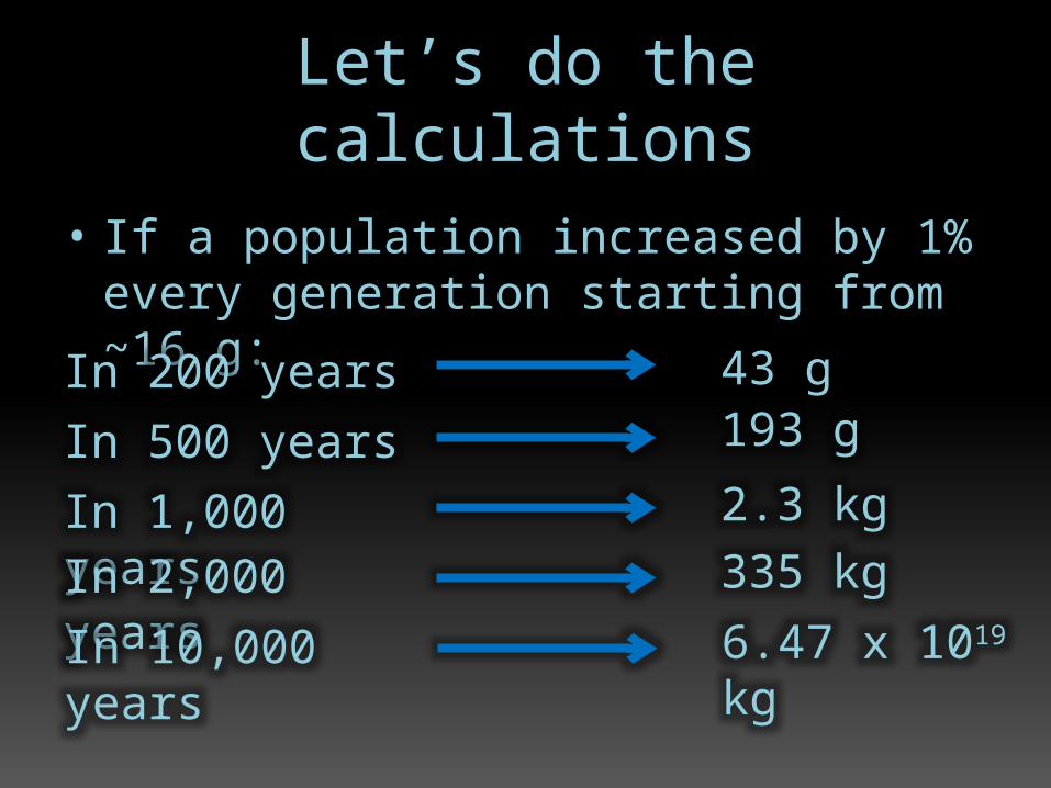
Let’s do the calculations

• If a population increased by 1% every generation starting from ~16 g:In 200 years

In 500 years

In 1,000 yearsIn 2,000 years

43 g193 g

2.3 kg335 kg

In 10,000 years

6.47 x 1019 kg

Thousands of years

Thousands of years

Thousands of years

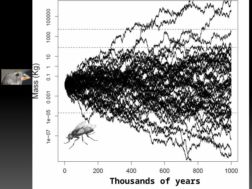
The Paradox of Stasis (Hansen & Houle 2004):Organisms seem to be able to evolve far more than they do over macroevolutionary scales

Empirical studies often find:• Strong (and often persistent) directional selection

(Hereford et al. 2004, Morrissey & Hadfield 2012)

• High levels of additive genetic variance (Mousseau & Roff 1987, Houle 1992)

• Rapid evolutionary rates(Hendry & Kinnison 1999, Kinnison & Hendry 2002)

…yet stasis in the fossil record (Gingerich 1983, 2002)

…and BM in comparative data?

How do we reconcile patterns at different scales?

All studies of phenotypic evolution measure comparable

quantities

How can we see the pattern across scales of time?

We measure two quantities:

(1) “time for evolution”(2) Δ mean body size

Pop Bmean(z)

Pop Amean(z)

Time interval

Pop X

Pop Bmean(z)

Pop Amean(z)

Time interval

Phenotypic divergence database (Uyeda, Hansen, Arnold & Pienaar, 2011. PNAS.)

Only animals, mostly

vertebrates, but also some inverts

Only traits related to linear body size

change

Field, Fossil and Phylogenetic

comparative data

>8000 data points from> 150 studies

Intervals from < 1 yr to 360 my

Thousands of years

Microevolutionary dataFossil dataPhylogenetic comparative data

Uyeda et al., PNAS, 2011

2 years

Microevolutionary dataFossil dataPhylogenetic comparative data

Uyeda et al., PNAS, 2011

800,000 years

Microevolutionary dataFossil dataPhylogenetic comparative data

Uyeda et al., PNAS, 2011

332.4 myMRCA of all mammals

Microevolutionary dataFossil dataPhylogenetic comparative data

Uyeda et al., PNAS, 2011

Average size change for all monotremes vs. all other mammals

Microevolutionary dataFossil dataPhylogenetic comparative data

Uyeda et al., PNAS, 2011

Microevolutionary dataFossil dataPhylogenetic comparative data

Uyeda et al., PNAS, 2011

Microevolutionary dataFossil dataPhylogenetic comparative data

Uyeda et al., PNAS, 2011

Microevolutionary dataFossil dataPhylogenetic comparative data

Uyeda et al., PNAS, 2011

Simpson’s Adaptive Zones

Model fits:Brownian Motion (BM)Multiple-burst (MB) – Poisson Point Process

MB model fits:

Dataset Parameter Estimates

Stasis SD Burst SD Ave. burst time

Whole dataset 𝜎ො��𝑝 = 0.096 𝜎ො��𝑘 = 0.27 25.0 my

Microevolutionary & Fossil 𝜎ො��𝑝 = 0.087 𝜎ො��𝑘 = 0.25 1.5 my

Phylogenetic 𝜎ො��𝑝 = 0.086 𝜎ො��𝑘 = 0.22 21.8 my

AIC = -9142.5 AIC = -9018.0 AIC = -7878.0

Time

Ph

en

oty

pe

Million-year waiting times

“Ephemeral” divergence over short timescales(Futuyma 1987)

Time

Ph

en

oty

pe

Adaptive peak shifts, stabilizing selection & genetic drift

Adaptive Zones/Niches

θ1 θ2 θ3

α

σ2

ln2/α = Phylogenetic Half-Life

Compare models(e.g. by AIC)

The “best” model may still be bad

OU models are not always well-behaved statistically

Problems:

OU models are valuable because of their biological

realism

…but where did the biology go?

Bayesian Reversible-Jump OU Modeling

FlexibleCan infer adaptive shifts and compare to a

priori hypotheses

Can incorporate additional data/realism through informative priors

Customize to test specific hypotheses

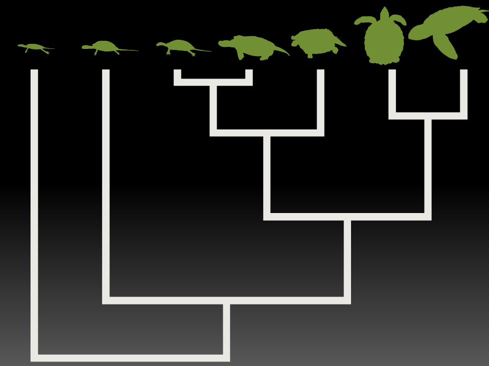
Turtles and Tortoises (Jaffe et al. 2011)

(Uyeda and

Harmon, 2014)

Habitat Modelbayou Model

2 ln BF = 15.24

surface

(Ingram &

Mahler, 2012)

bayou : 8 – 167 cm surface : 2.9x10-170fm– 1.96x1044 km surface:

92.6my

(Uyeda and

Harmon, submitt

ed)

habitatbayou

Habitat Modelbayou Modelsurface Modelbayou Model

𝝈  𝟐 Optima Phylogenetic half-life (my)

prior

We can generate better hypotheses

Jaffe et al. (2011) Marine, Freshwater, Terrestrial and

Island

Only Marine was found by bayou.

Better hypothesis? Aquatic life history + high

environmental temperature

But is it stabilizing selection or adaptive zone shifts or….?

• 85 taxa• Body size (SVL)• Use 3 different

priors:• Weakly

informative (Free)• Blunderbuss

model (Stasis shifts)

• Quantitative genetic model (Peak shifts)

Anolis

Parameterize with the “Blunderbuss”

σ2/(2α)

ln2/α

Quantitative Genetics Model(Lande 1976)

𝑑𝑍 𝑡=−α (𝑍 𝑡−1−θ )𝑑𝑡+σ 𝑑𝑊𝑡

Stabilizing Selection

Genetic Driftα = h2VP/(VP+ω2) σ2 = h2VP/Ne

QG model priors

h2=estimated in anoles to be ~0.55 for body size

VP=estimated from the data

Ne = 99% CI between 1000 and 400,000 (mean 22,000)

ω2= Stabilizing & directional selection gradients estimated from wild populations

QG Model Posteriors

Posterior

Prior

Parameterization Marginal lnL 2 ln BF: Free vs. _____

Free -16.4 0

Blunderbuss -24.9 17.0Lande (QG) -37.7 21.3

Both Blunderbuss and Lande models perform much more poorly than free parameterization

Can also combine these interpretations with ecotype-based hypotheses…..

Regimes Parameterization Convergence Marginal lnLFixed- Ecotype Free Yes 9.83Fixed- Ecotype Blunderbuss Yes 2.73Fixed- Ecotype Free No -3.62Fixed- Ecotype Lande (QG) Yes -6.70Fixed- Ecotype Blunderbuss No -14.16Free Free No -16.41Fixed- Ecotype Lande (QG) No -18.66Free Blunderbuss No -24.93Free Lande (QG) No -37.73

Convergent, Ecotype-based regimes fit tree best, but should not be interpreted as either Blunderbuss or Lande model

Time

Ph

en

oty

pe

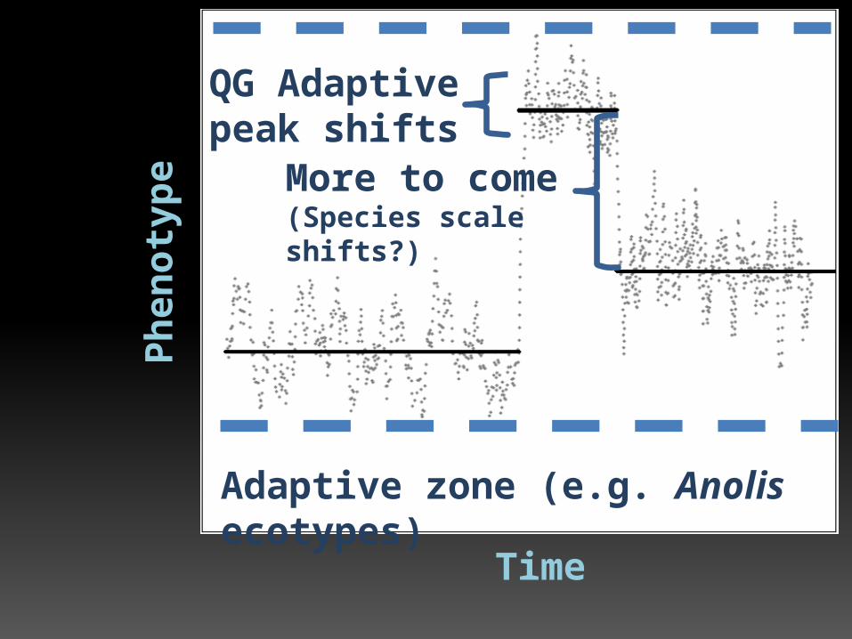
Adaptive zone (e.g. Anolis ecotypes)

QG Adaptive peak shifts

More to come(Species scale shifts?)

A broader framework: Combining fossils, microevolution and

phylogenetic comparative data

Fossil timeseries

Microevolutionary timeseries

Quantitative genetic & selection parameters

Goal: Powerful, customizable phylogenetic comparative methods for testing user-specific biological hypotheses

http://www.arborworkflows.com/

AcknowledgementsFunding and Support

National Science FoundationResearch Council of NorwayBEACON CenteriBEST, U. of IdahoOSU Zoology departmentCEES, U. of Oslo, Norway

Other assistance Phil Gingerich

Andrew HendryLynne HouckPaul JoyceJoe Felsenstein

Coauthors and collaborators

Thomas HansenJon EastmanLuke HarmonStevan J ArnoldJason PienaarMatt Pennell

Aaron ListonMike BlouinDavid LytleHarmon LabHansen LabArnold Lab