Reducing Run-Time Adaptation Space via Analysis of PossibleUtility Bounds

Clay StevensUniversity of Nebraska-Lincoln

Department of Computer Science and Engineeringclay.stevens@huskers.unl.edu

Hamid BagheriUniversity of Nebraska-Lincoln

Department of Computer Science and Engineeringbagheri@unl.edu

ABSTRACT

Self-adaptive systems often employ dynamic programming or sim-ilar techniques to select optimal adaptations at run-time. Thesetechniques suffer from the “curse of dimensionality", increasing thecost of run-time adaptation decisions. We propose a novel approachthat improves upon the state-of-the-art proactive self-adaptationtechniques to reduce the number of possible adaptations that needbe considered for each run-time adaptation decision. The approach,realized in a tool called Thallium, employs a combination of auto-mated formal modeling techniques to (i) analyze a structural modelof the system showing which configurations are reachable fromother configurations and (ii) compute the utility that can be gen-erated by the optimal adaptation over a bounded horizon in boththe best- and worst-case scenarios. It then constructs triangularpossibility values using those optimized bounds to automaticallycompare adjacent adaptations for each configuration, keeping onlythe alternatives with the best range of potential results. The ex-perimental results corroborate Thallium’s ability to significantlyreduce the number of states that need to be considered with eachadaptation decision, freeing up vital resources at run-time.

KEYWORDS

formal methods; self-adaptive systems; run-time adaptation; multi-objective optimizationACM Reference Format:

Clay Stevens and Hamid Bagheri. 2020. Reducing Run-Time AdaptationSpace via Analysis of Possible Utility Bounds. In 42nd International Confer-

ence on Software Engineering (ICSE ’20), May 23–29, 2020, Seoul, Republic of

Korea. ACM, New York, NY, USA, 13 pages. https://doi.org/10.1145/3377811.3380365

1 INTRODUCTION

Self-adaptive systems are becoming more pervasive, particularlyin applications such as autonomous vehicles and medical or IoTdevices [19, 24, 36, 57]. These systems need to quickly adapt toan uncertain, dynamic environment without external intervention,which is especially challenging given the nearly infinite situationssuch environments may present, the short window of time available

Permission to make digital or hard copies of all or part of this work for personal orclassroom use is granted without fee provided that copies are not made or distributedfor profit or commercial advantage and that copies bear this notice and the full citationon the first page. Copyrights for components of this work owned by others than theauthor(s) must be honored. Abstracting with credit is permitted. To copy otherwise, orrepublish, to post on servers or to redistribute to lists, requires prior specific permissionand/or a fee. Request permissions from permissions@acm.org.ICSE ’20, May 23–29, 2020, Seoul, Republic of Korea

© 2020 Copyright held by the owner/author(s). Publication rights licensed to ACM.ACM ISBN 978-1-4503-7121-6/20/05. . . $15.00https://doi.org/10.1145/3377811.3380365

to adapt, and the potentially limited computing resources availablefor making adaptation decisions at run-time.

In an ideal scenario where adaptations are instantaneous andimmediately beneficial, a reactive self-adaptive system can respondeffectively after a change in the environment has been detected.However, in cases such as provisioning a new cloud-based virtualmachine [40], the adaptations enacted by the system may takesome time, requiring a proactive approach which can account forthe latency of adaptation tactics [51]. While such proactive, latency-aware (PLA) approaches promise to improve the overall fitness ofthe adaptations chosen [15, 45], they need to look ahead and predictfuture states of the environment. Recent approaches to PLA self-adaptive systems model the environment as a stochastic processindependent of the state of the system [45]. Adaptation decisionscan then be made via stochastic planning using the predictions offuture states of the environment as input.

Historically, stochastic planning problems have been describedand modeled using Markov decision processes (MDPs) [53], whichcan be solved using dynamic programming to optimize some utilityor cost. If the number of distinct properties or settings available tothe system to adapt is large, this solution can suffer from Bellman’scurse of dimensionality [11], where the number of states that mustbe visited and evaluated grows factorially based on the number ofvalues that can be assumed by the variables representing the systemstate. Prior decision theoretic planning research has explored waysto curtail this state explosion, such as minimization of MDPs [31, 46],reachability analysis [12], and machine learning [25, 54].

However, despite significant progress, the adaptation space—thepossible state transitions that must be pondered for each run-timeadaptation decision—is still enormous, even considering only allow-able adaptations. This, in turn, renders dynamic run-time adaptationfor real-world systems expensive in practice. This is especially prob-lematic in volatile environments like distributed pervasive systems,where high volumes of routinely volatile software componentsoften exist and coordinate in tandem. There is, thus, a need formethods to facilitate efficient analysis of huge adaptation spaces.

In this paper, we present a novel approach, dubbed Thallium1,that automatically trims the adaptation space to be explored at run-time by the underlying adaptation decision maker. Unlike all priortechniques, Thallium retains only the adaptations with (Pareto-) optimal potential to provide the best utility. Thallium recog-nizes opportunities for trimming the dynamic adaptation space bycombining the state-of-the-art structural and behavioral modeling

1Thallium (Tl, atomic number 81) is a metallic element with very few strong lines inits emission spectrum; the light produced by burning it is trimmed to only a few bandswhen passed through a prism.

ICSE ’20, May 23–29, 2020, Seoul, Republic of Korea Clay Stevens and Hamid Bagheri

techniques [16, 46] for reachability analysis with a possibilistic pro-cess [27] for bound analysis of the utility achievable from eachsystem state.

Specifically, using lightweight model checking, Thallium ana-lyzes the structural system model to produce a Markov decisionprocess capturing the possible adaptations from each system state.It then employs probabilistic model checking to derive informationfrom the behavioral system model about the bounds on the util-ity achievable from each state. Thallium then utilizes possibilisticanalysis to resolve values representing the potential of each systemstate with respect to each optimization objective, accounting forboth the positive and negative consequences of uncertainty in theenvironment. Such automatically derived information is used inconcert with the reachability information to spot the Pareto-frontierin terms of potential for the valid adaptions from each state. Prun-ing away non-optimal or strictly dominated adaptations resultsin a trimmed MDP that only includes the adaptations that lead tostates with the Pareto-optimal potential, which in turn drasticallyreduces the analysis time for each dynamic adaptation decision. Tosummarize, this paper contributes:

• Effective adaptation space reduction at run-time.We introducea novel approach for effective trimming of the adaptationspace to be analyzed for each run-time adaptation decision,achieving remarkable speed-ups in dynamic adaptation. Thenovelty of our approach comes in using a possibilistic analy-sis to combine prior approaches in reachability analysis withan analysis of the best- and worst-case bounds on adapata-tion utility.

• Implementation: We have realized the ideas in Thallium,a framework which relies on the Alloy lightweight model-checker [34] to generate an MDP representing the allowableadaptations of the system and on the PRISM-Games exten-sion of the PRISM Model Checker [17, 37] to perform thebound analysis. We make Thallium publicly available to theresearch and education community [60].

• Experimental evaluation: We present results from experi-ments run on diverse subject systems—rigorously replicatingprominent earlier studies—corroborating Thallium’s abil-ity to significantly reduce the effort required for run-timeadaptation without sacrificing overall system utility.

In the remainder of this paper, we describe the motivation andintuition behind our approach in Section 2, followed by a detailedexplanation of our approach in Section 3. Sections 4 and 5 coverour experiments and their results, and Section 6 discusses possiblethreats to validity. Sections 7 and 8 conclude with an overview ofrelated work followed by a summary of our contributions.

2 ILLUSTRATIVE EXAMPLE

In this section, we describe the motivation and underlying insightof our research by way of an illustrative example. We consider apublish-subscribe messaging system used to monitor audio datacollected from various sources, where each received chunk of datamust be streamed to (and acknowledged by) an arbitrary number ofsubscribers. Audio data is collected from each source by a dedicatedpublisher service, which streams the data to a relay service for

Source Source

Publisher

Subscriber

Relay

Source

Publisher Publisher

Subscriber Subscriber

Relay

Figure 1: Pub-sub system example

distribution to the subscribers. An overview of the relationships ofthe various parts of the system is shown in Figure 1.

Each publisher can only harvest from one source, and can onlysend data to a single relay. Each relay can only sustain a limitednumber of total connections (or load) comprising publishers, sub-scribers, and “downstream” relays, beyond which the latency ofpacket delivery through that relay increases sharply. The goal ofthe system is to deliver the streamed audio to each subscriber withas low a latency as possible, with steep penalties associated withaudio latencies above a certain threshold. The system adapts tochanges in its environment in the following ways:

• PUB+: As needed, the system can provision a new publisherservice to harvest the audio from a new or otherwise un-harvested source, or assign that source to a running but idlepublisher. There is a cost for each online source that is notbeing harvested, and a cost associated with each runningpublisher. Provisioning a new publisher takes a non-zeroamount of time before the publisher starts harvesting audiofrom a source, adding a tactic latency (Lp ) to this adaptation.

• RLY+: As needed, the system can provision a new relayservice for use in future connections. Each running relay ser-vice carries an attended cost for the duration of its operation,whether it is serving any connections or not. There is alsosome tactic latency (Lr ) involved in provisioning a new relay.Each relay also has a threshold number of active connections,below which the relay is able to immediately handle dataon that connection, and above which all connections to thatrelay begin to suffer additional latency (as the relay beginsto buffer and switch between connections).

• PUB-, RLY-: As needed, the system can also deactivate apublisher or a relay (or both). No tactic latency is assumedhere.

• WAIT: For the sake of completeness and to represent thepassage of time in the case of tactics with latency, the systemcan elect to do nothing and simply wait for the next time step.

Figure 2 shows an example MDP that represents this system. Inthis Markov decision process, the states are labeled using a four-valued tuple consisting of the number of publishers, the number ofrelays, the number of time steps remaining for a PUB+ tactic, andthe number of time steps remaining for a RLY+ tactic, respectively.

Reducing Run-Time Adaptation Space via Analysis of Possible Utility Bounds ICSE ’20, May 23–29, 2020, Seoul, Republic of Korea

Figure 2: System MDP example (1-2 publishers/relays, la-

tency = 1) considering reachability only. Each adaptation de-

cision must evaluate on the order of 4 adaptations.

The number of publishers and of relays are both constrained to beeither one or two, and Lp = Lr = 1.

The adaptation goal in the system is tominimize the total cost ofthe system over time, which can be computed for each time step as afunction of the state of the system and the state of the environmentat that time. The system state s at time t can be modeled as a tuple:

• P(st ): the number of active/ready publishers,• P ′(st ): the number of provisioned publishers (including thosestill starting up but not yet active/ready),

• R(st ): the number of active relays, and• R′(st ): the number of provisioned relays.

The environment state e at time t can be modeled as a pair:• Q(et ): the number of active sources, and• S(et ): the number of active subscribers.

At each time step, the overall cost for that step comprises fourobjectives that each map the system and environment states at thattime to a real value, where S is the set of all system states and E isthe set of all environment states:

• The audio latency cost, CL : Q × N → R, a function of thecurrent average load on each active relay (λ : S × E → Q)and the connection threshold of the relays (T ∈ N), where

λ(st , et ) =S(et ) + P(st )

R(st )+ (R(st ) − 1),

• The publisher cost, Cp : N → R, which is a function of thenumber of provisioned publishers, P ′(st ),

• The relay cost, Cr : N → R, which is a function of thenumber of provisioned relays, R′(st ), and

• The unharvested source cost, Cs : N × N → R, which is afunction of the number of active publishers, P(st ), and thenumber of active sources, Q(et ).

To make the adaptation decision, a dynamic programming so-lution would need to recursively evaluate the total cost that couldbe produced by starting from each relevant system configurationup to some finite look-ahead horizon, H , and select the adaptationsleading to the state with the optimal result. H becomes yet anothermultiplier on the amount of work needed. The (potentially nearlyinfinite) values from the environment are additional multipliers,

Figure 3: Trimmed MDP produced using Thallium

(T = 1000, S(et ) ∈ {0..50},Q(et ) ∈ {0..10}). Adding a new relay

is not Pareto-optimal given the bounds of the environment

states, and can be disregarded.

drastically increasing the number of possible adaptations. To extendour pubsub example, consider such a system where P(st ) ∈ 1, 2,R(st ) ∈ 1, 2, and Lp = Lr = 1. The configuration space allows for16 unique configurations. If there will be at most 50 subscribers(S(st ) ∈ 0..50) and at most 10 active audio sources (Q(st ) ∈ 0..10)the space for the system and the environment would have 8,976members. If H = 5—quite small—a dynamic programming solutionmust still find optimal adaptations among 44,880 states.

State-of-the-art systems, such as PLA-SDP [45, 46], exploit theinsight that only a subset of states are reachable via adaptation fromany given state at a given time. Some adaptations–such as addingand removing a publisher–may be mutually exclusive. Others–suchas adding a relay or publisher–may take a non-trivial amount oftime to complete. To utilize the additional reachability information,PLA-SDP uses lightweight model checking to exhaustively explorethe structural relationships between states and construct a Markovdecision process (MDP) representing the allowable adaptationswithin the system. In our example, it would produce an MDP likethe one shown in Figure 2. This reduces the number of adaptationsthat need to be considered at each step within the horizon down to4 or fewer, depending on the current state.

However, PLA-SDP may still recursively consider adaptationsthat would not improve the overall outcome. If each relay in thesystem can simultaneously manage 1000 connections (i.e., the relayconnection threshold T = 1000), a single relay could easily handleall 50 subscribers and all 10 audio sources. Adding a second relaywould only increase the cost for the number of active relays, Cr ,without reducing the latency costCL . Given that the tactic of addinga new relay would still be reachable, it would still be considered byPLA-SDP for each step within the horizon, even though there wouldbe no benefit to selecting such a strategy under any circumstances.

Thallium aims to reduce the number of sub-optimal adaptationsconsidered by employing information about the bounds of thepossible values for each objective. In the example provided above,we would consider the best-case to be when there are no activesubscribers or sources and the worst-case to be when there are 50active subscribers and 10 active sources. In either case, adding a newrelay would only increase Cr without improving the cost for anyother objective (i.e., it would not be Pareto optimal), so Thalliumwould remove those adaptations from the consideration set. Withour assumed values, the MDP produced by Thallium would trimall states with more than one relay, greatly reducing the adaptationspace. The final MDP for our example is shown in Figure 3.

ICSE ’20, May 23–29, 2020, Seoul, Republic of Korea Clay Stevens and Hamid Bagheri

Figure 4: Thallium Overview

3 APPROACH

This section presents our approach to effectively trim the adaptationspace at run-time. As depicted in Figure 4, Thallium comprises fourautomated components. (1) The Reachability Analysis componentperforms lightweight model checking of a provided system struc-tural model to construct an intermediate Markov decision process(MDP) representing the states reachable via adaptation from eachsystem configuration. (2) The Utility Bounds Analysis componentleverages probabilistic model checking to analyze the behavioralsystem specification formalized as a stochastic multiplayer game(SMG). This step automatically determines new, previously unused,information about guaranteed bounds of achievable utility in thebest- and worst-case scenarios, which is, in turn, used to define afuzzy set [68] of possible utility values for each optimization objec-tive at each state. (3) The Potential Synthesis component leveragespossibilistic analysis [27, 67] to transform the derived fuzzy sets intoa single value representing the potential of each state to provide thehighest utility for each objective. Finally, (4) the MDP Optimization

component compares the available adaptations at each node in thederived MDP apropos their potential for each objective and prunesstrictly dominated adaptations from the final MDP.

Thallium requires the user to specify two formal models ofthe system: a structural model defining the states the system canassume and the transitions between them; and a behavioral model

specifying the behavior of the system as an SMG, including theprobabilities of each transition for players representing the systemand its operating environment. In this paper, we present examples ofthe structural models using Alloy [34], which allows users to modelsystems using a lightweight, approachable syntax familiar to manydevelopers. We present the behavioral models as SMGs definedusing the PRISM [37] model checker, as it has been widely usedin research [1, 13, 22, 23] and has extensive documentation [52].These widely-used, familiar modeling techniques ease the burdenplaced on users to develop the models required for input.

3.1 Reachability Analysis

To construct an intermediate MDP representation of the system,Thallium generates the graph of all “reachable” states in the systemusing the method described by Moreno, et al. [46]. Reachability isdefined using the following predicates for system states c, c ′ ∈ C:

• Immediate Transitions RI (c0, c1) — c1 can be reached from c0using an immediate transition (i.e., applying no tactic or onewith no latency);

• Delayed Transitions RD (c0, c1) — c1 can be reached from c0in one time interval using a delayed transition by applyinga tactic with latency; and

• Transitive Transitions RT (c0, cn ) — cn can be reached in onetime interval using a delayed transition followed by one ormore immediate transitions, or more formally:

∃ c1, ..., cn−1 : RD (c0, c1) ∧ RI (c1, c2) ∧ ... ∧ RI (cn−1, cn )

These predicates can be used to fully define the feasible transitionmatrix of the system configuration MDP, which requires evaluatinga large number of possible combinations of tactics/transitions. Togenerate such a transition matrix, we use Alloy [34] to formallyspecify both the system configuration and the reachability predi-cates. Alloy is a formal modeling language based on relational logic,amenable to fully automated yet bounded analysis. It facilitates rep-resenting abstract system structures and the relationships betweenthem as a set of constraints. Once a system has been described as acollection of structural type signatures and constraints, the AlloyAnalyzer can be used to automatically find model instances thatsatisfy all the constraints.

Three Alloy specifications are conjoined to define the structuralsystem configuration model: (1) the system state specification, (2)the tactics specification that can execute transitions between states,and (3) a trace specification that maps a configuration state to aset of other configuration states that can be reached by sequentialapplications of allowed tactics. Figure 5 partially represents thesystem state specification for our running example (cf. Section 2).According to lines 19–23, the SystemCfg signature contains twofields, activeRlys and activePubs, that represent the number ofactive relays and publishers, respectively; the prog field representsthe latency of any delayed tactics as a unique progress value foreach tactic with latency.

The next step is to formalize the progress on each particular tac-tic, which captures whether the tactic will reach a state succeedingthe current state in the model’s ordering. Such formal specificationof each tactic’s progress enables us to automatically compute RD .Each tactic will need a predicate definition to check whether thesuccessor thereof can be reached in a single time interval and tomodel the effect of the tactic completion. As a concrete example,Figure 6 represents the AddRly_Prog tactic progress specification.This predicate holds between two states for transitions involvingthe AddRly tactic with latency.

Given a concrete analysis scope that bounds the search for eachtop-level signature in the system specification, e.g., SystemCfg andProg, Thallium uses the Alloy analysis engine to exhaustivelygenerate all model instances that satisfy the RD predicate. Thoseinstances are then encoded in a lookup table for use at run-time.

Computing RI is conducted by automatically generating tracesrepresenting the sequential applications of each no-latency tacticthat can be applied to transitions from one state to another. Figure 7represents the trace signature definition alongwith its predicates forthe AddRly no-latency tactic. According to lines 4–6, the TE tracesignature contains two fields–config and start_tactics–thatrepresent a particular system configuration and the set of tacticsneeded to be started to reach that state from the preceding statein the trace, respectively. Tactic-specific predicates formalize both

Reducing Run-Time Adaptation Space via Analysis of Possible Utility Bounds ICSE ’20, May 23–29, 2020, Seoul, Republic of Korea

1 sig RlyCount {} // each value in the system state needs a2 sig PubCount {} // signature to represent its domain34 abstract sig Tactic {} // tactics5 abstract sig LTactic // tactics w/ latency6 extends Tactic {}78 // define all tactics with latency9 one sig AddRly , AddPub extends LTactic {}10 // define all instantaneous tactics11 one sig DropRly , DropPub extends Tactic {}1213 // each tactic with latency requires a progress value14 abstract sig Prog {}15 sig AddRly_P extends Prog {}16 sig AddPub_P extends Prog {}1718 // the system configuration itself19 sig SystemCfg {20 activeRlys : one RlyCount ,21 activePubs : one PubCount ,22 prog : LTactic -> Prog23 } {24 // every tactic in LTactic has a progress ...25 prog.univ = LTactic26 // ...at most one...27 ~prog.prog in iden28 // ...and each from its own domain.29 prog[AddRly] in AddRly_P30 prog[AddPub] in AddPub_P31 }

Figure 5: System state specification for the pub-sub exam-

ple (cf. Section 2), including instantaneous tactics (DropRly,DropPub) and tactics with latency (AddRly, AddPub). Latency is

modeled by adding a progress field to the configuration for

each tactic with latency.

1 open util/ordering[RlyCount] as RlyCount_O2 open util/ordering[AddRly_P] as AddRly_PO34 pred AddRly_Prog[c,c' : SystemConfig] {5 (c.prog[AddRly] , AddRly_PO/last) implies {6 // if the tactic is running , the predicate holds for7 // successor states that have the next progress value8 c'.prog[AddRly] = AddRly_PO/next[c.prog[AddRly ]]9 c'.prog[AddRly] = AddRly_PO/last implies {10 // if that is the last progress value , then11 // it holds if the relevant state value has been12 // updated to reflect the tactic 's execution13 c'. activeRlys = RlyCount_O/next[c.activeRlys]14 } else {15 // otherwise , the state value stays the same16 c'. activeRlys = c.activeRlys }17 } else {18 // if the tactic is not running , assert that it19 // stays the same in the successor20 c'.prog[AddRly] = AddRly_PO/last21 c'. activeRlys = c.activeRlys }}22 // the progress predicates can be composed sequentially23 // to compute the actual delayed reachability predicate24 pred RD[c,c' : SystemConfig] {25 some tc : SystemConfig |26 AddRly_Prog[c, tc] and AddPub_Prog[tc, c'] }

Figure 6: Tactic progress predicate for the pubsub example.

This predicate holds between two states for transitions in-

volving a tactic (AddRly) with latency.

whether a particular tactic can be applied to the current system con-figuration (lines 9–13) and the results of applying an instantaneousconfiguration if applicable (lines 15–24). The traces fact (lines25–32) specifies which transitions from one system configurationto another are valid by composing the applications of the various

1 open util/ordering[TE] as trace23 // Trace of sequential applications of no-latency tactics4 sig TE {5 config : one SystemCfg6 start_tactics : set T }7 // Checking whether the tactic can be applied to the8 // current system configuration9 pred AddRly_ok[e : TE] {10 // tactic not running11 e.config.prog[AddRly ]] = AddRly_PO/last12 !( AddRly in e.start_tactics)13 !( DropRly in e.start_tactics) }14 // Initiate the progress for the AddRly tactic15 pred AddRly_start[e, e' : TE] {16 AddRly_ok[e]17 e.config.activeRlys , RlyCount_O/last18 e'. start_tactics = e.start_tactics + AddRly19 let c = e.config , c' = e'. config | {20 // start the progress for this tactic ,21 // and change nothing else22 c'.prog[AddRly] = AddRly_PO/first23 equals[c, c']24 (LTactic - AddRly) < : c.prog in c'.prog }}25 fact traces {26 let fst = trace/first | fst.starts = none27 all e : TE - trace/last | let e' = next[e] | {28 equals[e, e'] and equals[e', trace/last]29 } or DropRly_enact[e, e']30 or DropPub_enact[e, e']31 or AddRly_start[e, e']32 or AddPub_start[e, e'] }

Figure 7: Example trace predicates to track pubsub system

evolution. The traces fact defines which transitions from

one configuration to another are valid by composing the ap-

plication of the tactic-specific predicates.

tactic-specific predicates, e.g., DropRly_enact and AddRly_start.Thallium again uses the Alloy analysis engine to obtain all validtraces (i.e., those satisfying the traces fact) and capture them in alookup table for RI to be used at run-time.

3.2 Utility Bounds Analysis

To compute the upper- and lower-bounds on the overall systemutility achievable from a given state, Thallium analyzes the inputbehavioral model as a stochastic multiplayer game (SMG), in whichplayers alternate selecting transitions based on the transitions’assigned probabilities. The SMG is analyzed using a probabilisticmodel checker [17] as described by Cámara, et al. [16].

The system configuration and its transitions modeled in theSMG, are controlled by one player, and the environment’s stateis controlled by another player. The players take turns selectingfrom the available transitions in the underlying model until thetime horizon, measured in discrete time steps, has been reached.Depending on the properties set on the execution of the game, theplayers can either cooperate to achieve a shared goal or competeby pursuing their own individual goals. In the context of PRISM-Games, these properties can be expressed using the rPATL logic [17],a branching time temporal logic based ultimately on ATL[2]. It hasbeen widely used for game-theoretic reasoning systems involvingmultiple agents, such as the system and environment in adaptationdecisions.

Our research uses both the coalition operator ⟨⟨C⟩⟩ adoptedfrom ATL and the reward operator ⟨⟨C⟩⟩Rrmax=?[F

∗ϕ], which is anextension of the generalized reward operator, R [28]. This operator

ICSE ’20, May 23–29, 2020, Seoul, Republic of Korea Clay Stevens and Hamid Bagheri

quantifies the maximum accumulated reward r that can be guaran-teed by the players in coalitionC along any paths leading to a statesatisfying ϕ, regardless of the actions taken by any players outsidethe coalition. We use PRISM-Games to verify two properties ofthe upper-bound for the cumulative reward and the lower-bound forthe cumulative reward for each reachable system configuration. Inthe following formulas, sys is the player representing the adaptivesystem, env is the player representing the stochastic environment,and ω is a predicate defining a termination state.

⟨⟨sys⟩⟩RUmax=?[Fcω] (1)

⟨⟨sys, env⟩⟩RUmax=?[Fcω] (2)

Property 1 (the lower-bound for the cumulative reward) representsthemaximumutilityU for the overall system, that can be guaranteedby sys alone along any path leading to a terminal state; this is theworst-case that can be achieved by an optimal player. Property 2(the upper-bound for the cumulative reward) represents the best-casefor the overall system utility, wherein sys and env are workingtogether to maximize the reward over time.

The PRISM-Games commences with a definition of both theplayers and the rewards, based on the relevant utility functions,followed by a series of modules for each set of independent, i.e.,not mutually-exclusive, tactics and the environment evolution. Theturns are controlled by a specific module for each turn, whichis synchronized with the tactic modules for that turn. The timeintervals and horizon are modeled using a special clock module thatkeeps track of the discrete time progression. Rewards are assignedduring a distinct reward turn by a corresponding module.

As a concrete example, Figure 8 shows a tactic module from thepubsub behavioral model of the pubsub system. Each tactic moduleincludes all possible outcomes for the MDP. For example, five possi-ble outcomes for the relay module tactic have been modeled in thefigure, where each one is labeled using the same transition label.This allows PRISM-Games to resolve each step in the simulationusing whichever of the concurrent tactics would provide the beststrategy for the coalition.

Similarly, each possible evolution of the environment’s statemust be provided as a possible choice of action for PRISM-Games,which we define in a module dedicated to that evolution. Figure 9shows an example environment evolution module. It represents thenumber of active subscribers in the pubsub system. A similar mod-ule would be synchronized using do_env to simulate the numberof audio sources in the pubsub environment.

We can then resolve the lower- and upper-bounds for the cu-mulative reward, as shown in Equation 1 and Equation 2, respec-tively. We vary the initial system state values (e.g., INIT_RELAYSand INIT_RPROG) for each tactic in order to determine the worst-and best-case utility that can be attained over the time horizon,starting from each admissible system configuration. The admissiblesystem configurations include configurations where the progresson a latency-bearing tactic is non-zero, indicating that the systemhad started, but not yet finished, executing a tactic.

Running the PRISM-Games models described above for eachexample computes a value for the properties defined in Equations 1and 2. We vary the constants used in the model to simulate startingfrom each possible system configuration. This produces a best-

1 module relay2 relays : [MIN_RELAYS .. MAX_RELAYS] init INIT_RELAYS;3 relay_prog : [MIN_RELAY_PROG .. MAX_RELAY_PROG] init INIT_RPROG;4 // skip; do nothing5 [do_sys] (turn=SYS_TURN) ->6 true;7 // initiate the latency -bearing tactic to inc. the value8 [do_sys] (turn=SYS_TURN) & (relays <MAX_RELAYS)9 & (relay_prog=MIN_RELAY_PROG) ->10 (relay_prog '= MAX_RELAY_PROG);11 // advance the progress for the latency -bearing tactic12 [do_sys] (turn=SYS_TURN)13 & (relay_prog >( MIN_RELAY_PROG +1)) ->14 (relay_prog '=( relay_prog -1));15 // finish the latency -bearing tactic16 [do_sys] (turn=SYS_TURN)17 & (relay_prog =( MIN_RELAY_PROG +1)) ->18 (relay_prog '= MIN_RELAY_PROG) & (relays '=( relays +1));19 // enact the no-latency tactic to decrement the value20 [do_sys] (turn=SYS_TURN) & (relays >MIN_RELAY_VAL)21 & (relay_prog=MIN_RELAY_PROG ->22 (relays '=(relays -1));23 endmodule

Figure 8: Example tacticmodule from the pubsub behavioral

model. The relay module has both an instantaneous tactic

(to drop a relay) and a tactic with latency (add a relay) and

must keep track of tactic progress.

1 module subscriber2 subscribers : [MIN_SUBS .. MAX_SUBS] init INIT_SUBS;3 [do_env] (turn=ENV_TURN) -> (subscribers '= MIN_SUBS);4 [do_env] (turn=ENV_TURN) -> (subscribers '=( MIN_SUBS +1));5 // ...6 [do_env] (turn=ENV_TURN) -> (subscribers '= MAX_SUBS);7 endmodule

Figure 9: Example environment evolutionmodule represent-

ing the number of active subscribers in the pubsub system.

and worst-case value for the cumulative utility achievable fromthat configuration. We can also compute the expected value usingPRISM by simulating the expected, probabilistic reward (using theR operator) with no coalition of players.

Those three values are interpreted to define a triangular distribu-tion of a fuzzy value, representing the membership of a utility valuein the set of possible utility values for the given reward. The worst-case value (U p ) represents the most-pessimistic result possible; noworse outcome is achievable so the degree of membership in theset of possible values is taken to be zero. Similarly, the best-casevalue (U o ) is assigned a degree of membership of zero, since it isthe most-optimistic value possible. The expected value (E(U )) isassigned a degree of membership of one; it is the most-likely value,and therefore should be a member of the set.

3.3 Potential Synthesis

The fuzzy values generated by computing the utility bounds arethen normalized and optimized to produce one value per rewardper state representing the “potential” of that state with respect tothat reward. The key insight in computing the potential state valueper reward, inspired by POISED [27], is to simultaneously optimizethree values from the possibility distribution by selecting a systemconfiguration. We define the optimization objectives as follows:

(1) Maximize the expected reward (or minimize the expectedcost), ze ≡ E(U ),

Reducing Run-Time Adaptation Space via Analysis of Possible Utility Bounds ICSE ’20, May 23–29, 2020, Seoul, Republic of Korea

Figure 10: Triangular possibility distribution with optimiza-

tion values (zp ,ze ,zo ) indicated. ze is the expected or most-

likely value, zp the “down-side”, and zo the “up-side”.

(2) Maximize the positive consequences of uncertainty or “up-side” potential, zo ≡ |U o − E(U )|, and

(3) Minimize the negative consequences of uncertainty or “down-side” potential, zp ≡ |U p − E(U )|.

Figure 10 depicts a schematic representation of the quantitiesinvolved in the calculation of the potential state value along witha triangular possibility distribution. In order to compare two ofthese fuzzy sets we must be able to resolve any trade-offs betweenthe values. For example, for one configuration, the value ofUo or“upside” may be greater than that of an alternate configuration(which is desirable), but the value of Up or “downside” may alsobe greater (which is not desirable). Also, the ranges for each of thethree objective values may differ, making direct comparison moredifficult. Therefore, we first normalize the values, and then reframethe overall problem as a single-objective optimization problem.

The values can be normalized by applying a linear normaliza-tion function, µzj , to map the domain of each of the three objec-tives zj (where j ∈ p, e,o) to a value between 0 and 1. A mappedvalue of 0 corresponds to the minimum value of zj and 1 corre-sponds to the maximum value, with a linear mapping of all inter-vening values [38]. With the values normalized, we reframe themulti-objective optimization problem as a single-objective opti-mization function via optimizing an auxiliary functionψ , returningthe weighted minimum of the normalized values, as shown in Equa-tion 3 withw j representing the weight :

argmaxc ∈C

ψ whereψ ≤ w j µzj and∑jw j = 1 for j ∈ {p, e,o} (3)

By maximizing the auxiliary function we also optimize the originalobjectives. Thallium stores the maximized value of ψ for eachsystem configuration as the potential metric for each configurationand uses it in the next step for trimming the MDP transitions.

3.4 MDP Optimization

With the potential values determined for each configuration andeach reward, Thallium can then compare adjacent transitions todetermine which transitions, if any, can be eliminated from thegenerated reachability graph (cf. Section 3.1).

Thallium compares each configuration by finding which of theneighboring transitions will move the system into a state whose po-tential is Pareto optimal with respect to all of the reward objectives,rather than using a single weighted composite value representing

Figure 11: Example potential values for pubsub system,

starting from (1,1,0,0). (1,1,0,1) and (1,1,1,1) are dominated

by the others for every objective, so the transitions to those

states (i.e., adding a relay) can be trimmed. (1,1,0,0) and

(1,1,1,0) form the Pareto frontier, as the former is better for

Cp and the latter for Cs while they are equal for CL and Cr .

all of the objectives. More formally, a transition t to a system con-figuration c will only be retained if there is no other transition t ′

to a different configuration c ′ such that the potential of any of therewards at c ′ is greater than the same reward potential at c and thepotential of all other rewards at c ′ is at least equal to the correspond-ing potential at c . All other transitions will be trimmed, leavingonly the Pareto-optimal siblings to be considered when selectingadaptations. An example using the pubsub system from Section 2is shown in Figure 11, which shows potential values from startingstate (1,1,0,0). The (1,1,0,1) and (1,1,1,1) states are dominated bythe others for every objective, so adaptations to those states (i.e.,adding a relay) can be trimmed. The (1,1,0,0) and (1,1,1,0) statesform the Pareto frontier, since the former is better for Cp and thelatter for Cs while they are equal for CL and Cr .

The resulting trimmed MDP produced by Thallium is thenused at run-time to facilitate efficient adaptation decision making,without sacrificing the overall system utility.

4 EVALUATION

Our evaluation of Thallium addresses these questions:• RQ1: How well does Thallium perform in reducing theadaptation space both offline and at run-time?

• RQ2: Does Thallium provide comparable utility for thesystem compared to the state-of-the-art approaches?

To answer these questions, we have designed and conductedexperiments using the apparatus we developed based on the pre-sented approach. Thallium uses the Alloy Analyzer [34] version4.2 to model the system configuration and generate the systemMDP, and the PRISM-Games [17] extension of the PRISM ModelChecker [37] version 4.3 to determine the utilities of the best, worst,and most-possible cases. We developed Thallium as a custom Javaprogram which generates possibility values and trims sub-optimaladaptations from the system configuration MDP.

4.1 Experimental Subjects

We used two exemplar systems—each from a separate domain—forour experiments: (1) SWIM [48], a simulator of self-adaptive webinfrastructure; and (2) DART [33, 43], a system that simulates ateam of unmanned aerial vehicles (UAVs) detecting targets whileavoiding threats during a reconnaissance mission. These systemsare described in more detail below.

ICSE ’20, May 23–29, 2020, Seoul, Republic of Korea Clay Stevens and Hamid Bagheri

SWIM: Our first experimental subject is SWIM (Simulator ofWeb Infrastructure and Management) [43], a self-adaptive systemdesigned to simulate a load-balanced web application. The systemsupports adding or removing servers as well as controlling a dimmersetting that regulates the level of content returned for each request.SWIM is implemented on top of OMNeT++, a discrete event simula-tion environment [63], and simulates only the high-level processingof web requests as computational work. The system is highly ex-tensible, providing monitoring information about the current stateof the simulation and effectors to simulate the execution of tactics.

We define SWIM’s system configuration, ci ∈ C , during an arbi-trary discrete time step, i , as the tuple (si ,di ,∆i ), where si repre-sents the number of active servers, di represents the setting of thedimmer—which increases or decreases the percentage of optionalcontent, with a corresponding decrease or increase to the servicerate, respectively—and ∆i represents the number of time steps re-maining for an active tactic execution. The environment state, ei ,for the same time step represents the number of web requests thatarrived at the server during that time step. The adaptation goals ofthe SWIM system are to (1) minimize the average response time,(2) minimize the server provisioning costs, and (3) maximize thepercentage of optional content delivered.

DART: As the second experimental subject, we use the DARTself-adaptive system developed by the CarnegieMellon Software En-gineering Institute [33, 47]. DART simulates a team of UAVs flyinga reconnaissance mission in formation over a bounded, hostile envi-ronment containing both reconnaissance targets and enemy threats.One of the drones is designated as the leader, and autonomouslydecides the actions the team should undertake in order to fulfillthe mission goals, such as changing altitude or formation. In ourexperimental scenario, the team flies along a planned route of Dequal segments at a constant rate, using a downward-facing sensorto detect as many targets as possible while avoiding destructionfrom any threats. Both the number and location of the targets andthreats are static, but unknown at the beginning of the run. Due tothat uncertainty, the team must self-adapt by changing altitude orformation to maximize the number of targets safely detected. Flyingat a lower altitude increases the probability of detecting a target, butalso increases the chance of being destroyed by a threat. Similarly,flying in a loose formation provides better target detection while atight formation decreases the probability of destruction.

4.2 Experimental Design

To address our research questions, we compared Thallium withthe state-of-the-art technique in proactive, latency-aware self adap-tation, namely PLA-SDP [46]. We conducted three experiments onour exemplar systems. For each, we applied both PLA-SDP andThallium to construct MDPs for the system. The MDP generatedby PLA-SDP for each system was considered a baseline for eachof the three experiments, against which we compared the relevantoutcomes using the trimmed MDPs produced by Thallium. Allthree experiments were run on a MacBook Pro with a 2.3 GHz IntelCore i5 processor and 16 GB of RAM.

Experiment 1. For the first experiment, we sought to evaluate Thal-lium’s effectiveness at reducing the size of the static adaptation

Figure 12: Percentage of adaptations trimmed by Thallium

from baseline (PLA-SDP) MDP for each evaluated system us-

ing different values for (wp ,we ,wo ) (see Section 3.3)

space represented by the system MDP. Both PLA-SDP and Thal-lium rely heavily upon the modeling choices and utility functionsspecified with the structural and behavioral models provided asinput, but Thallium also introduces additional configuration–theweights assigned to the optimization objectives during potentialsynthesis (see Section 3.3). As such, we used Thallium to generatemultiple MDPs for each system, with different weights for each. Wecompared the number of transitions in each of the those resultingMDPs to the number of transitions in the baseline MDP, reportingthe outcome as a percentage reduction compared to the baseline.

Experiments 2 and 3. For the second and third experiments, weexecuted simulators included with the SWIM and DART exemplars,respectively. We tested (1) the number of adaptations dynamicallyevaluated at run-time and (2) the overall system utility achievedwhen adapting based on the baseline MDP vs. a trimmed MDP gen-erated by Thallium. We varied the adaptation manager providedto guide adaptation–either the MDP from PLA-SDP or Thallium–and measured the number of adaptations evaluated during eachrun-time adaptation decision and the overall utility measurementrelevant to each exemplar. In addition, we introduced a purelyreactive adaptation manager to serve as a third comparison forExperiment 2, detailed in Section 4.4.

4.3 Experiment 1: Static MDP Trimming

For our first experiment, we evaluated Thallium’s effectiveness inreducing the size of the static adaptation space compared to PLA-SDP for each of our exemplar systems. As discussed in Section 3.3,the potential value generated for each system state and used forthe Pareto optimization is synthesized by normalizing and opti-mizing the three values from a triangular possibility distribution—zp , ze , zo—each with a corresponding weight. Since the weightingneeds to be specified by the user, we also sought to quantify theimpact of the weighting on the reduction of the adaptation space.Therefore, we ran Thallium on each exemplar system using eachof sixteen valid weight assignments, ranging from equal weightingto exclusively considering a single value. Figure 12 summarizes theresults for each system and each weighting, reporting the percent-age of allowable adaptations trimmed by Thallium compared tothe number in the MDP generated by PLA-SDP.

Reducing Run-Time Adaptation Space via Analysis of Possible Utility Bounds ICSE ’20, May 23–29, 2020, Seoul, Republic of Korea

(a) Num. adaptations evaluated for each adaptation decision

(b) Cumulative system utility

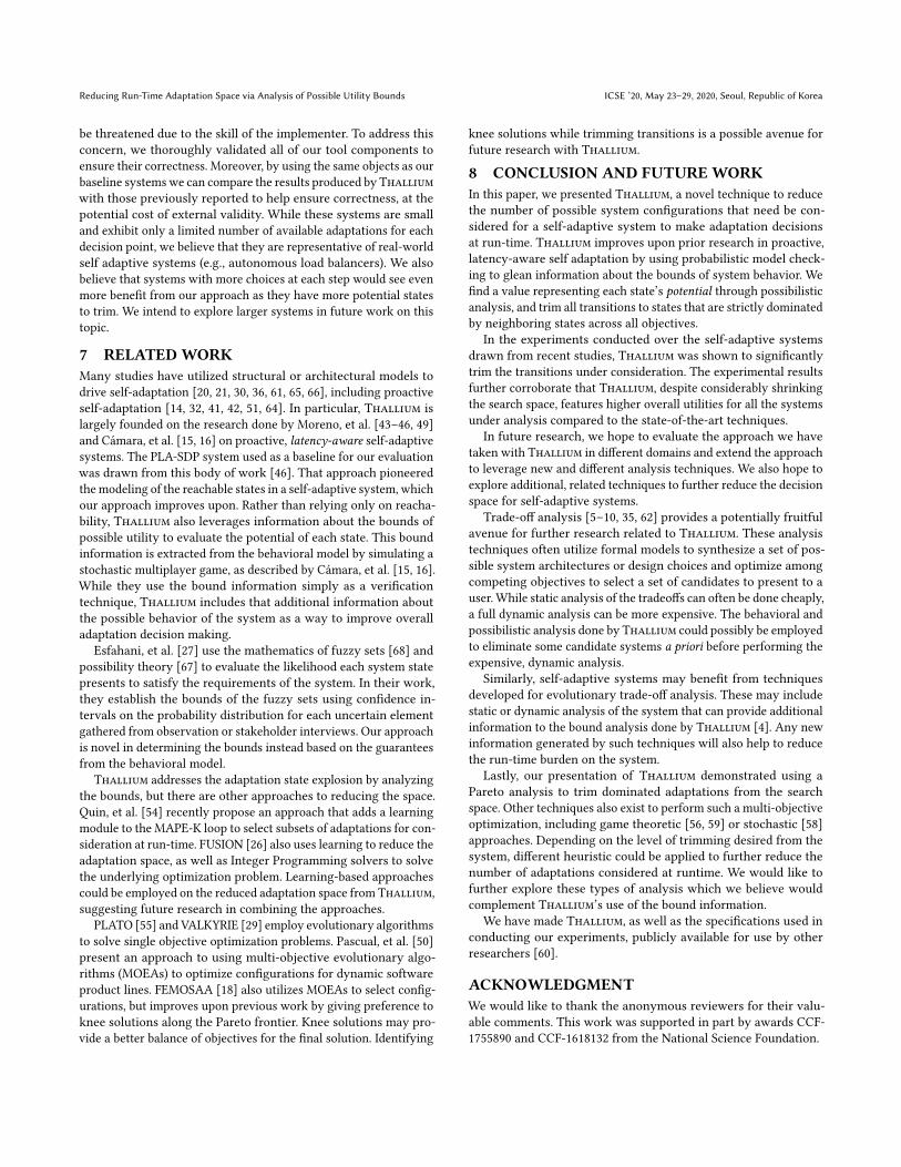
Figure 13: Comparing Thallium and the state-of-the-art

PLA-SDP technique for the SWIM self-adaptive system [48].

Thallium (a) reduces the number of adaptations considered

by 51.9%, and (b) achieves higher cumulative utility.

For the SWIM exemplar, PLA-SDP generated a total of 340 possi-ble system configurations, connected by 1,172 admissible adapta-tions. The model provided to the Utility Bounds Analysis componentwas drawn from a real-world trace of TCP activity published byClarkNet [3] which fluctuated between 0 and 130 requests per pe-riod. Thallium trimmed between 640 and 756 adaptations fromconsideration, reducing the adaptation space by between 54.6% and64.5% (as shown in Figure 12). Averaged across all weight settings,Thallium reduced the number of adaptations for SWIM by 63.2%.For DART, PLA-SDP devised 80 system configuration states with112 admissible adaptations; Thallium reduced that number by anaverage of 21.9%, trimming between 16 and 28 adaptations.

Overall, the differing weights in all cases produced only a smallvariation in the number of adaptations trimmed from the baselineMDP, consistently hewing close to the mean. For SWIM, the relativestandard error in the percentage of adaptations trimmed across all16 weightings was only 1%; for DART, it was 4%. For each weighting

evaluated, Thallium consistently trimmed adaptations when com-

pared to PLA-SDP, and all of the tests across all the subject systems

resulted in a reduction of the adaptation space.

4.4 Experiment 2: SWIM Simulation

Our second experiment evaluated Thallium’s impact at run-timethrough the use of the SWIM network simulator. The experimentmeasures two values: (1) the number of adaptations evaluated as

part of each adaptation decision and (2) the overall cumulativeutility reported by the simulator. The results for both measurementsare summarized in Figure 13.

For the first number of adaptations evaluated, we found large dif-ferences in the number of run -time comparisons performed usingeach approach during adaptation decisions. Figure 13(a) shows thenumber of joint system/environment states to which adaptationwas evaluated. The adaptation manager based on PLA-SDP aver-aged 99,989 comparisons per adaptation decision. This number ismuch higher than the 1,172 adaptations present in the system MDPgenerated by PLA-SDP, as the look-ahead done by the proactivemanager and the uncertainty in intertwined environmental statesballoons that number in order to fully evaluate each possible adap-tation at run-time. Thallium cuts that number in half, to 48,108run-time comparisons (a reduction of 51.9%) for each adaptationdecision.

Figure 13(b) summarizes the overall system utility determinedby the SWIM simulator for PLA-SDP and Thallium. PLA-SDPgenerated a cumulative utility value of 4,067 over the course ofthe trace, while Thallium achieved a higher cumulative utilitytotal, with a final tally of 4,692. The difference in the observedcumulative utility between PLA-SDP and Thallium becomes moreand more pronounced as the execution time increases. AlongsidePLA-SDP and Thallium, we also assessed a third, purely reactiveadaptationmechanism [43] that responded to the observed responsetime (not shown). The reactive manager frequently violated the 750millisecond response time threshold imposed by the simulator’sutility function, resulting in a negative cumulative utility due to theaccrued penalties.

4.5 Experiment 3: DART Simulation

Our third experiment evaluated Thallium’s impact at run-timethrough the use of the DARTSim simulator [47] of the DART system.The simulator plotted the course of a drone team over a randomly-generated, 40-step course containing four targets and six threats,allowing the drones to adopt two formations and one of five alti-tudes.

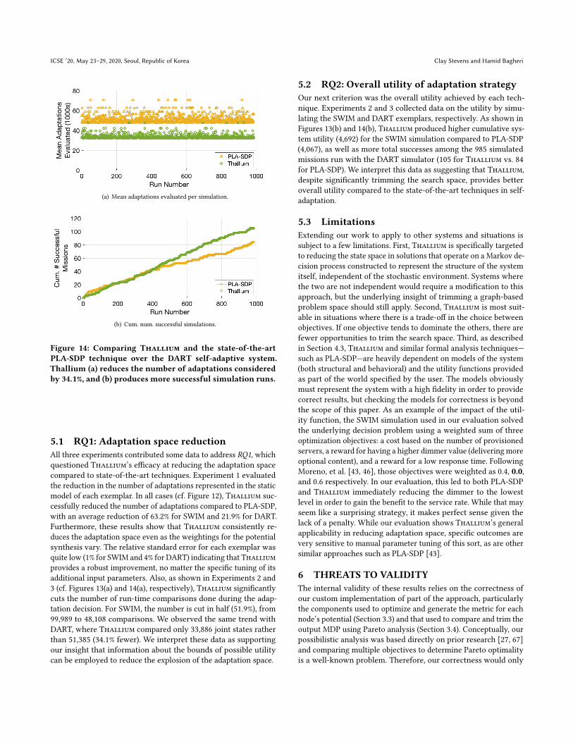
Figure 14 depicts the results of experiments conducted over 985such courses. According to the experimental results, a remarkablereduction in the number of adaptations evaluated at run-time isobserved when using Thallium. DART with PLA-SDP performed51,385 comparisons per evaluation (on average) across the 39,400simulated evaluation periods, whereas Thallium compared anaverage of only 33,886 joint states (34.1% fewer).

For overall utility, DART determines whether or not each mis-sion was an overall success, i.e., the team was not destroyed and itdetected at least half of the targets. Figure 14(b) summarizes the suc-cessful missions by both PLA-SDP and Thallium. The success rateachieved by Thallium is noticeably higher than that of PLA-SDP.Specifically, out of the 985 runs, PLA-SDP resulted in 84 successfulmissions total, whereas Thallium was successful in 105.

5 DISCUSSION

This section details our interpretation of the results obtained withrespect to each research question and presents some limitations.

ICSE ’20, May 23–29, 2020, Seoul, Republic of Korea Clay Stevens and Hamid Bagheri

(a) Mean adaptations evaluated per simulation.

(b) Cum. num. successful simulations.

Figure 14: Comparing Thallium and the state-of-the-art

PLA-SDP technique over the DART self-adaptive system.

Thallium (a) reduces the number of adaptations considered

by 34.1%, and (b) produces more successful simulation runs.

5.1 RQ1: Adaptation space reduction

All three experiments contributed some data to address RQ1, whichquestioned Thallium’s efficacy at reducing the adaptation spacecompared to state-of-the-art techniques. Experiment 1 evaluatedthe reduction in the number of adaptations represented in the staticmodel of each exemplar. In all cases (cf. Figure 12), Thallium suc-cessfully reduced the number of adaptations compared to PLA-SDP,with an average reduction of 63.2% for SWIM and 21.9% for DART.Furthermore, these results show that Thallium consistently re-duces the adaptation space even as the weightings for the potentialsynthesis vary. The relative standard error for each exemplar wasquite low (1% for SWIM and 4% for DART) indicating that Thalliumprovides a robust improvement, no matter the specific tuning of itsadditional input parameters. Also, as shown in Experiments 2 and3 (cf. Figures 13(a) and 14(a), respectively), Thallium significantlycuts the number of run-time comparisons done during the adap-tation decision. For SWIM, the number is cut in half (51.9%), from99,989 to 48,108 comparisons. We observed the same trend withDART, where Thallium compared only 33,886 joint states ratherthan 51,385 (34.1% fewer). We interpret these data as supportingour insight that information about the bounds of possible utilitycan be employed to reduce the explosion of the adaptation space.

5.2 RQ2: Overall utility of adaptation strategy

Our next criterion was the overall utility achieved by each tech-nique. Experiments 2 and 3 collected data on the utility by simu-lating the SWIM and DART exemplars, respectively. As shown inFigures 13(b) and 14(b), Thallium produced higher cumulative sys-tem utility (4,692) for the SWIM simulation compared to PLA-SDP(4,067), as well as more total successes among the 985 simulatedmissions run with the DART simulator (105 for Thallium vs. 84for PLA-SDP). We interpret this data as suggesting that Thallium,despite significantly trimming the search space, provides betteroverall utility compared to the state-of-the-art techniques in self-adaptation.

5.3 Limitations

Extending our work to apply to other systems and situations issubject to a few limitations. First, Thallium is specifically targetedto reducing the state space in solutions that operate on a Markov de-cision process constructed to represent the structure of the systemitself, independent of the stochastic environment. Systems wherethe two are not independent would require a modification to thisapproach, but the underlying insight of trimming a graph-basedproblem space should still apply. Second, Thallium is most suit-able in situations where there is a trade-off in the choice betweenobjectives. If one objective tends to dominate the others, there arefewer opportunities to trim the search space. Third, as describedin Section 4.3, Thallium and similar formal analysis techniques—such as PLA-SDP—are heavily dependent on models of the system(both structural and behavioral) and the utility functions providedas part of the world specified by the user. The models obviouslymust represent the system with a high fidelity in order to providecorrect results, but checking the models for correctness is beyondthe scope of this paper. As an example of the impact of the util-ity function, the SWIM simulation used in our evaluation solvedthe underlying decision problem using a weighted sum of threeoptimization objectives: a cost based on the number of provisionedservers, a reward for having a higher dimmer value (deliveringmoreoptional content), and a reward for a low response time. FollowingMoreno, et al. [43, 46], those objectives were weighted as 0.4, 0.0,and 0.6 respectively. In our evaluation, this led to both PLA-SDPand Thallium immediately reducing the dimmer to the lowestlevel in order to gain the benefit to the service rate. While that mayseem like a surprising strategy, it makes perfect sense given thelack of a penalty. While our evaluation shows Thallium’s generalapplicability in reducing adaptation space, specific outcomes arevery sensitive to manual parameter tuning of this sort, as are othersimilar approaches such as PLA-SDP [43].

6 THREATS TO VALIDITY

The internal validity of these results relies on the correctness ofour custom implementation of part of the approach, particularlythe components used to optimize and generate the metric for eachnode’s potential (Section 3.3) and that used to compare and trim theoutput MDP using Pareto analysis (Section 3.4). Conceptually, ourpossibilistic analysis was based directly on prior research [27, 67]and comparing multiple objectives to determine Pareto optimalityis a well-known problem. Therefore, our correctness would only

Reducing Run-Time Adaptation Space via Analysis of Possible Utility Bounds ICSE ’20, May 23–29, 2020, Seoul, Republic of Korea

be threatened due to the skill of the implementer. To address thisconcern, we thoroughly validated all of our tool components toensure their correctness. Moreover, by using the same objects as ourbaseline systemswe can compare the results produced by Thalliumwith those previously reported to help ensure correctness, at thepotential cost of external validity. While these systems are smalland exhibit only a limited number of available adaptations for eachdecision point, we believe that they are representative of real-worldself adaptive systems (e.g., autonomous load balancers). We alsobelieve that systems with more choices at each step would see evenmore benefit from our approach as they have more potential statesto trim. We intend to explore larger systems in future work on thistopic.

7 RELATEDWORK

Many studies have utilized structural or architectural models todrive self-adaptation [20, 21, 30, 36, 61, 65, 66], including proactiveself-adaptation [14, 32, 41, 42, 51, 64]. In particular, Thallium islargely founded on the research done by Moreno, et al. [43–46, 49]and Cámara, et al. [15, 16] on proactive, latency-aware self-adaptivesystems. The PLA-SDP system used as a baseline for our evaluationwas drawn from this body of work [46]. That approach pioneeredthemodeling of the reachable states in a self-adaptive system, whichour approach improves upon. Rather than relying only on reacha-bility, Thallium also leverages information about the bounds ofpossible utility to evaluate the potential of each state. This boundinformation is extracted from the behavioral model by simulating astochastic multiplayer game, as described by Cámara, et al. [15, 16].While they use the bound information simply as a verificationtechnique, Thallium includes that additional information aboutthe possible behavior of the system as a way to improve overalladaptation decision making.

Esfahani, et al. [27] use the mathematics of fuzzy sets [68] andpossibility theory [67] to evaluate the likelihood each system statepresents to satisfy the requirements of the system. In their work,they establish the bounds of the fuzzy sets using confidence in-tervals on the probability distribution for each uncertain elementgathered from observation or stakeholder interviews. Our approachis novel in determining the bounds instead based on the guaranteesfrom the behavioral model.

Thallium addresses the adaptation state explosion by analyzingthe bounds, but there are other approaches to reducing the space.Quin, et al. [54] recently propose an approach that adds a learningmodule to the MAPE-K loop to select subsets of adaptations for con-sideration at run-time. FUSION [26] also uses learning to reduce theadaptation space, as well as Integer Programming solvers to solvethe underlying optimization problem. Learning-based approachescould be employed on the reduced adaptation space from Thallium,suggesting future research in combining the approaches.

PLATO [55] and VALKYRIE [29] employ evolutionary algorithmsto solve single objective optimization problems. Pascual, et al. [50]present an approach to using multi-objective evolutionary algo-rithms (MOEAs) to optimize configurations for dynamic softwareproduct lines. FEMOSAA [18] also utilizes MOEAs to select config-urations, but improves upon previous work by giving preference toknee solutions along the Pareto frontier. Knee solutions may pro-vide a better balance of objectives for the final solution. Identifying

knee solutions while trimming transitions is a possible avenue forfuture research with Thallium.

8 CONCLUSION AND FUTUREWORK

In this paper, we presented Thallium, a novel technique to reducethe number of possible system configurations that need be con-sidered for a self-adaptive system to make adaptation decisionsat run-time. Thallium improves upon prior research in proactive,latency-aware self adaptation by using probabilistic model check-ing to glean information about the bounds of system behavior. Wefind a value representing each state’s potential through possibilisticanalysis, and trim all transitions to states that are strictly dominatedby neighboring states across all objectives.

In the experiments conducted over the self-adaptive systemsdrawn from recent studies, Thallium was shown to significantlytrim the transitions under consideration. The experimental resultsfurther corroborate that Thallium, despite considerably shrinkingthe search space, features higher overall utilities for all the systemsunder analysis compared to the state-of-the-art techniques.

In future research, we hope to evaluate the approach we havetaken with Thallium in different domains and extend the approachto leverage new and different analysis techniques. We also hope toexplore additional, related techniques to further reduce the decisionspace for self-adaptive systems.

Trade-off analysis [5–10, 35, 62] provides a potentially fruitfulavenue for further research related to Thallium. These analysistechniques often utilize formal models to synthesize a set of pos-sible system architectures or design choices and optimize amongcompeting objectives to select a set of candidates to present to auser. While static analysis of the tradeoffs can often be done cheaply,a full dynamic analysis can be more expensive. The behavioral andpossibilistic analysis done by Thallium could possibly be employedto eliminate some candidate systems a priori before performing theexpensive, dynamic analysis.

Similarly, self-adaptive systems may benefit from techniquesdeveloped for evolutionary trade-off analysis. These may includestatic or dynamic analysis of the system that can provide additionalinformation to the bound analysis done by Thallium [4]. Any newinformation generated by such techniques will also help to reducethe run-time burden on the system.

Lastly, our presentation of Thallium demonstrated using aPareto analysis to trim dominated adaptations from the searchspace. Other techniques also exist to perform such a multi-objectiveoptimization, including game theoretic [56, 59] or stochastic [58]approaches. Depending on the level of trimming desired from thesystem, different heuristic could be applied to further reduce thenumber of adaptations considered at runtime. We would like tofurther explore these types of analysis which we believe wouldcomplement Thallium’s use of the bound information.

We have made Thallium, as well as the specifications used inconducting our experiments, publicly available for use by otherresearchers [60].

ACKNOWLEDGMENT

We would like to thank the anonymous reviewers for their valu-able comments. This work was supported in part by awards CCF-1755890 and CCF-1618132 from the National Science Foundation.

ICSE ’20, May 23–29, 2020, Seoul, Republic of Korea Clay Stevens and Hamid Bagheri

REFERENCES

[1] Jonathan Aldrich, David Garlan, Christian Kästner, Claire Le Goues, AnahitaMohseni-Kabir, Ivan Ruchkin, Selva Samuel, Bradley R. Schmerl, Christo-pher Steven Timperley, Manuela Veloso, Ian Voysey, Joydeep Biswas, ArjunGuha, Jarrett Holtz, Javier Cámara, and Pooyan Jamshidi. 2019. Model-BasedAdaptation for Robotics Software. IEEE Software 36, 2 (2019), 83–90. https://doi.org/10.1109/MS.2018.2885058

[2] Rajeev Alur, Thomas A. Henzinger, and Orna Kupferman. 2002. Alternating-timetemporal logic. J. ACM 49, 5 (2002), 672–713. https://doi.org/10.1145/585265.585270

[3] Martin Arlitt and Carey Williamson. 2004. Clark-Net HTTP. (2004). http://ita.ee.lbl.gov/html/contrib/ClarkNet-HTTP.html

[4] Hamid Bagheri and SamMalek. 2016. Titanium: efficient analysis of evolving alloyspecifications. In Proceedings of the 24th ACM SIGSOFT International Symposium

on Foundations of Software Engineering, FSE 2016, Seattle, WA, USA, November

13-18, 2016, Thomas Zimmermann, Jane Cleland-Huang, and Zhendong Su (Eds.).ACM, 27–38. https://doi.org/10.1145/2950290.2950337

[5] Hamid Bagheri, Yuanyuan Song, and Kevin J. Sullivan. 2010. Architectural styleas an independent variable. In ASE 2010, 25th IEEE/ACM International Conference

on Automated Software Engineering, Antwerp, Belgium, September 20-24, 2010,Charles Pecheur, Jamie Andrews, and Elisabetta Di Nitto (Eds.). ACM, 159–162.https://doi.org/10.1145/1858996.1859026

[6] Hamid Bagheri and Kevin J. Sullivan. 2010. Monarch: Model-Based Developmentof Software Architectures. In Model Driven Engineering Languages and Systems

- 13th International Conference, MODELS 2010, Oslo, Norway, October 3-8, 2010,

Proceedings, Part II (Lecture Notes in Computer Science), Dorina C. Petriu, NicolasRouquette, and Øystein Haugen (Eds.), Vol. 6395. Springer, 376–390. https://doi.org/10.1007/978-3-642-16129-2_27

[7] Hamid Bagheri and Kevin J. Sullivan. 2016. Model-driven synthesis of formallyprecise, stylized software architectures. Formal Asp. Comput. 28, 3 (2016), 441–467.https://doi.org/10.1007/s00165-016-0360-8

[8] Hamid Bagheri, Kevin J. Sullivan, and Sang H. Son. 2012. Spacemaker: PracticalFormal Synthesis of Tradeoff Spaces for Object-Relational Mapping. In Proceed-

ings of the 24th International Conference on Software Engineering & Knowledge

Engineering (SEKE’2012), Hotel Sofitel, Redwood City, San Francisco Bay, USA July

1-3, 2012. Knowledge Systems Institute Graduate School, 688–693.[9] Hamid Bagheri, Chong Tang, and Kevin J. Sullivan. 2014. TradeMaker: automated

dynamic analysis of synthesized tradespaces. In 36th International Conference

on Software Engineering, ICSE ’14, Hyderabad, India - May 31 - June 07, 2014,Pankaj Jalote, Lionel C. Briand, and André van der Hoek (Eds.). ACM, 106–116.https://doi.org/10.1145/2568225.2568291

[10] Hamid Bagheri, Chong Tang, and Kevin J. Sullivan. 2017. Automated Synthesisand Dynamic Analysis of Tradeoff Spaces for Object-Relational Mapping. IEEETrans. Software Eng. 43, 2 (2017), 145–163. https://doi.org/10.1109/TSE.2016.2587646

[11] Richard Bellman. 2010. Dynamic Programming. Princeton University Press,Princeton, NJ, USA.

[12] Craig Boutilier, Ronen I. Brafman, and Christopher Geib. 1998. Structured Reach-ability Analysis for Markov Decision Processes. In Proceedings of the Fourteenth

Conference on Uncertainty in Artificial Intelligence (UAI’98). Morgan KaufmannPublishers Inc., San Francisco, CA, USA, 24–32. http://dl.acm.org/citation.cfm?id=2074094.2074098

[13] Radu Calinescu, Simos Gerasimou, and Alec Banks. 2015. Self-adaptive Softwarewith Decentralised Control Loops. In Fundamental Approaches to Software Engi-

neering - 18th International Conference, FASE 2015, Held as Part of the European

Joint Conferences on Theory and Practice of Software, ETAPS 2015, London, UK, April

11-18, 2015. Proceedings (Lecture Notes in Computer Science), Alexander Egyedand Ina Schaefer (Eds.), Vol. 9033. Springer, 235–251. https://doi.org/10.1007/978-3-662-46675-9_16

[14] Radu Calinescu, Lars Grunske, Marta Z. Kwiatkowska, Raffaela Mirandola, andGiordano Tamburrelli. 2011. Dynamic QoS Management and Optimization inService-Based Systems. IEEE Trans. Software Eng. 37, 3 (2011), 387–409. https://doi.org/10.1109/TSE.2010.92

[15] Javier Cámara, Gabriel A. Moreno, and David Garlan. 2014. Stochastic GameAnalysis and Latency Awareness for Proactive Self-adaptation. In Proceedings

of the 9th International Symposium on Software Engineering for Adaptive and

Self-Managing Systems (SEAMS 2014). ACM, New York, NY, USA, 155–164. https://doi.org/10.1145/2593929.2593933

[16] Javier Cámara, Gabriel A. Moreno, David Garlan, and Bradley Schmerl. 2016.Analyzing Latency-Aware Self-Adaptation Using Stochastic and Simulations.ACM Trans. Auton. Adapt. Syst. 10, 4, Article 23 (Jan. 2016), 28 pages. https://doi.org/10.1145/2774222

[17] T. Chen, V. Forejt, M. Kwiatkowska, D. Parker, and A. Simaitis. 2013. AutomaticVerification of Competitive Stochastic Systems. Formal Methods in System Design

43, 1 (2013), 61–92.[18] Tao Chen, Ke Li, Rami Bahsoon, and Xin Yao. 2018. FEMOSAA: Feature-Guided

and Knee-Driven Multi-Objective Optimization for Self-Adaptive Software. ACM

Trans. Softw. Eng. Methodol. 27, 2, Article 5 (June 2018), 50 pages. https://doi.org/10.1145/3204459

[19] Betty H. C. Cheng, Rogério de Lemos, Holger Giese, Paola Inverardi, and JeffMagee (Eds.). 2009. Software Engineering for Self-Adaptive Systems: A Research

Roadmap. Springer Berlin Heidelberg, Berlin, Heidelberg, 1–26. https://doi.org/10.1007/978-3-642-02161-9_1

[20] Shang-Wen Cheng and David Garlan. 2012. Stitch: A language for architecture-based self-adaptation. Journal of Systems and Software 85, 12 (2012), 2860–2875.https://doi.org/10.1016/j.jss.2012.02.060

[21] Shang-Wen Cheng, Vahe Poladian, David Garlan, and Bradley R. Schmerl. 2009.Improving Architecture-Based Self-Adaptation through Resource Prediction. InSoftware Engineering for Self-Adaptive Systems [outcome of a Dagstuhl Seminar].71–88. https://doi.org/10.1007/978-3-642-02161-9_4

[22] Philipp Chrszon, Clemens Dubslaff, Sascha Klüppelholz, and Christel Baier. 2018.ProFeat: feature-oriented engineering for family-based probabilistic model check-ing. Formal Asp. Comput. 30, 1 (2018), 45–75. https://doi.org/10.1007/s00165-017-0432-4

[23] Zack Coker, David Garlan, and Claire Le Goues. 2015. SASS: Self-AdaptationUsing Stochastic Search. In 10th IEEE/ACM International Symposium on Software

Engineering for Adaptive and Self-Managing Systems, SEAMS 2015, Florence, Italy,

May 18-19, 2015, Paola Inverardi and Bradley R. Schmerl (Eds.). IEEE ComputerSociety, 168–174. https://doi.org/10.1109/SEAMS.2015.16

[24] Rogério de Lemos, Holger Giese, Hausi A. Müller, and Mary Shaw (Eds.). 2013.Software Engineering for Self-Adaptive Systems: A Second Research Roadmap.Springer Berlin Heidelberg, Berlin, Heidelberg, 1–32. https://doi.org/10.1007/978-3-642-35813-5_1

[25] Ahmed M. Elkhodary, Naeem Esfahani, and Sam Malek. 2010. FUSION: a frame-work for engineering self-tuning self-adaptive software systems. In Proceedings ofthe 18th ACM SIGSOFT International Symposium on Foundations of Software Engi-

neering, 2010, Santa Fe, NM, USA, November 7-11, 2010, Gruia-Catalin Roman andAndré van der Hoek (Eds.). ACM, 7–16. https://doi.org/10.1145/1882291.1882296

[26] N. Esfahani, A. Elkhodary, and S. Malek. 2013. A Learning-Based Framework forEngineering Feature-Oriented Self-Adaptive Software Systems. IEEE Transactionson Software Engineering 39, 11 (Nov 2013), 1467–1493. https://doi.org/10.1109/TSE.2013.37

[27] Naeem Esfahani, Ehsan Kouroshfar, and SamMalek. 2011. Taming Uncertainty inSelf-adaptive Software. In Proceedings of the 19th ACM SIGSOFT Symposium and

the 13th European Conference on Foundations of Software Engineering (ESEC/FSE

’11). ACM, New York, NY, USA, 234–244. https://doi.org/10.1145/2025113.2025147[28] V. Forejt, M. Kwiatkowska, G. Norman, and D. Parker. 2011. Automated Ver-

ification Techniques for Probabilistic Systems. In Formal Methods for Eternal

Networked Software Systems (SFM’11) (LNCS), M. Bernardo and V. Issarny (Eds.),Vol. 6659. Springer, 53–113.

[29] ErikM. Fredericks. 2016. Automatically Hardening a Self-adaptive SystemAgainstUncertainty. In Proceedings of the 11th International Symposium on Software

Engineering for Adaptive and Self-Managing Systems (SEAMS ’16). ACM, NewYork, NY, USA, 16–27. https://doi.org/10.1145/2897053.2897059

[30] David Garlan, Shang-Wen Cheng, An-Cheng Huang, Bradley Schmerl, and PeterSteenkiste. 2004. Rainbow: Architecture-Based Self-Adaptation with ReusableInfrastructure. Computer 37, 10 (Oct. 2004), 46–54. https://doi.org/10.1109/MC.2004.175

[31] Robert Givan, Thomas Dean, and Matthew Greig. 2003. Equivalence Notions andModel Minimization in Markov Decision Processes. Artif. Intell. 147, 1-2 (July2003), 163–223. https://doi.org/10.1016/S0004-3702(02)00376-4

[32] Julia Hielscher, Raman Kazhamiakin, Andreas Metzger, and Marco Pistore. 2008.A Framework for Proactive Self-adaptation of Service-Based Applications Basedon Online Testing. In Towards a Service-Based Internet, First European Conference,

ServiceWave 2008, Madrid, Spain, December 10-13, 2008. Proceedings. 122–133.https://doi.org/10.1007/978-3-540-89897-9_11

[33] Scott A. Hissam, Sagar Chaki, and Gabriel A. Moreno. 2015. High Assurancefor Distributed Cyber Physical Systems. In Proceedings of the 2015 European

Conference on Software Architecture Workshops (ECSAW ’15). ACM, New York,NY, USA, Article 6, 4 pages. https://doi.org/10.1145/2797433.2797439

[34] Daniel Jackson. 2002. Alloy: A Lightweight Object Modelling Notation. ACMTrans. Softw. Eng. Methodol. 11, 2 (April 2002), 256–290. https://doi.org/10.1145/505145.505149

[35] Jung Soo Kim and David Garlan. 2010. Analyzing architectural styles. Journal ofSystems and Software 83, 7 (2010), 1216–1235. https://doi.org/10.1016/j.jss.2010.01.049

[36] Christian Krupitzer, Felix Maximilian Roth, Sebastian VanSyckel, Gregor Schiele,and Christian Becker. 2015. A Survey on Engineering Approaches for Self-adaptive Systems. Pervasive Mob. Comput. 17, PB (Feb. 2015), 184–206. https://doi.org/10.1016/j.pmcj.2014.09.009

[37] M. Kwiatkowska, G. Norman, and D. Parker. 2011. PRISM 4.0: Verification ofProbabilistic Real-time Systems. In Proc. 23rd International Conference on Com-

puter Aided Verification (CAV’11) (LNCS), G. Gopalakrishnan and S. Qadeer (Eds.),Vol. 6806. Springer, 585–591.

Reducing Run-Time Adaptation Space via Analysis of Possible Utility Bounds ICSE ’20, May 23–29, 2020, Seoul, Republic of Korea

[38] Young-Jou Lai and Ching-Lai Hwang. 1992. ANewApproach to Some PossibilisticLinear Programming Problems. Fuzzy Sets Syst. 49, 2 (July 1992), 121–133. https://doi.org/10.1016/0165-0114(92)90318-X

[39] Marin Litoiu, Siobhán Clarke, and Kenji Tei (Eds.). 2019. Proceedings of the

14th International Symposium on Software Engineering for Adaptive and Self-

Managing Systems, SEAMS@ICSE 2019, Montreal, QC, Canada, May 25-31, 2019.ACM. https://dl.acm.org/citation.cfm?id=3341527

[40] Ming Mao and Marty Humphrey. 2012. A Performance Study on the VM StartupTime in the Cloud. In Proceedings of the 2012 IEEE Fifth International Conference

on Cloud Computing (CLOUD ’12). IEEE Computer Society, Washington, DC, USA,423–430. https://doi.org/10.1109/CLOUD.2012.103

[41] Andreas Metzger and Philipp Bohn. 2017. Risk-Based Proactive Process Adapta-tion. In Service-Oriented Computing - 15th International Conference, ICSOC 2017,

Malaga, Spain, November 13-16, 2017, Proceedings. 351–366. https://doi.org/10.1007/978-3-319-69035-3_25

[42] Andreas Metzger, Osama Sammodi, and Klaus Pohl. 2013. Accurate ProactiveAdaptation of Service-Oriented Systems. In Assurances for Self-Adaptive Systems

- Principles, Models, and Techniques. 240–265. https://doi.org/10.1007/978-3-642-36249-1_9

[43] Gabriel A. Moreno. 2017. Adaptation Timing in Self-Adaptive Systems. Ph.D.Dissertation. School of Comp. Sci., Carnegie Mellon Univ., Pittsburgh, PA.

[44] Gabriel A. Moreno, Javier Cámara, David Garlan, and Bradley Schmerl. 2015.Proactive Self-adaptation Under Uncertainty: A Probabilistic Model CheckingApproach. In Proceedings of the 2015 10th Joint Meeting on Foundations of Software

Engineering (ESEC/FSE 2015). ACM, New York, NY, USA, 1–12. https://doi.org/10.1145/2786805.2786853

[45] Gabriel A. Moreno, Javier Cámara, David Garlan, and Bradley Schmerl. 2016.Efficient Decision-Making under Uncertainty for Proactive Self-Adaptation. In2016 IEEE International Conference on Autonomic Computing (ICAC). 147–156.https://doi.org/10.1109/ICAC.2016.59

[46] Gabriel A. Moreno, Javier Cámara, David Garlan, and Bradley Schmerl. 2018. Flex-ible and Efficient Decision-Making for Proactive Latency-Aware Self-Adaptation.ACM Trans. Auton. Adapt. Syst. 13, 1, Article 3 (April 2018), 36 pages. https://doi.org/10.1145/3149180

[47] Gabriel A. Moreno, Cody Kinneer, Ashutosh Pandey, and David Garlan. 2019.DARTSim: an exemplar for evaluation and comparison of self-adaptation ap-proaches for smart cyber-physical systems, See [39], 181–187. https://dl.acm.org/citation.cfm?id=3341554

[48] Gabriel A. Moreno, Bradley Schmerl, and David Garlan. 2018. SWIM: An Ex-emplar for Evaluation and Comparison of Self-adaptation Approaches for WebApplications. In Proceedings of the 13th International Conference on Software Engi-

neering for Adaptive and Self-Managing Systems (SEAMS ’18). ACM, New York,NY, USA, 137–143. https://doi.org/10.1145/3194133.3194163

[49] Gabriel A. Moreno, Ofer Strichman, Sagar Chaki, and Radislav Vaisman. 2017.Decision-making with Cross-entropy for Self-adaptation. In Proceedings of the

12th International Symposium on Software Engineering for Adaptive and Self-

Managing Systems (SEAMS ’17). IEEE Press, Piscataway, NJ, USA, 90–101. https://doi.org/10.1109/SEAMS.2017.7

[50] Gustavo G. Pascual, Roberto E. Lopez-Herrejon, Mónica Pinto, Lidia Fuentes, andAlexander Egyed. 2015. Applying Multiobjective Evolutionary Algorithms toDynamic Software Product Lines for Reconfiguring Mobile Applications. J. Syst.Softw. 103, C (May 2015), 392–411. https://doi.org/10.1016/j.jss.2014.12.041

[51] V. Poladian, D. Garlan, M. Shaw, M. Satyanarayanan, B. Schmerl, and J. Sousa.2007. Leveraging Resource Prediction for Anticipatory Dynamic Configuration.In First International Conference on Self-Adaptive and Self-Organizing Systems

(SASO 2007). 214–223. https://doi.org/10.1109/SASO.2007.35[52] prism doc 2019. PRISM Documentation. https://www.prismmodelchecker.org/

doc/. (2019).[53] Martin L. Puterman. 1994. Markov Decision Processes: Discrete Stochastic Dynamic

Programming (1st ed.). John Wiley & Sons, Inc., New York, NY, USA.[54] Federico Quin, Danny Weyns, Thomas Bamelis, Sarpreet Singh Buttar, and Sam

Michiels. 2019. Efficient analysis of large adaptation spaces in self-adaptivesystems using machine learning, See [39], 1–12. https://dl.acm.org/citation.cfm?id=3341529

[55] Andres J. Ramirez, David B. Knoester, Betty H. C. Cheng, and Philip K. McKinley.2011. Plato: a genetic algorithm approach to run-time reconfiguration inÂăau-tonomic computing systems. Cluster Computing 14, 3 (01 Sep 2011), 229–244.https://doi.org/10.1007/s10586-010-0122-y

[56] Rui Meng, Ye Ye, and Neng-gang Xie. 2010. Multi-objective optimization designmethods based on game theory. In 2010 8th World Congress on Intelligent Control

and Automation. 2220–2227. https://doi.org/10.1109/WCICA.2010.5554307[57] Mazeiar Salehie and Ladan Tahvildari. 2009. Self-adaptive Software: Landscape

and Research Challenges. ACM Trans. Auton. Adapt. Syst. 4, 2, Article 14 (May2009), 42 pages. https://doi.org/10.1145/1516533.1516538

[58] S. B. Selcuklu, D. W. Coit, F. Felder, M. Rodgers, and N. Wattanapongsakorn. 2013.A new methodology for solving multi-objective stochastic optimization problemswith independent objective functions. In 2013 IEEE International Conference on

Industrial Engineering and Engineering Management. 101–105. https://doi.org/10.1109/IEEM.2013.6962383

[59] Kwee-Bo Sim, Ji-Yoon Kim, and Dong-Wook Lee. 2004. Game Theory BasedCo-evolutionary Algorithm (GCEA) for Solving Multiobjective OptimizationProblems. IEICE Transactions 87-D, 10 (2004), 2419–2425. http://search.ieice.org/bin/summary.php?id=e87-d_10_2419

[60] Clay Stevens and Hamid Bagheri. 2019. Thallium Website. https://sites.google.com/view/thallium/. (2019).

[61] Jacob Swanson, Myra B. Cohen, Matthew B. Dwyer, Brady J. Garvin, and JustinFirestone. 2014. Beyond the Rainbow: Self-adaptive Failure Avoidance in Config-urable Systems. In Proceedings of the 22Nd ACM SIGSOFT International Symposium

on Foundations of Software Engineering (FSE 2014). ACM, New York, NY, USA,377–388. https://doi.org/10.1145/2635868.2635915

[62] Chong Tang, Hamid Bagheri, Sarun Paisarnsrisomsuk, and Kevin J. Sullivan. 2017.Towards designing effective data persistence through tradeoff space analysis. InProceedings of the 39th International Conference on Software Engineering, ICSE

2017, Buenos Aires, Argentina, May 20-28, 2017 - Companion Volume, SebastiánUchitel, Alessandro Orso, and Martin P. Robillard (Eds.). IEEE Computer Society,353–355. https://doi.org/10.1109/ICSE-C.2017.106

[63] András Varga and Rudolf Hornig. 2008. AnOverview of the OMNeT++ SimulationEnvironment. In Proceedings of the 1st International Conference on Simulation

Tools and Techniques for Communications, Networks and Systems & Workshops

(Simutools ’08). ICST (Institute for Computer Sciences, Social-Informatics andTelecommunications Engineering), ICST, Brussels, Belgium, Belgium, Article 60,10 pages. http://dl.acm.org/citation.cfm?id=1416222.1416290

[64] ChenWang and Jean-Louis Pazat. 2012. A Two-Phase Online PredictionApproachfor Accurate and Timely Adaptation Decision. In 2012 IEEE Ninth International

Conference on Services Computing, Honolulu, HI, USA, June 24-29, 2012. 218–225.https://doi.org/10.1109/SCC.2012.26

[65] DannyWeyns. 2018. Engineering Self-Adaptive Software Systems - An OrganizedTour. In 2018 IEEE 3rd International Workshops on Foundations and Applications of

Self* Systems (FAS*W), Trento, Italy, September 3-7, 2018. 1–2. https://doi.org/10.1109/FAS-W.2018.00012

[66] Danny Weyns, Sam Malek, Rogério de Lemos, and Jesper Andersson (Eds.).2010. Self-Organizing Architectures, First International Workshop, SOAR 2009,

Cambridge, UK, September 14, 2009, Revised Selected and Invited Papers. LectureNotes in Computer Science, Vol. 6090. Springer. https://doi.org/10.1007/978-3-642-14412-7

[67] L. A. Zadeh. 1999. Fuzzy Sets As a Basis for a Theory of Possibility. Fuzzy Sets

Syst. 100 (April 1999), 9–34. http://dl.acm.org/citation.cfm?id=310817.310820[68] H.-J. Zimmermann. 1996. Fuzzy Set Theory&Mdash;and Its Applications (3rd Ed.).

Kluwer Academic Publishers, Norwell, MA, USA.