reducing noc energy consumption through compiler-directed channel voltage scaling guangyu chen,...

Reducing NoC Energy Consumption Through Compiler-Directed Channel Voltage Scaling

Guangyu Chen, Feihui Li, Mahmut Kandemir, Mary Jane Irwin

Microsystems Design Lab, Department of CSE

The Pennsylvania State University

[email protected]

PLDI’06 2

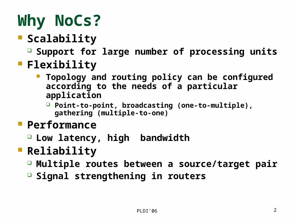
Why NoCs? Scalability

Support for large number of processing units Flexibility

Topology and routing policy can be configured according to the needs of a particular application Point-to-point, broadcasting (one-to-multiple), gathering (multiple-

to-one)

Performance Low latency, high bandwidth

Reliability Multiple routes between a source/target pair Signal strengthening in routers

PLDI’06 3

Mesh-Based NoC Abstraction

CPU

Memory

CPU

Memory

CPU

Memory

CPU

Memory

CPU

Memory

CPU

Memory

CPU

Memory

CPU

Memory

CPU

Memory

Communication Channel

Router

PLDI’06 4

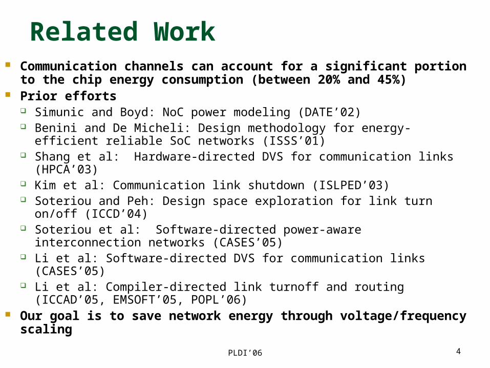
Related Work Communication channels can account for a significant portion to the chip

energy consumption (between 20% and 45%) Prior efforts

Simunic and Boyd: NoC power modeling (DATE’02) Benini and De Micheli: Design methodology for energy-efficient reliable SoC

networks (ISSS’01) Shang et al: Hardware-directed DVS for communication links (HPCA’03) Kim et al: Communication link shutdown (ISLPED’03) Soteriou and Peh: Design space exploration for link turn on/off (ICCD’04) Soteriou et al: Software-directed power-aware interconnection networks

(CASES’05) Li et al: Software-directed DVS for communication links (CASES’05) Li et al: Compiler-directed link turnoff and routing (ICCAD’05, EMSOFT’05,

POPL’06) Our goal is to save network energy through voltage/frequency scaling

PLDI’06 5

Motivational Example (1)

for i = 0 to N { send(2, A[i][0..1023] receive(2, buffer)}

for i = 0 to N{ send(1, A[i][0..255] receive(1, buffer)}

Node 1 Node 2

i=0 i=1 i=2 i=3 i=4

PLDI’06 6

Motivational Example (2)

for i = 0 to N { send(2, A[i][0..255] short computation receive(2, buffer)}

for i = 0 to N{ send(1, A[i][0..255] long computation receive(1, buffer)}

Node 1 Node 2

i=0 i=1 i=2 i=3 i=4

Node 1

Node 2

Node 1

Node 2

PLDI’06 7

Overview of Our Approach

InputParallelCode

IPCG

Scaling Factorfor Each

Connection

OutputParallelCode

BuildingIPCG

CriticalPath

Analysis

CodeModification

•Process and Connection Mapping•NoC Parameters

PLDI’06 8

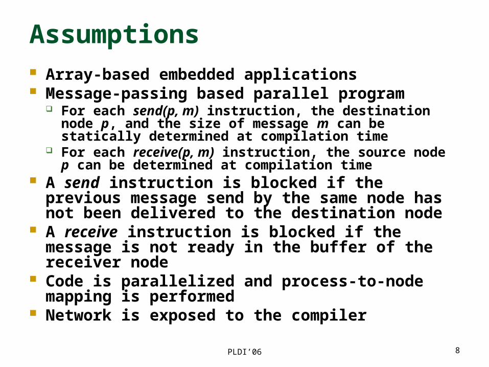
Assumptions Array-based embedded applications Message-passing based parallel program

For each send(p, m) instruction, the destination node p, and the size of message m can be statically determined at compilation time

For each receive(p, m) instruction, the source node p can be determined at compilation time

A send instruction is blocked if the previous message send by the same node has not been delivered to the destination node

A receive instruction is blocked if the message is not ready in the buffer of the receiver node

Code is parallelized and process-to-node mapping is performed

Network is exposed to the compiler

PLDI’06 9

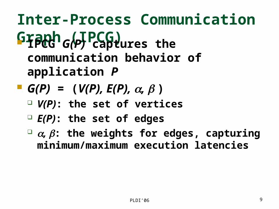
Inter-Process Communication Graph (IPCG) IPCG G(P) captures the communication behavior of

application P G(P) = (V(P), E(P), , )

V(P): the set of vertices E(P): the set of edges , : the weights for edges, capturing minimum/maximum

execution latencies

PLDI’06 10

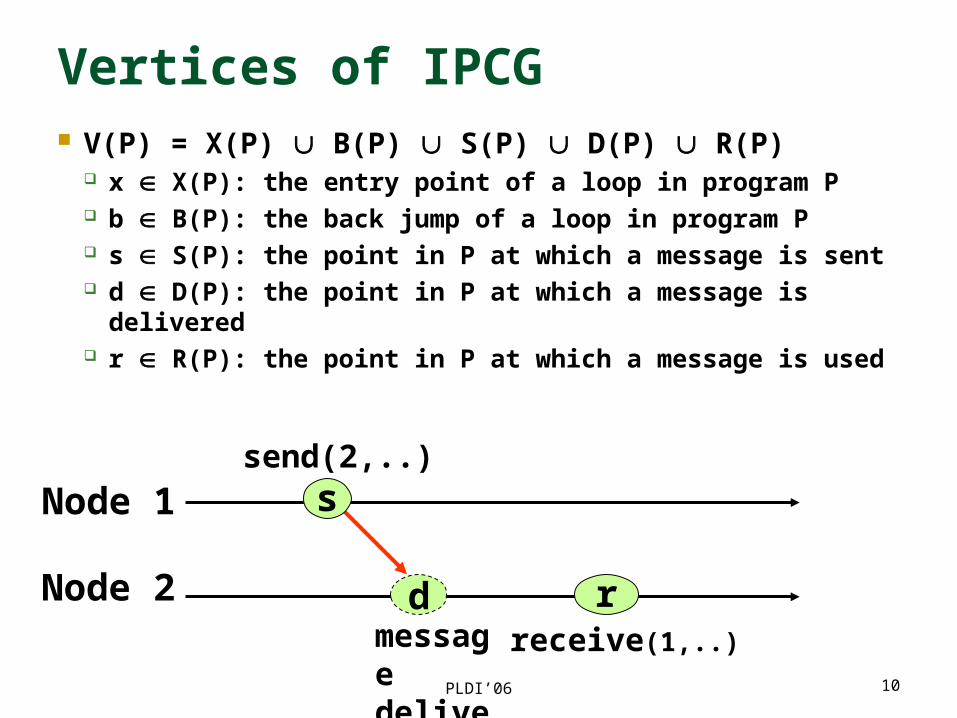
Vertices of IPCG V(P) = X(P) B(P) S(P) D(P) R(P)

x X(P): the entry point of a loop in program P b B(P): the back jump of a loop in program P s S(P): the point in P at which a message is sent d D(P): the point in P at which a message is delivered r R(P): the point in P at which a message is used

Node 1

Node 2

send(2,..)

receive(1,..)

s

d rmessagedelivered

PLDI’06 11

Edges of IPCG Task edges

Communication edge (s, d): a message is sent at point s S(P) and delivered at point d D(P)

Computation edge (u, v): a computation task starts at point u and ends at point v u, v X(P) S(P) R(P)

Control edges Enforce the order at which the points of the given

program can be reached Back-jump edge Other control edges

PLDI’06 12

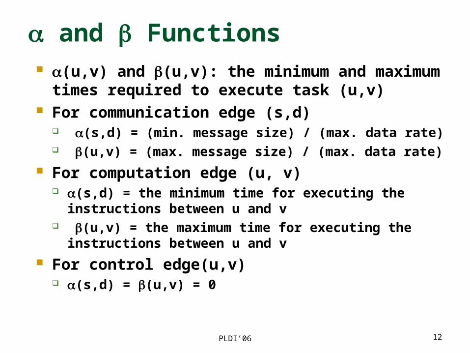
and Functions (u,v) and (u,v): the minimum and maximum times

required to execute task (u,v) For communication edge (s,d)

(s,d) = (min. message size) / (max. data rate) (u,v) = (max. message size) / (max. data rate)

For computation edge (u, v) (s,d) = the minimum time for executing the instructions between

u and v (u,v) = the maximum time for executing the instructions between

u and v For control edge(u,v)

(s,d) = (u,v) = 0

PLDI’06 13

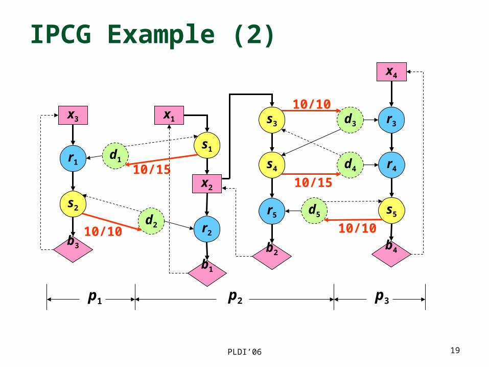
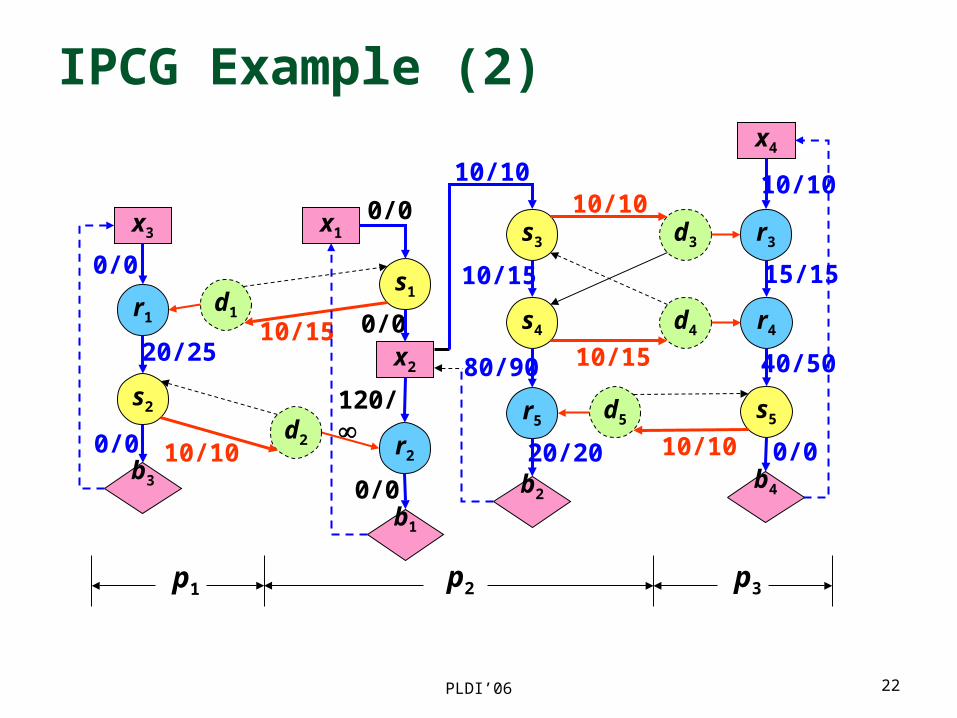
IPCG Example (1)

// Process 1x3:for(...) { r1:receive(2,..) 20–25 cycles s2:send(2,..)}

// Process 2x1:for(...) { s1:send(1,..); x2:for(...) { 10 cycles s3:send(3,..); 10–15 cycles s4:send(3,..); 80-90 cycles r5:receive(3,..) 20 cycles } r2:receive(1,..);}

// Process 3x4:for(...) { 10 cycles r3:receive(2,..) 15 cycles r4:receive(2,..) 40-50 cycles s5:send(2,..)}

PLDI’06 14

IPCG Example (2)

0/0

0/0

0/0

120/

x2

s4

r5

x1

s1

r2

r4

s5

x4

r1

s2

x3

0/0

20/25

0/0

15/15

40/50

0/0

10/10

80/90

20/20

10/15

10/10

10/15

10/10

p1 p2 p3

b3

b1

b2b4

s3 r3

d1

d2

10/15

d3

10/10

d4

d5

10/10

PLDI’06 15

IPCG Example (2)

x2

s4

r5

x1

s1

r2

r4

s5

x4

r1

s2

x3

p1 p2 p3

b3

b1

b2b4

s3 r3

d1

d2

d3

d4

d5

PLDI’06 16

IPCG Example (2)

x2

s4

r5

x1

s1

r2

r4

s5

x4

r1

s2

x3

p1 p2 p3

b3

b1

b2b4

s3 r3

d1

d2

d3

d4

d5

PLDI’06 17

IPCG Example (2)

x2

s4

r5

x1

s1

r2

r4

s5

x4

r1

s2

x3

p1 p2 p3

b3

b1

b2b4

s3 r3

d1

d2

d3

d4

d5

PLDI’06 18

IPCG Example (2)

x2

s4

r5

x1

s1

r2

r4

s5

x4

r1

s2

x3

p1 p2 p3

b3

b1

b2b4

s3 r3

d1

d2

d3

d4

d5

PLDI’06 19

IPCG Example (2)

x2

s4

r5

x1

s1

r2

r4

s5

x4

r1

s2

x3

10/15

10/10

10/15

10/10

p1 p2 p3

b3

b1

b2b4

s3 r3

d1

d2

d3

10/10

d4

d5

PLDI’06 20

IPCG Example (2)

0/0

0/0

0/0

120/

x2

s4

r5

x1

s1

r2

r4

s5

x4

r1

s2

x3

0/0

20/25

0/0

15/15

40/50

0/0

10/10

80/90

20/20

10/15

10/10

10/15

10/10

p1 p2 p3

b3

b1

b2b4

s3 r3

d1

d2

10/15

d3

10/10

d4

d5

10/10

PLDI’06 21

IPCG Example (2)

0/0

0/0

0/0

120/

x2

s4

r5

x1

s1

r2

r4

s5

x4

r1

s2

x3

0/0

20/25

0/0

15/15

40/50

0/0

10/10

80/90

20/20

10/15

10/10

10/15

10/10

p1 p2 p3

b3

b1

b2b4

s3 r3

d1

d2

10/15

d3

10/10

d4

d5

10/10

PLDI’06 22

IPCG Example (2)

0/0

0/0

0/0

120/

x2

s4

r5

x1

s1

r2

r4

s5

x4

r1

s2

x3

0/0

20/25

0/0

15/15

40/50

0/0

10/10

80/90

20/20

10/15

10/10

10/15

10/10

p1 p2 p3

b3

b1

b2b4

s3 r3

d1

d2

10/15

d3

10/10

d4

d5

10/10

PLDI’06 23

IPCG Example (2)

0/0

0/0

0/0

120/

x2

s4

r5

x1

s1

r2

r4

s5

x4

r1

s2

x3

0/0

20/25

0/0

15/15

40/50

0/0

10/10

80/90

20/20

10/15

10/10

10/15

10/10

p1 p2 p3

b3

b1

b2b4

s3 r3

d1

d2

10/15

d3

10/10

d4

d5

10/10

PLDI’06 24

IPCG Example (2)

0/0

0/0

0/0

120/

x2

s4

r5

x1

s1

r2

r4

s5

x4

r1

s2

x3

0/0

20/25

0/0

15/15

40/50

0/0

10/10

80/90

20/20

10/15

10/10

10/15

10/10

p1 p2 p3

b3

b1

b2b4

s3 r3

d1

d2

10/15

d3

10/10

d4

d5

10/10

PLDI’06 25

Parallel Loop Group A set of loops that communicate with each other Unit of granularity for optimization

0/0

0/0

0/0

120/

x2

s4

r5

x1

s1

r2

r4

s5

x4

r1

s2

x3

0/0

20/25

0/0

15/15

40/50

0/0

10/10

80/90

20/20

10/15

10/10

10/15

10/10b3

b1

b2b4

s3 r3

d1

d2

10/15

d3

10/10

d4

d5

10/10

PLDI’06 26

Representative Iterations A set of loop iterations that represent the timing

behavior of the entire parallel loop group

T T

t1,0

t2,0

t3,0

t4,0

j = 0t1,1

t2,1

t3,1

t4,1

j = 1t1,2

t2,2

t3,2

t4,2

j = 2t1,3

t2,3

t3,3

t4,3

j = 3t1,4

t2,4

t3,4

t4,4

j = 4t1,5

t2,5

t3,5

t4,5

j = 5t1,6

t2,6

t3,6

t4,6

j = 6t1,7

t2,7

t3,7

t4,7

j = 7t1,8

t2,8

t3,8

t4,8

j = 8

Time

Loop x1

Loop x2

Loop x3

Loop x4

q = 1 Q = 4

R = 3 Tttqj Rjiji ,,: Tttqj Rjiji ,,:

PLDI’06 27

Critical Path Analysis Determine q and Q such that [q, Q – 1] are the set of

representative loop iterations Determine t[i,j]: the earliest time that node vi at the jth

iteration (j [q, Q-1]) can be reached, assuming each task is completed in the shortest time

Determine t[i,j]: the earliest time that node vi at the jth iteration (j [q, Q-1]) can be reached, assuming each task takes the longest time

Determine the scaling factor for each communication channel such that the overall performance degradation due to voltage scaling is within (a preset bound)

PLDI’06 28

Determining t[i,j] - Constraints

]1,[],[:),(

),(],[],[:),(

0]0,[:

jktjitEik

ikjktjitEik

iti

whereQj 0

E

E

: the set of intra-iteration edges

: the set of inter-iteration edges

Evu ),( : at each iteration j, u must be reached before v

Evu ),( : u at the (j – 1)th iteration must be reached before v at the jth iteration

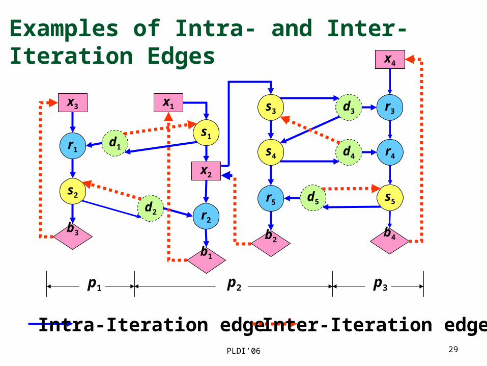
PLDI’06 29

Examples of Intra- and Inter-Iteration Edges

x2

s4

r5

x1

s1

r2

r4

s5

x4

r1

s2

x3

p1 p2 p3

b3

b1

b2b4

s3 r3

d1

d2

d3

d4

d5

Intra-Iteration edge Inter-Iteration edge

PLDI’06 30

Determining t[i,j] - Example

20/2520/2520/25

s1

r1

x1

20/25

10/10b1

s2

r2

x2

25/30

25/30b2

s3

r3

x3

20/20

15/15b3

p1 p2 p3

d1 d1 d3

PLDI’06 31


x1 s1 d1 r1 b1 x2 s2 d2 r2 b2 x3 s3 d3 r3 b3

t[i,0] 0 0 0 0 0 0 0 0 0 0 0 0 0 0 0

t[s1,0] + (s1, d1) t[d1, 0] 0 + 20 = 20

20

PLDI’06 32



t[i,0] 0 0 20 20 30 0 0 20 25 50 0 0 20 20 35

t[i,1] 30 20 0 0 0 20 50 0 0 0 35 20 0 0 0

PLDI’06 33



t[i,0] 0 0 20 20 30 0 0 20 25 50 0 0 20 20 35

t[i,1] 30 30 50 55 65 50 50 70 75 100 35 35 55 70 85

PLDI’06 34

Determining t[i,j] – Example


t[i,0] 0 0 20 20 30 0 0 20 25 50 0 0 20 20 35

t[i,1] 30 30 50 55 65 50 50 70 75 100 35 35 55 70 85

t[i,2] 65 65 85 105 115 100 100 120 125 150 85 85 105 120 135

t[i,3] 115 115 135 155 165 150 150 170 175 200 135 135 155 170 185

t[i,4] 165 .... .... .... .... 200 .... .... .... .... 185 .... .... .... ....

q = 2, Q = 4, T = 50q = 2, Q = 4, T = 50

PLDI’06 35

Determining t[i,j] - Constraints

]1,[],[:),(

),(],[],[:),(

],[],[:

jktjitEik

ikjktjitEik

qitqiti

whereQj 0

EE

: the set of intra-iteration edges

: the set of inter-iteration edges

PLDI’06 36

Determining Scaling Factor -Constraints

]},[],[,)1max{(],[],[:

]1,[],[:),(

)](),([/),(],[],[:),(

],[],[:

qitQitTqitQiti

jktjitEik

vvkikjktjitEik

qitqiti

ik

where Qj 0 EE , : the set of intra-iteration and inter-iteration edges)(v : the node that executes operation v

),( 21 nnk : the scaling factor for the network connection from node n1 to n2

We try to maximize k(n1, n2) for each connection

1),(0 21 nn

: the maximum performance degradation allowed

PLDI’06 37

Determining Scaling Factor - Algorithmrepeat

select a connection Cscale down the data rate of C by one gradedetermine t[i, j] using

if make the data rate of C permanent

else restore the data rate of C

until no more connection can be scale down

]1,[],[:),(

)](),([/),(],[],[:),(

],[],[:

jktjitEik

vvkikjktjitEik

qitqiti

ik

]},[],[,)1max{(],[],[: qitQitTqitQiti

PLDI’06 38

Determining Scaling Factor - Example


t[i,q] 65 65 85 105 115 100 100 120 125 150 85 85 105 120 135

t[i,Q] 165 .... .... .... .... 200 .... .... .... .... 185 .... .... .... ....

t[i,Q] 170 .... .... .... .... 210 .... .... .... .... 190 .... .... .... ....

tmax[i,Q] 175 .... .... .... .... 210 .... .... .... .... 195 .... .... .... ....

q = 2, Q = 4, T = 100, = 10%, k = 1, 0.8, 0.6, 0.4, 0.2

PLDI’06 39



t[i,q] 65 65 85 105 115 100 100 120 125 150 85 85 105 120 135

t[i,Q] 165 .... .... .... .... 200 .... .... .... .... 185 .... .... .... ....

t[i,Q] 170 .... .... .... .... 210 .... .... .... .... 190 .... .... .... ....

tmax[i,Q] 175 .... .... .... .... 210 .... .... .... .... 195 .... .... .... ....

q = 2, Q = 4, T = 100, = 10%, k = 1, 0.8, 0.6, 0.4, 0.2

k[1, 2] = 0.8, k[2, 3] = 1, k[3, 1] = 1


t[i,Q] 170 .... .... .... .... 210 .... .... .... .... 190 .... .... .... ....

PLDI’06 40



t[i,q] 65 65 85 105 115 100 100 120 125 150 85 85 105 120 135

t[i,Q] 165 .... .... .... .... 200 .... .... .... .... 185 .... .... .... ....

t[i,Q] 170 .... .... .... .... 210 .... .... .... .... 190 .... .... .... ....

tmax[i,Q] 175 .... .... .... .... 210 .... .... .... .... 195 .... .... .... ....

q = 2, Q = 4, T = 100, = 10%, k = 1, 0.8, 0.6, 0.4, 0.2

k[1, 2] = 0.8, k[2, 3] = 0.8, k[3, 1] = 1


t[i,Q] 170 .... .... .... .... 210 .... .... .... .... 196.25 .... .... .... ....

PLDI’06 41



t[i,q] 65 65 85 105 115 100 100 120 125 150 85 85 105 120 135

t[i,Q] 165 .... .... .... .... 200 .... .... .... .... 185 .... .... .... ....

t[i,Q] 170 .... .... .... .... 210 .... .... .... .... 190 .... .... .... ....

tmax[i,Q] 175 .... .... .... .... 210 .... .... .... .... 195 .... .... .... ....

q = 2, Q = 4, T = 100, = 10%, k = 1, 0.8, 0.6, 0.4, 0.2

k[1, 2] = 0.8, k[2, 3] = 1, k[3, 1] = 0.8


t[i,Q] 176.25 .... .... .... .... 210 .... .... .... .... 190 .... .... .... ....

PLDI’06 42



t[i,q] 65 65 85 105 115 100 100 120 125 150 85 85 105 120 135

t[i,Q] 165 .... .... .... .... 200 .... .... .... .... 185 .... .... .... ....

t[i,Q] 170 .... .... .... .... 210 .... .... .... .... 190 .... .... .... ....

tmax[i,Q] 175 .... .... .... .... 210 .... .... .... .... 195 .... .... .... ....

q = 2, Q = 4, T = 100, = 10%, k = 1, 0.8, 0.6, 0.4, 0.2

k[1, 2] = 0.6, k[2, 3] = 1, k[3, 1] = 1


t[i,Q] 170 .... .... .... .... 210 .... .... .... .... 190 .... .... .... ....

PLDI’06 43



t[i,q] 65 65 85 105 115 100 100 120 125 150 85 85 105 120 135

t[i,Q] 165 .... .... .... .... 200 .... .... .... .... 185 .... .... .... ....

t[i,Q] 170 .... .... .... .... 210 .... .... .... .... 190 .... .... .... ....

tmax[i,Q] 175 .... .... .... .... 210 .... .... .... .... 195 .... .... .... ....

q = 2, Q = 4, T = 100, = 10%, k = 1, 0.8, 0.6, 0.4, 0.2

k[1, 2] = 0.4, k[2, 3] = 1, k[3, 1] = 1


t[i,Q] 170 .... .... .... .... 210 .... .... .... .... 190 .... .... .... ....

PLDI’06 44



t[i,q] 65 65 85 105 115 100 100 120 125 150 85 85 105 120 135

t[i,Q] 165 .... .... .... .... 200 .... .... .... .... 185 .... .... .... ....

t[i,Q] 170 .... .... .... .... 210 .... .... .... .... 190 .... .... .... ....

tmax[i,Q] 175 .... .... .... .... 210 .... .... .... .... 195 .... .... .... ....

q = 2, Q = 4, T = 100, = 10%, k = 1, 0.8, 0.6, 0.4, 0.2

k[1, 2] = 0.2, k[2, 3] = 1, k[3, 1] = 1


t[i,Q] 170 .... .... .... .... 210 .... .... .... .... 190 .... .... .... ....

PLDI’06 45



t[i,q] 65 65 85 105 115 100 100 120 125 150 85 85 105 120 135

t[i,Q] 165 .... .... .... .... 200 .... .... .... .... 185 .... .... .... ....

t[i,Q] 170 .... .... .... .... 210 .... .... .... .... 190 .... .... .... ....

tmax[i,Q] 175 .... .... .... .... 210 .... .... .... .... 195 .... .... .... ....

q = 2, Q = 4, T = 100, = 10%, k = 1, 0.8, 0.6, 0.4, 0.2

k[1, 2] = 0.2, k[2, 3] = 1, k[3, 1] = 1


t[i,Q] 170 .... .... .... .... 270 .... .... .... .... 190 .... .... .... ....

RESULT: k[1, 2] = 0.4, k[2, 3] = 1, k[3, 1] = 1

PLDI’06 46

Shared Communication Channels

The voltage level of the channel shared by multiple connections is determined by the connection that requires the highest voltage level

a c

b b

c a

]]',[[and]]',[[ sconnectionby shared bbaa

]]',[[and]]',[[ sconnectionby shared ccaa

v1

v1

v2

v3

v2 v2

v3

v3

v1

v1

PLDI’06 48

Experimental Setup

Parameter Value

NoC topology 5 * 5 mesh

Idle channel power 8.6pJ/cycle

Voltage switch energy 1020pJ,

Voltage delay 120 cycles

Processor 1GHz, 2-issue

Node local memory 20KB

Package header size 3 flits

Flit size 39bits

Voltage

(V)

Rate

(bps)

Energy

(pJ/bit)

0.7 200M 4.21

0.9 660M 5.25

1.1 1.33G 6.49

1.3 1.93G 8.31

1.5 2.50G 10.21

PLDI’06 49

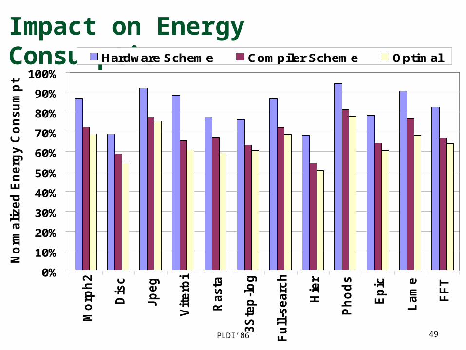
Impact on Energy Consumption

0%

10%

20%

30%

40%

50%

60%

70%

80%

90%

100%M

orp

h2

Dis

c

Jp

eg

Vit

erb

i

Rasta

3S

tep

-lo

g

Fu

ll-s

earc

h

Hie

r

Ph

od

s

Ep

ic

Lam

e

FF

T

No

rmali

zed

En

erg

y C

on

su

mp

tio

n

Hardware Scheme Compiler Scheme Optimal

PLDI’06 50

Energy Consumption Breakdown

0%

10%

20%

30%

40%

50%

60%

70%

80%

90%

100%

Mo

rph

2

Dis

c

Jp

eg

Vit

erb

i

Rasta

3S

tep

-lo

g

Fu

ll-s

earc

h

Hie

r

Ph

od

s

Ep

ic

Lam

e

FF

T

En

erg

y B

reakd

ow

n

1.5V 1.3V 1.1V 0.9V 0.7V overhead

PLDI’06 51

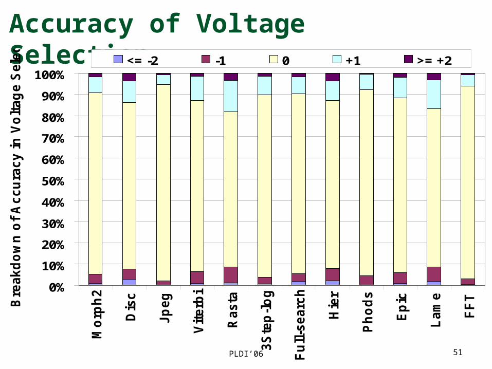
Accuracy of Voltage Selection

0%

10%

20%

30%

40%

50%

60%

70%

80%

90%

100%

Mo

rph

2

Dis

c

Jp

eg

Vit

erb

i

Rasta

3S

tep

-lo

g

Fu

ll-s

earc

h

Hie

r

Ph

od

s

Ep

ic

Lam

e

FF

TBre

akd

ow

n o

f A

ccu

racy i

n V

olt

ag

e S

ele

cti

on

<= -2 -1 0 +1 >= +2

PLDI’06 52

Conclusions and Research Directions

NoC presents unique opportunities for compilers Expose network layout to compiler for energy reduction

through voltage scaling and channel shutdown We implemented a compiler directed voltage

scaling algorithm and compared its performance to a hardware scheme Promising results

Research Directions Evaluating impact of process-to-node mapping Combined voltage/frequency scaling for NoC and CPUs Metrics other than energy (e.g., temperature, reliability,

…)

Thank you!http://www.cse.psu.edu/~mdl

[email protected]

Funded in part byGSRC and NSF

reducing noc energy consumption through compiler-directed channel voltage scaling guangyu chen,...

Documents

node mapping

destination node p

compiler slide

receiver node code

source node p

voltagefrequency scaling

vertices of ipcg vp

noc energy consumption