Redif, Soydan and Weiss, Stephan and McWhirter, John G. (2017)

Relevance of polynomial matrix decompositions to broadband blind

signal separation. Signal Processing, 134. pp. 76-86. ISSN 0165-1684 ,

http://dx.doi.org/10.1016/j.sigpro.2016.11.019

This version is available at https://strathprints.strath.ac.uk/59776/

Strathprints is designed to allow users to access the research output of the University of

Strathclyde. Unless otherwise explicitly stated on the manuscript, Copyright © and Moral Rights

for the papers on this site are retained by the individual authors and/or other copyright owners.

Please check the manuscript for details of any other licences that may have been applied. You

may not engage in further distribution of the material for any profitmaking activities or any

commercial gain. You may freely distribute both the url (https://strathprints.strath.ac.uk/) and the

content of this paper for research or private study, educational, or not-for-profit purposes without

prior permission or charge.

Any correspondence concerning this service should be sent to the Strathprints administrator:

strathprints@strath.ac.uk

The Strathprints institutional repository (https://strathprints.strath.ac.uk) is a digital archive of University of Strathclyde research

outputs. It has been developed to disseminate open access research outputs, expose data about those outputs, and enable the

management and persistent access to Strathclyde's intellectual output.

Contents lists available at ScienceDirect

Signal Processing

journal homepage: www.elsevier.com/locate/sigpro

Review

Relevance of polynomial matrix decompositions to broadband blind signal

separation

Soydan Redifa,⁎

, Stephan Weissb,1, John G. McWhirterc

a Department of Electrical & Electronic Engineering, European University of Lefke, Lefke, North Cyprusb Department of Electronic & Electrical Engineering, University of Strathclyde, Glasgow G11XW, Scotlandc Cardiff University, Cardiff CF24 3AA, Wales, UK

A R T I C L E I N F O

Keywords:

Paraunitary matrix

Parahermitian matrix

Polynomial matrix eigenvalue decomposition

Broadband blind signal separation

Broadband adaptive beamforming

Radar

Sonar

A B S T R A C T

The polynomial matrix EVD (PEVD) is an extension of the conventional eigenvalue decomposition (EVD) to

polynomial matrices. The purpose of this article is to provide a review of the theoretical foundations of the

PEVD and to highlight practical applications in the area of broadband blind source separation (BSS). Based on

basic definitions of polynomial matrix terminology such as parahermitian and paraunitary matrices, strong

decorrelation and spectral majorisation, the PEVD and its theoretical foundations will be briefly outlined. The

paper then focuses on the applicability of the PEVD and broadband subspace techniques — enabled by the

diagonalisation and spectral majorisation capabilities of PEVD algorithms — to define broadband BSS solutions

that generalise well-known narrowband techniques based on the EVD. This is achieved through the analysis of

new results from three exemplar broadband BSS applications — underwater acoustics, radar clutter

suppression, and domain-weighted broadband beamforming — and their comparison with classical broadband

methods.

1. Introduction

Over the last decade, algorithms that extend the eigenvalue

decomposition (EVD) to the realm of polynomial matrices have had a

growing impact on signal processing theory and practice, mainly

because they can be used to solve generalisations of narrowband

problems typically addressed by the EVD, including subspace decom-

position. The extension of EVD to parahermitian (PH) polynomial

matrices, referred to as polynomial matrix EVD (PEVD), gives an

immediate broadband generalisation of the concepts of signal and

noise subspaces, and hence subspace decompositions. Just as principal

component analysis (PCA) based on the EVD is fundamental to most

narrowband BSS formulations, the PEVD can be a powerful tool for

broadband or convolutive blind source separation (BSS).

The classical approach to narrowband BSS begins by exploiting

second-order statistics to generate uncorrelated sequences from nar-

rowband, instantaneously mixed signals by performing principal

component analysis (PCA) [1,2]. PCA is usually obtained through

matrix factorisation by means of a unitary matrix decomposition, such

as the singular value (SVD) or eigenvalue decomposition (EVD) [3,4].

To complete the BSS process, a “hidden” rotation matrix is determined

via on higher-order statistics (HOS), which permutes entries to achieve

spectral coherence across frequency bins. With little or no prior

knowledge and minimal assumptions, a BSS method can often be used

to extract a wanted signal from among interference signals. However,

the wanted signal is in no way accentuated by these underlying

assumptions.

Incorporation of a priori knowledge of the signals into the BSS

problem can be formulated in the framework of signal decompositions

and matrix factorisations, and address statistical dependence, periodi-

city, spectral shape, time coherence or smoothness [5–8]. The goal

often is to estimate a reduced coordinate space, which provides a more

accurate physical representation of the sources or mixing parameters.

The above signal decompositions are based on an instantaneous

mixing model, where the propagation of signals from sources to the

array is modelled as a scalar mixing matrix. However, in many

important applications such as broadband array processing, convolu-

tive mixing — or a matrix of finite impulse response (FIR) filters —

must be used instead. The transfer function of such a matrix of FIR

filters forms a polynomial matrix, which can accurately model effects

such as multipath propagation, or the lag-dependent correlation

between different broadband sensor signals. SVD- or EVD-based

decompositions generally can only decorrelate instantaneously, i.e.,

only for zero lag. Following convolutive mixing, strong decorrelation

http://dx.doi.org/10.1016/j.sigpro.2016.11.019

Received 26 May 2016; Received in revised form 7 October 2016; Accepted 24 November 2016

⁎ Corresponding author.

1 EURASIP Member.

E-mail addresses: sredif@eul.edu.tr (S. Redif), stephan.weiss@strath.ac.uk (S. Weiss), mcwhirterjg@cardiff.ac.uk (J.G. McWhirter).

Signal Processing 134 (2017) 76–86

Available online 25 November 2016

0165-1684/ © 2016 Elsevier B.V. All rights reserved.

MARK

[9] eliminates correlation for all lag values, and can be achieved using a

well-designed matrix of FIR filters.

In the past, broadband BSS has been addressed by performing

narrowband BSS at each frequency bin simultaneously, through

application of the discrete Fourier transform (DFT) — commonly

referred to as independent frequency bin (IFB) processing. However,

coherence restoration is required after BSS via permutation matrices

applied in every bin [10,11]. An alternative is to adopt coherent signal

subspace-related methods, which generally require some prior knowl-

edge of signals, such as direction and fractional bandwidth, to

coherently combine covariance matrices across different bins in order

to create an approximately narrowband problem [12–14].

The formulation and decomposition of polynomial matrices pre-

sents an alternative to these classical broadband BSS approaches.

Polynomial matrices have been used for many years, e.g., in the area of

control [15] or broadband subspace decomposition and adaptive

sensor arrays [16–18]. Various polynomial matrix factorisations have

been addressed, such as the Smith–Macmillan form [19], or poly-

nomial matrix factors that are paraunitary (PU) or lossless [20–33].

Typically, the filter is chosen to optimise a specific objective function

for a known input power spectral density (PSD), such as coding gain

[9,20,23,31,32] for subband coding.

The space–time covariance matrix derived from broadband sensor

data includes auto- and cross-correlation terms, whose symmetries

create the specific form of a parahermitian (PH) polynomial matrix.

The PEVD of such a PH matrix was proposed in [16,25,26], and leads

to a factorisation where a diagonal PH matrix containing the poly-

nomial eigenvalues is pre- and post-multiplied by a PU matrix, or

lossless, filter bank. The existence of such a factorisation based on FIR

PU matrices is not ascertained [19], but suggested that it exists at least

in good approximation [34].

The polynomial eigenvalues of a PEVD represent the power spectral

densities of the strongly decorrelated signals. Depending on the PEVD

algorithm (discussed below), the eigenvalues can be ordered akin to the

singular values of the SVD at every frequency. The ordering of the

spectra in this way is called spectral majorisation [9,26], and is useful

in a number of applications.

An initial iterative scheme to approximate the PEVD, the second

order sequential best rotation (SBR2) algorithm [26], has triggered

similar or related efforts [28–33,35–40]. SBR2 has been proven to

converge [26,31], and found to approximate the ideal PEVD very

closely [34]. A coding-gain based version of SBR2 (SBR2C) was shown

to offer improved convergence in [31].

More recently, the sequential matrix decomposition (SMD) and

maximum-element (ME-SMD) algorithms [33] have shown superior

convergence due to their advanced energy transfer ability, as compared

to other iterative algorithms. The multiple-shift variant of the ME-SMD

in [36] has shown marked improvement in convergence speed com-

pared to SMD.

The SMD and SBR2 algorithms have been successfully applied to a

number of broadband extensions of narrowband problems, tradition-

ally addressed by the EVD, including, e.g., broadband array processing

[41–47], channel coding [48], broadband communications [49], spec-

tral factorisation [50], convolutive BSS [42,46], and the design of FIR

PU filter banks for subband coding [31,32]. The recent parallelisation

of SBR2 in [35], for field programmable gate arrays, has enabled

application of SBR2 to real-time problems using embedded processing

[51].

The advantage of polynomial matrix decompositions over IFB

processing lies in the natural ability of broadband decomposition

algorithms to preserve and exploit the coherence of signals.

As a particular example of applying the PEVD to convolutive BSS

with prior knowledge, in [42] a broadband extension to the narrow-

band semi-blind signal approach in [52] has been performed. The

broadband equivalent method used some prior information about the

direction of sources acquired by a broadband array was embedded to

achieve an enhanced separation of sources. This can be combined with

other broadband approaches, such as polynomial MUSIC [44,45], to

estimate the prior knowledge that can then be passed to the BSS

problem.

The aim of this paper is twofold: (i) provide an overview of

polynomial matrix factorisation and (ii) discuss applications in the

area of broadband BSS. In Section 2, the PEVD and related funda-

mental concepts, such as paraunitarity, strong decorrelation and

spectral majorisation, are introduced. In Sections 3 and 4, we present

solutions and new results to three important problems via a PEVD-

based broadband beamformer and domain-weighted PEVD. The re-

sults are compared to classical methods, which contrast the natural

ability of broadband subspace decomposition algorithms to preserve

and exploit the coherence of signals. Lastly, conclusions are drawn in

Section 5.

2. Polynomial matrix eigenvalue decomposition

2.1. Notation

In this paper matrices and vectors are represented by bold upper-

case and bold lowercase characters, e.g., X and x, respectively. An

element of X is denoted by xjk. Complex conjugation, matrix transposi-

tion and Hermitian transposition are indicated by the superscripts *, T

and H, respectively. A p p× (complex-valued) Hermitian matrixR ∈ p p× has the property R R= H; a unitary matrix U ∈ p p× has the

property U U UU I= = pH H , where Ip is the p p× identity matrix.

Polynomial matrices are polynomials with matrix-valued coeffi-

cients, or matrices with polynomial elements [15,19]. An n q× poly-

nomial matrix in the indeterminate variable z−1 is denoted by

∑A z τ zA( ) = [ ] ,τ t

t

τ

=

−

1

2

(1)

where a z a τ z( ) = ∑ [ ]ij τ t

tij

τ=

−1

2 , t t≤1 2, τ ∈ and a τ[ ] ∈ij , is an element

of τA[ ]. Hence, coefficient matrices of A z( ) can be written as

t tA A[ ],…, [ ]1 2 ; e.g., the coefficient matrix of lag zero (lag-zero coefficient

matrix) is denoted A[0]. Note that the effective order of A z( ) is t t−2 1. A

transform pair as in (1) is abbreviated as A z τA( ) •—∘ [ ]. Also note that

parentheses express dependency on continuous variables, while square

brackets denote dependency on discrete variables.

2.2. Space–time covariance matrix

It is well-known that instantaneous spatial correlation, i.e., correla-

tion between pairs of signals sampled at the same instant in time, can

be removed using the EVD and SVD [4]. Therefore, the SVD (or EVD)

can be used to decorrelate instantaneous mixtures, e.g., for the case of

narrowband sensor arrays. However, convolutively mixed signals, or

signals derived from a broadband sensor array, cannot be decorrelated

in this way. The sensor-weight values required to correct for the time

delay between sensors are different for different frequencies. Frequency

dependent weights can be realised using FIR filters, which form a

frequency dependent response for each sensor signal in order to

compensate the phase difference for the different frequency compo-

nents. The sensors thus sample the propagating wave field in both

space and time.

Hence, in order to express the signals at the sensors, we modify the

well-known instantaneous-mixing (or narrowband) model to take

account of this process

ηt t t tx A s[ ] = [ ]* [ ] + [ ], (2)

where the asterisk denotes multi-input multi-output (MIMO) convolu-

tion [51], Aτ zA[ ]∘—• ( ) is the p q× mixing matrix of FIR filters a t[ ]ij

and ts[ ] ∈ q and η t[ ] represent independent source and noise signals.

The signals tx[ ] will generally be correlated over multiple time lags,

S. Redif et al. Signal Processing 134 (2017) 76–86

77

so that the space–time covariance matrix,

τ t t τR x x[ ] = { [ ] [ − ]} ∈ ,p pH × (3)

will generally not be diagonal for all τ, where {·} denotes the

expectation operator. It follows that the cross-spectral density (CSD)

matrix, R z τR( ) •—○ [ ], will also not be diagonal. It can be shown that

the CSD matrices of the signal and noise sources are both diagonal

because of the independence assumption.

The matrix R z eR( ) | = ( ) ∈z ejΩ p p

=×

jΩ is Hermitian for all normal-

ised frequencies Ω. Equivalently, we say that the polynomial matrix is

parahermitian (PH): R Rz z z( ) = ( ) ∀∼

, where R z( )∼

is the paraconjugate

of R z( ), i.e., R Rz z( ) = * ( )∼ T −1 , and the asterisk denotes complex conjuga-

tion of the polynomial coefficients. Note that in the case where R z( ) isof order zero, paraconjugation becomes Hermitian conjugate.

2.3. Polynomial eigenvalues and eigenvectors

In order to decompose the space–time covariance matrix τR[ ] of (3)in an analogous fashion to the EVD, the role of the EVD unitary matrix

[3,4] must be generalised to the polynomial case. To this end, we

require a matrix of filters that are lossless: the total power at every

frequency is invariant under the transformation. In linear system

theory, this type of system is termed a lossless (all-pass) MIMO system

[19]. In terms of polynomial matrices, we need a polynomial matrix to

be paraunitary (PU). A polynomial matrix is PU iffH H H Hz z z z I( ) ( ) = ( ) ( ) =

p. Equivalently, H z eH( ) | = ( ) ∈z ejΩ p p

=×

jΩ

is unitary Ω∀ , which is clearly energy preserving.

For PU matrices H z( ) comprising FIR components, the CSD matrix

R z( ) can be decomposed as

H R Hz z z z σ z σ z σ zΣ( ) ≈ ( ) ( ) ( ) = diag{ ( ), ( )… ( )},p1 2 (4)

where σ z σ τ v t v t τ( ) •—∘ [ ] = { [ ] *[ − ]}i i i i are the polynomial eigenva-

lues of R z( ) and the row of H z( ) are the “polynomial eigenvectors” of

R z( ). Here v t[ ]i denote the signals after transformation by H z( ).We use the approximation sign in (4) to indicate that a PEVD

factorisation with FIR PU matrices does not necessarily exist; however,

Icart and Comon have shown that a very close approximation is

possible with arbitrarily large filter orders [34].

The decomposition in (4) represents a generalisation of the EVD to

polynomial matrices, namely polynomial matrix EVD (or PEVD). Note

that (4) becomes the EVD of a Hermitian matrix for a zero-order R z( ).The notion of a unitary matrix for scalar matrices is extended to that of

a PU matrix.

2.4. Strong decorrelation and spectral majorisation

A set of signals v t[ ]i has the strong (total) decorrelation property if

the signals are decorrelated for all relative time delays — not just at the

same time instant for all signals. That is,

v t v t τ{ [ ] [ − ]} = 0,i j (5)

for all t τ, and i j≠ [9]. If the diagonalising PU matrix τH[ ] of (4) is

applied to the signals tx[ ] in (2), i.e.,

t t tv H x[ ] = [ ]* [ ], (6)

then the transformed signals will be strongly decorrelated. In other

words, if H z( ) diagonalises the PH matrix R z( ), it will also impose

strong decorrelation.

The problem of finding a PU matrix with the aim of imposing strong

decorrelation occurs in many other applications besides convolutive

BSS, such as in the design of filter banks for subband coding [9,31,32].

The PU matrix H z( ) in (4) can be designed such that the set of

power spectra σ e{ ( )}ijΩ , where σ e σ z( ) = ( )|i

jΩi z e= jΩ, of the transformed

signals v z( ) satisfies spectral majorisation [9]:

σ e σ e σ e Ω π π( ) ≥ ( ) ≥ ⋯ ≥ ( ), ∀ ∈ [− , ).jΩ jΩp

jΩ1 2 (7)

Note that (7) is the polynomial analogue to an ordered EVD [3] or the

way singular values are ordered by the SVD.

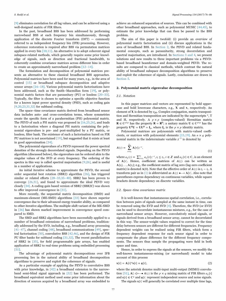
As an example of spectral majorisation via a PU matrix, consider

the power spectra, γ e( )ijΩ , for three arbitrary signals, shown in Fig. 1(a).

These signals clearly do not satisfy the spectral majorisation property

in (7). However, processing these signals with an appropriately

designed PU matrix yields the spectrally majorised PSDs, σ e( )ijΩ , as

shown in Fig. 1(b).

In addition, a PU matrix H z( ) can be found so that the transformed

signals satisfy energy compaction: σ σ[0] ≥ [0]i i+1 , where

σ v t[0] = {| [ ]| }i i2 . Thus, the total spectral power in the first trans-

formed signal v z( )1 is maximised, and the total spectral power in each

of the remaining signals is maximised successively. This property

implies spectral majorisation (in (7)), and is directly analogous to the

singular value ordering for the narrowband case.

Spectral majorisation is a very important property in applications

such as broadband beamforming and BSS. This is because spectrally

majorised signals tend to have most of the related (correlated) signal

energy focused in as few channels as possible [26,41]. This property is

very useful when the aim is to identify the signal subspace, as in

broadband subspace decomposition.

In Sections 3 and 4, we show how the spectral majorisation and

energy compaction properties are of paramount importance in achiev-

ing broadband BSS for signals derived from sensor arrays.

It can be shown that the total input signal power, for all frequencies,

is invariant under a PU transformation [19]. A PU operation cannot

attenuate or amplify the power across channels, it can only redistribute

it, thus maintaining the physical significance of the power of output

signals.

2.5. Approximating the PEVD

All PEVD algorithms presented in the literature to date are

suboptimal since they can only approximate the PEVD. They can also

be viewed as blind methods in the sense that they use minimal a priori

information about the signal sources. The only information used by

these algorithms is the space–time covariance matrix τR[ ] in (3),

which, in practice, is estimated using a finite window of N samples of

the input signal tx[ ]. The accuracy of this estimate is therefore crucial

for the accuracy of the PEVD. Assuming zero-mean signals, an estimate

of the space–time covariance matrix in (3) is given by

Fig. 1. Example of spectral majorisation: signal spectra that (a) do not have and (b) have

the spectral majorisation property.

S. Redif et al. Signal Processing 134 (2017) 76–86

78

∑τN

t τ tR x x[ ] ≜1

[ ] [ − ]t

N

=0

−1H

(8)

and

∑R z τ zR( ) ≜ [ ]τ W

W

τ

=−

−

(9)

is the estimated CSD matrix.

It is assumed that τR[ ] ≅ 0 for τ W| | > [26]; for broadband signals, τR[ ] is negligibly small, if τ| | is large compared to the coherence time. In

practice, W is often measured experimentally. We also assume that

tx[ ] = 0 for values of t outside the sample interval. It can be shown that

the polynomial matrix R z( ) is PH by construction.

Iterative PEVD algorithms such as those of the SBR2 [25,26,31,37]

and SMD families [33,36] may be used to find a PU matrix H z( ) suchthat

H R H Dz z z z( ) ( ) ( ) = ( ), (10)

where D z( ) is approximately diagonal; more specifically,

D z d z d z d z( ) ≈ diag{ ( ), ( )… ( )},p1 2 (11)

where d z d τ v t v t τ( ) •—∘ [ ] ≅ { [ ] *[ − ]}i i i i . The lossless FIR filter H z( )then produces an output tv[ ] according to (6). It can be shown that, to a

good approximation, the signals tv[ ] are strongly decorrelated.

In Sections 3.3 and 4, we demonstrate, via simulation results, the

effectiveness of suboptimal PEVD algorithms as a solution to broad-

band BSS.

3. Broadband BSS using second-order statistics

Consider the problem of recovering a broadband desired signal by a

sensor array in the presence of a broadband interference signal and

noise, as illustrated for the two-sources, two-sensors case in Fig. 2. The

received broadband signals, tx[ ], may be described as convolutive

mixtures of the source signals, ts[ ], as in (2).

A broadband beamformer can be used to steer the beam created by

a sensor array toward the desired signal. Range-bearing plots can then

be produced using the beamformer output, from which the target's

location can be gathered.

3.1. Broadband conventional beamforming

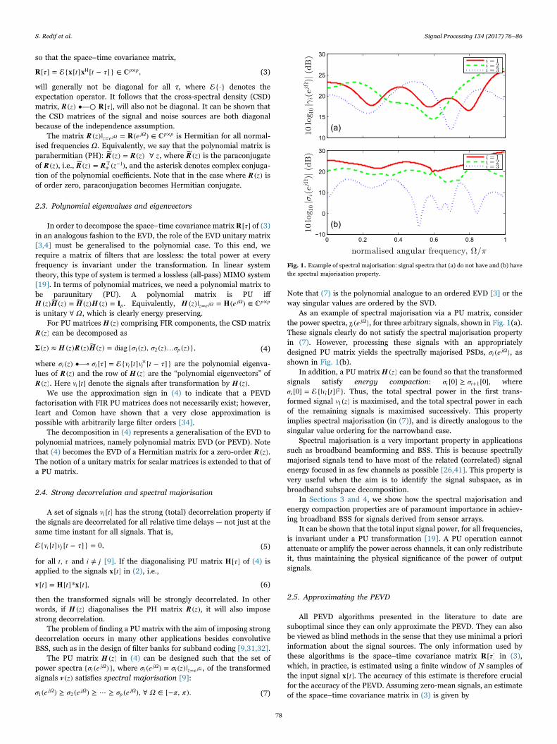
The broadband conventional beamformer (CBF) or tapped delay

line (TDL) beamformer is designed to use prior knowledge to bring the

desired signal to broadside. A block diagram of the broadband CBF is

shown in Fig. 3. Prior information about the direction-of-arrival (DoA)

of the desired signal and the sensor array is used to specify an estimate

of the required pre-steering for the desired signal.

The pre-steering can be expressed as a polynomial vector, a z( )s , and

is an estimate of the true pre-steering polynomial vector. The required

pre-steering can be found by computing the paraconjugate of the sth

column vector in A z( ) of (2), i.e., a z( )∼s . The vector a z( )s describes the

necessary filters for bringing sensor contributions due to the desired

signal onto broadside. The action of a z( )s is to form a beam toward the

direction of the desired signal. The pre-steered signals are given by

t t tv A x[ ] = [ ]* [ ], (12)

where t tA a[ ] = diag{ [ ]} ∈sp p× and at za [ ] ∘—• ( )s s .

The sidelobes of the broadband CBF are fixed relative to the sensor

array, however the location of any unwanted signal is not predictable

beforehand, and will differ depending on the scenario. For this reason,

it is necessary to use a beamformer that will adapt based on the

characteristics of any unwanted signals it must mitigate.

In addition to the desired signal, measurements made at the array

will, in general, contain other forms of interferences, such as reverbera-

tion (reflections from stationary scatterers at various locations) and

jamming signals, both direct-path and scattered. Since the lengths of

the paths that these signals have to travel differ significantly, and

because they differ from element to element of the sensor array, it is

impossible to characterise the propagation of the signals by a phase and

amplitude change. Consequently, adaptive broadband processing tech-

niques are employed to mitigate these interferences.

3.2. PEVD based broadband BSS

The PCA can perform most of the signal separation if the total

power of the desired signal across all the channels differs significantly

from the unwanted signals. In the same way, broadband BSS is possible

using just a PEVD stage provided the spectra of the signals are different

[42,43,46,53]. An estimate of the desired signal is obtained by

projecting the mixed signals onto the estimated broadband signal

subspace.

Two important features of the SBR2 and SMD algorithms are their

very strong tendency to produce signals that satisfy spectral majorisa-

tion and their ability to perform power compaction, concentrating as

much power into as few channels as possible [26]. These properties

enable it to be used for estimating broadband signal and noise

subspaces, i.e., broadband subspace decomposition.

Now suppose that the PSD of the desired signal is very different

from that of the interference signal. Then the approximately diagona-

lised CSD matrix in (10) and (11) can be partitioned as

D Nz d z d z z( ) = diag{ ( ), ( ), ( )},1 2 (13)

where d z( )1 and d z( )1 tend to be related to the strongest and second

strongest source signals, respectively, and N z d z d z( ) = diag{ ( ), … ( )}p3

is associated with the sources of noise. This constitutes broadband

subspace decomposition; a block diagram representation of this

procedure is provided in Fig. 4.

The polynomial eigenvectors of R z( ) in (9) constitute the rows of

H z( ) which span tx[ ]. It is usually assumed that the three subspaces

relating to d z( )1 , d z( )2 and N z( ) are orthogonal [4,12,41]. Estimation of

the source signal is then achieved by orthonormal projection of the data

onto the subspace associated with the desired signal, thus

t t ts H B v^[ ] = [− ]* * [ ],H (14)

where B is termed a blocking matrix [41,46], which is designed to

block the contributions from the interference signal. For example, let

d z( )1 correspond to the source signal and d z( )2 an interference signal.

Then the required projection is given by

B 0= diag{1, }, (15)

where 0 is a p1 × vector of zeros. On the other hand, if the desiredFig. 2. Block diagram representation of the convolutive mixing model.

S. Redif et al. Signal Processing 134 (2017) 76–86

79

signal is very weak compared to the interference, which is often the

case for many practical problems, then a more appropriate blocking

matrix is

B 0= diag{0, 1, }. (16)

The operation in (14) can be viewed as being analogous to the PCA

stage in BSS [1], and thus performing second-order broadband BSS on

convolutively mixed signals. Note, however, that it does not perform

unmixing in the conventional sense of compensating for the mixing

imposed by the mixing matrix τA[ ] in (2). Instead, it represents

separation of the broadband signals from noise, such that the noise

power in ts [ ] is less than that in tx[ ] of (2). The procedure outlined here

constitutes PEVD-based broadband BSS.

There are a number of applications where PEVD-based broadband

BSS can be employed. In the following we consider its application to

known problems in sonar detection and radar clutter mitigation.

3.3. PEVD based broadband adaptive beamforming

Application of a broadband adaptive beamformer (ABF) to the

problem outlined in Section 3.1 can yield better performance. The ABF

can modify the directivity of the sensor array such that the target return

is detected, and interferences and noise are suppressed.

As we have already discussed, the PEVD-based broadband BSS

system in Fig. 4 can be used as part of an ABF system with the aim of

mitigating interference and noise. A possible PEVD-based ABF is

shown in Fig. 5. The PEVD-based broadband ABF comprises three

stages:

1. Interference mitigation: The PEVD-based broadband BSS described

above is applied to suppress the effects due to interferences and

noise. Estimates of the broadband signal subspace (signal plus noise

subspace) and the noise subspace (interference plus noise subspace)

of the input signals are obtained. Projection of the sensor signals

onto the estimated broadband signal subspace results in a significant

reduction of energy due to the interference. The output signals from

this process are ‘cleaned’ versions of the sensor signals.

2. Matched filtering: A receive filter that is matched to the desired

signal is employed in order to further enhance the desired signal

Fig. 3. Block diagram of the broadband CBF – tapped-delay line beamformer.

Fig. 4. Flowchart of the power-based broadband BSS using PEVD.

Fig. 5. Block diagram of a PEVD-based broadband ABF.

S. Redif et al. Signal Processing 134 (2017) 76–86

80

[54]. For example, in underwater acoustics, a broadband pulsed

chirp signal is usually used, so in this case the receive filter is chosen

such that it is matched to the transmitted chirp signal [55].

3. Broadband conventional beamforming: The output signals from the

matched filter are likely to be spread over a wide frequency

bandwidth. A pre-steering network is required to focus the phased

array beam towards the direction of the desired signal. This can be

achieved with the broadband CBF of Fig. 3.

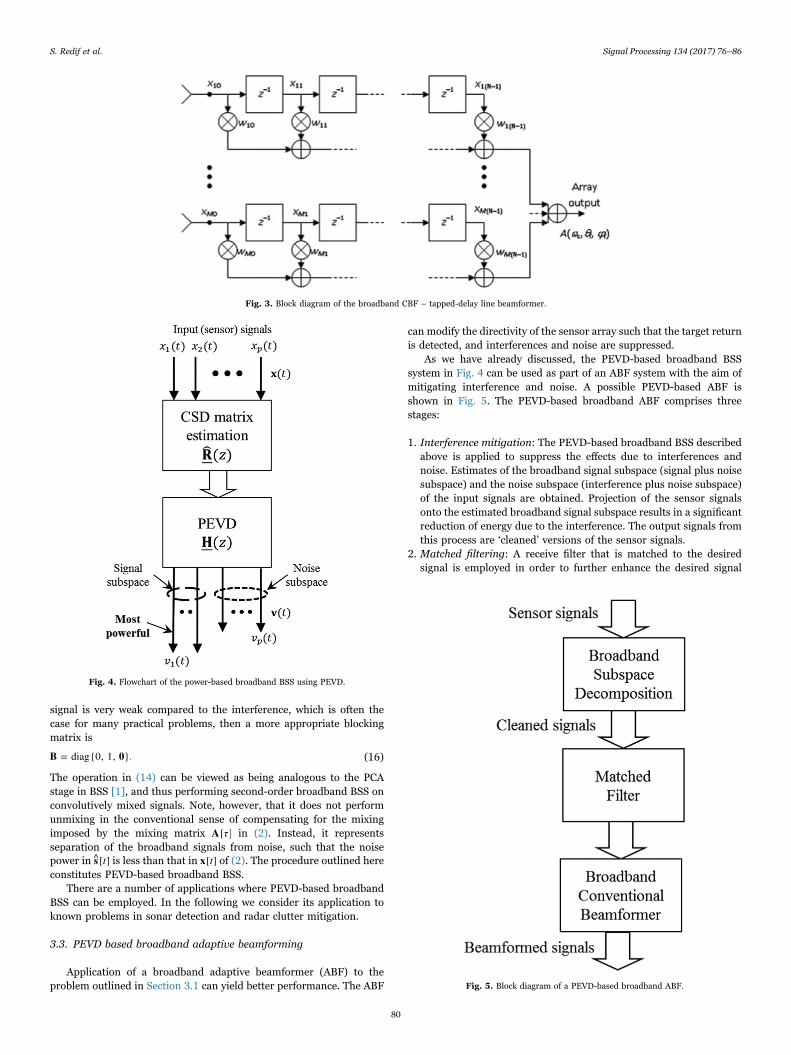
3.4. Example problem I – underwater acoustics

Consider the scenario where a submarine is to be located using a

towed array, as depicted in Fig. 6. The desired signal received by a

passive array is a reflection from the target of the acoustic source signal

transmitted from the towed active array. The reflected signal is a

Doppler-shifted version of the source signal. The passive array also

receives different time-delayed and attenuated versions of the source

signal from different paths due to a reverberant (multipath) environ-

ment. This is usually in the presence of a strong broadband (jamming)

signal produced by the submarine for concealment purposes; this

signal may also be received from different paths. The objective then is

to determine the range and bearing of the target in this severe

environment given measurements from the passive array.

The propagation of the signal sources to the passive array sensors

may be represented in the form of (2). The polynomial mixing matrix

A z( ) describes the convolutive nature of the channel, as well as

encoding the contributions of the source signal to each sensor.

In order to test the PEVD-based broadband ABF described in

Section 3.3, we have performed some computer simulations using real

trials data gathered from a towed array of p=40 hydrophones. The

transmitted signal was a pulsed linear period modulated (LPM) signal

with a pulse length of 0.25 s and a pulse repetition interval (PRI) of

15 s. For each PRI's worth of data a power response (range-bearing

intensity map) of the beamformer was produced. The data is for the

case where a broadband source was used and a continuous-wave (CW)

jamming signal was present. Note that, typically, there were two (man-

made) sources, i.e., q=2: one corresponding to the pulsed LPM and the

other related to the CW tone. However, there were sections of data

where the jammer was switched off, in which case the transmitted LPM

signal was the only artificial source.

In Fig. 7(a), we show responses of the broadband CBF applied with

12 uniformly spaced taps. Each plot is of range versus bearing obtained

by processing the data from a single PRI. From the response of the

broadband CBF we see that it is ineffective at localizing the target,

especially when a broadband jamming signal is present (right). The

jamming signal appears at a single bearing (left hand side plot), but is

spread over a large bandwidth, thus hiding the target return. The

striation is due to leakage through the sidelobes of the broadband CBF

response as the beam is scanned through azimuth.

The performance of the PEVD-based broadband ABF when applied

to the aforementioned sonar problem (Fig. 6) was evaluated by

computer simulation and some results are presented here. In

Fig. 7(b), we show the range-bearing intensity map that results from

processing the data from a single PRI with the PEVD-based algorithm.

Here the PEVD was obtained using the SBR2 algorithm. Also included

in the figure is the response of an IFB approach [56] in Fig. 7(c).

A striking result is that the effects caused by the jamming signal and

reverberation are considerably attenuated with both the PEVD-based

broadband ABF and the IFB approach for the problem considered. For

the case where a jamming signal is present (right hand plots), the

highest intensity points on the range-bearing maps correspond to the

target. For this data set, the PEVD-based broadband ABF method

appears to have suppressed the effects of the jamming signal and the

reverberation slightly more than the IFB approach. Interestingly, in the

case where there is no jamming signal, the target appears clearer for

the plots generated using the PEVD-based broadband ABF compared

to the IFB method. This is because PEVD-based broadband ABF is able

to mitigate the effects due to the reverberation slightly better than the

IFB approach.

It has been shown that the effects due to the reverberation may be

further attenuated by re-application of the PEVD-based broadband BSS

stage in Fig. 4 to the cleaned sensor signals.

3.5. Example problem II – radar clutter suppression

In Fig. 8, an important example of the radar clutter suppression

problem is illustrated. Simulation data was generated for this scenario.

A moving radar device carrying an antenna some distance above a

terrain surface is used to detect an airborne target. The radar antenna

is both a transmitter and a receiver oriented forward towards the

direction of travel. Regular successive pulse transmissions are made

illuminating the area of terrain bounded by the antenna beam.

However, the rough terrain surface within the beam scatters the pulse

energy, a proportion of which is received back at the antenna after a

time delay. The scattered return energy is termed clutter or backscatter.

The aim is to accurately estimate the DoA and Doppler frequency of

the target in the presence of strong and dispersive backscatter from the

ground.

To this end, we applied the PEVD-based broadband ABF described

in Section 3.3 to simulated data, employing SMD to achieve the

factorisation in (10).

The role of the broadband beamformer is to adaptively suppress the

radar clutter with little or no prior knowledge of the target signal or the

clutter. In this light, it may be viewed as performing (second-order)

BSS of broadband (convolutively mixed) signals. An estimate of the

DoA and Doppler frequency of the target is then obtained with the

application of a broadband CBF.

Our simulations were for three different scenarios each with a

target in the presence of clutter and additive white Gaussian noise; the

signal-to-noise ratio (SNR) of the target return in all of the datasets was

0 dB. The target DoA is from an azimuth bearing of +16.7° and an

elevation angle of −3.8°. The datasets correspond to the following three

simulated scenarios:

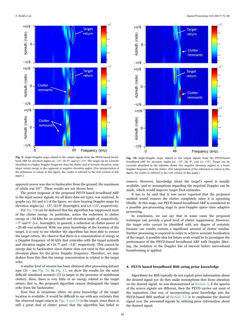
1. The target return is clear of the clutter in terms of Doppler shift at a

higher Doppler frequency (∼60 kHz) than the clutter.

2. The target return is in the sidelobe clutter at a lower Doppler

frequency than the clutter at ∼46 kHz.

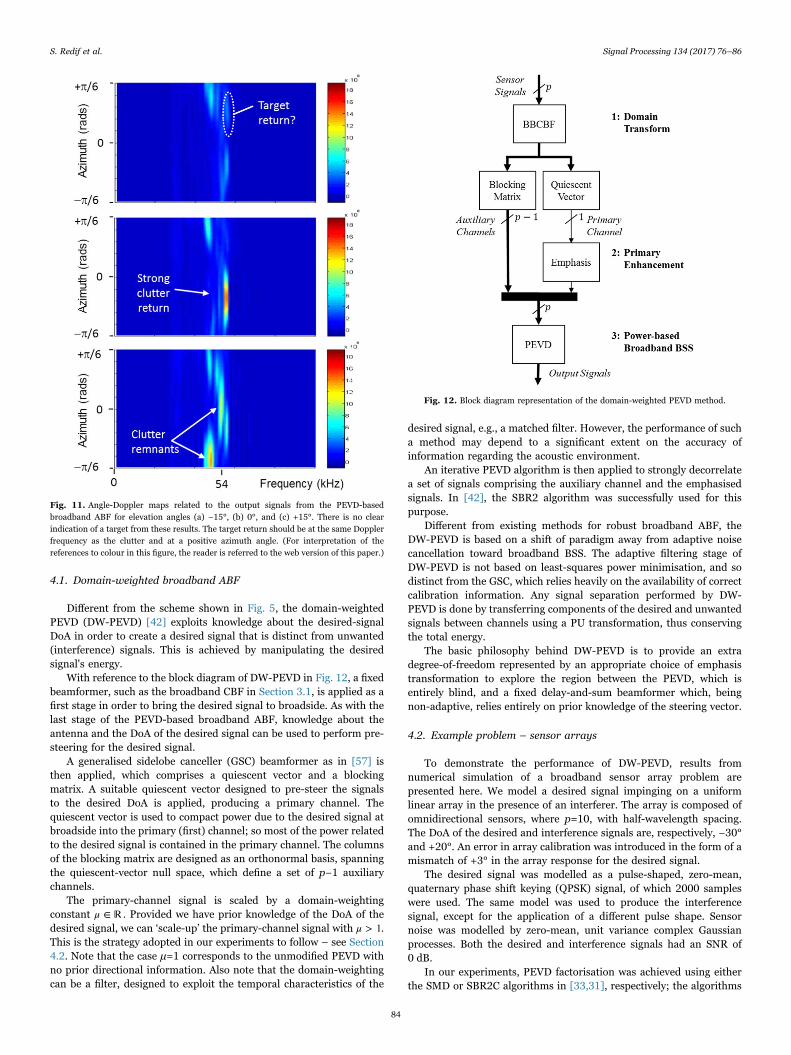
3. The target return is in the mainbeam clutter with the same Doppler

frequency as the clutter, which is ∼54 kHz.

The simulated data is for a moving radar antenna with a 37 element

irregular array operating in a high pulse repetition frequency (PRF)

mode. The PRF=263.8 kHz (2638 pulses) and there are four range

gates. For all datasets, the same clutter signal was used and the SNR of

Fig. 6. Example of sonar detection.

S. Redif et al. Signal Processing 134 (2017) 76–86

81

the clutter was much greater than that of the target return. The target

and clutter models used to produce the synthetic data are realistic,

detail for which is beyond the scope of this paper.

In a practical radar system, the range of the target is tracked over

time, therefore, the range gate that contains the target return is known

a priori. The data from this range gate is collected for processing only.

The attitude and height of the moving radar are unknown and its range

to the target is also unknown.

In Figs. 9–11, graphs of azimuth versus Doppler frequency are

shown, which are referred to as angle-Doppler, or bearing-Doppler,

maps. For each figure, three angle-Doppler maps are shown; each is for

a different elevation angle. The bar to the right of each plot relates the

intensity of the returns to the colours used in the plot; the colour red

signifies a strong return, whereas blue indicates a weak return. The

graphs shown are from images that have been decimated by ten (in the

frequency domain) and concentrated in the Doppler range 0–100 kHz.

As observed for the problem in Section 3.4, analysis of the broad-

band CBF for this problem revealed that, for all three datasets, all of the

Fig. 7. Range-bearing plots for the (a) broadband CBF, (b) PEVD-based broadband ABF and (c) IFB approach applied to data with reverberation present and (left) no jamming signal

and (right) with a strong jamming signal present.

Fig. 8. Example of radar detection.

S. Redif et al. Signal Processing 134 (2017) 76–86

82

apparent power was due to backscatter from the ground, the maximum

of which was 1011. These results are not shown here.

The power response of the proposed PEVD-based broadband ABF

to the input sensor signals, for all three data-set types, was analysed. In

graphs (a), (b) and (c) of the figure, we show bearing-Doppler maps for

elevation angles (a) −15°, (b) 0° (boresight), and (c) +15°, respectively.

For Fig. 9 it can be deduced that the algorithm has suppressed most

of the clutter energy. In particular, notice the reduction in clutter

energy at ∼50 kHz for an azimuth and elevation angle of, respectively,

∼7° and 0o (i.e., boresight); in general, a reduction in clutter power of

∼20 dB was achieved. With our prior knowledge of the location of the

target, it is easy to see whether the algorithm has been able to extract

the target return. We observe that there is a concentration of energy at

a Doppler frequency of 60 kHz that coincides with the target azimuth

and elevation angles of +16.7° and −3.8°, respectively. This cannot be

energy due to backscatter since clutter does not exist in this azimuth-

elevation plane for the given Doppler frequency. Therefore, we may

deduce from this that the energy concentration is related to the target

echo.

A similar level of success has been obtained after processing dataset

type (2) – see Fig. 10. In Fig. 11, we show the results for the most

difficult simulated scenario (3) (a target in the presence of mainbeam

clutter). Here, there is very little or no energy related to the target

return, that is, the proposed algorithm cannot distinguish the target

echo from the backscatter.

Note that in situations where no prior knowledge of the target

location is available, it would be difficult to say with any certainty that

the observed target return in Figs. 9 and 10 is the target, since there is

still a great deal of clutter power that the algorithm has failed to

remove. However, knowledge about the target's speed is usually

available, and so assumptions regarding the required Doppler can be

made, which would improve target DoA estimates.

It has to be said that it was never expected that the proposed

method would remove the clutter completely since it is operating

blindly. At this stage, our PEVD-based broadband ABF is considered as

a possible pre-processing stage to post-Doppler space–time adaptive

processing.

In conclusion, we can say that in some cases the proposed

technique can provide a good level of clutter suppression. However,

the target echo cannot be identified with any degree of certainty

because our results contain a significant amount of clutter residue.

Further processing is required in order to achieve accurate localisation

of the target. A possible idea for future work would be to investigate the

performance of the PEVD-based broadband ABF with Doppler filter-

ing: the isolation of the Doppler bin of interest before narrowband

beamforming is applied.

4. PEVD based broadband BSS using prior knowledge

Algorithms for BSS typically do not exploit prior information about

the desired signal nor do they make assumptions that focus attention

on the desired signal. As was demonstrated in Section 3, if the spectra

of the source signals are different, then the PEVD carries out most of

the separation. One way of incorporating prior knowledge into the

PEVD-based BSS method of Section 3.2 is to emphasise the desired

signal over the unwanted signals by utilizing prior information about

the desired signal.

Fig. 9. Angle-Doppler maps related to the output signals from the PEVD-based broad-

band ABF for elevation angles (a) −15°, (b) 0°, and (c) +15°. The target can be correctly

identified at a higher Doppler frequency than the clutter and at boresite elevation; some

target return energy is also apparent at negative elevation angles. (For interpretation of

the references to colour in this figure, the reader is referred to the web version of this

paper.)

Fig. 10. Angle-Doppler maps related to the output signals from the PEVD-based

broadband ABF for elevation angles (a) −15°, (b) 0°, and (c) +15°. Target can be

correctly identified in the sidelobe clutter (for negative elevation angles) at a lower

Doppler frequency than the clutter. (For interpretation of the references to colour in this

figure, the reader is referred to the web version of this paper.)

S. Redif et al. Signal Processing 134 (2017) 76–86

83

4.1. Domain-weighted broadband ABF

Different from the scheme shown in Fig. 5, the domain-weighted

PEVD (DW-PEVD) [42] exploits knowledge about the desired-signal

DoA in order to create a desired signal that is distinct from unwanted

(interference) signals. This is achieved by manipulating the desired

signal's energy.

With reference to the block diagram of DW-PEVD in Fig. 12, a fixed

beamformer, such as the broadband CBF in Section 3.1, is applied as a

first stage in order to bring the desired signal to broadside. As with the

last stage of the PEVD-based broadband ABF, knowledge about the

antenna and the DoA of the desired signal can be used to perform pre-

steering for the desired signal.

A generalised sidelobe canceller (GSC) beamformer as in [57] is

then applied, which comprises a quiescent vector and a blocking

matrix. A suitable quiescent vector designed to pre-steer the signals

to the desired DoA is applied, producing a primary channel. The

quiescent vector is used to compact power due to the desired signal at

broadside into the primary (first) channel; so most of the power related

to the desired signal is contained in the primary channel. The columns

of the blocking matrix are designed as an orthonormal basis, spanning

the quiescent-vector null space, which define a set of p−1 auxiliary

channels.

The primary-channel signal is scaled by a domain-weighting

constant μ ∈ . Provided we have prior knowledge of the DoA of the

desired signal, we can ‘scale-up’ the primary-channel signal with μ > 1.This is the strategy adopted in our experiments to follow – see Section

4.2. Note that the case μ=1 corresponds to the unmodified PEVD with

no prior directional information. Also note that the domain-weighting

can be a filter, designed to exploit the temporal characteristics of the

desired signal, e.g., a matched filter. However, the performance of such

a method may depend to a significant extent on the accuracy of

information regarding the acoustic environment.

An iterative PEVD algorithm is then applied to strongly decorrelate

a set of signals comprising the auxiliary channel and the emphasised

signals. In [42], the SBR2 algorithm was successfully used for this

purpose.

Different from existing methods for robust broadband ABF, the

DW-PEVD is based on a shift of paradigm away from adaptive noise

cancellation toward broadband BSS. The adaptive filtering stage of

DW-PEVD is not based on least-squares power minimisation, and so

distinct from the GSC, which relies heavily on the availability of correct

calibration information. Any signal separation performed by DW-

PEVD is done by transferring components of the desired and unwanted

signals between channels using a PU transformation, thus conserving

the total energy.

The basic philosophy behind DW-PEVD is to provide an extra

degree-of-freedom represented by an appropriate choice of emphasis

transformation to explore the region between the PEVD, which is

entirely blind, and a fixed delay-and-sum beamformer which, being

non-adaptive, relies entirely on prior knowledge of the steering vector.

4.2. Example problem – sensor arrays

To demonstrate the performance of DW-PEVD, results from

numerical simulation of a broadband sensor array problem are

presented here. We model a desired signal impinging on a uniform

linear array in the presence of an interferer. The array is composed of

omnidirectional sensors, where p=10, with half-wavelength spacing.

The DoA of the desired and interference signals are, respectively, −30°

and +20°. An error in array calibration was introduced in the form of a

mismatch of +3° in the array response for the desired signal.

The desired signal was modelled as a pulse-shaped, zero-mean,

quaternary phase shift keying (QPSK) signal, of which 2000 samples

were used. The same model was used to produce the interference

signal, except for the application of a different pulse shape. Sensor

noise was modelled by zero-mean, unit variance complex Gaussian

processes. Both the desired and interference signals had an SNR of

0 dB.

In our experiments, PEVD factorisation was achieved using either

the SMD or SBR2C algorithms in [33,31], respectively; the algorithms

Fig. 11. Angle-Doppler maps related to the output signals from the PEVD-based

broadband ABF for elevation angles (a) −15°, (b) 0°, and (c) +15°. There is no clear

indication of a target from these results. The target return should be at the same Doppler

frequency as the clutter and at a positive azimuth angle. (For interpretation of the

references to colour in this figure, the reader is referred to the web version of this paper.)

Fig. 12. Block diagram representation of the domain-weighted PEVD method.

S. Redif et al. Signal Processing 134 (2017) 76–86

84

were allowed to run for 50 iterations. A scalar domain-weighting was

applied as the primary enhancement, using only μ=1 or μ=2.

The power response of the overall system in Fig. 12 — convolution

of all transformations from sensors to the PEVD — is shown, for three

experiments, in Figs. 13–15. Each plot in a figure shows the power of

the beam (beampatterns), for different azimuthal angles of arrival and

frequency. The top two plots of each figure are the beampatterns for the

first and second rows of the transform matrix, respectively, for the

whole DW-PEVD system. The third plot is an average beampattern

over the rows 3 to p of the matrix. The bar to the right of each plot

indicates power level in dBs; white signifies the highest power level,

whereas black indicates the lowest power.

Fig. 13 is for the case where no primary enhancement was used, i.e.,

μ=1. It is clear that the unweighted DW-PEVD cannot perform a good

level of signal separation since there is considerable leakage of the look-

direction signal into the second channel and the interference signal into

the first channel. This is consistent with the theory presented earlier in

this section.

In Fig. 14, we show beampatterns for the beamformer with a

primary enhancement setting of μ=2 for the same scenario. We can see

that the DW-PEVD has designed a first beam which points to the

desired signal; the second beam, which is orthogonal to the first, is

designed to point in the direction of the interferer. The other beams are

orthogonal to the first two beams, as is indicated by very low

intensities.

We see that varying the value of μ provides an additional degree-of-

freedom for achieving good signal separation, and hence interference

suppression. Simulation results from assessing the influence of μ have

revealed that the DW-PEVD performance has very little dependence on

μ at large SNRs. These results are not provided here – the reader is

referred to [41] for a thorough characterisation.

In Fig. 15, beampatterns for a beamformer based on the subband-

coding variant of SBR2, or the SBR2C algorithm, with a setting of μ=1,

for the same scenario, is shown. Notice that even though there is no

emphasis on the primary channel, the algorithm does fairly well in

separating the two signals, whilst also correctly identifying each signal's

DoA.

The improved performance is due to the fact that SBR2C is

proportionately equally sensitive to changes in any of the signals

[31,41]. While systems with a priori knowledge will usually perform

better, the SBR2C-based system is able to recover the signals and their

DoAs without this knowledge.

5. Conclusions

The overarching goal of this paper has been to build intuition and

insight into the important field of polynomial matrix decompositions

and its relevance to broadband BSS while leaving the detail to

references.

Sample applications in the areas of broadband BSS and beamform-

ing have been presented along with solutions and new results to three

important problems via a polynomial EVD based broadband beamfor-

mer and a domain-weighted polynomial EVD. The results have been

compared to those of classical broadband methods, which highlights

the suitability of the polynomial EVD to the problem of broadband BSS.

Acknowledgements

This work was supported in parts by the Engineering and Physical

Sciences Research Council (EPSRC) Grant number EP/K014307/1 and

the MOD University Defence Research Collaboration in Signal

Processing.

References

[1] P. Comon, Independent component analysis, a new concept?, Signal Process. 36

(April (3)) (1994) 287–314.

[2] A. Hyvarinen, J. Karhunen, E. Oja, Independent Component Analysis, John Wiley

and Sons, NY, 2001.

[3] G.H. Golub, C.F. Van Loan, Matrix Computations, 3rd edition, John Hopkins

University Press, Baltimore, Maryland, 1996.

[4] S. Haykin, Adaptive Filter Theory, 4th edition, Prentice Hall, Englewood Cliffs, NJ,

2002.

Fig. 13. Beampatterns of the DW-PEVD using SMD, for the case when

SNR = INR = 0 dB and for μ=1.

Fig. 14. Beampatterns of the DW-PEVD using SMD, for the case when

SNR = INR = 0 dB and for μ=2.

Fig. 15. Beampatterns of the DW-PEVD using SBR2C, for the case when

SNR = INR = 0 dB and μ=1.

S. Redif et al. Signal Processing 134 (2017) 76–86

85

[5] J. Bobin, J.-L. Starck, M.J. Fadili, Y. Moudden, Sparsity and morphological

diversity in blind source separation, IEEE Trans. Image Process. 16 (November

(11)) (2007) 2662–2674.

[6] J. Zhang, H. Zhang, L. Wei, Y.J. Wang, Blind source separation with pattern

expression NMF, in: Advances in Neural Networks ISNN 2006, Springer-Verlag,

Heidelberg, 2006, vol. 3971, pp. 1159–1164.

[7] A.S. Montcuquet, L. Hervé, F. Navarro, J.M. Dinten, J.I. Mars, Nonnegative matrix

factorization: a blind spectra separation method for in vivo fluorescent optical

imaging, J. Biomed. Opt. 15 (September (5)) (2010) 056009.

[8] B.M. Abadi, A. Sarrafzadeh, F. Ghaderi, S. Sanei, Semi-blind channel estimation in

MIMO communication by tensor factorization, in: IEEE Workshop on Statistical

Signal Processing, August 2009, pp. 313–316.

[9] P.P. Vaidyanathan, Theory of optimal orthonormal subband coders, IEEE Trans.

Signal Process. 46 (June (6)) (1998) 1528–1543.

[10] P. Smaragdis, Blind separation of convolved mixtures in the frequency domain,

Neurocomputing 22 (1998) 21–34.

[11] S. Ikeda, N. Murata, A method of ICA in time–frequency domain, in: Workshop on

Independent Component Analysis and Signal Separation, 1999, pp. 365–370.

[12] H. Wang, M. Kaveh, Coherent signal-subspace processing for the detection and

estimation of angles of arrival of multiple wide-band sources, IEEE Trans. Acoust.

Speech Signal Process. 33 (August (4)) (1985) 823–831.

[13] H. Hung, M. Kaveh, Focussing matrices for coherent signal-subspace processing,

IEEE Trans. Acoust. Speech Signal Process. 36 (August (8)) (1988) 1272–1281.

[14] Y. Bucris, I. Cohen, M.A. Doron, Bayesian focusing for coherent wideband

beamforming, IEEE Trans. Audio Speech Lang. Process. 20 (May (4)) (2012)

1282–1296.

[15] T. Kailath, Linear Systems, Prentice Hall, Englewood Cliffs, NJ, 1980.

[16] R.H. Lambert, M. Joho, H. Mathis, Polynomial singular values for number of

wideband source estimation and principal components analysis, in: Proceedings of

International Conference on Independent Component Analysis, 2001, pp. 379–

383.

[17] R.H. Lambert, Multichannel blind deconvolution: FIR matrix algebra and separa-

tion of multipath mixtures (Ph.D. thesis), University Southern California, LA, 1996.

[18] P.A. Regalia, P. Loubaton, Rational subspace estimation using adaptive lossless

filters, IEEE Trans. Signal Process. 40 (October (10)) (1992) 2392–2405.

[19] P.P. Vaidyanathan, Multirate Systems and Filter Banks, Prentice Hall, Englewood

Cliffs, 1993.

[20] P. Desarte, B. Macq, D.T.M. Slock, Signal-adapted multiresolution transform for

image coding, IEEE Trans. Inf. Theory 38 (March (2)) (1992) 897–904.

[21] P.A. Regalia, D.-Y. Huang, Attainable error bounds in multirate adaptive lossless

FIR filters, in: Proceedings of IEEE Conference on Acoustics, Speech, and Signal

Processing, 1995, pp. 1460–1463.

[22] P. Moulin, M.K. Mihcak, Theory and design of signal-adapted FIR paraunitary filter

banks, IEEE Trans. Signal Process. 46 (April (4)) (1998) 920–929.

[23] B. Xuan, R.I. Bamberger, FIR principal component filter banks, IEEE Trans. Signal

Process. 46 (April (4)) (1998) 930–940.

[24] X. Gao, T.Q. Nguyen, G. Strang, On factorization of M-channel paraunitary

filterbanks, IEEE Trans. Signal Process. 49 (July (7)) (2001) 1433–1446.

[25] J.G. McWhirter, P.D. Baxter, A novel technique for broadband SVD, in: 12th

Annual Workshop Adaptive Sensor Array Processing, MIT Lincoln Labs,

Cambridge, MA, 2004.

[26] J.G. McWhirter, P.D. Baxter, T. Cooper, S. Redif, J. Foster, An EVD algorithm for

para-Hermitian polynomial matrices, IEEE Trans. Signal Process. 55 (May (5))

(2007) 2158–2169.

[27] A. Tkacenko, P.P. Vaidyanathan, Iterative greedy algorithm for solving the FIR

paraunitary approximation problem, IEEE Trans. Signal Process. 54 (January (1))

(2006) 146–160.

[28] A. Tkacenko, Approximate eigenvalue decomposition of para-Hermitian systems

through successive FIR paraunitary transformations, in: IEEE International

Conference on Acoustics Speech, and Signal Processing, March 2010, pp. 4074–

4077.

[29] J.G. McWhirter, An algorithm for polynomial matrix SVD based on generalised

Kogbetliantz transformations, in: European Signal Processing Conference, Aalborg,

Denmark, 2010, pp. 457–461.

[30] J.A. Foster, J.G. McWhirter, M.R. Davies, J.A. Chambers, An algorithm for

calculating the QR and singular value decompositions of polynomial matrices, IEEE

Trans. Signal Process. 58 (March (3)) (2010) 1263–1274.

[31] S. Redif, J.G. McWhirter, S. Weiss, Design of FIR paraunitary filter banks for

subband coding using a polynomial eigenvalue decomposition, IEEE Trans. Signal

Process. 59 (November (11)) (2011) 5253–5264.

[32] S. Redif, S. Weiss, J.G. McWhirter, An approximate polynomial matrix eigenvalue

decomposition algorithm for para-Hermitian matrices, in: IEEE 11th International

Symposium on Signal Processing and Information Technology, Bilbao, Spain, 2011,

pp. 421–425.

[33] S. Redif, S. Weiss, J.G. McWhirter, Sequential matrix diagonalisation algorithms

for polynomial EVD of parahermitian matrices, IEEE Trans. Signal Process. 63

(January (1)) (2015) 81–89.

[34] S. Icart, P. Comon, Some properties of Laurent polynomial matrices, in: 9th IMA

Conference on Mathematics in Signal Processing, Birmingham, UK, December

2012.

[35] S. Kasap, S. Redif, Novel field-programmable gate array architecture for computing

the eigenvalue decomposition of para-Hermitian polynomial matrices, IEEE Trans.

Very Large Scale Integr. Syst. 22 (March (3)) (2014) 522–536.

[36] J. Corr, K. Thomson, S. Weiss, J.G. McWhirter, S. Redif, I.K. Proudler, Multiple

shift maximum element sequential matrix diagonalisation for parahermitian

matrices, in: IEEE Workshop on Statistical Signal Processing, Gold Coast,

Australia, July 2014, pp. 312–315.

[37] Z. Wang, J.G. McWhirter, J. Corr, S. Weiss, Multiple shift second order sequential

best rotation algorithm for polynomial matrix eigenvalue decomposition, in: IEEE

European Signal Processing Conference, Nice, France, August 2015, pp. 844–848.

[38] M. Tohidian, H. Amindavar, A.M. Reza, A DFT-based approximate eigenvalue and

singular value decomposition of polynomial matrices, EURASIP J. Adv. Signal

Process. 1 (2013) 1–16.

[39] R. Brandt, M. Bengtsson, Wideband MIMO channel diagonalization in the time

domain, in: International Symposium on Personal, Indoor and Mobile Radio

Communications, 2011, pp. 1914–1918.

[40] J. Corr, K. Thompson, S. Weiss, I.K. Proudler, J.G. McWhirter, Shortening of

paraunitary matrices obtained by polynomial eigenvalue decomposition algorithms,

in: 5th Conference of the Sensor Signal Processing for Defence, Edinburgh, UK,

July 2015.

[41] S. Redif, Polynomial matrix decomposition and paraunitary filter banks (Ph.D.

thesis), University of Southampton, 2006.

[42] S. Redif, J.G. McWhirter, P.D. Baxter, T. Cooper, Robust broadband adaptive

beamforming via polynomial eigenvalues, in: IEEE/MTS OCEANS'06, Boston, MA,

September 2006, pp. 1–6.

[43] S. Redif, U. Fahrioglu, Foetal ECG extraction using broadband signal subspace

decomposition, in: IEEE Mediterranean Microwave Symposium, Guzelyurt,

Cyprus, 2010. pp. 381–84.

[44] M.A. Alrmah, S. Weiss, S. Lambotharan, An extension of the MUSIC algorithm to

broadband scenarios using polynomial eigenvalue decomposition, in: 19th

European Signal Processing Conference, Spain, September 2011, pp. 629–633.

[45] M. Alrmah, S. Weiss, S. Redif, S. Lambotharan, J.G. McWhirter, M. Kaveh, Angle of

arrival estimation for broadband signals: a comparison, in: IET Intelligent Signal

Processing Conference, London, UK, December 2013.

[46] S. Redif, Fetal electrocardiogram estimation using polynomial eigenvalue decom-

position, Turk. J. Electr. Eng. Comput. Sci. 24 (August (4)) (2014) 2483–2497.

[47] S. Weiss, S. Bendoukha, A. Alzin, F. Coutts, I. Proudler, J. Chambers, MVDR

broadband beamforming using polynomial matrix techniques, in: 23rd European

Signal Processing Conference, Nice, France, September 2015, pp. 844–848.

[48] S. Weiss, S. Redif, T. Cooper, C. Liu, P. Baxter, J.G. McWhirter, Paraunitary

oversampled filter bank design for channel coding, EURASIP J. Appl. Signal

Process 2006 (2006) 1–10. http://dx.doi.org/10.1155/ASP/2006/31346 ID 31346.

[49] J. Foster, J. McWhirter, S. Lambotharan, I. Proudler, M. Davies, J. Chambers,

Polynomial matrix QR decomposition for the decoding of frequency selective

multiple-input multiple-output communication channels, IET Signal Process. 6

(September (7)) (2012) 704–712.

[50] Z. Wang, J.G. McWhirter, S. Weiss, Multichannel spectral factorization algorithm

using polynomial matrix eigenvalue decomposition, in: Asilomar Conference on

Signals, Systems, and Computers, 2015.

[51] S. Redif, S. Kasap, Novel reconfigurable hardware architecture for polynomial

matrix multiplications, IEEE Trans. Very Large Scale Integr. Syst. 23 (March (3))

(2015) 454–465.

[52] P.D. Baxter, J.G. McWhirter, Robust adaptive beamforming based on domain

weighted PCA, in: 13th European Signal Processing Conference, Antalya, Turkey,

2005.

[53] G.D. Clifford, Singularvalue decomposition and independent component analysis

for blind signal separation, Bio Signal Image Process. 44 (6) (2005) 489–499.

[54] H.L. Van Trees, Detection, Estimation and Modulation Theory, Wiley & Sons Inc.,

USA, 1968 ISBNs: 0-471-09517-6.

[55] J.-P. Hermand, W.I. Roderick, Acoustic model-based matched filter processing for

fading time-dispersive ocean channels: theory and experiment, IEEE Trans. Ocean.

Eng. 18 (October (4)) (1993) 447–465.

[56] R. Klemm, Space–Time Adaptive Processing Principles and Applications, Series 9,

IEE Radar, Sonar, Navigation and Avionics, London, UK, 1998.

[57] L.J. Griffiths, C.W. Jim, An alternative approach to linearly constrained adaptive

beamforming, IEEE Trans. Antennas Propag. 30 (January (1)) (1982) 27–34.

S. Redif et al. Signal Processing 134 (2017) 76–86

86