redalyc.analysis of large distribution networks with distributed

Ingeniare. Revista Chilena de Ingeniería

ISSN: 0718-3291

[email protected]

Universidad de Tarapacá

Chile

Martínez-Velasco, Juan A.; Guerra, Gerardo

Analysis of large distribution networks with distributed energy resources

Ingeniare. Revista Chilena de Ingeniería, vol. 23, núm. 4, octubre, 2015, pp. 594-608

Universidad de Tarapacá

Arica, Chile

Available in: http://www.redalyc.org/articulo.oa?id=77242864010

How to cite

Complete issue

More information about this article

Journal's homepage in redalyc.org

Scientific Information System

Network of Scientific Journals from Latin America, the Caribbean, Spain and Portugal

Non-profit academic project, developed under the open access initiative

http://www.redalyc.org/revista.oa?id=772


http://www.redalyc.org/articulo.oa?id=77242864010

http://www.redalyc.org/comocitar.oa?id=77242864010

http://www.redalyc.org/fasciculo.oa?id=772&numero=42864

http://www.redalyc.org/articulo.oa?id=77242864010


http://www.redalyc.org

Ingeniare. Revista chilena de ingeniería, vol. 23 Nº 4, 2015, pp. 594-608

Analysis of large distribution networks with distributed energy resources

Análisis de grandes redes de distribución con recursos energéticos distribuidos

Juan A. Martínez-Velasco1 Gerardo Guerra1

Recibido 27 de junio de 2014, aceptado 22 de diciembre de 2014Received: June 27, 2014 Accepted: December 22, 2014

ABSTRACT

The connection of distributed energy resources (i.e., distributed generation and energy storage) and some special loads (e.g., electrical vehicle) raises new challenges in distribution system analysis. Intermittent and non-dispatchable generation units, time-dependent or asymmetrical loads require capabilities that until very recently were not available in distribution software packages; for instance, capabilities for probabilistic and time mode simulations. This paper presents the work made by the authors to adapt OpenDSS, a freely available distribution simulator, in order to perform these types of studies taking into account that the model of an actual distribution system is usually very large and complex. A goal of the paper is to present the usage of OpenDSS as either a stand-alone tool or as a COM DLL driven from MATLAB. Several applications have been developed to obtain yearly curve shapes aimed at representing time-varying loads and renewable energy sources (sun, wind) and to run OpenDSS in a distributed computing environment (e.g., multicore installation).

Keywords: Distribution network, distributed energy resources, probabilistic analysis, parallel computing.

RESUMEN

La conexión de recursos energéticos distribuidos (es decir, generación distribuida y almacenamiento de energía) y algunas demandas especiales (por ejemplo, el coche eléctrico) generan nuevos retos en el análisis y simulación de redes de distribución. Unidades con generación intermitente, así como demandas variables en el tiempo o asimétricas, requieren nuevas prestaciones que hasta muy recientemente no han estado disponibles en herramientas de simulación de redes de distribución; por ejemplo, prestaciones para llevar a cabo simulaciones probabilísticas o en función del tiempo. Este artículo presenta el trabajo realizado por los autores para adaptar OpenDSS, un simulador libre de análisis de redes de distribución, y poder realizar este tipo de estudios teniendo en cuenta que el modelo de la red de distribución es en general muy grande y complejo. El objetivo principal de este trabajo es presentar la aplicación de OpenDSS, funcionando como herramienta autónoma o controlada desde MATLAB, en el análisis y diseño de grandes redes de distribución. Varias aplicaciones han sido desarrolladas para obtener las curvas anuales de demanda y generación renovable (solar, eólica) y poder ejecutar OpenDSS en un entorno de cálculo distribuido; es decir, en una instalación con múltiples procesadores funcionando en paralelo.

Palabras clave: Red de distribución, recursos energéticos distribuidos, análisis probabilístico, cálculo paralelo.

1 Departament d’Enginyeria Elèctrica. Universitat Politècnica de Catalunya. Av. Diagonal 647, CP 08028. Barcelona, España. E-mail: [email protected]; [email protected]

Martínez-Velasco and Guerra: Analysis of large distribution networks with distributed energy resources

595

INTRODUCTION

Distribution system analysis has been traditionally perceived as the study of rather small radially-connected systems by means of dedicated simple power flow methods. This perception has dramatically changed during the last decade. Actual distribution systems are very complex, even more complex than transmission systems, and several software packages are presently available for realistic analysis of distribution systems. The list of essential capabilities implemented in current simulation packages for distribution system analysis may include the following items [1-3]:

· mixture of three-phase, two-phase and single-phase distribution system component models;

· capabilities to perform simulations of radial and meshed networks over periods of time (e.g., one year);

· built-in ZIP models of end use loads;· representation of distributed generation and

energy storage devices.

Basic issues addressed in most distribution system simulators include power flow solution methods, steady-state short circuit calculations, and reliability analysis. In general, dynamics analysis is not commonly implemented in tools for distribution system analysis, although some include harmonic analysis. In addition, modelling approaches generally ignore the secondary (LV) distribution system. Although present tools and techniques are designed for uniprocessors (e.g., single CPU) they can easily cope with rather large distribution systems (e.g., several thousands of nodes).

It is foreseen that the future (smart) distribution system will monitor, protect, and automatically optimize the operation of its interconnected elements to maintain a reliable and secure infrastructure that can meet future demand growth [4-6]. Such a grid will offer improved reliability, higher asset utilization, better integration of distributed energy resources (DERs) and new loads (e.g., plug-in hybrid electric vehicles), reduced operating costs, increased efficiency and conservation, and lower greenhouse gas emissions.

An important aspect of the future grid would be the high penetration of DERs which can be used

for supporting voltage, reducing losses, providing backup power, improving local power quality and reliability, providing ancillary services, and deferring distribution system upgrade [7-9]. Aspects to be considered when analysing the connection of DERs are the great variety of generating and energy storage devices [8, 10], the fact that some DER devices are connected to the utility network via a static converter [11], and the intermittent nature of some renewable sources.

DERs raise several challenges to distribution load flow calculations since they demand modelling capabilities for representing intermit-tent generators, energy storage devices, voltage-control equipment, or multi-phase unbalanced systems. In addition, studies of systems with non-dispatchable resources will require a probabilistic approach and calculations performed over an arbitrary time period that may range from several minutes to several years.

Load representation is another important issue since voltage-dependent loads with random variation and a duration curve must be also accounted for. These issues complicate the study since software tools have to combine new analysis capabilities with a high number of models for representing the various generation and energy storage technologies, besides the conventional distribution system components, and include capabilities for time mode calculations [10].

The essential requirements for future distribution system analysis software may be summarized as follows [12-13]: (1) perform fast solutions, (2) be able to capture and process voluminous amounts of simulation results, (3) have robust solution methods for simulating both radial and meshed networks, (4) be able to perform time series simulations with time steps as short as 1 second during periods of several years, (5) solve very large distribution networks, (6) be able to include higher voltage sub-transmission and transmission systems, (7) provide data on end-use patterns for better quantification of distribution system efficiency and improving automation simulations. The list of foreseen functionalities will include grid reconfiguration, state estimation, look-ahead analysis and visualization, contingencies analysis, and load forecasting.

This paper is aimed at presenting the work carried out by the authors to implement some of

Ingeniare. Revista chilena de ingeniería, vol. 23 Nº 4, 2015

596

the functionalities required for analysing large distribution systems with distributed generation. The simulation tool used for this purpose is OpenDSS, a freely available distribution system simulator, whose modelling and calculation capabilities allow users to represent the most important distribution components and perform studies considering both deterministic and probabilistic calculations [14].

The paper presents: (i) the application of OpenDSS to the study of distribution systems with renewable generation and time-varying loads, (ii) an introduction to the algorithms implemented in MATLAB by the authors for obtaining yearly curve shapes of loads and renewable generation (sun, wind), and (iii) the application of a MATLAB-OpenDSS link for optimum allocation of renewable generation in large distribution systems using a Parallel Monte Carlo approach.

APPLICATION OF OPENDSS

IntroductionOpenDSS is a simulation tool for analysis of electric utility distribution systems, implemented as both a stand-alone executable program and a COM DLL that can be driven from some software platforms. The executable version adds a basic user interface onto the solution engine to assist users in developing scripts and viewing solutions [14]. Built-in solution capabilities include snapshot and time mode power flow, harmonics, fault current study, dynamics, parametric and probabilistic studies.

OpenDSS can be used for distribution planning and analysis, using a general multi-phase AC circuit model, including models for renewable energy resources, energy storage devices, or unusual transformer configurations. Other solution techniques and capabilities (e.g., graphics) can be added through the COM interface [14-16]. This paper presents how this interface can be used to drive OpenDSS from MATLAB.

External tools can be used to generate load and intermittent generation (wind, solar) curve shapes, mainly when the period to be analyzed is too long (e.g., one year). Supporting tools can be also required when a probabilistic approach is to be used for generating random values of loads and generations according to a specific probability density

function (e.g., Weibull). In the study presented in this section, these curves have been obtained by means of HOMER (Hybrid Optimization Model for Electric Renewables) [17-18]. This tool can synthesize load, wind and solar data over a period of one year using a variable time step. Time-varying curves generated with HOMER can be easily adapted for representing power demand and generation in an OpenDSS input file.

OpenDSS plotting capabilities can be used also for displaying input loadshapes and generation curves. On the other hand, random values can be generated from within the simulator, without using any external support. The tool generates a great variety of output files, which can be easily manipulated to display simulation results (e.g., voltages, currents, powers, overloads, over- and undervoltages, or energy losses).

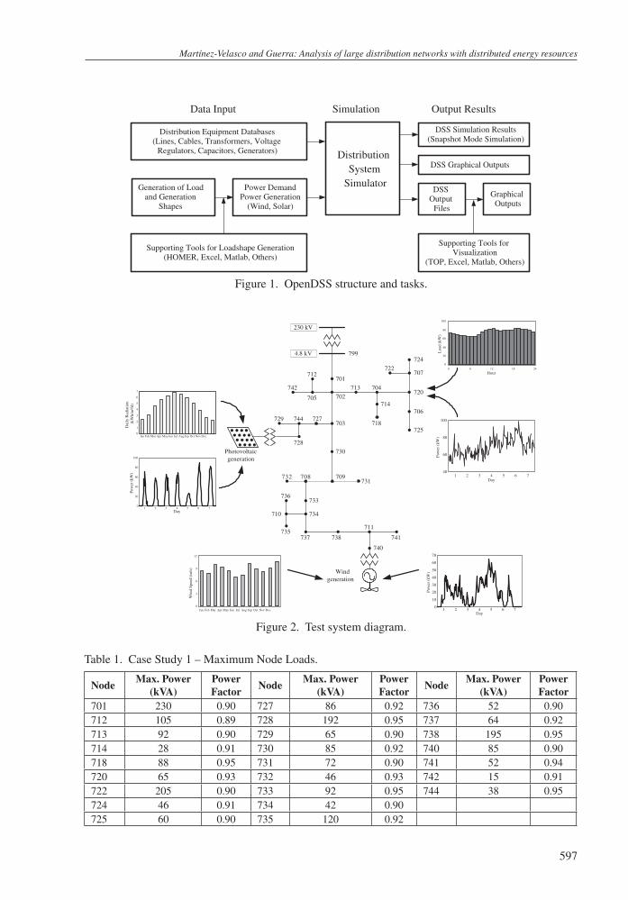
Case studies and simulation resultsFigure 1 shows the organization of tasks between tools, as used for this study. Figure 2 shows the diagram of the test distribution system [19]. It is based on the IEEE37 test feeder, which consists of three-phase underground cables operating at a nominal voltage of 4.8 kV. Characteristics of cable sections were presented in [20]. Notice that some renewable energy generation units are connected to this feeder.

Two different scenarios have been analyzed [19]: (i) test system with time-varying load; (ii) test system with probabilistic load. The two studies assume balanced loads. In both cases, calculations are made with and without generation.

Case Study 1 - Distributed Generation Impact: Table 1 shows the maximum node load demands. As mentioned above, to represent time-varying loads different yearly curve shapes were created using HOMER. Each of these shapes was then assigned to some feeder nodes. The calculations were performed by assuming that the power factor at each node load remains constant during the simulation period.

Figure 3 shows the daily profile and the resulting power of one load shape during one month. Two renewable generators were connected to the system, as shown in Figure 2. A 400 kW wind power generator is connected to Node 740 and a 200 kW


597

Distribution Equipment Databases(Lines, Cables, Transformers, Voltage

Regulators, Capacitors, Generators)

Power DemandPower Generation

(Wind, Solar)

Generation of Load and Generation

Shapes

Data Input Simulation

Distribution System

Simulator

DSS Graphical Outputs

DSS Output

Files

Graphical Outputs

Output Results

Supporting Tools for Visualization

(TOP, Excel, Matlab, Others)

Supporting Tools for Loadshape Generation(HOMER, Excel, Matlab, Others)

DSS Simulation Results(Snapshot Mode Simulation)

Figure 1. OpenDSS structure and tasks.

799

701

742

705 702720

704713

707722

703744729

728

727706

725718

714

730

731709237 807

733736

734710

735737 738

711

741

740

724

712

Windgeneration

Photovoltaicgeneration

230 kV

4.8 kV

Jan Feb Mar Apr May Jun Jul AugSep Oct Nov Dec0

1

2

3

4

5

6

7

Dai

ly R

adia

tion

(kW

h/m

2/d)

Day1 2 3 4 5 6 7

0

20

40

60

80

100

Pow

er (

kW)

1 2 3 4 5 6 70

10

20

30

40

50

60

70

Pow

er (

kW)

DayJan Feb Mar Apr May Jun Jul Aug Sep Oct Nov Dec

0

3

6

9

12

Win

d S

peed

(m

/s)

0 6 12 18 24

0

20

40

60

80

100

Loa

d (k

W)

Hour

Day1 2 3 4 5 6 7

40

60

80

100

Pow

er (

kW)

Figure 2. Test system diagram.

Table 1. Case Study 1 – Maximum Node Loads.

NodeMax. Power

(kVA)Power Factor

NodeMax. Power

(kVA)Power Factor

NodeMax. Power

(kVA)Power Factor

701 230 0.90 727 86 0.92 736 52 0.90712 105 0.89 728 192 0.95 737 64 0.92713 92 0.90 729 65 0.90 738 195 0.95714 28 0.91 730 85 0.92 740 85 0.90718 88 0.95 731 72 0.90 741 52 0.94720 65 0.93 732 46 0.93 742 15 0.91722 205 0.90 733 92 0.95 744 38 0.95724 46 0.91 734 42 0.90725 60 0.90 735 120 0.92


598

photovoltaic generator is connected to Node 728. In both cases, the power factor of the injected power is unity. Figures 4 and 5 show the wind and solar resources at the distribution system location. As for the load shapes, HOMER capabilities were initially used to obtain the wind speed (see Figure 4) and the solar radiation (see Figure 5). These profiles were later used to derive the shapes of the power injected by both generators, see Figure 6.

The main goal of this first study is to compare results when using different approaches to represent loads, which (1) are assumed to be voltage independent, or (2) represented as constant impedances. Figure 7 shows some simulation results without generation. According to this figure, differences are not very important for the kVAs measured at Node 728.

However, the differences may be up to 10% for the power flow measured at the feeder head. According to Figure 8a, the values of the energy supplied during the entire year and without DG are respectively 8300 and 7723 MWh with the constant PQ model and the quadratic PQ (i.e., the results differ in about 7%); the minimum voltages with the two models are respectively 0.915 and 0.924 pu. Figure 8b shows that the differences with DG are again about 10%. As for the energy supplied from the substation, the values corresponding to each load model are now 7336 and 6792 MWh. That is, embedded generators take a 10% of the required energy, and the differences between models are again of about 7%. The connection of generators raises the minimum voltages to 0.922 and 0.930 pu.

Case Study 2 - Probabilistic Load Flow Calculations: Load and generation values are generally estimated

0 6 12 18 240.0

0.2

0.4

0.6

0.8

1.0Daily Pro�le

Hour

Monthly load

Figure 3. Case Study 1. Load profiles.

Jan Feb Mar Apr May Jun Jul Aug Sep Oct Nov Dec0

3

6

9

12

Win

d Sp

eed

(m/s

)

Figure 4. Case Study 1. Wind resource-Wind speed (m/s).

Jan Feb Mar Apr May Jun Jul Aug Sep Oct Nov Dec0

1

2

3

4

5

6

7

Dai

ly R

adia

tion

(kW

h/m

2/d)

Figure 5. Case Study 1. Solar resource-Daily radiation (kWh/m2/d).

0

30

60

90

120

150

1800 1820 1840 1860 1880 1900

Pow

er (

kW)

Wind

Photovoltaic

Figure 6. Case Study 1. Distributed generation-Phase A.

60

50

40

30

20

500 520 540Hour

Pow

er (k

VA

)

Quadratic P-Q

Constant P-Q

560 580 600

10

0

Figure 7. Case Study 1. Load at Node 728 (kVA).


599

or calculated with some uncertainties, in which case a probabilistic calculation may be considered. A load flow based on the Monte Carlo method is an option implemented in OpenDSS.

Table 2 shows the probability density functions assumed for loads and generations, as well as the parameters selected for each load and each generator. Notice that a Weibull distribution is generally assumed for the wind speed [21]. This distribution is further used to derive the power generation from the power curve of the wind turbine, taking into account air density ratio [18], [22], [23].

Figures 9 and 10 show the distributions of the load for a given node and the wind power generation after using 1000 samples. The resulting distributions for the power supplied from the substation terminals after using 1000 samples with and without distributed generation are shown in Figure 11.

An additional study with 5000 samples was carried out. Although the results after increasing the number of samples were more accurate, they did not significantly change. For instance, the mean power supplied from the substation per phase without distributed generation is respectively 406 and 407 kVA after 1000 samples and 5000 samples, being the standard deviations 10.6 and 9.8 kVA, respectively.

When the generators are connected to the system, then the mean value of the power from the substation decreases to 314 and 315 kVA after simulating respectively 1000 samples and 5000 samples, being the standard deviations 12.2 and 10.6 kVA. These results can be used as a proof that 1000 cases are usually enough for this study.

GENERATION OF YEARLY CURVE SHAPES

IntroductionThree different algorithms have been imple-mented in MATLAB to respectively obtain yearly node load profiles, synthetic photovoltaic and wind generation curves. The main features are summarized below.

Node load profilesLoad profiles describe hourly behavior of system node demands. They are generated using realistic base load curves, including the combination of different types of curves. Base load curves represent typical behavior of different types of customers. In this study load curve information were taken

Hour

0

100

200

300

400

500

600

700

1080 1085 1090 1095 1100

Pow

er (

kVA

)

Constant P-Q

Quadratic P-Q

a) Without generation.

01080 1085 1090 1095 1100

Hour

100

200

300

400

500

600

Constant P-Q

Quadratic P-Q

b) With distributed generation.

Figure 8. Case Study 1. Power flow from the substation terminal (kVA): Node 799-Phase A.

Table 2. Case Study 2-Probability Density Functions.

Node Probability Density Function Parameters

LoadsGaussian/Normal

Mean = 50% of the peak load Standard deviation = 5% of the peak load (see Table 1)

Wind generation

WeibullMean = 200 kWStandard deviation = 5% of the mean power generation

Photovoltaic generation

Gaussian/Normal

Mean = 100 kWStandard deviation = 5% of the mean power generation


600

performing studies with power distribution systems it is necessary to count with different sets of curves, since it is not logical to assume that all clients, even those within the same category, will follow the same pattern. Therefore, it is necessary to generate new curves to be used for different types of studies.

The new curves will be created using the base load curves to ensure that they reflect the behavior of real costumers. The procedure for the synthetic generation of load curves [25] is as follows:

1. Choose a base load curve.2. Determine yearly trend using Fourier series.3. Obtain weekly cycles using average values.4. Reconstruct daily average cycles.5. Generate an approximate curve overlaying the

effect of yearly trend, weekly cycles and daily average cycles.

6. Calculate the error of the approximate curve.7. Estimate the probability density function (PDF)

of the error for every hour and month of the year.

8. Generate random error values using the probability density function of the error.

9. Aggregate generated errors to the approxima-te curve.

PV generation curvesOpenDSS has a built-in representation that incorporates the PV array and inverter into a single model adequate for distribution system studies, and is useful for simulations with time steps greater than 1s. The model assumes the inverter is able to find the maximum power point (mpp), being the active power a function of the irradiance, temperature, rated power at the mpp (Pmpp) at a selected temperature and an irradiance of 1.0 kW/m2, and the efficiency of the inverter at the operating power. Figure 12 shows a simplified scheme of this model [3], [26]. Notice that the PV model uses the panel operating temperature, not the environment temperature.

A new custom-made PV module has been developed based on the available model to provide hourly values of the active and reactive power generated by the PV array. The user has to specify the rated voltage and power of the PV array, the rated power of the inverter, the efficiency curve for the inverter, the pu variation of the Pmpp as a function of the

0

10

20

30

40

20 25 30 35 40 45

Power (kVA)

Freq

uenc

y

Figure 9. Case Study 2. Per phase load variation at Node 728-1000 samples.

0

10

20

30

40

40 45 50 55 60 65 70 75 80 85

Power (kW)

Freq

uenc

y

Figure 10. Case Study 2. Per phase wind power variation-1000 samples.

0

10

20

30

40

50

370 380 390 400 410 420 430 440 450Power (kVA)

Freq

uenc

y

a) Without distributed generation

0

10

20

30

40

50

270 280 290 300 310 320 330 340 350Power (kVA)

Freq

uenc

y

b) With distributed generation

Figure 11. Case Study 2. Per phase power flow at substation terminal-1000 samples.

from [24]. They have been classified into several categories: Residential, small loads, low power factor, high and medium power factor, large loads.

Those curves have been obtained through measurements of real customers. However, when


601

cell temperature at 1 kW/m2 irradiance, while the module internally calculates the yearly curves of irradiance and panel temperature by means of two following procedures [27]:

1. Generation of the yearly curve of solar irradiance. The procedure has been divided into three main steps: (i) calculation of the daily clearness index, (ii) calculation of the hourly clearness index for a given day, (iii) calculation of the hourly solar irradiance.

2. Generation of the yearly curve of panel temperature. The procedure implemented to obtain the panel temperature has been also divided into three steps: (i) calculation of minimum and maximum daily temperatures, (ii) calculation of hourly temperatures, (iii) calculation of average panel temperatures.

To obtain these curves the user has to specify the average monthly clearness index, the slope angle and the geographical coordinates (latitude, longitude, and time zone) of the panel, the normal operating cell temperature and the average monthly values of the minimum and maximum temperatures.

Wind generation curvesThe general procedure for the synthetic generation of wind power generation curves uses the procedure proposed in [17] and [28] to obtain the yearly wind speed variation. Once these values are estimated it can be necessary perform a height correction. The power produced by the turbine/generator can be calculated using wind-power curves as those shown in Figure 13. The corrected wind speed values are evaluated in the curve in order to obtain the corresponding power values. Finally, a correction taking into account air density is made at each wind turbine location.

Simulation procedureThe algorithms used for the generation of system curves have been encapsulated inside a module that allows users to generate the information required for analysis of power distribution systems. Each individual submodule will require certain parameters; most of them must be specified by the user, whereas others will be inherited from other modules. The sequence of steps followed by the application to create system curves is as follows:

1. Input energy resources (sun, wind) data.2. Generate solar irradiance curves.3. Generate operation temperature curves for PV

panels.4. Generate node load profiles.5. Generate wind speed curves.6. Create files containing system curves.

During the simulation process the user can choose among different execution modes based on the generation of yearly curve shapes: (i) generation of a base set of curves; (ii) generation of a new set of curves: (iii) partial generation of a new set of curves; (iv) use of external (already available) curves.

Once the above information has been generated, the user has to define the name of master input files for the system under study, choose one of the execution modes, depending on the available information, to obtain the required yearly curves, and simulate the system.

OPTIMUM ALLOCATION OF DISTRIBUTED GENERATION USING

PARALLEL PROCESSING

IntroductionThe goal is to select ratings and location of generation units to minimize the annual energy

PVMODEL

Nominal power

Irradiance

Panel temperature

Pmpp vs Temperature

Inverter ef�ciency

PF or kvar

kW,kvar

Figure 12. OpenDSS PV generator model.Wind Speed

[p.u

.]

1.4

1.2

1.0

0.8

0.6

0.4

0.2

00 5 10 15 20 25 30

kW<100100<kW<250250<kW<610610<kW<15001500<kW<2500

kW<2500

Figure 13. Wind turbine power vs. wind speed.


602

losses measured at the supplying substation terminal. Given the actual configuration and operation of the distribution system (i.e., it is three-phase and may run under unbalanced conditions), the nature of the load (e.g., it is voltage-dependent and time-varying) and the intermittent nature of some generation, a rigorous study requires a probabilistic approach and calculations performed over a time period that may range up to several years.

Although some works have been performed in this field using probabilistic methods [29], [30], not much has been done with a full model; e.g., a model such as that mentioned above for the distribution system, load and DG. Several stra-tegies have been proposed to optimally allocate DG. A very complete and detailed review of works in this field was presented in [31].

The Monte Carlo method is a natural approach when uncertainties are involved and some variables are random, although it is evident that its application to a system of actual size when using an advanced representation and considering a multi-objective method is very costly in terms of computer time. However, multicore computers and software that takes advantage of their capabilities can be used to significantly reduce the computing time.

This section presents the application of a Monte Carlo method using a parallel computing environment for optimum allocation of DG when the goal is to minimize energy losses.

Test systemFigure 14 shows the diagram of the test system. It is a 1000-node three-phase single-feeder distribution system with a distributed load. Notice that the model includes the substation transformer and a simplified representation of the high-voltage system. The phase conductors of the line are in a flat configuration. The normal thermal limit is 400 A, while the emergency limit is 600 A. The values used for the test system are as follows:

· Total feeder length: 50000 ft.· Number of nodes: 1000 (i.e., section length =

50 ft).· Node load = 3 kW, pf = 0.9 (lg) (i.e., total load

= 3000 kW).

Although this system configuration is unrealistic, it has been chosen because the solution to this problem is well known when the load is constant, voltage independent and uniformly distributed. The optimum allocation of capacitor banks in a distribution feeder with uniformly distributed load has been thoroughly analyzed [32]. A similar conclusion is derived when the goal is to minimize losses by installing generation units that only inject active power [33]. That is, this test system configuration can be useful for validating test cases whose result is obtained by means of a Monte Carlo method.

Monte carlo procedureThe target of the study is to minimize energy losses and the procedure presented here may be defined as a Monte Carlo method aimed at estimating the location and size of one or more generation units to minimize the system losses.

Input data includes system parameters, and time variation of loads and generations. Random variables to be generated during the application of the Monte Carlo method are locations and sizes of the generation units. Note that this can be rigorously made by considering that the generation pattern depends of the area/node where the generator is located. Generation units are either PV arrays or wind power systems. It is assumed that the solar radiation is the same for each system node, but the wind speed can be different because the altitude over sea level is not the same for each system node. Although DG units can inject both active and reactive power, in this work all generators, irrespectively of their technology, will only inject active power.

The implemented procedure may be summarized as follows [15], [34]:

1. Generate the random values for locations and sizes of generators, and assign a shape to each generator, depending on the location.

1

115/12.47 kV20000 kVA

7%, D-Y

2 3 4 1000999

S sh = 6000 MVA

Same load for all nodes

Same length for all sections

Figure 14. Test system configuration and data.


603

2. Perform the load flow calculation. Neglect the case if one of the following conditions is satisfied: (i) the voltage at one or more nodes is out of the accepted range of values, (ii) the current through one or more system sections is above the thermal limit.

3. Stop the procedure when the specified number of runs is reached.

The implementation in OpenDSS when using parallel computing, is shown in Figure 15, and is valid for any number of cores. MATLAB capabilities are used to distribute Monte Carlo runs between cores. The procedure is based on the library of MATLAB modules developed by M. Buehren [35]. Load and intermittent generation (solar, wind) curves were generated by means of the MATLAB modules detailed in the previous section.

Optimum allocation of generation unitsThe allocation of generation is made taking into account constraints for some operating conditions (i.e., all voltages must be between 1.05 and 0.95 pu, the thermal limit of 400 A for line conductors cannot be exceeded), so those combinations of

active powers and distances for which at least one limit is exceeded are neglected.

A reverse power flow through the substation transformer is a condition that can be considered since some utilities do not accept power supply from the lower voltage level; however, this condition will significantly limit the power of the generation unit to be selected. One reason behind this conclusion can be easily understood from the information shown in Figure 16: during weekends the power demand decrease significantly while solar and wind generation remain basically the same and only small generators would be acceptable to avoid reverse power flow.

The study aimed at optimally locating two or more generation units is made by considering that the overall active power of the generation units cannot exceed the total rated active power of the feeder load.

Figure 17 shows the results when the goal is to allocate a single generation unit. Note that the resulting surface is very similar in both cases, but the optimum allocation is different. This can be

Distribution Equipment Databases(Lines, Cables, Transformers, VoltageRegulators, Capacitors, Generators)

GraphicalResults

Ope

nDSS

Mat

lab

mas

ter

sess

ion

Mat

lab

slav

e se

ssio

n

Mat

lab

slav

e se

ssio

n

Mat

lab

slav

e se

ssio

n

Ope

nDSS

Ope

nDSS

Ope

nDSS

CO

MSe

rver

CO

MSe

rver

CO

MSe

rver

CO

MSe

rver

Data HandlingMultiCore for Matlab

NthslaveM 1 2

OptimumLocations

Generation of YearlyCurves (Irradiance,Panel Temperature

Load, Wind, Power)

Generation of RandomVariables

(Generator Ratings andLocations)

Data Input Simulation

MATLAB

Output Results

Figure 15. Block diagram of the implemented procedure [15], [27].


604

easily understood by comparing the generation curves shown in Figure 16. Table 3 shows the results obtained after applying the procedure with different number of runs when one, two, four and eight units are to be allocated. On one hand, these results clearly prove that the number of runs has to be increased with the number of generation units to be allocated. On the other hand, the results show some significant differences between the values to be allocated when the generation is of photovoltaic type or wind type, and that the required ratings of the wind power generation units are below those required for solar power generation.

This conclusion can also be easily understood by looking at the curves for solar and wind generation; since the generation patterns are very different, see Figure 16, the optimum values will also be different. Another interesting conclusion is that the optimum

2330 2340 2350 2360 2370 2380

LoadPV PowerWind Power

Hour2390 2400 2410 2420

Figure 16. Profiles of load and generation.

500004000

300002000

10000

3Dista

nce (ft)

000250020005001000500

Power (kW)

100000

100000110000

110000120000

120000130000

130000140000

140000150000

150000

Ene

rgy

Los

ses

(kW

h)

Ene

rgy

Los

ses

(kW

h)

a) Photovoltaic generation

500004000

3000020000

10000

3000250020001500100050090000

90000100000

100000110000

110000120000

120000130000

130000140000

140000150000

150000

Ene

rgy

Los

ses

(kW

h)

Ene

rgy

Los

ses

(kW

h)

a) Wind generation

Distance (ft

)

Power (kW)

Figure 17. Optimum location of a single unit.

Table 3. Optimum allocation of generation units.

One Generation Unit

Runs5000 10000 20000

PV Wind PV Wind PV Wind

Unit 1Power (kW) 1801.5 1371.16 1792.08 1420.68 1776.87 1455.31Distance (ft) 32900 29900 33250 29950 33400 29750

Two Generation Units

Runs10000 20000 40000




Four Generation Units

Runs20000 40000 80000





605



Eight Generation Units

Runs40000 80000 160000










Table 4. Simulation results –1000-Node test system– 60 cores.

ScenarioOriginal Monte Carlo Method Refined Monte Carlo Method

PV Wind PV Wind

One generatorScheduled number of runs = 10000

Generation locations (ft)

33250 29950 32750 28600

Rated powers (kW)

1792.1 1420.7 1831.5 1288.1

Energy losses (kWh)

104447.8 92034.2 104469.2 93126.5

Simulation time (s)

11431 12660 369 423

Two generatorsScheduled number of runs = 40000

Generation location (ft)

18450-41200 23500-39600 19550-39200 20550-38750

Rated powers (kW)

1023.8-1130.2 872.1-763.2 1168.9-1010.4 761.4-901.3

Energy losses (kWh)

101365.5 89545.8 101321.7 88802.1

Simulation time (s)

46966 47376 12051 11901

Four generatorsScheduled number of runs = 80000


11150-22200-34250-45950

10450-16400-26900-39100

9950-24650-36550-44000

3850-20500-26850-34550

Rated powers (kW)

538.9-726.2-735.7-412.9

158.6-250.8-685.5-671.8

693.1-704.4-510.2-487

610.9-707.1-67.5-722.5

Energy losses (kWh)

100139.4 89447 100114.8 88516.1

Simulation time (s)

92757 99338 47871 47594


606

allocation can provide wrong results if only power losses (derived from a snapshot power flow study) are optimized; that is, the optimization of energy losses using a period of time (one year in this study) is a more accurate approach.

An important aspect is the CPU time required to simulate the test system when using a single-core installation and the reduction of simulation time that can be achieved when using parallel computing. Simulation times required with a single-core installation vary from about 2.5 days when allocating a single generation unit (5000 runs) to more than 2.5 months when allocating 8 units (160000 runs). Table 4 provides the computing times when using 60 cores and a summary of the main results. These results show that the achieved reduction of simulation time is significant and almost proportional to the number of cores. The table also shows the results derived from a pseudo Monte Carlo method presented in [15]. The new approach is based on the fact that not much difference between energy losses should be expected when the combination of the random values gives a point that is closely located to a previously obtained and simulated point. That is, after checking the Euclidean distance between the new combination of values and those previously simulated, it is decided whether the new combination is worth simulating or should be skipped. For more details on this refinement see reference [15].

A conclusion from the refined method usage is that the simulation time is shorter when allocating eight units than when allocating four units. The reason

for this result is that the number of combinations to be discarded increases as the number of units to be allocated increases.

CONCLUSIONS

This paper has presented the application of OpenDSS to the analysis of large distribution systems with distributed generation. OpenDSS offers a flexible and powerful platform for load flow analysis with capabilities for special studies, such as impact analysis of renewable energy sources and electrical vehicles, annual losses and unserved energy studies, probabilistic load flow calculations, or even power flow visualization [19]. A requirement for simulating distribution systems with distributed renewable generation during a given period of time is the possibility of generating realistic curve shapes for loads and renewable generation.

This document has sumamrized the work carried out by the authors to develop and implement MATLAB modules for obtaining those curve shapes. OpenDSS can be driven from an external tool by taking advantage of its COM DLL capability. The paper has also presented how this option can be used to drive OpenDSS from MATLAB to estimate the optimum allocation of distributed generation. The study is based on a Monte Carlo approach and uses MATLAB capabilities to run OpenDSS in a parallel multi-core environment. Simulation results prove that such a study can be carried out in an affordable time by increasing the number of CPU cores.

ScenarioOriginal Monte Carlo Method Refined Monte Carlo Method

PV Wind PV Wind

Eight generatorsScheduled number of runs = 160000


1650-7400-13900-20200-21700-30850-37750-47350

2550-3100-5600-14150-19700-21100-26650-

39700

5950-9200-15400-22400-27800-34050-41850-49250

100-3000-14050-20950-22250-25050-33850-37100

Rated powers (kW)

96-385.2-389.3-344.8-119.9-461.3-426.6-

367.8

435.3-71.4-534.9-108.1-40.7-208.6-711.2-638.5

281.5-359.5-262-238-245.1-548.7-

344.1-287

172.6-121.24- 659.6-181.9-90.6-194.9 – 72-798.7

Energy losses (kWh)

99747.2 90197.1 99773.3 89209.3

Simulation time (s)

189062 195259 41208 41392


607

REFERENCES

[1] R.C. Dugan, R.F. Arritt, T.E. McDermott, S.M. Brahma and K. Schneider. “Distribu-tion system analysis to support the smart grid”. IEEE PES General Meeting. Minneapolis, USA. July, 2010. DOI: 10.1109/PES.2010.5589539.

[2] R.F. Arritt and R.C. Dugan. “Distribution system analysis and the future smart grid”. IEEE Rural Electric Power Conference. Chattanooga, USA. April, 2011. DOI: 10.1109/TIA.2011.2168932.

[3] J. Taylor, J.W. Smith and R. Dugan. “Distribution modeling requirements for integration of PV, PEV and storage in a smart grid environment”. IEEE PES General Meeting. San Diego, USA. July, 2011. DOI: 10.1109/PES.2011.6038952.

[4] J. Momoh. “Smart Grid. Fundamentals of Design and Analysis”. Wiley-IEEE Press. Hoboken, USA. 2012. ISBN: 978-0-470-88939-8.

[5] S. Borlase (Ed.). “Smart Grids. Infrastructure, Technology and Solutions”. CRC Press. Boca Raton, USA. 2013. ISBN: 9781439829059.

[6] N. Hadjsaïd and J.C. Sabonnadière (Eds.). “Smart Grids”. John Wiley-ISTE. Hobo-ken, USA. 2012. ISBN: 978-1-84821-245-9.

[7] F.A. Farret and M. Godoy Simões. “Integration of Alternative Sources of Energy”. John Wiley. Hoboken, USA. 2006. ISBN: 978-0-471-71232-9.

[8] T. Ackerman, G. Andersson and L. Söder. “Distributed generation: A definition”. Electric Power Systems Research. Vol. 57, Issue 3, pp. 195-204. April, 2001. DOI: 10.1016/S0378-7796(01)00101-8.

[9] H. Lee Willis and W.G. Scott. “Distributed Power Generation. Planning and Eva-luation”. Marcel Dekker. New York, USA. 2000. ISBN: 9780824703363.

[10] J.A. Martinez, F. de León and V. Dinavahi. “Simulation tools for analysis of distribution systems with distributed resources. Present and future trends”. IEEE PES General Meeting. Minneapolis, USA. July, 2010. DOI: 10.1109/PES.2010.5589904.

[11] J.M. Carrasco, L.G. Franquelo, J.T. Biala-siewicz, E. Galvan, R.C.P. Guisado, Ma.A.M. Prats, J.I. Leon and N. Moreno-Alfonso.

“Power-electronic systems for the grid integration of renewable energy sources: A survey”. IEEE Trans. on Industrial Electronics. Vol. 53, Issue 4, pp. 1002-1016. August, 2006. DOI: 10.1109/TIE.2006.878356.

[12] T. Ortmeyer, R. Dugan, D. Crudele, T. Key and P. Barker. “Renewable Systems Interconnection Study: Utility Models, Analysis, and Simulation Tools”. SANDIA National Laboratories, Report SAND2008-0945 P. 2008.

[13] J.A. Martinez-Velasco. “Computer Appli-cations in the Electric Power Industry”. Chapter 25 of Standard Handbook for Electrical Engineers, by H. Wayne Beaty and D. Fink (eds.). McGraw-Hill. 16th Edition. New York, USA. 2012. ISBN: 9780071762328.

[14] R. Dugan. “Reference Guide. The Open Distribution Simulator”. EPRI. July, 2010.

[15] J.A. Martinez and G. Guerra. “A Parallel Monte Carlo method for optimum allocation of distributed generation”. IEEE Trans. on Power Systems. Vol. 29, Issue 6, pp. 2926-2933. November, 2014. DOI: 10.1109/TPWRS.2014.2317285.

[16] J.A. Martinez and G. Guerra. “A Parallel Monte Carlo approach for distribution reliability assessment”. Accepted for publication in IET Gener., Transm. Distrib. DOI: 10.1049/iet-gtd.2014.0075.

[17] HOMER Energy LLC. “The HOMER Software”. 2014. Date of visit: April 29, 2014. URL: http://www.homerenergy.com

[18] T. Lambert, P. Gilman and P. Lilienthal. “Micropower System Modeling with HOMER”. Chapter 15 of Integration of Alternative Sources of Energy, by F.A. Farret and M. Godoy Simões. John Wiley. Hoboken, USA. 2006. ISBN: 978-0-471-71232-9.

[19] J.A. Martinez and J. Martin-Arnedo. “Dis-tribution load flow calculations using time driven and probabilistic approaches”. IEEE PES General Meeting. Detroit, USA. July, 2011. DOI: 10.1109/PES.2011.6039171.

[20] IEEE Distribution Planning WG. “Radial distribution test feeders”. IEEE Trans. on Power Systems. Vol. 6, Issue 3, pp. 975-985. August, 1991. DOI: 10.1109/59.119237.

[21] G.J. Anders. “Probability Concepts in Electric Power Systems”. John Wiley. Hoboken, USA. 1990. ISBN: 978-0471502296.


608

[22] J.F. Manwell, A. Rogers, G. Hayman, C.T. Avelar and J.G. McGowan. “Hybrid2 – A Hybrid System Simulation Model, Theory Manual”. Renewable Energy Research Laboratory, Dept. of Mech. Eng., Univ. of Massachusetts. November, 1998.

[23] RETScreen International, Clean Energy Decision Support Centre. “Clean Energy Project Analysis. RETScr Engineering and Case Textbook”. Minister of Natural Resources Canada. 2005.

[24] American Electric Power. “Load Profiles”. 2014. Date of visit: February 3, 2014. URL: https://www.aepohio.com/service/choice/cres/LoadProfiles.aspx

[25] L. Magnano and J.W. Boland. “Generation of synthetic sequences of electricity demand: Application in South Australia”. Energy. Vol. 32, Issue 11, pp. 2230-2243. November, 2007. DOI: 10.1016/j.energy.2007.04.001.

[26] J.W. Smith, R. Dugan and W. Sunderman. “Distribution modeling and analysis of high penetration PV”. IEEE PES General Meeting. Detroit, USA. July, 2011. DOI: 10.1109/PES.2011.6039765.

[27] G. Guerra and J.A. Martinez. “A Monte Carlo Method for optimum placement of photovoltaic generation using a multicore computing environment”. IEEE PES Gene-ral Meeting. National Harbor, USA. July, 2014.

[28] R. Carapellucci and L. Giordano. “A methodology for the synthetic generation of hourly wind speed time series based on some known aggregate input data”. Applied Energy. Vol. 101. pp. 541-550. January, 2013. DOI: 10.1016/j.apenergy.2012.06.044.

[29] Y.G. Hegazy, M.M.A. Salama and A.Y. Chikhani. “Adequacy assessment of distributed generation systems using Monte Carlo simulation”. IEEE Trans. on Power Systems. Vol. 18, Issue 1, pp. 48-52. February, 2003. DOI: 10.1109/TPWRS.2002.807044.

[30] Y.M. Atwa and E.F. El-Saadany. “Probabilistic approach for optimal allocation of wind-based distributed generation in distribution systems”. IET Renewable Power Generation. Vol. 5, Issue 1, pp. 79-88. January, 2011. DOI: 10.1049/iet-rpg.2009.0011.

[31] P.S. Georgilakis and N.D. Hatziargyriou. “Optimal distributed generation placement in power distribution networks: Models, methods, and future research”. IEEE Trans. on Power Systems. Vol. 28, Issue 3, pp. 3420-3428. August, 2013. DOI: 10.1109/TPWRS. 2012.2237043.

[32] T. Gönen. “Electric Power Distribution System Engineering”. CRC Press. 2nd Edition. Boca Raton, USA. 2008. ISBN: 9781420062007.

[33] C. Wang and M.H. Nehrir. “Analytical approaches for optimal placement of distributed generation resources in power systems”. IEEE Trans. on Power Systems. Vol. 19, Issue 4, pp. 2068-2076. November, 2004. DOI: 10.1109/TPWRS.2004.836189.

[34] J.A. Martinez and G. Guerra. “Optimum placement of distributed generation in three-phase distribution systems with time varying load using a Monte Carlo approach”. IEEE PES General Meeting. San Diego, USA. July, 2012. DOI: 10.1109/PESGM.2012.6345040.

[35] M. Buehren. “MATLAB Library for Parallel Processing on Multiple Cores”. Copyright 2007. Available from http://www.mathworks.com

redalyc.analysis of large distribution networks with distributed

Documents