HAL Id: hal-03184841https://hal.archives-ouvertes.fr/hal-03184841

Submitted on 29 Mar 2021

HAL is a multi-disciplinary open accessarchive for the deposit and dissemination of sci-entific research documents, whether they are pub-lished or not. The documents may come fromteaching and research institutions in France orabroad, or from public or private research centers.

L’archive ouverte pluridisciplinaire HAL, estdestinée au dépôt et à la diffusion de documentsscientifiques de niveau recherche, publiés ou non,émanant des établissements d’enseignement et derecherche français ou étrangers, des laboratoirespublics ou privés.

Recurrent Dictionary Learning for State-Space Modelswith an Application in Stock Forecasting

Shalini Sharma, Víctor Elvira, Emilie Chouzenoux, Angshul Majumdar

To cite this version:Shalini Sharma, Víctor Elvira, Emilie Chouzenoux, Angshul Majumdar. Recurrent Dictionary Learn-ing for State-Space Models with an Application in Stock Forecasting. Neurocomputing, Elsevier, Inpress. �hal-03184841�

Recurrent Dictionary Learning for State-Space Modelswith an Application in Stock Forecasting

Shalini Sharmaa,∗, Vıctor Elvirad, Emilie Chouzenouxc, Angshul Majumdara,b

aIndraprastha Institute of Information Technology, Delhi, IndiabTCS Research, Kolkata, India

cUniversite Paris-Saclay, CentraleSupelec, Inria, CVN, Gif-sur-Yvette, FrancedSchool of Mathematics, University of Edinburgh, Edinburgh, United Kingdom

Abstract

In this work, we introduce a new modeling and inferential tool for dynamical

processing of time series. The approach is called recurrent dictionary learning

(RDL). The proposed model reads as a linear Gaussian Markovian state-space

model involving two linear operators, the state evolution and the observation

matrices, that we assumed to be unknown. These two unknown operators (that

can be seen interpreted as dictionaries) and the sequence of hidden states are

jointly learnt via an expectation-maximization algorithm. The RDL model gath-

ers several advantages, namely online processing, probabilistic inference, and a

high model expressiveness which is usually typical of neural networks. RDL is

particularly well suited for stock forecasting. Its performance is illustrated on

two problems: next day forecasting (regression problem) and next day trading

(classification problem), given past stock market observations. Experimental re-

sults show that our proposed method excels over state-of-the-art stock analysis

models such as CNN-TA, MFNN, and LSTM.

Keywords: Stock Forecasting, Recurrent dictionary learning,

Kalman filter, expectation-minimization, dynamical modeling,

uncertainty quantification.

∗Corresponding authorEmail address: shalinis@iiitd.ac.in (Shalini Sharma)

Preprint submitted to Elsevier March 29, 2021

1. Introduction

Stock forecasting is a practice to determine the future net value of a firm or

any other asset whose value changes with time. However, analyzing the stock

market and following directional price trends is challenging. The struggles are

mainly because the stock market is highly dynamic, chaotic, and unpredictable.

It depends on several macroeconomic factors like social, political, psychological,

and economic variables [1]. Due to its high applicative impact, stock forecast-

ing has been deeply investigated for several decades [2, 3, 4, 5, 6]. In seminal

works, financial time series were modeled using classical techniques for time se-

ries modeling such as ARMA (auto-regressive moving average), and its variants

ARIMA (auto-regressive integrated moving average) [7] and ARIMAX (ARIMA

with explanatory variable) [8]. ARMA models and their extended versions have

then been replaced by state-space models (SSMs) [9, 10]. SSMs [11] have risen

in the last few decades because they can overcome drawbacks of ARMA sys-

tems [12, 13]. They allow to model hidden states with a particular Markovian

structure, that are not necessarily with same dimension nor space than the

observation model. The Bayesian estimation in SSMs provides an uncertainty

quanification, which is key in many applications, such as finance where deci-

sion making processes can be informed with the full posterior of the unknowns

[14]. SSMs are well suited for applications where the structure of the time se-

ries is known and understood in advance, as they require the incorporation of

structural and statistical information on the model. The linear-Gaussian model

is arguably the most relevant SSM. The Kalman filter allows for exact infer-

ence in the linear-Gaussian, obtaining the filtering distribution (given all past

and present data) in a closed form. The Kalman filter can be combined with

smoothing algorithms in order to obtain smoothing distributions of all states

(given all past, present and future observations), also in an exact manner [15].

In stock forecasting applications, involving noisy samples with diverse sources,

it can become difficult for SSMs to assume the structural details of the model in

advance. In the last decade, various machine learning and deep learning tech-

2

niques have also gained attention in solving problems of stock forecasting. Two

structured neural network models, namely recurrent neural network (RNN) [16]

and long short-term memory (LSTM) [17, 18], are now considered as state-of-

the-art in the resolution of stock forecasting problems, due to their inherent

ability for processing varying length sequences and predicting future trends.

The unsupervised strategies in [19, 20, 21, 22] also show their capabilities to

extract higher-order features that are well suited to identify complex patterns

in financial data while requiring less human supervision. It is however worth

mentioning that the above deep learning models require a rather large dataset to

learn parametric functions in order to forecast efficiently for unseen data. More-

over, those techniques usually provide pointwise estimates without any measure

of uncertainty.

In this work, we propose to bridge the gap between SSMs and machine learn-

ing strategies, to propose a novel approach for multivariate time series analysis

in stock price forecasting and trading, called Recurrent Dictionary Learning

(RDL). The RDL model relies on a linear SSM-based method combined with a

dictionary learning step [23]. Following the paradigm of RNN, the model feeds

back the representation (output) of the previous instant along with the current

input to generate the representation for the current instant. The dictionary

learning step allows to learn the model parameters (here, observation and state

matrices) from the data itself, instead of imposing explicit values for them. Fur-

thermore, due to the SSM framework, the method is able to provide uncertainty

measures on the estimates, whose interest will be illustrated in the context of

trading. The proposed RDL algorithm proceeds in two steps, by following an

expectation-minimization strategy. In the expectation step, the estimate and

the associated uncertainty are computed, while in the maximization step, those

quantities are used to update the dictionaries. We propose an online imple-

mentation of our RDL inference method, that is able to incorporate daily stock

market data, in a progressive fashion through a sliding-window strategy. RDL

forms the window of daily feature values from the stock market and number of

days in window. It is then able to tackle, under a unified framework, both the

3

problems of forecasting and trading for next day, providing the observation of

stock market features for the past day within a finite window. The performance

of RDL is assessed and compared with several benchmarks approaches on a

publicly available dataset.

The rest of the paper is organized as follows. Relevant literature is reviewed

in Section 2. The proposed model and inference algorithm are explained in

Section 3. The experimental results are presented and discussed in Section 4.

Conclusions and future directions of research are finally given in section 5.

2. Related Work

2.1. From ARMA models to state-space models

Classical statistical time series modeling and analysis mostly assumed sta-

tionary stochastic processes. An important class of models and related methods

is the autoregressive moving average (ARMA) models, which have been deeply

studied in the literature and widely applied in countless relevant applications.

A survey of these conventional techniques in stock forecasting can be found in

[? ]. Despite their wide applicability, ARMA-based methods present several

disadvantages. First, it is well known that such techniques have a linear nature

and they imposed additivity in the residuals, which limits their flexibility to

model complex non-linear non-additive processes. ARMA models moreover of-

ten fail to perform well with non-stationary time series data. The autoregressive

integrated moving average (ARIMA) are a wider class of models, developed to

overcome some of the aforementioned limitations of ARMA models. There are a

few studies that use Box-Jenkins techniques for stock forecasting [24, 25, 26, 27].

Box-Jenkins method deploy ARMA and ARIMA model in a diagnostic manner.

The iterative process involves identification, estimation, and diagnostic check to

evaluate the fitted models for the available data. This approach evaluates which

parts of the time series require can be improved. Box-Jenkins methods help to

control the overfitting, which is essential for improving the modeling task.

4

However, ARIMA models still present some limitations, e.g., when dealing

with the volatility clustering or fat tails in the noise distributions [28]. More-

over, the ARIMA models can behave unstably in misspecified models. The

main disadvantage of such a Box-Jenkins class of techniques was that it could

only handle smooth variations in the data [29, 30]. To overcome the limita-

tions of ARIMA models, regressors were introduced along with current data.

These class of models was named as ARIMAX. ARIMAX models often im-

prove the forecasting performance [31]. The main limitation of ARIMAX is

the assumed linear relationship between the predictor and the target variable.

The model cannot deal with multi-colinearity in the data. Moreover, the in-

clusion of more regressors for the forecasting task (for the variable of interest

and other time-series information) often results in a model overfitting. Finally,

a generic limitation of all previous models is the lack of latent variables, which

clearly limits the expressiveness of the resulting models. In the last decades,

ARIMA models and its successive variants have been replaced with state-space

models (SSMs) in many challenging applications, especially for modeling com-

plex spatial-temporal processes. SSMs describe the evolution of a hidden state

that evolves over discrete time steps (in principle, in a Markovian manner, but

this can be easily extended) [14]. At each time step, an observation related to

the given state is received. When the SSMs are linear and with AWGN, the

Kalman filter provides the sequence of posterior (filtering) distributions of the

hidden state given the previous data (plus some other distribution of interests,

such as predictive distributions of different quantities) [32]. The Kalman filter

allows for the computation of those pdfs, which are Gaussian, in a sequential

(hence efficient) manner, processing each observation at each time step, with-

out the need of reprocessing past observations [32, 33]. Based on the Kalman

algorithm, one can compute the sequence of smoothing distributions (pdf of

a hidden state given all observations), which are also Gaussian in the case of

the linear-Gaussian model, although in this case, the algorithm requires re-

processing all observations. Both algorithms are described in the next section,

and more details can be found in [14]. There exist some works considering the

5

linear-Gaussian SSM for stock forecasting [34, 35, 36]. Note that an important

limitation of the linear-Gaussian model is the need to know not only the noise

covariances but also the linear operators of the model. In real world applica-

tions, this is rarely the case, which prevents a wider application of this useful

model [14, Chapter 12].

When the SSM is non-linear (but the noise is still Gaussian), approxima-

tions are needed. For instance, the extended Kalman filter [37, 38] or unscented

Kalman filter [39] have been proposed to perform the inference tasks in such

generic models. The difference between the EKF and the UKF is that, the

former approximates about only the mean while the latter approximates about

several points including the mean. This is why UKF is supposed to improve the

results over EKF. However, these Kalman-based extensions still present several

limitations both in the performance but also in the range of SSMs where they

can be used. Arguably, the most comprehensive tools for inferring the poste-

rior distributions of interests in generic SSMs are the family of particle filters

(PFs) [40, 41, 42, 43, 44, 45]. PFs have shown outstanding performance where

the models have high degree of uncertainty. This Monte Carlo technique can

deal with virtually any SSM, including non-linearities and non-Gaussian non-

additive noises, often at the expense of increasing the computational complexity.

Recent works on PF allow to develop more efficient filters that require fewer par-

ticles [46, 47]. Other methods allow for an online adaptation on the number of

particles in an online manner [48, 49]. It is worth noting that while more

sophisticated models (than the linear-Gaussian one) are useful for advanced ap-

plications, this is at the expense of complicating the inference process, including

the loss of strong theoretical guarantees, the introduction of approximate errors,

and the increased computational complexity. This trade-off suggests that stay-

ing within the Kalman framework while broadening the model capabilities is a

research direction of high interest.

Note that all these techniques provide explicit uncertainty quantification in

the estimates. The modeling and prediction of time series have been applied

to stock forecasting in the last five decades. However, there are relatively few

6

references on the topic (compared to its wide application), arguably due to the

secrecy practices associated with this competitive field. A comprehensive work

on the application of Kalman filtering techniques for the said problem can be

found in [50].

Despite the simplicity and versatility of the Kalman model and filter, it can

also fail in many applications due to the linear-Gaussian restriction but also due

to the need of knowing the model at each time step. For instance, it is required

to know the linear operator that maps from the state at a given time step, to

the next time step. The Kalman model does not necessarily impose that this

operator (or the operator that maps from the state to the observation at a given

time) must remain fixed over time, but the knowledge of different operators at

different times is then even more challenging. Knowing (or estimating) properly

these models is key for the effectiveness of the Kalman filter in predicting future

sequences, but also for providing interpretability to the model. Some works

are devoted to estimate some particular parameters, but dealing with model

uncertainty in such context is considered to be a tough problem [51, 52, 53, 54].

In this work, we propose a method that ensures the ability to learn a possibly

time-varying state and observation models, allowing also for the inference of the

hidden state and the forecasting of future observations.

2.2. Machine learning-based techniques

Several machine learning approaches, including neural network solutions,

have been proposed to address the problem of financial data prediction. Stud-

ies like works [5, 55, 56, 57, 58, 59, 60, 61, 62] consider as the input, a given

period of the data (possibly corrected with some pre-processing), then used for

predicting the price at a future date. These aforementioned techniques thus

work in a windowed fashion, by processing (possibly overlapped) windows of

the time series and hence the do not model the dynamical behavior. In partic-

ular, support vector machines, ANN [6, 63], MLP [64], random forests [65] and

deep learning [66, 67, 68, 69] have been successfully used for stock forecasting.

The mentioned techniques rely on neural architectures which becomes complex

7

with the introduction of deep layers. These models process huge amount of data

and learn complex and highly nonlinear mapping functions from the data in a

black box manner. This is detrimental to the interpretability of the models and

can lead to serious instability issues (e.g., in case of adversarial attacks). More-

over, the learning strategy, requiring to solve non-convex stochastic optimization

problem, requires tedious parameter tuning and can be computationally expen-

sive.

Recent studies also rely on a secondary source for stock forecasting, which is

the textual information from either social networks or blogs [57, 58, 59]. Strictly

speaking these are not artificial intelligence techniques for stock forecasting;

they depend on human intelligence from blogs and posts. These techniques

use natural language processing to extract relevant information from already

existing secondary sources and predict based on the sentiment values associated

with those sources.

Models based on RNN such as [70, 71, 72], are now considered to be high-

performance state-of-the-art techniques to forecast time series due to their in-

herent property to memorize long sequences. RNNs can model the dynamical

system continuously without the need for windowing and are thus naturally suit-

able for financial time-series analysis. However RNNs suffer from the vanishing

gradient problem [73]. LSTM [74, 75, 76] is one such variant of RNNs, which

is popular due to its memory mimicking model that avoids the vanishing gradi-

ent problem in RNN. Another derivative of RNN that does not suffer from its

vanishing gradient problem is GRU [77, 78, 79, 80]. Let us note that 1D CNN

is sometimes preferred over LSTM and RNN, as they are highly noise resistant

models and have the potential to extract highly informative and deep features

which are independent from time [81, 82, 83]. However, 1D CNNs are not suit-

able for continuous data and for working in a sliding window fashion. The major

advantage of neural networks over SSM is their great function approximation

ability. Nonetheless, unlike SSM-based models, neural networks provide point

estimates. They cannot quantify the uncertainty about the point estimate. This

is a crucial shortcoming in applications such as stock trading. Another practical

8

limitation of neural network models, that we mentioned earlier, is that training

them is computationally heavy, since the complexity increases in a polynomial

law as the network size grows [84].

3. Proposed method

In SSM-based approaches mentioned earlier, we need to make structural as-

sumptions of the observation and hidden static models, before performing the

inference. This is unrealistic in stock market modeling due to the highly volatile

data. On the other hand, neural network models are capable of modeling dy-

namic behavior with few assumptions but they rarely provide uncertainty mea-

sure associated with their output. This work aims to propose a novel Recurrent

Dictionary Learning (RDL) method to predict the behavior of stock market

data, by combining advantages from both SSM and machine learning words.

The approach of neural network architectures comes from dictionary learning

(DL) [85, 86, 87]. DL amounts to extracting features from the data using a

linear decomposition, typically sparse, onto a dictionary that is to be learnt on

a training set. Dictionary learning has been so far used for solving static prob-

lems [88, 89, 90]. In this work, we present a dictionary learning framework for

dynamical models, engineering it to work as a recurrent network. In this sec-

tion, we present our general model for multivariate time-series prediction along

with an associated inference technique relying on the expectation-minimization

(EM) approach. We will later particularize our method to the problems of

stock forecasting and trading, and we propose a windowing strategy allowing

for on-the-fly prediction and decision making.

3.1. Recurrent Dictionary Model

Let us consider (xk)1≤k≤K the observed time-series of vectors of size Nx and

(zk)1≤k≤K is the sequence of vectors of size Nz that we want to infer/estimate,

(vk)1≤k≤K models the noise. Note that we consider here possibly multivariate

signals and feature vectors, i.e., Nx and Nz can be greater than 1. Our RDL

9

model is expressed as follows (see Fig. 1 for a schematic illustration in the noise-

free case).

For every k ∈ {1, . . . ,K}: zk = D1zk−1 + v1,k,

xk = D2zk + v2,k.(1)

zk-2 zk-1 zkD1 D1 D1

D2 D2 D2

xk-2 xk-1 xk

Figure 1: Schematic diagram of RDL model (1) (assuming zero noise).

We assume that the process noise (v1,k)1≤k≤K is zero-mean Gaussian with

covariance matrix Q, and that the observation noise (v2,k)1≤k≤K is zero-mean

Gaussian with covariance matrix R. Then, Eq. (1) describes a first-order

Markovian linear-Gaussian model where (zk)1≤k≤K is the sequence of K un-

known states. The goal is the joint inference, from the observed sequence

(xk)1≤k≤K , of the dictionaries D1 ∈ RNz×Nz and D2 ∈ RNx×Nz , and of the

predicted sequence (zk)1≤k≤K .

3.2. RDL inference algorithm

Under Gaussianity assumptions, the inference problem can be viewed as a

blind Kalman filtering problem where both the predicted sequence and some

model parameters (the observation and state linear operators) must be in-

ferred/estimated from the data. We propose to solve the problem in an al-

ternating manner, following the expectation-minimization scheme introduced in

[14, chap.12] (see also [91]). We alternate iteratively between (i) the estimation

of the state, the dictionaries D1 and D2 being fixed and (ii) the update of the

dictionaries, assuming fixed state.

10

3.2.1. State update

At this step we considered the dictionaries D1 and D2 to be fixed and known,

and the goal is the inference of the hidden state. Assume that the initial state

follows z0 ∼ N (z0,P0), where P0 is a symmetric definite positive matrix of

RNz×Nz and z0 ∈ R. Then, (1) reads as a first-order Markovian linear-Gaussian

model where (zk)1≤k≤K is the sequence of K unknown states. The Kalman

filter provides a probabilistic estimate of the hidden state at each time step k,

conditioned to all available data up to time k, through the filtering distribution:

p(zk|x1:k) = N (zk; zk,Pk). (2)

For every k ∈ {1, . . . ,K}, the mean zk and covariance matrix Pk can be com-

puted by means of the Kalman filter recursions given as follows. For k =

1, . . . ,K

Predict state: z−k = D1zk−1,

P−k = D1Pk−1D>1 + Q.

(3)

Update state:

yk = xk −D2z−k ,

Sk = D2P−k D>2 + R,

Kk = P−k D>2 S−1k ,

zk = z−k + Kkyk,

Pk = P−k −KkSkK>k .

(4)

The Rauch-Tung-Striebel (RTS) smoother makes a backward recursion on

the data which makes use of the filtering distributions computed by the Kalman

filter in order to obtain the smoothing distribution p(zk|x1...K). In the following

we summarize the RTS recursions:

For k = K, . . . , 1

11

Backward Recursion (Bayesian Smoothing):

z−k+1 = D1zk,

P−k+1 = D1PkD>1 + Q,

Gk = PkD>1 [P−k+1]−1,

zsk = zk + Gk[zsk+1 − z−k+1],

Psk = Pk + Gk[Ps

k+1 −P−k+1]G>k .

(5)

As a result, the smoothing distribution at each time k has a Gaussian closed-

form solution given by

p(zk|x1...K) = N (zk; zsk,Psk). (6)

3.2.2. Dictionary Update

In this step, we derive the update of D1 and D2 given the sequence of states

estimated in previous step. Let us introduce the following function:

Q(D1,D2)

=1

2log |2πP0|+

K

2log |2πQ|+ K

2log |2πR|

+1

2tr(P−10 (Ps

0 + (zs0 − z0)(zs0 − z0)>))

+K

2tr(Q−1(Σ−CD>1 −D1C

> + D1ΦD>1 ))

+K

2tr(R−1(∆−BD>2 −D2B

> + D2ΣD>2 ))

(7)

where (Σ,Φ,B,C) are defined from the outputs of the previously described

RTS recursion:

Σ = 1K

∑Kk=1 Ps

k + zsk(zsk)>,

Φ = 1K

∑Kk=1 Ps

k−1 + zsk−1(zsk−1)>,

B = 1K

∑Kk=1 xk(zsk)>,

C = 1K

∑Kk=1(Ps

kG>k−1 + zsk(zsk−1)>).

(8)

Then, we can show that the above function is a lower bound of the marginal

log-likelihood ϕ(D1,D2) = log p(x1:K |D1,D2), i.e.,:

log p(x1:K |D1,D2) ≥ Q(D1,D2) (∀(D1,D2)) (9)

12

The update for D1 and D2 amounts for maximizing this lower bound, so as

to increase value the marginal log-likelihood. Due to the quadratic form of

function Q(D1,D2), the maximization step takes a closed form, leading to the

dictionaries updates: D+1 = CΦ−1,

D+2 = BΣ−1.

(10)

The RDL inference algorithm finally reads as the alternation of the Kalman

filter/smoother, with fixed parameters (D1,D2) (E-step) and the update of the

dictionaries (M-step) [14][Alg.12.5]. The advantage of the proposed method, as

compared to alternating minimization strategies more commonly used in dictio-

nary learning literature [92], is that it allows to make a probabilistic inference

of the states and thus accounts explicitly on the uncertainty one may have on

the estimates [93], while benefiting from the assessed monotonic convergence

guarantees provided by the EM framework [94], and more generally from the

majorization-minimization principle [95].

3.3. Application to stock forecasting and trading

Let us now focus on the stock market problem, particularly with the aim of

performing forecasting and trading tasks from daily observations. We describe

in this section how to adapt the RDL model and implementation to map with

the specific characteristics of the considered application.

3.3.1. Online implementation

The standard RDL approach presents the drawback of requiring reprocess-

ing the whole dataset in order to apply the update on the linear operators. This

implicitly assumes static values over time for those operators during the whole

sequence, which may not be well suited for the lack of stationarity in financial

data. Furthermore, in such a context, the users may want rapid feedback on

the stock price evolution, to immediately decide about to hold, buy or sell. We

thus propose here a strategy to make RDL suitable for online processing, rem-

iniscent from online implementations of majorization-minimization algorithms

13

[96]. We set a window (or mini-batch) size τ . At each time step k, the static

parameters are estimated using the last τ observations contained in the set

Xk = {xj}kj=k−τ+1. That is, we run the Kalman filter/smoother, only on the

τ recent observed data, then we update the dictionaries using the smoothing

results. This sliding-window strategy has two advantages. First, reducing τ

allows for a faster processing. Second, it also allows for better modeling piece-

wise linear processes that are varying faster. The price to pay is that a smaller

number of observations also limits the estimation capabilities. Hence, there is a

trade-off in the seek of an optimal τ , that is generally process-dependent as we

will see in the experiments. A warm start strategy is employed for the Kalman

iterations initialization. More precisely, we will set the dictionaries to their last

updated value, and we initialize the mean and covariance of the state at k−τ+1

using the last smoothing results from the last update of the dictionaries in this

window. Note that if τ = K, the algorithm goes back to the original offline

version.

3.3.2. Forecasting vs trading

The ultimate goal in stock trading is usually to decide whether to buy, hold,

or sell a stock in the next day, given the available past data and the expert

knowledge, in order to maximize the returns. One can tackle this problem either

under the forecasting viewpoint, by considering a prediction (i.e., regression)

problem on the future stock price, or under the trading viewpoint, considering

the decision making (i.e., classification) among three candidate labels “hold”,

“buy” and “sell”. The regression approach may bring more informed decisions

better suited for interpretation and model assessment. Classification in contrast

may help in analyzing the method empirically with metric analysis, and trading

simulation. The proposed RDL method can be particularized to either one or

the other task, as we explain hereafter.

Observation model for stock forecasting. In order to address the problem of fore-

casting the value of a given quantity of the market, we will consider the following

observation model. For each k ∈ {0, . . . ,K − τ}, we observe (xj)k≤j≤k+τ ∈ R5

14

where xj [1] is the daily opening price, xj [2] is the daily adjusted close price,

xj [3] is the daily high value, xj [4] is the daily low value, and xj [5] is the daily

net asset volume. As explained earlier, running our RDL within this window

allows to provide the mean estimate.

xk+τ+1 = D2z−k+τ (11)

associated with a covariance matrix Sk+τ , for the next day (i.e., the day coming

right after the end of the observed window) indexed by k + τ + 1. Note that,

though our model will perform prediction on the whole five-dimensional vector,

we will particularly be interested in the ability of our model to perform predic-

tion on a single entry of the vector of interest, in practice the adjusted close

price.

Observation model for trading. In the case of trading, we will consider a dif-

ferent set of observed inputs. For each k ∈ {0, . . . ,K − τ}, we will observe

(xj)k≤j≤k+τ ∈ R8, where xj [i], i = 1, . . . , 5 are the same as in the previous case.

Moreover, [xj [6], xj [7], xj [8]] ∈ {0, 1}3 represents the decision “hold”, “buy”, or

“sell”, computed daily for each stocks so as to maximize annualized returns.

Soft hot encoded scores are used to represent the retained label, e.g., if the

decision “hold” is considered for instance at time j, we will observe xj [6] = 1,

xj [7] = 0 and xj [8] = 0. Here again, our method is able to provide mean and

covariance estimates, for the next day. The class label for the next day trading

decision will be simply defined as

`k+τ+1 = argmaxi∈{1,2,3} xk+τ+1[i+ 5], (12)

using the same notation as in (11).

3.3.3. Probabilistic Validation

The probabilistic approach in the Kalman framework provides the distribu-

tion of the next observation conditioned to previous data (the so-called predic-

tive distribution of the observations), given by

p(xk|x1:k−1) = N(xk; D2z

−k ,Sk

)(13)

15

with xk the observation at time k, Sk = D2(D1Pk−1D>1 + Q) + R, and z−k ,

Pk are defined in Sec. 3.2.1 (see [14, Section 4.3] for more details). We can

then evaluate the method in a probabilistic manner by inspecting, for each time

step, the probability that we had assigned for the events that finally happen.

More precisely, from the Gaussian predictive pdf of the observations in Eq. (13)

provided by the Kalman filter, let us compute the probability mass function

(pmf) pk in the two-dimensional simplex, i.e., 0 ≤ pk[i] ≤ 1, i ∈ {1, 2, 3}, and∑3i=1 pk[i] = 1. The component pk[i] contains the probability, estimated by the

Kalman filter, that the observation xk[i+ 5] will be larger than xk[j + 5], with

j = {1, 2, 3} \ i. This can be done by marginalizing the first five components on

the predictive distribution Eq. (13), obtaining the three dimensional marginal

predictive distribution p(xk[6 : 8]|x1:k−1) (slightly abusing the notation). Then,

for each dimension, we can compute the probability of the Gaussian r.v. being

larger than the other two dimensions. This requires the evaluation of an in-

tractable integral, but can be easily approximated with high precision by direct

simulation from p(xk[6 : 8]|x1:k−1). In practice, we will use 104 samples from

a 3-dimensional standard normal, that can be easily recycled for all time steps

(by simply coloring and shifting according to the covariance and mean, respec-

tively). Once we have determined pk, we can validate the method by using the

standard cross-entropy loss as

log-loss =1

K

K∑k=1

3∑i=1

−(Lk[i] log(pk[i])), (14)

where Lk ∈ {0, 1}3 represents the ground truth labels at time k (again using

soft hot encoding representation).

16

4. Experimental Results

4.1. Dataset Description

We consider a dataset obtained from Yahoo finance repository 1 comprising

of daily stock prices on a period of about 20 years (between 01/01/1998 to

01/10/2019), for 185 stocks, and gathering stocks from developed markets (USA,

UK) and developing markets (India and China). The financial markets of the

USA and UK are considered the most advanced markets in the world, while the

financial markets of India and China are regarded as new emerging markets.

Such a mix of stocks sources is interesting, as the investors are always curious

to invest in a blend of advanced markets (i.e., developed markets) and emerging

markets (i.e., developing markets)[97]. The investments in developed markets

promise some fixed good returns, whereas investments in developing markets

hold the potential of higher growth and higher risks. Sampling the stock market

with varying market scenarios such as keeping a mix of advanced markets (top

performers), and developing market (mid performers), also aims at limiting

the issue of occurrence of bias in the compared computational models, while

testing their robustness to different trends. The diversification helps investors

and researchers to explore the market and observe model behaviour at critical

points with highly non-stationary data [98].

We will focus on two distinct problems: (i) the forecasting of next day

adjusted close price, and (ii) the prediction of the best next day trading decision

(among “hold”, “buy” and “sell”). In both cases, we observe daily values of five

features of each stock, namely its adjusted close price, opening price, low price,

high price, and net asset volume. As an illustration, we display in Fig. 2 the

evolution of the five observed features, along time, for the symbol 600684.SS.

One can notice that four out the five features (except the net asset volume) are

highly correlated, while the net asset volume presents a significantly different

evolution. Moreover, the volatility of all features, in particular the adjusted

1https://yahoo.finance.com

17

close price we aim at forecasting, can be noticed, thus making the problem

quite challenging.

In order to proceed to the trading problem, we also include in the observation

vector the ground truth labels that we simply determined using the procedure

of [99, Alg.1] aiming at retrospectively maximizing the annualised returns.

0 1000 2000 3000 4000 5000Days

0.0

2.5

5.0

7.5

10.0

12.5

15.0

17.5

Price

s

HighlowopenAdj.close

0 1000 2000 3000 4000 5000Days

0.0

0.5

1.0

1.5

2.0

2.5

Price

s

1e8Volume

Figure 2: Symbol 600684.SS. (left) Evolution of features adjusted close price, opening price,

low price and high price ; (right) Evolution of feature net asset volume.

4.2. Practical settings

4.2.1. Compared methods

We will apply our RDL method using either the regression model for next

day adjusted close price forecasting (i.e., Nx = 5) or the classification model for

next day trading (i.e., Nx = 8), using the models depicted in Sec. 3.3.2. We

will make use of the sliding window strategy described in Sec. 3.3.1, for different

values for τ . In all the experiments, z0 is initialized as a zero vector, and P0,

Q and R are set as multiple of identity matrix with scale values 10−5, 10−2

and 10−2, respectively. We set Nz = 5 for the dimensionality of the hidden

state, also corresponding to the number of features considered per observation,

as it was observed empirically to yield the best results. Moreover, we will set

D1 = Id, and will focus on the estimation of D2. The entries of the latter

matrix are randomly initialised at time 0 from a uniform random distribution

on [0, 10−1]. Warm start strategy is used to initialize for the next processed

18

windows, as explained in Sec. 3.3.1. All presented results are averaged on 50

random trials.

We perform comparisons with several methods from the field of machine

learning and signal processing, namely CNN-TA [99], MFNN [100], LSTM [69]

and ARIMA [24]. Note that those methods are supervised, in the sense that

Figure 3: Sliding walk-forward validation technique used for hyperparameters tuning of bench-

mark methods.

they need a phase of training, from the observation of rather large time series of

ground truth features. In contrast, RDL can predict from almost the beginning

of the time sequence.

We adopt a “walk-forward” approach, for training ARIMA, CNN-TA, MFNN

and LSTM, following the methodology of [99]. The strategy is depicted in Fig. 3.

We randomly initialize the weights of benchmark methods, for each stock’s train-

ing. Since these methods are supervised, a large enough time horizon of data

is needed as an input to learn the model weights. Here, we set an horizon of

10 years, which shows a good compromise between model stability and memory

requirements. We train the models for 10 years and test for the subsequent 1

year data. Then, we slide by a 1 year horizon, training and testing in the same

fashion, and repeating the process until the year 2018. Therefore, in total, 11

years of data (from 2008 to 2018) were used as test data, and have associated

19

prediction results. The training of our proposed RDL approach is done in an

online manner, processing the data of a particular window size and then pre-

dicting the future time step, in a sliding fashion. This has the major advantage

of avoiding the load of very large data, and of providing on-the-fly forecasting

results. Let us emphasize that, for the sake of a fair analysis, we evaluate results

between RDL and its competitors, for the same 11 years period (2008-2018).

For the forecasting problem, we compare the proposed RDL with both

ARIMA and LSTM. We set up the ARIMA parameters to (p, d, q) = (5, 1, 5)

as it was observed to lead to the best practical performance. LSTM has been

modified from its original version, in order to perform forecasting instead of

classification. We have removed the softmax output layer and include instead a

fully-connected layer to obtain a one node output. Adam optimizer with learn-

ing rate 10−4, 200 epochs and batch-size 16 is used to minimize the mean square

error (MSE) loss function. The performance are compared in terms of mean ab-

solute error (MAE) and root mean square error (RMSE), on the prediction of

the next day adjusted close price, in the test period, averaged over all stocks.

For the trading problem, we compared RDL with CNN-TA, MFNN and

LSTM, using their original implementations and settings, described respectively

in [99], [100] and [69]. The performance of the methods will be evaluated con-

sidering the empirical performance of the model, i.e., how well the model is

able to distinct between the three classes. We will also assess the performance

of the models in terms of trading efficiency by measuring and comparing their

annualised returns. Finally, we will show how the uncertainty quantification

provided by RDL (see Sec. 3.3.3) can be used efficiently to let the trader decide

where to invest in the market, and diversify his portfolio.

All presented scores in both problems are averaged on 50 random initializa-

tions for all methods. Standard deviations of the scores, over the 50 runs, are

also provided in some of our tables.

20

4.2.2. Software and hardware specifications

Data pre-processing and RDL model simulations are conducted in Python

3.6, equipped with the Sklearn, NumPy packages and pandas libraries. CNN-

TA is developed with Keras, while MFNN, LSTM, are developed with PyTorch.

ARIMA simulations are conducted using the statsmodel2 Python library. We

will also rely on Sklearn, Ta-lib 3 and Ta4j 4 libraries for evaluating the quan-

titative indicators. All the experiments are carried on using a Dell T30, Xeon

E3-1225V5 3.3GHz with GeForce GT 730, and Intel(R) Core(TM) i7-6700 CPU

@ 3.40GHz 16GB RAM, 200GB HDD, equipped with an Nvidia 1080 8GB and

Ubuntu OS.

4.3. Numerical results for the forecasting model

We first present the analysis for stock forecasting (regression). We will eval-

uate the methods in their ability to predict a single feature value, here the daily

adjusted close price. The five input features are normalized so that their values

range in the same scale, to limit bias towards large values features such as the

net asset volume. We analyse the performance of RDL approach for different

window size and we compare it with two state of the art methods for stock

forecasting, namely LSTM and ARIMA.

4.3.1. Influence of window size

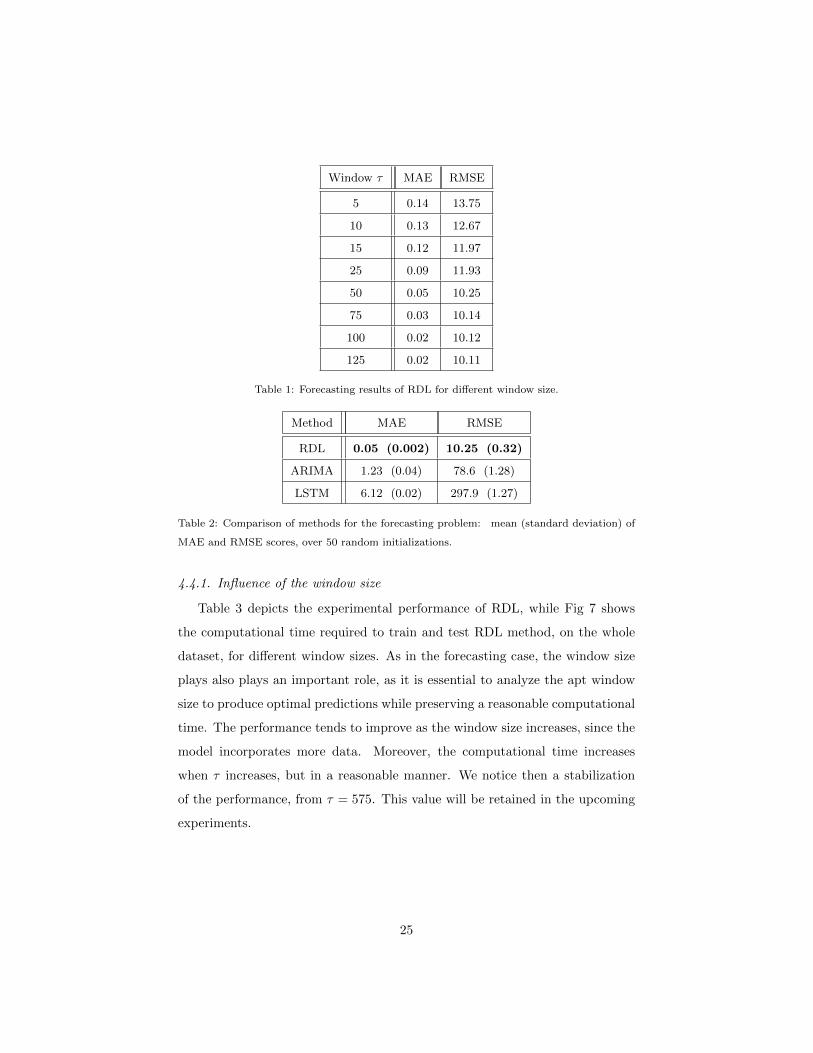
Table 1 displays the performance, in terms of MAE and RMSE, of our RDL

method when using different window size τ in the online implementation (see

Sec. 3.3.1). We can observe that the performance is improving as the window

size increases, until reaching a plateau. This trend is confirmed by Figure 4,

which illustrates the forecasting results of RDL for several values of τ , on four

representative cases. While it is clear that τ = 5, 10 or 15 may not be sufficient

2www.statsmodels.org3http://ta-lib.org4http://www.ta4j.org

21

to learn appropriately the model, we can observe that from τ = 25, the forecast-

ing results start getting satisfying. In the further experiments on forecasting,

we will set τ = 50, as it leads to a good compromise between time complexity

and prediction accuracy.

0 200 400 600 800 1000

Days

0

20

40

60

80

Ad

j. c

lose

price

Ground truth

RDL = 5

RDL = 10

RDL = 15

RDL = 25

RDL = 50

0 200 400 600 800 1000

Days

2

4

6

8

10

Ad

j. c

lose

price

Ground truth

RDL = 5

RDL = 10

RDL = 15

RDL = 25

RDL = 50

(a) (b)

0 200 400 600 800 1000

Days

-40

-20

0

20

40

Ad

j. c

lose

price

Ground truth

RDL = 5

RDL = 10

RDL = 15

RDL = 25

RDL = 50

0 200 400 600 800 1000

Days

-10

0

10

20

30

40

Ad

j. c

lose

price

Ground truth

RDL = 5

RDL = 10

RDL = 15

RDL = 25

RDL = 50

(c) (d)

Figure 4: Forecasting results of RDL method, using different values for the window size τ :

(a) AAPL, (b) ABX, (c) BAC, (d) 600841.SS. We only display here a period of 1000 days for the

sake of readibility.

4.3.2. Comparison with benchmark models

Table 2 provides the comparative performance of prediction of next day

closing price feature when using RDL, LSTM or ARIMA. It is noticeable that

RDL outperforms the two benchmark models. It is also very stable, as can be

22

0 1000 2000 3000

Days

-200

0

200

400

600

800

1000

Adj. c

lose

price

Ground truth

LSTM

ARIMA

RDL

0 1000 2000 3000

Days

-20

0

20

40

60

80

Adj. c

lose p

rice

Ground truth

LSTM

ARIMA

RDL

(a) (b)

0 1000 2000 3000

Days

0

100

200

300

Ad

j. c

lose p

rice

Ground truth

LSTM

ARIMA

RDL

0 1000 2000 3000

Days

0

500

1000

1500

Ad

j. c

lose

price

Ground truth

LSTM

ARIMA

RDL

(c) (d)

Figure 5: Forecasting results of RDL, LSTM and ARIMA models: (a) ALKYLAMINE.BO, (b)

ALOKTEXT.BO, (c) SPICEJET.BO, (d) TATASTEEL.NS.

seen in the reported standard deviation values. Note that the LSTM approach

is rather computationally expensive since it took 8 days to train for 185 stocks

for 10 years dataset, in contrast with RDL (resp. ARIMA) which requires

around 2 hours (resp. 3 hours) for the same task. Fig. 5 illustrates the closing

price prediction results, using the proposed RDL, LSTM and ARIMA method

for four representative cases. We can see that LSTM tends to underestimate

the adjusted close price. ARIMA performs well on simple cases (b-c), but has

difficulty to track the price evolution in other cases (a-d). In contrast, RDL is

23

Hold Buy SellPredicted label

Hold

Buy

Sell

True

labe

l

178564 107134 100670

13039 16984 2674

9821 7259 1854220000

40000

60000

80000

100000

120000

140000

160000

Hold Buy SellPredicted label

Hold

Buy

Sell

True

labe

l

178596 10700 100772

25753 5544 1400

21477 1182 1296320000

40000

60000

80000

100000

120000

140000

160000

(a) RDL (b) MFNN

Hold Buy SellPredicted label

Hold

Buy

Sell

True

labe

l

329899 36656 19813

27950 3356 582

21358 529 2528 50000

100000

150000

200000

250000

300000

Hold Buy SellPredicted label

Hold

Buy

Sell

True

labe

l

341969 21868 22531

30326 1689 682

22073 586 1756 50000

100000

150000

200000

250000

300000

(c) CNN-TA (d) LSTM

Figure 6: Confusion matrices for trading decision.

able to provide satisfying results in all the considered examples.

4.4. Numerical results for the trading model

We now present the results when focusing on the trading problem, that is

the prediction for the decision “hold”, ”buy” or “sell” for next day.

24

Window τ MAE RMSE

5 0.14 13.75

10 0.13 12.67

15 0.12 11.97

25 0.09 11.93

50 0.05 10.25

75 0.03 10.14

100 0.02 10.12

125 0.02 10.11

Table 1: Forecasting results of RDL for different window size.

Method MAE RMSE

RDL 0.05 (0.002) 10.25 (0.32)

ARIMA 1.23 (0.04) 78.6 (1.28)

LSTM 6.12 (0.02) 297.9 (1.27)

Table 2: Comparison of methods for the forecasting problem: mean (standard deviation) of

MAE and RMSE scores, over 50 random initializations.

4.4.1. Influence of the window size

Table 3 depicts the experimental performance of RDL, while Fig 7 shows

the computational time required to train and test RDL method, on the whole

dataset, for different window sizes. As in the forecasting case, the window size

plays also plays an important role, as it is essential to analyze the apt window

size to produce optimal predictions while preserving a reasonable computational

time. The performance tends to improve as the window size increases, since the

model incorporates more data. Moreover, the computational time increases

when τ increases, but in a reasonable manner. We notice then a stabilization

of the performance, from τ = 575. This value will be retained in the upcoming

experiments.

25

Figure 7: Time for processing the dataset (train and test), in hours, using RDL with different

window sizes τ .

Window τ Precision Recall F1 Score

Hold Sell Buy Hold Sell Buy Hold Sell Buy

25 0.85 0.10 0.10 0.85 0.12 0.12 0.84 0.10 0.10

50 0.85 0.10 0.10 0.74 0.17 0.14 0.80 0.10 0.12

75 0.85 0.10 0.10 0.74 0.18 0.15 0.78 0.11 0.12

100 0.85 0.10 0.10 0.74 0.20 0.14 0.78 0.10 0.12

200 0.85 0.10 0.09 0.68 0.25 0.22 0.72 0.13 0.14

350 0.82 0.10 0.10 0.62 0.30 0.31 0.68 0.15 0.15

575 0.88 0.15 0.12 0.45 0.52 0.51 0.59 0.19 0.23

600 0.87 0.15 0.14 0.45 0.52 0.52 0.59 0.19 0.22

Table 3: Classification results of RDL for different window sizes.

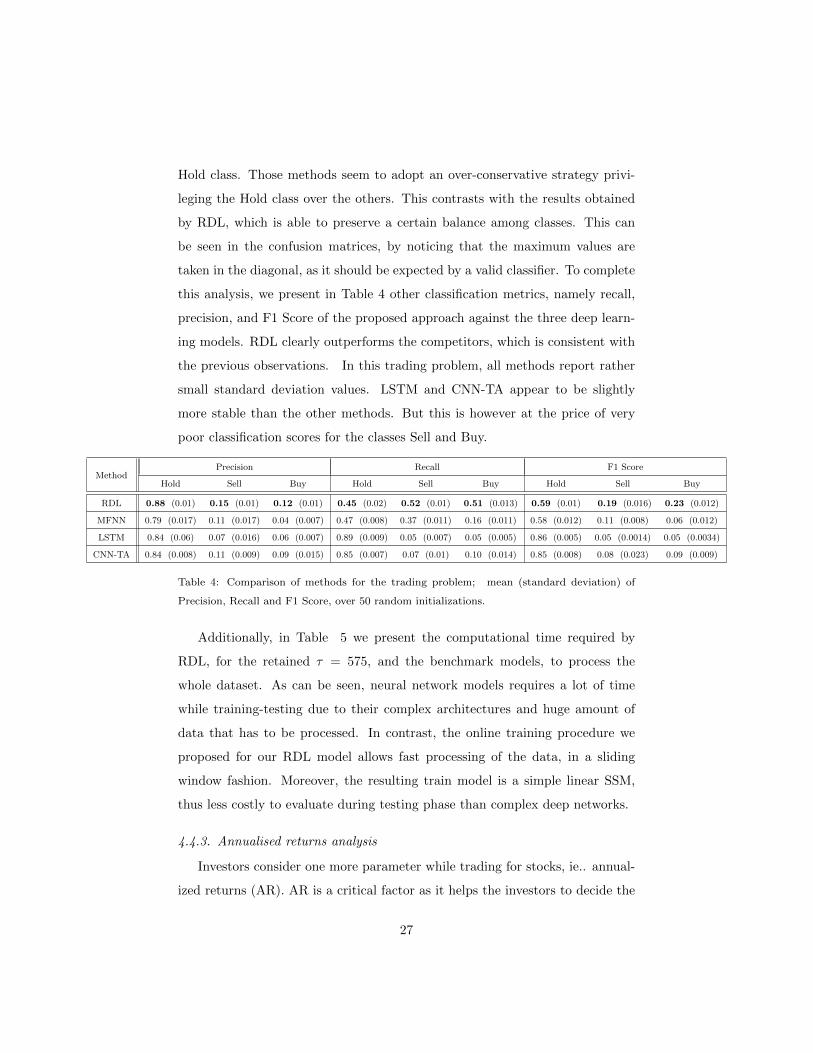
4.4.2. Classification metrics

We present in Fig. 6 the confusion matrices which summarized the classifi-

cation performance for the 185 stocks by the proposed approach, as well as for

the three competitors. First, we see that for all the approaches, the Hold class

is better predicted than the two other classes, LSTM getting the best scores

over the competitors in terms of false negative. However, LSTM (and to a mild

extent, CNN-TA and MFNN) present a large number of false positive for the

26

Hold class. Those methods seem to adopt an over-conservative strategy privi-

leging the Hold class over the others. This contrasts with the results obtained

by RDL, which is able to preserve a certain balance among classes. This can

be seen in the confusion matrices, by noticing that the maximum values are

taken in the diagonal, as it should be expected by a valid classifier. To complete

this analysis, we present in Table 4 other classification metrics, namely recall,

precision, and F1 Score of the proposed approach against the three deep learn-

ing models. RDL clearly outperforms the competitors, which is consistent with

the previous observations. In this trading problem, all methods report rather

small standard deviation values. LSTM and CNN-TA appear to be slightly

more stable than the other methods. But this is however at the price of very

poor classification scores for the classes Sell and Buy.

MethodPrecision Recall F1 Score

Hold Sell Buy Hold Sell Buy Hold Sell Buy

RDL 0.88 (0.01) 0.15 (0.01) 0.12 (0.01) 0.45 (0.02) 0.52 (0.01) 0.51 (0.013) 0.59 (0.01) 0.19 (0.016) 0.23 (0.012)

MFNN 0.79 (0.017) 0.11 (0.017) 0.04 (0.007) 0.47 (0.008) 0.37 (0.011) 0.16 (0.011) 0.58 (0.012) 0.11 (0.008) 0.06 (0.012)

LSTM 0.84 (0.06) 0.07 (0.016) 0.06 (0.007) 0.89 (0.009) 0.05 (0.007) 0.05 (0.005) 0.86 (0.005) 0.05 (0.0014) 0.05 (0.0034)

CNN-TA 0.84 (0.008) 0.11 (0.009) 0.09 (0.015) 0.85 (0.007) 0.07 (0.01) 0.10 (0.014) 0.85 (0.008) 0.08 (0.023) 0.09 (0.009)

Table 4: Comparison of methods for the trading problem; mean (standard deviation) of

Precision, Recall and F1 Score, over 50 random initializations.

Additionally, in Table 5 we present the computational time required by

RDL, for the retained τ = 575, and the benchmark models, to process the

whole dataset. As can be seen, neural network models requires a lot of time

while training-testing due to their complex architectures and huge amount of

data that has to be processed. In contrast, the online training procedure we

proposed for our RDL model allows fast processing of the data, in a sliding

window fashion. Moreover, the resulting train model is a simple linear SSM,

thus less costly to evaluate during testing phase than complex deep networks.

4.4.3. Annualised returns analysis

Investors consider one more parameter while trading for stocks, ie.. annual-

ized returns (AR). AR is a critical factor as it helps the investors to decide the

27

Method Time cost (h.)

RDL 2.34

MFNN 3.87

LSTM 9.5

CNN-TA 7.54

Table 5: Averaged time over 50 random runs for processing the dataset (train and test), in

hours, for RDL and its competitors.

monetary gain/loss they are going to incur while investing in the stock. The

predictions (buy, sell, hold) provided by the model are then used to carry out

the market simulation where a similar virtual environment is created by buying,

selling, and holding the stock as per the predictions. The market simulations

are a strategy that mimics the investor/trader who makes trading decisions ac-

cording to signals from the algorithmic model using real money, which then

allows to compute AR. Table 6 presents the AR results obtained when applying

the market simulations strategy from [99], to the trading predictions provided

by our proposed model and the other benchmark techniques, on 9 randomly

selected stocks, as well as the average AR for all stocks. The best-annualized

returns are highlighted in bold. One can notice that the proposed method leads

to higher returns in averaged during the test period of 10 years when compared

to AR obtained using the trading predictions from the deep learning techniques.

4.4.4. Portfolio diversification

Many investment professionals claim that the key to smart trading is ”diver-

sification of portfolio” [97]. Diversification allows investors to maximize returns

by investing in different domains that would react differently in the same market

events, thus managing better the risk. Ideally, a diversified portfolio would con-

tain stocks with various levels of market capitalization. Market capitalization

refers to the total market value of all outstanding shares [98]. Companies can be

divided according to their market capitalization value, into small-cap, mid-cap,

large-cap, as we will explain hereafter in detail. It is always beneficial to have

28

Stock symbols RDL CNN-TA MFNN LSTM

WIPRO.BO 1.37 -18.14 -27.81 -47.74

AAPL 13.44 0 12.92 0

AMZN 0.06 30.64 -20.85 -0.15

IOC.BO 6.28 -3.03 -26.42 -3.1

TATACHEM.BO 3.91 -1.54 -8.32 0

SPICEJET.BO 10.58 -24.08 -28.21 0

ATML 3.76 -33.25 -27.07 -33.82

DOM.L 1.76 0.11 8.22 0.47

INDRAMEDCO.BO 5.61 -14.22 -3.53 -50.86

Average on all 185 stocks 5.19 -5.08 -11.45 -13.02

Table 6: Annualized Returns

Stock symbols Log-Loss

Sm

all-

cap

ALOKTEXT.BO 1.11

ALKYLAMINE.BO 1.22

ZEEMEDIA6.BO 1.03

PVP.BO 0.42

Mid

-cap

IOC.BO 1.25

TATACHEM.BO 0.56

SPICEJET.BO 0.47

BHEL.BO 0.01

Lar

ge-c

ap

AAPL 0.85

AMZN 0.27

HINDZINC.BO 1.03

ONGC.BO 0.007

SIEMENS.NS 0.001

Table 7: Log-loss values provided by RDL, for the stocks with available market capitalization

categories.

29

a diversified portfolio that includes stocks from the three classes of companies.

Small-cap companies are young and seek to expand aggressively. As comes the

growth potential, the risk factor follows in a direct proportion. Small-caps are

more volatile and vulnerable to losses during the negative trends (downtime) of

the financial market.

Mid-cap is a pooled investment that focuses on including stocks with a middle

range of market capitalization. Mid-cap offers investors more enormous growth

potential than large-cap stocks, but with less volatility and risk as compared to

small-caps.

Large-cap companies are typically large, well established, and financially sound.

Large-cap is the market leader, relatively less volatile, and has a steady risk-

return factor with relatively lower risk compared to mid-cap, small-cap.

As explained in Sec. 3.3.3, the proposed RDL methodology allows to provide

through probabilistic quantification, a piece of information that can be used by

a knowledgeable practitioner to trade accordingly to have a diversified portfolio.

Such probabilistic validation can help maximize the returns by having a mix of

small-cap, mid-cap, large-cap stocks.

We provide in Table 7 the log-loss value (the smaller, the better), computed

as described in Sec. 3.3.3, computed for RDL results, for the few stocks of

the dataset for which the market capitalization categories were available.5 The

log-loss quantifies the accuracy of the probabilistic predictions of the proposed

method, penalizing more the situations where the method assigns a low proba-

bility to an event that finally occurs. One can notice that the log-loss value can

reach very low value (i.e., good prediction accuracy) when trading the large cap

stocks, probably due to the less volatile nature of such stocks. In contrast, the

log-loss is in average higher for small caps, as they are highly volatile.

4.4.5. Result Discussion

One importance difference between RDL and the competitors is that our

5https://finance.yahoo.com/screener

30

approach is not supervised, in the sense that we do not need to load a long

time series to learn the model in a batch manner. Therfore, RDL processes

data as it comes and in a sequential manner. This is convenient in terms of

memory and processing cost. This perspective helps to explain the good results

of RDL, as it always uses all available information to make a one day ahead

prediction, while keeping a low complexity. The challenge for RDL, that we

also tackle in this paper, is to adequately learn the linear matrices of the model

from small time windows (maximum 600 days in our tests), and jointly, per-

form the forecasting. The efficient learning and prediction tasks are supported

by Kalman filter/smoother combined with the EM. The flexibility of RDL, with

potentially different linear operators along time (the linear operators are up-

dated from a window to the next one), is beneficial to model non-linear and

non-stationary time series. Moreover, the Gaussian linear SSM yields simple

updates for the EM, reducing considerably the ‘training’ time. In contrast, if we

trained the benchmark models, on each small sliding window, it would be very

costly, and most likely with a reduced performance (the models would be over-

parametrized). Under this perspective, we can consider that RDL deals with a

piece-wise linear state-space model with smooth changes of the linear operators

(that are estimated over time), while still retaining the linear-Gaussian structure

which allows to extract all the benefits of the Kalman filtering/smoothing.

5. Conclusion

We have proposed a new tool, called RDL, for dynamical modelling and pre-

dicting financial time series. Our method has the ability to provide theoretically

sought state inference along with uncertainty estimation. It also includes an it-

erative model estimation mechanism relying on an expectation-minimization

methodology. We provide an online version of such estimation method based

on a sliding window approach. Results show that our method achieves better

results than state-of-the-art models that are tailored for the problems of stock

forecasting and stock trading.

31

The proposed RDL approach relies on a linear state-space model on the

observed features, with linear Markovian relationship between two consecutive

hidden states. In future work, we aim to come up with a more sophisticated

model including non-linear activation functions.

6. Acknowlegdment

This work was supported by the CNRS-CEFIPRA project under grant NextGenBP

PRC2017.

References

[1] D. Shah, H. Isah, F. Zulkernine, Stock market analysis: A review and tax-

onomy of prediction techniques, International Journal of Financial Studies

7 (2) (2019) 26.

[2] E. Fama, Random walks in stock market prices, Financial Analysts Jour-

nal 51 (1) (1995) 75–80.

[3] B. Malkiel, E. Fama, Efficient capital markets: A review of theory and

empirical work, The journal of Finance 25 (2) (1970) 383–417.

[4] Y. Kwon, B. Moon, A hybrid neurogenetic approach for stock forecasting,

IEEE Transactions on Neural Networks 18 (3) (2007) 851–864.

[5] G. Atsalakis, K. Valavanis, Surveying stock market forecasting

techniques–part ii: Soft computing methods, Expert Systems with Ap-

plications 36 (3) (2009) 5932–5941.

[6] P. Pai, C. Lin, A hybrid arima and support vector machines model in

stock price forecasting, Omega 33 (6) (2005) 497–505.

[7] G. Box, G. Tiao, Intervention analysis with applications to economic and

environmental problems, Journal of the American Statistical Association

70 (349) (1975) 70–79.

32

[8] A. Pankratz, Forecasting with dynamic regression models, Vol. 935, John

Wiley & Sons, 2012.

[9] R. Hyndman, A. Koehler, J. Ord, R. Snyder, Forecasting with exponential

smoothing: the state space approach, Springer Science & Business Media,

2008.

[10] G. Pandher, Forecasting multivariate time series with linear restrictions

using constrained structural state-space models, Journal of Forecasting

21 (4) (2002) 281–300.

[11] J. McCarthy, M. Najand, State space modeling of price and volume de-

pendence: evidence from currency futures, Journal of Futures Markets

13 (4) (1993) 335–344.

[12] J. Ng, C. Forbes, G. Martin, B. McCabe, Non-parametric estimation of

forecast distributions in non-gaussian, non-linear state space models, In-

ternational Journal of Forecasting 29 (3) (2013) 411–430.

[13] N. Shephard, Partial non-Gaussian state space, Biometrika 81 (1) (1994)

115–131.

[14] S. Sarkka, Bayesian Filtering and Smoothing, 3rd Edition, 2013.

[15] A. Harvey, Forecasting, structural time series models and the Kalman

filter, 1990.

[16] R. Handa, A. Shrivas, H. Hota, Financial time series forecasting using

back propagation neural network and deep learning architecture, Int. J.

Recent Technol. Eng 8 (2019) 3487–3492.

[17] X. Zhang, X. Liang, A. Zhiyuli, S. Zhang, R. Xu, B. Wu, At-lstm: An

attention-based lstm model for financial time series prediction, in: IOP

Conference Series: Materials Science and Engineering, Vol. 569, IOP Pub-

lishing, 2019, p. 052037.

33

[18] Y. Huang, Y. Gao, Y. Gan, M. Ye, A new financial data forecasting model

using genetic algorithm and long short-term memory network, Neurocom-

puting (2020).

[19] R. Li, K. W. Fong, S.C, Forecasting the reits and stock indices: group

method of data handling neural network approach, Pacific Rim Property

Research Journal 23 (2) (2017) 123–160.

[20] K. Ho, W. Wang, Predicting stock price movements with news sentiment:

An artificial neural network approach, in: Artificial Neural Network Mod-

elling, Springer, 2016, pp. 395–403.

[21] S. Hochreiter, J. Schmidhuber, Long short-term memory, Neural Compu-

tation 9 (8) (1997) 1735–1780.

[22] J. Chung, C. Gulcehre, K. Cho, Y. Bengio, Empirical evaluation of gated

recurrent neural networks on sequence modeling, Tech. rep., https://

arxiv.org/abs/1412.3555 (2014).

[23] I. Tosic, P. Frossard, Dictionary learning: What is the right representation

for my signal?, IEEE Signal Processing Magazine 28 (2011) 27–38.

[24] A. A. Ariyo, A. Adewumi, C. Ayo, Stock price prediction using the

ARIMA model, in: Proceedings of the 16th International Conference on

Computer Modelling and Simulation, IEEE, 2014, pp. 106–112.

[25] P. Mondal, L. Shit, S. Goswami, Study of effectiveness of time series

modeling (ARIMA) in forecasting stock prices, International Journal of

Computer Science, Engineering and Applications 4 (2) (2014) 13.

[26] J. Jarrett, E. Kyper, ARIMA modeling with intervention to forecast and

analyze chinese stock prices, International Journal of Engineering Business

Management 3 (3) (2011) 53–58.

[27] B. Devi, D. Sundar, P. Alli, An effective time series analysis for stock

trend prediction using ARIMA model for nifty midcap-50, International

34

Journal of Data Mining & Knowledge Management Process 3 (1) (2013)

65.

[28] A. Petrica, S. Stancu, A. Tindeche, Limitation of ARIMA models in finan-

cial and monetary economics., Theoretical & Applied Economics 23 (4)

(2016).

[29] S. Makridakis, M. Hibon, Arma models and the box–jenkins methodology,

Journal of Forecasting 16 (3) (1997) 147–163.

[30] T. M. O’Donovan, Short term forecasting: An introduction to the Box-

Jenkins approach., JOHN WILEY & SONS, 1983.

[31] S. Chadsuthi, C. Modchang, Y. Lenbury, S. Iamsirithaworn, W. Triampo,

Modeling seasonal leptospirosis transmission and its association with rain-

fall and temperature in thailand using time–series and arimax analyses,

Asian Pacific Journal of Tropical Medicine 5 (7) (2012) 539–546.

[32] R. Kalman, A new approach to linear filtering and prediction problems

(1960).

[33] J. P. Nobrega, A. L. O., A sequential learning method with Kalman filter

and extreme learning machine for regression and time series forecasting,

Neurocomputing 337 (2019) 235–250.

[34] N. Saini, A. Mittal, Forecasting volatility in indian stock market using

state space models, Journal of Statistical and Econometric Methods 3 (1)

(2014) 115–136.

[35] Y. Zeng, S. Wu, State-space models: Applications in economics and fi-

nance, Vol. 1, Springer, 2013.

[36] E. Zivot, J. Wang, S. Koopman, State space modelling in macroeconomics

and finance using ssfpack in s+ finmetrics, State Space and Unobserved

Component Models (2004) 284–335.

35

[37] L. Ljung, Asymptotic behavior of the extended Kalman filter as a pa-

rameter estimator for linear systems, IEEE Transactions on Automatic

Control 24 (1) (1979) 36–50.

[38] C. Slim, Neuro-fuzzy network based on extended kalman filtering for finan-

cial time series, World Academy of Science, Engineering and Technology

22 (2006) 134–139.

[39] E. Wan, R. Van Der Merwe, The unscented kalman filter for nonlinear

estimation, in: Proceedings of the IEEE Adaptive Systems for Signal

Processing, Communications, and Control Symposium, IEEE, 2000, pp.

153–158.

[40] D. Crisan, A. Doucet, A survey of convergence results on particle filtering

methods for practitioners, IEEE Transactions on Signal Processing 50 (3)

(2002) 736–746.

[41] P. Djuric, J. Kotecha, J. Zhang, Y. Huang, T. Ghirmai, M. Bugallo,

J. Miguez, Particle filtering, IEEE Signal Processing Magazine 20 (5)

(2003) 19–38.

[42] A. Doucet, A. M. Johansen, A tutorial on particle filtering and smoothing:

Fifteen years later, Handbook of nonlinear filtering 12 (656-704) (2009) 3.

[43] R. Casarin, C. Trecroci, et al., Business cycle and stock market volatility:

A particle filter approach, Universita degli studi, Dipartimento di scienze

economiche, 2006.

[44] A. Javaheri, D. Lautier, A. Galli, Filtering in finance, Wilmott 3 (2003)

67–83.

[45] J. Smith, A. Santos, Second-order filter distribution approximations for fi-

nancial time series with extreme outliers, Journal of Business & Economic

Statistics 24 (3) (2006) 329–337.

36

[46] V. Elvira, L. Martino, M. F. Bugallo, P. Djuric, In search for improved

auxiliary particle filters, in: Signal Processing Conference (EUSIPCO),

2018 Proceedings of the 26th European, IEEE, 2018, pp. 1–5.

[47] V. Elvira, L. Martino, M. F. Bugallo, P. M. Djuric, Elucidating the auxil-

iary particle filter via multiple importance sampling [lecture notes], IEEE

Signal Processing Magazine 36 (6) (2019) 145–152.

[48] V. Elvira, J. Mıguez, P. Djuric, Adapting the number of particles in se-

quential monte carlo methods through an online scheme for convergence

assessment, IEEE Transactions on Signal Processing 65 (7) (2017) 1781–

1794.

[49] V. Elvira, J. Mıguez, P. Djuric, New results on particle filters with adap-

tive number of particles, arXiv preprint arXiv:1911.01383 (2017).

[50] A. Harvey, Forecasting, structural time series models and the Kalman

filter, 1990.

[51] M. Eichler, Graphical modelling of multivariate time series, Probabil-

ity Theory and Related Fields 153 (1) (2012) 233–268. doi:10.1007/

s00440-011-0345-8.

URL https://doi.org/10.1007/s00440-011-0345-8

[52] F. R. Bach, M. I. Jordan, Learning graphical models for stationary time

series, IEEE Transactions on Signal Processing 52 (8) (2004) 2189–2199.

doi:10.1109/TSP.2004.831032.

[53] D. Barber, A. T. Cemgil, Graphical models for time-series, IEEE Sig-

nal Processing Magazine 27 (6) (2010) 18–28. doi:10.1109/MSP.2010.

938028.

[54] E. Chouzenoux, V. Elvira, GraphEM: EM algorithm for blind Kalman

filtering under graphical sparsity constraints, in: Proceedings of the IEEE

International Conference on Acoustics, Speech and Signal Processing

(ICASSP 2020), 2020, pp. 1–5.

37

[55] M. Abe, H. Nakayama, Deep learning for forecasting stock returns in the

cross-section, in: Proceedings of the Pacific-Asia Conference on Knowl-

edge Discovery and Data Mining, Springer, 2018, pp. 273–284.

[56] R. Singh, S. Srivastava, Stock prediction using deep learning, Multimedia

Tools and Applications 76 (18) (2017) 18569–18584.

[57] D. Lien Minh, A. Sadeghi-Niaraki, H. D. Huy, K. Min, H. Moon, Deep

learning approach for short-term stock trends prediction based on two-

stream gated recurrent unit network, IEEE Access 6 (2018) 55392–55404.

[58] Y. Xu, S. Cohen, Stock movement prediction from tweets and historical

prices, in: Proceedings of the 56th Annual Meeting of the Association for

Computational Linguistics, Vol. 1, 2018, pp. 1970–1979.

[59] Z. Hu, W. Liu, J. Bian, X. Liu, T. Liu, Listening to chaotic whispers:

A deep learning framework for news-oriented stock trend prediction, in:

Proceedings of the 11th ACM International Conference on Web Search

and Data Mining, ACM, 2018, pp. 261–269.

[60] G. Zhang, Neural Networks in Business Forecasting, Vol. 6 of IGI Global.

Journal of Intelligent Systems, 2004.

[61] H. Kim, K. Shin, A hybrid approach based on neural networks and genetic

algorithms for detecting temporal patterns in stock markets, Applied Soft

Computing 7 (2) (2007) 569–576.

[62] M. R. Hassan, A combination of hidden Markov model and fuzzy model for

stock market forecasting, Neurocomputing 72 (16-18) (2009) 3439–3446.

[63] X. Zhong, D. Enke, A comprehensive cluster and classification mining

procedure for daily stock market return forecasting, Neurocomputing 267

(2017) 152–168.

[64] M. Hiransha, E. Gopalakrishnan, V. K. Menon, K. Soman, NSE stock

market prediction using deep-learning models, Procedia Computer Science

132 (2018) 1351–1362.

38

[65] M. Kumar, M. Thenmozhi, Forecasting stock index returns using ARIMA-

SVM, ARIMA-ANN, and ARIMA-random forest hybrid models, Interna-

tional Journal of Banking, Accounting and Finance 5 (3) (2014) 284–308.

[66] X. Ding, Y. Zhang, T. Liu, J. Duan, Deep learning for event-driven stock

prediction, in: Proceedings of the 24th International Joint Conference on

Artificial Intelligence (IJCAI 2015), 2015.

[67] R. Akita, A. Yoshihara, T. Matsubara, K. Uehara, Deep learning for stock

prediction using numerical and textual information, in: Proceedings of

the 15th International Conference on Computer and Information Science

(ICIS 2016), IEEE, 2016, pp. 1–6.

[68] E. Chong, C. Han, F. Park, Deep learning networks for stock market anal-

ysis and prediction: Methodology, data representations, and case studies,

Expert Systems with Applications 83 (2017) 187–205.

[69] T. Fischer, C. Krauss, Deep learning with long short-term memory net-

works for financial market predictions, European Journal of Operational

Research 270 (2) (2018) 654–669.

[70] T. Gao, Y. Chai, Improving stock closing price prediction using recur-

rent neural network and technical indicators, Neural Computation 30 (10)

(2018) 2833–2854.

[71] Z. Che, S. Purushotham, K. Cho, D. Sontag, Y. Liu, Recurrent neural net-

works for multivariate time series with missing values, Scientific Reports

8 (1) (2018) 1–12.

[72] M. Schuster, K. Paliwal, Bidirectional recurrent neural networks, IEEE

Transactions on Signal Processing 45 (11) (1997) 2673–2681.

[73] D. E. Rumelhart, G. E. Hinton, R. J. Williams, Learning Internal Repre-

sentations by Error Propagation, MIT Press, Cambridge, MA, USA, 1986,

p. 318–362.

39

[74] D. Nelson, A. Pereira, R. de Oliveira, Stock market’s price movement

prediction with LSTM neural networks, in: Proceedings of the Interna-

tional Joint Conference on Neural Networks (IJCNN 2017), IEEE, 2017,

pp. 1419–1426.

[75] A. Samarawickrama, T. Fernando, A recurrent neural network approach in

predicting daily stock prices an application to the Sri Lankan stock market,

in: Proceedings of the IEEE International Conference on Industrial and

Information Systems (ICIIS 2017), 2017, pp. 1–6.

[76] Z. Shen, Y. Zhang, J. Lu, J. Xu, G. Xiao, A novel time series forecasting

model with deep learning, Neurocomputing 396 (2020) 302–313.

[77] R. Fu, Z. Zhang, L. Li, Using LSTM and GRU neural network methods

for traffic flow prediction, in: Proceedings of the 31st Youth Academic

Annual Conference of Chinese Association of Automation (YAC 2016),

IEEE, 2016, pp. 324–328.

[78] Y. Li, Z. Zhu, D. Kong, H. Han, Y. Zhao, Ea-lstm: Evolutionary attention-

based lstm for time series prediction, Knowledge-Based Systems 181

(2019) 104785.

[79] K. Althelaya, E. El-Alfy, S. Mohammed, Evaluation of bidirectional LSTM

for short-and long-term stock market prediction, in: Proceedings of the

9th international conference on information and communication systems

(ICICS 2018), IEEE, 2018, pp. 151–156.

[80] Y. Hua, Z. Zhao, R. Li, X. Chen, Z. Liu, H. Zhang, Deep learning with

long short-term memory for time series prediction, IEEE Communications

Magazine 57 (6) (2019) 114–119.

[81] S. Kiranyaz, T. Ince, M. Gabbouj, Real-time patient-specific ECG clas-

sification by 1-d convolutional neural networks, IEEE Transactions on

Biomedical Engineering 63 (3) (2015) 664–675.

40

[82] K. Kashiparekh, J. Narwariya, P. Malhotra, L. Vig, G. Shroff, Con-

vtimenet: A pre-trained deep convolutional neural network for time series

classification, in: Proceedings of the International Joint Conference on

Neural Networks (IJCNN 2019), IEEE, 2019, pp. 1–8.

[83] D. Smirnov, E. Nguifo, Time series classification with recurrent neural

networks, Advanced Analytics and Learning on Temporal Data (2018) 8.

[84] E. Abbe, C. Sandon, Provable limitations of deep learning, arXiv preprint

arXiv:1812.06369 (2018).

[85] J. Mairal, F. Bach, J. Ponce, G. Sapiro, Online learning for matrix factor-

ization and sparse coding., Journal of Machine Learning Research 11 (1)

(2010).

[86] X. Li, H. Shen, L. Zhang, H. Zhang, Q. Yuan, G. Yang, Recovering quan-

titative remote sensing products contaminated by thick clouds and shad-

ows using multitemporal dictionary learning, IEEE Transactions on Geo-

science and Remote Sensing 52 (11) (2014) 7086–7098.

[87] J. Mairal, F. Bach, J. Ponce, Task-driven dictionary learning, IEEE trans-

actions on pattern analysis and machine intelligence 34 (4) (2011) 791–804.

[88] Y. Xu, Z. Li, J. Yang, D. Zhang, A survey of dictionary learning algorithms

for face recognition, IEEE access 5 (2017) 8502–8514.

[89] Y. Xu, Z. Li, B. Zhang, J. Yang, J. You, Sample diversity, representation

effectiveness and robust dictionary learning for face recognition, Informa-

tion Sciences 375 (2017) 171–182.

[90] Z. Li, Z. Lai, Y. Xu, J. Yang, D. Zhang, A locality-constrained and label

embedding dictionary learning algorithm for image classification, IEEE

transactions on neural networks and learning systems 28 (2) (2015) 278–

293.

41

[91] R. H. Shumway, D. S. Stoffer, An approach to time series smoothing and

forecasting using the EM algorithm, Journal of Time Series Analysis 3 (4)

(1982) 253–264.

[92] P. Gupta, J. Maggu, A. Majumdar, E. Chouzenoux, G. Chierchia, Decon-

fuse: a deep convolutional transform-based unsupervised fusion frame-

work, EURASIP Journal on Advances in Signal Processing (1) (2020)

1–32.

[93] M. Pereyra, P. Schniter, E. Chouzenoux, J.-C. Pesquet, J. Tourneret,

A. Hero, S. McLaughlin, A survey of stochastic simulation and optimiza-

tion methods in signal processing, IEEE Journal of Selected Topics in

Signal Processing 10 (2) (2016) 224–241.

[94] C. F. J. Wu, On the convergence properties of the EM algorithm, The

Annals of Statistics 11 (1) (1983) 95–103.

[95] E. Chouzenoux, A. Jezierska, J. Pesquet, H. Talbot, A majorize-minimize

subspace approach for l2-l0 image regularization, SIAM Journal on Imag-

ing Science 6 (1) (2013) 563–591.

[96] E. Chouzenoux, J. Pesquet, A stochastic majorize-minimize subspace al-

gorithm for online penalized least squares estimation, IEEE Transactions

on Signal Processing 65 (18) (2017) 4770–4783.

[97] S. Griffith-Jones, M. Segoviano, S. Spratt, Basel II and developing coun-

tries: diversification and portfolio effects, Tech. Rep. 34, LSE Financial

Markets Group, discussion paper 437 (2003).

[98] V. Kumar, D. Shah, Expanding the role of marketing: from customer

equity to market capitalization, Journal of Marketing 73 (6) (2009) 119–

136.

[99] O. Sezer, A. Ozbayoglu, Algorithmic financial trading with deep convolu-

tional neural networks: Time series to image conversion approach, Applied

Soft Computing 70 (2018) 525–538.

42

[100] W. Long, Z. Lu, L. Cui, Deep learning-based feature engineering for stock

price movement prediction, Knowledge-Based Systems 164 (2019) 163–

173.

43