Recovery of disruptions in rapid transit networks Luis Cadarso3'*, Angel Marin3, Gabor Marotib

a Universidad Politecnica de Madrid, Escuela Tecnica Superior de Ingenieros Aeronauticos, Plaza Cardenal Cisneros, 3, 28040 Madrid, Spain b Process Quality and Innovation, Netherlands Railways, 3500 HA, Utrecht, Netherlands

A B S T R A C T

This paper studies the disruption management problem of rapid transit rail networks. Besides optimizing the timetable and the rolling stock schedules, we explicitly deal with the effects of the disruption on the passenger demand.

We propose a two-step approach that combines an integrated optimization model (for the timetable and rolling stock) with a model for the passengers' behavior.

We report our computational tests on realistic problem instances of the Spanish rail operator RENFE. The proposed approach is able to find solutions with a very good balance between various managerial goals within a few minutes.

1. Introduction

During the daily operations of a dense railway network, incidents may cause the railway traffic to deviate from the planned operations. These incidents may make it impossible to operate the schedule as it was originally planned. In such a situation the operator needs to adjust the timetable and the rolling stock assignment for the time interval of the incident, and to carry out further recovery steps in order to get back to the original schedules.

The first task after noticing an incident is to determine whether or not it requires a substantial active intervention. If it does, the railway operations are said to be disrupted, and plans must be designed in order to recover from the disrupted sit­uation. Disruptions may be caused by infrastructure blockage, failing rolling stock, and crew shortage. On the other hand, small-scale incidents appear in case of minor train delays; they are resolved by letting the delays propagate until the time­table's buffer times absorb them. A recent summary of causes of disruptions is given by Nielsen (2011). Note that the dis­tinction between small incidents and large disruptions is practice-driven.

Regardless of the cause of a disruption, it has an impact on the railway system. The impact is generally in the form of a change in the system settings, a change in resource availability, or both. Disruptions usually involve a change in resource availability. The response to a change in resource availability is to replan the current operations to apply only the available resources which may include giving up some of the planned services. A disruption may also cause a change in the system settings. Closing a station (or part thereof) temporarily is an example of a change in the system settings that affects the sys­tem's ability to operate.

A further change in the system environment is a deviation in demand because the passengers are free to choose their own path in the network. In case of a disruption, some paths will not be available anymore and others may become less attractive. Passengers react to disruptions in different ways: either they reroute themselves, or they wait for a train in their original

* Corresponding author. E-mail addresses: luis.cadarso@upm.es (L. Cadarso), angel.marin@upm.es (A. Marin), gabor.maroti@ns.nl (G. Maroti).

path, or they choose a different mode of transport, or they do not travel at all. Such a situation would require to pay an addi­tional economic cost for the passenger.

A particularly challenging aspect of disruption management is the fact that the passenger demand is influenced by the operator's recovery actions, too. Timetabling decisions may cancel traveling options, or insert additional ones, while the roll­ing stock decisions influence the capacity of the trains. The actual passenger flows emerge from the interaction of the time­table, the rolling stock schedule and the passengers.

In the current railway practice, the recovery problem is solved in a sequential manner. When a disruption occurs, first a new timetable is computed accounting for rolling stock availability; as a result, the rolling stock units will not finish their daily duties at the location where they were planned to: to avoid deadheading trips, the rolling stock schedules are modified such that the rolling stock is balanced before the end of the day. However, this approach has limitations: computing a new timetable without accounting for rolling stock may produce a suboptimal timetable or even an infeasible one for rolling stock assignment purposes. Therefore, we are interested in an integrated approach to obtain an optimal solution for timetable and rolling stock assignment accounting for demand rerouting.

To produce recovery plans is a complex task since the presented resources have to be re-planned in real-time. A compli­cating issue in a disrupted situation is the fact that the duration of the disruption is usually not known exactly and that the status of the railway system is changing at the same time. As a consequence, the dispatchers apply rescheduling actions sev­eral times, always taking the latest available information into account.

The disruption management process has several objectives. The first goal is to provide the best possible service quality by accommodating the largest possible part of passenger demand. The second goal aims at easing the rescheduling process itself by minimizing the differences between the original (undisrupted) plan and the recovery plan. Third, the operators often want to quickly return to the original plan once the disruption is over. That is, the duration of the recovery period is to be minimized.

This paper is organized as follows. In Section 2 a literature overview and paper contributions are given. Section 3 de­scribes the problem in detail. Section 4 is devoted to the mathematical model. In Section 5 we present our computational experiments. Finally, we draw some conclusions in Section 6.

2. State of art

Jespersen-Groth et al. (2009) deal with disruption management in passenger railway transportation. They describe the disruption management process and the roles of the different actors involved in it. Furthermore, they discuss the three main subproblems in railway disruption management: timetable adjustment, and rolling stock and crew re-scheduling, de Almei­da et al. (2003) propose an approach for dealing with large scale disruptions where track capacity is greatly reduced. As once a disruption has occurred, the first dispatching task is to keep the railway system running, the first decisions are taken under extreme time pressure. Therefore, decision proposals should be generated quickly. Thus, they propose a heuristic approach to re-building a passenger transportation plan in real time. Kroon and Huisman (2011) also state that, in case of a disruption, rescheduling is a time critical situation where every minute counts. They describe models and algorithms for real-time roll­ing stock rescheduling and real-time crew rescheduling.

During a disruption, the dispatchers try to use all available rolling stock to transport as many passengers as possible in the right direction. As a result, the rolling stock units will not finish their daily duties at the location where they were planned to. Budai et al. (2010) state that in order to prevent expensive deadheading trips, it is attractive to modify the rolling stock schedules such that the rolling stock is balanced before the night.

Nielsen (2011) studies the rescheduling of passenger railway rolling stock in disruption management and in the short-term planning phase. He formalizes the rolling stock rescheduling problem as a heuristic approach that uses three steps. The first step creates a rolling stock schedule based on the current timetable and passenger demand. The second step sim­ulates the passenger response, and the third step interprets the passenger response. All test instances are based on the major Dutch railway operator NS.

Walker et al. (2005) are among the first ones to deal with the integration of timetabling and resource scheduling in dis­ruption management. They present a model that manipulates the timetable and the crew schedule at the same time. The objective is to simultaneously minimize the deviation of the new timetable from the original one, and the cost of the crew schedule.

Cacchiani et al. (2012) describe a two-stage optimization model for determining robust rolling stock circulations for pas­senger trains. Here robustness means that the rolling stock circulations can better deal with large disruptions of the railway system. These large disruptions are given by a number of scenarios. They measure lack of rolling stock capacity based on a given anticipated passenger demand and state that minimizing the number of canceled trips limits the passenger inconve­nience. They evaluate their approach on the real-life rolling stock-planning problem of NS.

In the airline industry, the recoverability of the system from disruptions has been studied deeper. Clausen (2007) gives a short overview over the methods used for planning and disruption management in the airline industry. Then he describes and discusses the situation regarding railway optimization.

It is also current practice to determine recovery plans in a primarily sequential manner, first recovering aircraft, then crew, and then passengers (Filar et al., 2000). With respect to aircraft recovery, Jarrah et al. (1993) consider the aircraft sche-

dule recovery problem and propose two network models to address aircraft shortages. The objective of the first model is to determine flight leg departure times that minimize total flight delay costs, and the second is to select flight leg cancellations that minimize cancellation costs. Thengvall et al. (1998) extend the approach of Jarrah et al. (1993) to consider flight leg departure scheduling and cancellations simultaneously. Rosenberger et al. (2003) present an optimization model that reschedules legs and reroutes aircraft by minimizing an objective function involving rerouting and cancellation costs. Then, they revise the model to minimize crew and passenger disruptions. Stojkovic et al. (2002) propose a model to select flight leg departure times, considering crew transfers, rest periods, passenger connections, and aircraft maintenance, but not including cancellation decisions.

Bratu and Barnhart (2006) present airline schedule recovery models and algorithms that simultaneously develop recovery plans for aircraft, crews, and passengers by determining which flight leg departures to postpone and which to cancel. The objective is to minimize jointly airline operating costs, estimated passenger delay and disruption costs. Dumas and Soumis (2008) and Dumas et al. (2009) propose a framework for revenue management where aircrarft scheduling is combined with a passenger flow model.

The main difference between the airline and railway settings is that airline passengers are fully controlled by the oper­ator, thus passenger behavior is limited to simple aspect such as whether or not accepting the assigned itinerary. Typical railway applications, on the other hand, feature passengers who can select their paths through the network.

2A. Contributions

In this paper we present a new approach to deal with large-scale disruptions in rapid transit networks; such networks operate in metropolitan areas, and feature frequent train services and heavy passenger loads. The main contribution with respect the literature is that the approach decides on the timetable and on the rolling stock schedule using an integrated optimization model accounting for the passenger demand behavior. In contrast, the majority of the related literature on rail­way resource rescheduling - with the exception of the rolling stock rescheduling approach by Nielsen (2011) - does not deal with changing demand patterns. The closely related field of airline disruption management has a fundamentally different notion of passenger behavior.

Practitioners prefer sequential planning (rather than integrated planning). The reason for that lies in the European reg­ulations stating that the infrastructure management is to be separated from the train operations: the operators have to re­quest paths for their trains. Consequently, the timetable is adjusted first, and the rolling stock decisions are taken thereafter once the proposed timetable changes are approved. However, the operator has some freedom when scheduling trains in case of disruption. Cadarso and Marin (2012) demonstrate the benefits of integrated planning: the integrated approach leads to clearly superior solutions with regard to their efficiency and their robustness, while the integrated model is still solvable in reasonable time for real-life cases.

Therefore this paper considers an integrated timetabling and rolling stock recovery model that also accounts for passen­gers; the objective reflects all criteria that are relevant in the real-life application with our industrial partner.

We are not aware of any tractable optimization model that is able to deal with the complex interaction of timetable, roll­ing stock and passengers. Therefore we split the problem into two steps.

In the first step we compute the anticipated disrupted demand using a multinomial logit model which parameters were obtained from our industrial partner RENFE. Note that the demand figures are computed before adjusting the timetable and are based on the frequencies in a fictitious and anticipated timetable rather than on the exact departure and arrival times. Consequently, the recovery schedule accounts for the demand behavior. Note that Nielsen (2011) describes a simulation model for computing the passenger demand for a given rolling stock schedule (and uses this demand in an iterative frame­work). Our approach just does the opposite: given the demand choice, the model tries to satisfy it.

In the second step we solve a Mixed Integer Linear Programming model for the timetabling and rolling stock scheduling problem. The model explicitly deals with the following issues.

1. As for the timetable, the infrastructure may have limitations in that the line segments between certain neighboring sta­tions admit one train at a time or no traffic at all. In the first case, trains of different riding directions may pass alternat-ingly. The new timetable may cancel train services, and emergency services may be inserted. In all cases, though, the headway times between the trains are regarded.

2. The rolling stock schedules regard all operator-specific technical requirements. These include restrictions on the storage and the shunting of the rolling stock units.

3. The passengers are assumed to actively react to the disruption (for details, see Section 3.5). Briefly, the passengers are assumed to select a path through the network upon their departure, and stick to it during their journey. Also, we assume that they are willing to wait a few minutes for the next train if the intended one turns out to be overcrowded. These assumptions are reflected in the mathematical constraints that link the anticipated demand to the provided capacity.

Our two-step approach is heuristic in that it ignores the dynamic interaction between demand and supplied capacity. The justification of the heuristic approach is twofold. On the theoretical side, we investigate an iterative framework around our integrated optimization model where the demand of the next iteration is computed from the optimized timetable of the

current iteration. On the pragmatic side, we demonstrate that the heuristic passenger behavior modeling approach provides a superior solution.

We do leave certain aspects out of account, though. We assume that the duration of the disruption is known. The uncer­tainty about the future infrastructure availability can, for example, be dealt with by embedding the model of this paper into a rolling horizon framework, see Nielsen et al. (2012). Also, the crew rescheduling problem lies out of our scope.

The contributions of this paper are summarized as follows.

• We develop an optimization model to be applied in case of disruption that simultaneously deals with timetabling and rolling stock scheduling decisions subject to the anticipated demand (see Section 4).

• We carry out computational tests on realistic instances of the Spanish rail operator RENFE where practical conclusions for the operator are obtained (see Section 5).

3. Problem description

In this section, the recoverability problem in rapid transit networks is described in detail. First, a summary of possible disruptions is presented. Then, the railway infrastructure is introduced. Next, we describe train services and shunting in ra­pid transit networks. Finally, we explain how we treat the passenger demand for disturbed scenarios.

3.1. The disruption

The railway network is composed of a number of stations and of arcs between them. The arcs themselves consists of one or two pairs of rails; the latter case allows simultaneous traffic in both directions.

In this paper, we focus on the common type of disruptions when a line segment between two neighboring stations be­comes fully or partially blocked for a certain time period. The partial blockage is particularly interesting in that two-way traf­fic needs to be scheduled on a single pair of rails.

The impact of this disruption will be a change in the network topology and in the resource availability. A completely new train schedule is needed because some of the planned operations are infeasible in the new scenario. This issue will cause a demand deviation because some part of the demand will not be able to realize its travel as it was planned.

We will study occurrences of these disruptions that match real life situations. RENFE usually faces similar disruptions. The problem we are solving in this work is directly taken from RENFE. Although we will study a disruption which blocks a certain arc between two different stations, the presented approach is widely applicable to other disruptions in different parts of the network.

3.2. Railway infrastructure

The railway network consists of tracks and stations. Depot stations form a subset of the stations, these are the locations where trains are parked or shunted.

We model the infrastructure as a graph with nodes s eS representing the stations, and with directed arcs a eA. Depot stations are represented by the set SC c S. The existing infrastructure linking different stations is represented by arcs. Be­tween two stations, two different arcs exist, one for each direction of movement. Therefore, every arc is defined by its depar­ture and arrival station and by its length (e.g., in kilometers).

As we are studying a real life problem, the railway infrastructure is not isolated from other modes of transport. We will consider the existence of the Metro network. This Metro network has several stations in common with the rapid transit rail­way network. However, they are independent, they use different infrastructure and they are operated by different operators. Therefore, when a disruption occurs passengers may find an attractive path using both, the railway and Metro network.

The planning time is discretized into time periods, t e T. Due to the high train frequencies, the duration of one time period is set to 1 min. The existing physical network is replicated once for each time period existing in the planning period (e.g., 20 h).

As we have explained above, the disruption will change the network settings in such a way that infrastructure capacity and resource availability is reduced. To be more concise the infrastructure capacity that will be reduced is the one referring to some arc or arcs in the network. This capacity availability will be denoted by the parameter ainb its value indicating the number of pairs of rails that can be used in time period t. The value aint is thus 0 if the arc is fully blocked; the value is 1 if the arc is partially block, and the value is 2 if the arc has its full capacity.

3.3. Timetable

The train services are grouped in lines. A line is characterized by its terminal stations, by a path through the infrastructure between the terminals, and by a set of stations along the path. Train services run up and down between the terminals and call at the specified stations underway. Note that, under exceptional circumstances, a service may operate on a subpath only; this happens early in the morning, late in the evening, and also during a disruption.

We distinguish two types of train services: the planned train services represented by £ e I? and the emergency services represented by £ e If. The former are the trains scheduled for a normal (undisrupted) situation; emergency trains are in­serted to the schedule during the disruption in order to alleviate its negative effects in passengers. We will refer to the set of all services as L = LP u If. There may be different services within the same line, that is, services with different origins and destinations. We mean by line a determined set of stations and tracks where services are performed.

The timetable departure times and frequencies are fixed and publicly available. The passengers know when the trains de­part and plan their traveling accordingly. Departure times are very inflexible because the time slots are negotiated with a third party (the infrastructure manager) since the network infrastructure is shared among different lines. However, for dis­rupted situations there is some freedom to schedule services with different timetables.

A planned train service is a passenger train traveling from a depot station to another depot station stopping at a number of intermediate stations. They are characterized by their departure depot station; their arrival depot station; every arc they travel on, defined by a e At c A; and their departure time. The distance rolled by a train service £ e Lp is the sum of the lengths of the arcs used by the train service. Planned services may be canceled due to some disruption. We will not consider the possibility of changing the planned train services' departure times on a time window. After all, the frequencies in a rapid transit network are rather close to their maximum value during rush hours; this maximum value is limited by the headway time which is imposed by the infrastructure manager.

For emergency services £ e If the model will decide whether they are used or not. An emergency service represents a fea­sible movement between depot stations, and it is characterized by a departure station, an arrival station, every intermediate arc and the departure time. We define a feasible movement as a physical movement in the network once the disruption has started. From this point, the model decides whether an emergency service is assigned to a departure time or not.

For planned and emergency train services the headway must be maintained in every infrastructure they come through. Rapid transit networks are characterized by high frequencies and a lack of capacity in depot stations. These facts make it

difficult to operate the network without empty movements. These are defined by an origin, a destination and a departure time. Empty movements can help satisfy both capacity and rolling stock material availability in depot stations.

So, when a disruption occurs there are the following possibilities. Planned services either remain identical or are canceled and emergency services may be scheduled in order to alleviate the disruption effects. During some time at the beginning of the disruption, every train will return at the border of the disruption, there will not be freedom to do anything else. This issue can be seen as a way of dealing with the confusion generated by the disruption. After some time, the model will decide whether trains can come through the disrupted area or not.

3.4. Rolling stock and shunting

There are self-propelled train units of type m E M ; they all have a driver seat at both ends. Units of the same type can be attached to each other to form trains compositions. A composition c e C of train units is a sequence of elements of M. Each line is served with one train unit type.

Each train unit type has a given capacity; this value includes both seated and standing passengers. The capacity imposes a hard limit of how many passengers fit into the train.

Shunting operations complicate rapid transit networks because the performance time is on the order of the service fre­quency time. They are only performed in depot stations.

Every departing train service must have time to perform a rotation. That is, the composition assigned to a train service must be available at the depot station a certain number of periods before the departure time.

Train units of the same type can be aggregated to form longer compositions, and compositions can be disaggregated into individual train units. Although composition changes enable the network operator to use smaller fleet sizes (the fleet size is fixed and given by the operator), it is always a complicating operation, due to the necessity of human resources and the pos­sibility of failure in the mechanical system governing the process.

3.5. Passengers

Once the disruption has occurred, passengers will have to use the new network topology to reach their destination. First, they will have to find a path in the modified network, then wait for a train service and finally enter the train if enough capac­ity is available. Passengers who cannot enter a train due to lacking capacity are willing to wait for, say, 10 min, and try to board the next train; otherwise, the passenger is supposed to leave the system and use another means of transport. Train services and their rolling stock will be decided in an integrated way accounting for the expected passenger groups decisions.

3.5.1. Passengers groups The demand is characterized by an origin, a destination and a departure time. This information may be represented by

passenger group w = {o,d,x\ where o e S is the departure station, d eD the arrival station, t e l the desired departure time and w e W the set of passengers groups. The size of the passenger group is denoted by gw.

3.5.2. Paths The demand will be realized through available paths p e P in the network. Each passenger group w e W will be able to

choose a path p e Pw, where Pw c P denotes the set of paths attending w eW. Passengers within the same passenger group may travel by different paths, that is, passenger groups may be split.

As we are working in a rapid transit system, where different modes of transportation exist, we also will include paths containing these alternative modes. For example, we could have a path composed of some arcs in the railway network, and some arcs in the Metro network because they are interconnected in some stations. Moreover, we could also have paths composed of different lines in the railway network.

Each path is characterized by its origin, destination, the arcs belonging to it and its expected travel time. The total ex­pected travel time will be the sum of the on-board time, transfer time and waiting time. The demand will choose its path based on the expected travel time.

3.5.3. Passengers' reaction to the disruption Rolling stock scheduling naturally needs information about the demand for each trip. These demand figures are, however,

not available for a disrupted situation. To add to the complexity, the per-trip demand actually depends both on the timetable and on the rolling stock schedule. In this paper we propose a way to anticipate passenger demand before computing the re­source schedules; the anticipated demand is used to guide the integrated optimization model for the timetabling and rolling stock scheduling.

The anticipated demand is based on a number of assumption. First, we assume that the same passenger groups show up as on a normal, undisrupted day. Second, we assume that the passengers choose their travel path according to the multino­mial logit model (see Section 3.6). Note that the travel path is purely geographic at this point since the timetable is not known yet. Third, we assume that the passengers stick to their path choice, even if the realized travel time becomes much higher than what they expected.

The travel times are estimated as follows. The exact timetable may not yet be known, but the passengers can rely on the train frequencies, e.g., a train every 10 min. Then they can expect an average waiting time of 5 min. As for the partially blocked arc, they can reasonably assume that trains will run alternatingly left-to-right and right-to-left, yielding estimated travel time from one end of the disrupted arc to another. Having chosen a path, the passenger appears in the passenger de­mand on each arc along the travel path.

We also note that per-trip passenger demand is impractical in railway network with high train frequencies. The passen­gers can be expected to wait for the next train if they cannot embark an overcrowded train. Therefore we actually calculate the demand of an arc for time intervals of, say, 10 min. The rolling stock assignment model of Section 4 compares this de­mand to the sum of the train capacities during the given time interval.

The proposed model for the passenger demand is valid as long as each passenger is accommodated in the trains. However, if a passenger cannot take a train (due to insufficient capacity), his/her presence as demand on later trips becomes meaning­less. Our optimization model cannot cope with this issue, therefore the outcome of our model needs an afterwards validation and discussion.

3.6. Multinomial logit model

As we have said above, a disruption will change the system settings. Due to the new settings and according to the ex­plained assumptions regarding passenger groups, passengers will choose a new path under these new settings. These choices will depend on the new schedule we are obtaining in an integrated way accounting for the timetable and rolling stock re­sources at the same time.

We use a multinomial logit model to represent the passengers' behavior. Such models are widely accepted in practice. Our computations make use of RENFE's own passenger behavior model. We want to emphasize, though, that our proposed two-step approach is not limited to logit models, it can be based on an arbitrary path selection module.

Discrete choice models have played an important role in transportation modeling for the last years. These models con­sider that the demand is the result of several decisions of each individual in the population under consideration. These deci­sions usually consist of a choice made among a finite set of alternatives (Ben-Akiva and Lerman, 1985; Ortuzar, 2001).

The multinomial logit model allows us to capture how individuals are making choices. We must define the decision-ma­ker and his/her characteristics, the alternatives as the possible options of the decision-maker, the attributes of each potential alternative the decision-maker is accounting for, and the decision rules describing the rules used by the decision-maker.

Decision-makers with similar characteristics are grouped into groups. According to available RENFE data, we may distin­guish the following passenger groups according to their transport payment: the group of retired people, the group of active workers, the group of tourists, the group of students and a group containing the rest of passengers.

The utility of chosen path is a function of the attributes of the alternative itself and of the decision-maker. The determin­istic part of the utility that a decision-maker is associating with alternative p e P is:

v™ = v(af} wcW, P€P„ (1)

where a™ is a vector containing all attributes of alternative p e P for each passenger group w e W.

The utility function for every path is calculated as the sum of different terms: the traveling time (as the sum of the travel time of each of link of the path), the transfer time and the waiting time. That is,

v™ = hot™ + hit™ + hwt™ pePw, VweW (2)

where ot™ is the on-board time, tt™ is the transfer time and wt™ is the waiting time for each path p attending demand w. fS1}

f}2, k represent the utility value of each of these different kinds of times. Supposing that the utility function's error terms are (i) independently distributed, (ii) identically distributed, and (iii)

Gumbel distributed with a location parameter and a scale parameter 0 > 0, then the probability of choosing a given itinerary p among the set Pw by the demand w will be as follows (Ben-Akiva and Lerman, 1985):

P(P|w)= M (3)

where P(p|w) is the probability that passenger in group w chooses path p. Here a™ is a parameter that represents the relative attractiveness of path n to demand w due to factors not included in the utility function such as security, comfort, ticketing, on so on. The multinomial logit model parameters have been computed and validated by our industrial partner RENFE based on passengers counts, inquiries and historical data fittings.

Due to the huge number of possibilities for passengers groups to be realized, we consider the passengers' flows in arcs only, instead of passengers' flows in paths. In this way, we obtain reasonable computational times; recall that we are study­ing a problem where decisions must be made in a time horizon of minutes.

The per-path demand is transformed into per-arc demand as follows. Let a be an arc in the network, and let x be a time period in which the demand is to be measured. Then the per-arc demand is computed by

p-^ = EEC-p(piw)-gw (4) W£WpiEPw

where 5™f e {0,1} expresses whether or not passenger group w using path p is coming through arc a during time period x. That is, we assume that each group splits according to the probabilities P(p|w), and we sum up these splits passenger groups on each arc. The values p/a T express the demand in the integrated timetable and rolling stock optimization model.

4. Integrated timetable and rolling stock rescheduling model

The Integrated Timetable and Rolling Stock Rescheduling Model (ITRSRM) is a Mixed Integer Linear Programming model. It aims at computing the timetable and the rolling stock schedule for a disrupted rapid transit network, and balances several objective criteria. The planning period contains both the time interval of the disruption itself and the recovery period which is needed to fully return to the original schedule.

The ITRSRM is based on the rolling stock model proposed by Cadarso and Marin (2011). They considered the railway roll­ing stock problem for rapid transit networks. The ITRSRM also has strong similarities with the model proposed by Cadarso and Marin (2012) where the authors develop a model to design the timetable and the rolling stock assignment. Compared to these two papers, the novelty of the current paper lies in the following aspects:

• The possibility of canceling planned train services is included. • The ITRSRM admits newly inserted, so called emergency train services. These are scheduled in order to alleviate the effects

of the disruption on both passengers and rolling stock. • The network topology may change along the planning period: the disrupted arc may admit one-way traffic, two-way traf­

fic, or no traffic at all.

The model minimizes a combination of system-related and service-related criteria subject to constraints for the under­lying timetabling and rolling stock scheduling problems. The purpose of the constraints is summarized as follows:

• As for the timetable, headway times are enforced; emergency trains are inserted; and direction of the traffic on the dis­rupted arc is decided.

• The passenger demand is linked to the capacity of the allocated train units. • As for the rolling stock, the amount of used rolling stock is limited; each trip gets a composition assigned; the storage and

shunting capacity of the stations is controlled.

Our model treats the demand heuristically. The model is unable to trace individual passengers; instead, it considers de­mand on the arcs (i.e., between successive stations). Passengers on a longer journey appear in the demand of each arc under­way. Whenever the demand of an arc exceeds the allocated capacity, part of the demand remains unsatisfied: these passengers are denied, and they are supposed to leave the system. However, the demand on successive arcs are not linked to each other. Therefore a denied passenger still shows up in the demand of later arcs. We discuss the justification for this heuristic demand treatment in Section 5.2.

In our model, the relationships between the data and variables are considered within a directed space-time graph, G(S,A), where S is the set of stations and A is the set of arcs. Each arc a is defined by (s, t,s', t), where s and s' are the origin and des­tination nodes, t is the departure time, and f is the arrival time. That is, f = t + ta, where ta is the time to move from s to s'. It is assumed that this time is known and fixed for each arc. This means that in the ITRSRM, in which an arc is denoted by a, this may be understood as a = (s,s',t).

4.1. Sets

In order to be able to formulate the ITRSRM, we need to define the following sets:

• S is the set of stations. • SC c S denotes the set of depot stations. • A is the set of arcs. The arcs represent the infrastructure. Each arc a e A is from departure station dsa e S to arrival station

asa e S. • L is the set of train services. • LP c L is the set of planned train services. • If c L is the set of emergency train services. • La c L is the set of train services that use arc a eA. • T is the set of time intervals. A time interval t eT represents a certain interval in time, for example from 8:00 to 8:01. • TDa c T is the set of time intervals through which the demand is counted in each arc a. • M is the train unit type set. • C is the compositions set. • Cm is the set of compositions made of train units type m. • IT c T is the set of time periods during which the incident is active. • LCSu is the set of time periods during which train service £ eL comes through station s eS. • INOJSO c A are the set of arcs belonging to a line segment between two neighboring stations which are affected by the

disruption. The first set contains the arcs with a riding direction which is the opposite one to the riding direction in the second set in an undisturbed situation.

4.2. Variables

The most central decision variables are xe>c e {0,1}, defined for £ e L, c e C. Their values indicate whether composition c eC is scheduled for service £ eL. Note that xe>c are the only variables that link the timetabling and passenger-related constraints to the rolling stock constraints. Therefore the proposed integrated model can be used for any underlying rolling stock sched­uling problem as long as it is expressed in terms of xtf

The model contains the following additional variables:

• yt e {0,1}, defined for £ e LP, to indicate whether service £ e Lp is canceled; • yfst e Z+, defined for s e SC,t e T, c e C, to denote the number of compositions c in station s at t period. • dpaz e Z+, defined for a e A,x e TDa, to denote the number of denied passengers due to insufficient capacity in each arc a,

T;

• pcs t e Z+, defined for s e SC, t e T, c e C, to denote the number of rotations ending during t in depot s with composition c;

note that a rotation is always needed before a train can depart; • emc

ss, t e {0,1}, defined for s, s' eSC, t eT, c e C, to indicate whether an empty movement is performed at t period from station s to s' with composition c;

• £jf e {0,1}, defined for s eSC,t eT, c, c' eC, to indicate whether an aggregation is started during t in depot s from com­position c to composition d;

• Secsf e {0,1}, defined for seSC,teT, c, c' e C, to indicate whether a disaggregation is started during t in depot s from com­

position c to composition d; • cCjf e Z+, defined for s e SC, t e T, c, c' e C, to denote the number of composition changes starting during t in depot s from

composition c to composition c'; • a te{0,1}, ft e {0,1}, defined for telT, to indicate which riding direction is opened in the line segment between two

neighboring stations affected by the disruption. If at takes value 1, one of the riding direction is opened during t and the opposite direction is closed. Similarly for ft.

For the sake of clarity we declared all variables to be integral. We note that the nature of the constrains allows us to relax the integrality of ytc

st, cccsf and pc

sv

4.3. Objective function

The objective function of the model reads as follows.

minz = Y,Y,0CckmeXe><: + Y X ^ 0 C c k n V e m v ' , t + Y Y Y ^ • c4't' + Ycanc<^'- + YYdPcvdPv £(EL C(EC s,s'eSCfer c^C seSc f e rc , c 'eC £^LP aeA T G !

+ YYK^-x^ + Y YXt\emC^x-erhl*,\ leLp ceC s,s',tiES,T OEC

The objective terms, in the given order, penalize the following quantities:

• Operating costs of planned and emergency services; here occ is the operating cost per kilometer and kmt is the distance in kilometers of service £.

• Operating costs of empty movements; here kmss, is the distance in kilometers from s to s'. • Composition changes; here i?st is the cost of a composition change at depot s in time period t. • Cancellation of services; here canct is the cancellation cost for service £. • Denied passengers; here dpcaT is the cost per denied passenger due to insufficient capacity in each arc a during time per­

iod X. • Deviation from the schedule of commercial services; here Kt is the penalty for changing the rolling stock assignment of a

commercial service £, while xLc indicates the rolling stock assignment on a normal day. • Deviation from the schedule of the empty movements; here lt is the penalty for changing the rolling stock assignment of

an empty movement t, while emcss, t indicates the rolling stock assignment on a normal day.

The intuitive formulation of the last two terms is non-linear; however, the binary character of the variables xtf and emcss, t

admits a straightforward linearization. We also note that the penalty values TQ and Xt are increasing with time. Therefore the last two terms of the objective attempt to minimize the length of the recovery period.

The objective function does not minimize passengers travel time because they choose the path according to their behav­ior which is modeled in the multinomial logit model.

4.4. Timetabling constraints

The first set of timetabling constraints enforces the headway requirements.

Y Y Yx'-C < 1 Vs e S, t e T (5) « t l e LCSes:

cec

t i ^ t,n ^t + h

The constraints say that any arc during any interval of length h (the headway time) can accommodate at most one service a non-zero amount of rolling stock.

The second set of constraints deal with the riding direction on the disrupted link.

Yj<i,c^(Xt VaclNO, t€lT, I c La •. dtfcjl) ^ t ^ ataSa(£) (6) ceC

J ]x , i C < f t VaelSO, telT, I eLa idt^i) < t < atttSa{£) (7) ceC

at + ft < aint Vt e IT (8)

Constraints (6) and (7) make sure that services can use the disrupted arc only at those time periods when the arc is open for their riding direction. ataSa {£) is the arrival time of service £ to the arrival station asa of arc a and dtdSa {£) is the departure time of service £ from the departure station dsa of arc a. Constraints (8) express the infrastructure limitation to one direction at a time (aint = 1) or to no traffic at all (aint = 0). The value aint = 2 indicates no infrastructure limitation in time period t.

4.5. Passengers constraints

As mentioned in Section 3.5, the passenger demand of an arc is defined for time intervals, denoted here by TDa. The fol­lowing constraint links the allocated capacity to the number of passengers p/aT.

Y Y YCWp<:X'-c =* Ph* - dpV Vfl e A' t€ TD° (9)

dtds.W c r

The constraints say that for each arc a e A and each time interval x e TDa, the combined capacity of the trains on the arc during the time interval is enough to accommodate the passenger demand minus the denied passengers. Here p/a T is the passenger demand in each arc a,x obtained from the multinomial logit model, while capc is the capacity in composition c.

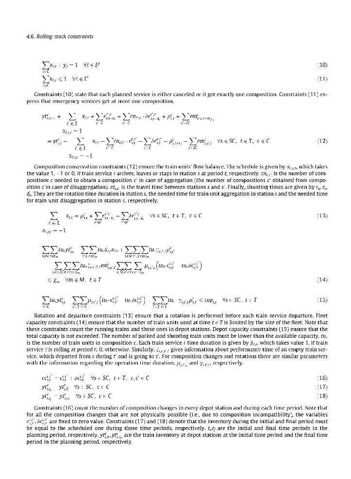
4.6. Rolling stock constraints

Yjctf+y^l W e L p (10) ceC

X X C ^ 1 WeLe (11) ceC

Constraints (10) state that each planned service is either canceled or it get exactly one composition. Constraints (11) ex­press that emergency services get at most one composition.

y^t-i + Y Xf-f+Yei,U + Yi^t • KU+Pit+Y ^i^-^ I £ L c 'e(- c 'e(- s'eSC

=ytit+ Y xi,c + Ycnv-<t' + YSei't +Pit+rs + Yemis',t ^&sc, t e r , c&c (12) £ (z £ c'^C C'^C S'IESC

al,s,t = — 1

Composition conservation constraints (12) ensure the train units' flow balance. The schedule is given by atSih which takes the value 1, - 1 or 0, if train service £ arrives, leaves or stays in station s at period t, respectively. cncc, is the number of com­positions c needed to obtain a composition c' in case of aggregation (the number of compositions c' obtained from compo­sition c in case of disaggregation). etss, is the travel time between stations s and s'. Finally, shunting times are given by rs, es, ds. They are the rotation time duration in station s, the needed time for train unit aggregation in station s and the needed time for train unit disaggregation in station s, respectively.

Y X?,c=Pit + Y<'t-es+Y<U VS€SC, t€T, C€C (13)

%l,s,t = — 1

YY^ytit+EE^ft,^ + YYY^ttPiv seSCceCm leL ceCm seSCeeTceCm

+ YYYtUc^.t'.temis',tYY Y ^.fA^^ + ^Kf, s.^'£SCeeTC£Cm seSCt'eTc,c'£Cm

^Xm VmcM, tcT (14)

Y tucyt{f + YY^,t;t(tuce£ + tuc5e% \ + \^Juc • ys^tplf, < capst VscSC, t€T (15) ceC f e T ceC feT ceC

Rotation and departure constraints (13) ensure that a rotation is performed before each train service departure. Fleet capacity constraints (14) ensure that the number of train units used at time t e T is limited by the size of the fleet. Note that these constraints count the running trains and those ones in depot stations. Depot capacity constraints (15) ensure that the total capacity is not exceeded. The number of parked and shunting train units must be lower than the available capacity. tuc

is the number of train units in composition c. Each train service £ time duration is given by ftt, which takes value 1, if train service £ is rolling at period t; 0, otherwise. Similarly, ^f,t gives information about performance time of an empty train ser­vice, which departed from s during f and is going to s'. For composition changes and rotations there are similar parameters with the information regarding the operation time duration, fist, t and yst,t, respectively.

cccsdt = eg' + 5e$ Vs €SC, r e T, c,d e C (16)

ytlti=yfsfi VscSC, ccC (17)

3 ^ = J * U VseSC, ceC (18)

Constraints (16) count the number of composition changes in every depot station and during each time period. Note that for all the composition changes that are not physically possible (i.e., due to composition incompatibility), the variables e g , <5eg are fixed to zero value. Constraints (17) and (18) denote that the inventory during the initial and final period must be equal to the scheduled one during those time periods, respectively. titt[ are the initial and final time periods in the planning period, respectively. ytc

s0,ytcsoo are the train inventory at depot stations at the initial time period and the final time

period in the planning period, respectively.

5. Computational experiments

Our experiments are based on realistic cases drawn from RENFE's regional network in Madrid for 2008 (Fig. 1). This net­work is composed of 10 different lines with almost 100 stations, carrying more than one million passengers every day. The network has double tracks on all segments.

We used for our tests a personal computer with an Intel Core 2 Quad CPU at 2.83 GHz and 8 GB of RAM, running under Windows 7 64-Bit, and we implemented the models in GAMS/Cplex 12.1.

The disrupted network. Our case study features a disruption where one of the two tracks between two stations is blocked: trains in different directions must share the remaining track. Also, some trains that were supposed to pass may turn back instead of entering the disrupted segment. The disruption starts at 8:00 a.m. and it lasts 120 min.

The disrupted segment is only used by trains belonging to the C5 line. The alternative paths for passengers of the C5 line include trips on the lines C3, C41, C42 and C5 (run by RENFE) as well as trips on the Metro network (run by another operator). Therefore we restrict the network to these lines only. The restricted network, depicted in Fig. 2, features 46 station, and about 12,000 trips in 760 timetable services. About 530,000 passengers use the restricted network, 47,000 of which are directly affected by the disruption.

The frequency on the C5 line is rather high: there is a train service every 3 min in the peak hours and every 10 min in the off-peak hours. Lines C3, C41 and C42 have a slightly lower frequency: trains in the peak hours run every 6 min and every 16 min in the off-peak hours. The considered lines are served with two train units types with a capacity of 588 and 757, respectively. Trains in the Metro system run every 3 min and we assume that they have unlimited capacity.

C2 SEGOVIA p

t"0 C-4

M m e n a r l Visjo|

ParfluedeOcio

Sin Martin-delaVegi

C-3a AnmJuaG

C-3* CUENCA

Fig. 1. RENFE's rapid transit network around Madrid.

Line C3: AR-ATO 56.5 Km Line C41: PA-VIAL-ATO-COL 58.2 Km Line C42: PA-VIAL-ATO-ALC 47.4 Km LineC5: HU-FU-VIAL-OR-ATO-MO 43.6 Km

Fig. 2. Network topology while the blockage is active.

The proposed model decides on the schedule both for the disruption period and for the forthcoming recovery plan. Trains can be canceled during the entire time horizon. As the cancellation costs are very high, they will only occur when they are unavoidable. However, there also exists the possibility of scheduling additional emergency services in order to maintain the offered capacity in the non-disrupted areas. All in all, the disrupted area is likely to see a reduced number of timetable ser­vices, and the passengers will take this into account in their path selection.

Passenger demand split. The disruption has no direct effect on the passengers of lines C3, C41 and C42; they will just stick to their intended path. Passengers of line C5, however, may have multiple traveling options: they can remain in the line C5 waiting for a direct or indirect train; they also can make use of lines C3, C41 and C42 as well as of the Metro network. Depending on their origin and destination, passengers of line C5 may choose any combination of these mentioned alterna­tives. For example, they may use line C5, then transfer to line C41, and finally come back again to line C5 for the last part of their journey.

In an undisturbed scenario the entire demand is covered by the passenger services. Once the disruption has started, we compute the new passenger demand with the multinomial logit model. Consequently, an anticipated schedule is needed. This anticipated schedule is obtained considering the following: the demand is asymmetric and the track capacity is reduced. The best schedule for passengers would be the one providing proportionate frequency values to the demand in each direc­tion. Then, once the track capacity and the demand to be attended (in an undistrubed scenario) are known, the anticipated timetable is provided to the multinomial logit model.

In our case study, the multinomial logit model gives the following output. In total, 26.2% of the demand in line C5 choose to stay in line C5; 44.3% will go through a combination of lines C5 and lines C3, C41 and C42; finally, 29.5% of the demand will go for a combination of line C5 and the Metro network.

5. J. Recovery solutions

In this section we solve the integrated optimization model for the presented disrupted network. The model's objective function is a combination of different terms, their relative importance can express different overall managerial goals. Below we consider the same disruption with several different objective weight settings, and we discuss the corresponding optimal solutions.

The optimization model can make timetabling decisions (cancellation of existing services or insertion of emergency ser­vices) as well as rolling stock decisions on the disrupted line C5. In addition, the model may change the rolling stock sched­ules of the undisrupted lines C3, C41 and C42 in order to adjust the train capacities to the elevated demand figures. We do forbid, though, the cancellation of any of the C3, C41 and C42 services.

Line C5 is independent from lines C3, C41 and C42, they do not share any rolling stock resources. Therefore the optimi­zation model decomposes into two independent subproblems: one for the disrupted line C5, and one for the undisrupted

lines C3, C41 and C42. Below we present the solutions of the two subproblems. The detailed solutions for each of the sub-problems are presented in the Appendix A.

We solve five different variants of the ITRSRM model. Table 1 summarizes our results by letting each column represent one of the five ITRSRM solutions. Each column contains six characteristics of the given solution. Rows TSOC and EMOC give the total operational costs for passenger train services and empty movements, respectively. Row DP gives the number of de­nied passengers. SC is the number schedule changes which is a measure to estimate how easy is it for the operator to imple­ment the recovery plan; SC accounts for rolling stock changes, empty movements changes and cancellations. Finally, row ST gives the solution time in seconds.

We want to emphasize that the optimization model considers arc-based demand figures. Therefore, the number of denied passengers will also be arc based. However, this is a heuristic approach since a denied passenger would still be counted by the model on the following arc. Row DP-est is the number of denied passengers as estimated by the optimization model, while row DP gives the exact number of denied passengers and is calculated in a post-processing step.

The solution P&O arises by minimizing the combination of passenger and operator costs (i.e., all the terms in the objective function).

The solution P&O-RS is obtained by minimizing the combination of passenger and operator costs subject to the additional constraint that all non-canceled services must keep their originally planned rolling stock composition. That is, the model can only cancel trains or add emergency services.

The solution P&O-RS-EM is similar to P&O-RS; the additional constraint is that non-canceled empty trains must be un­changed compared to the undisrupted schedule.

The solution Operator is obtained by minimizing the operator's costs only. Finally, the solution Pax is obtained by minimizing the number of denied passengers (DPs) as a sole objective. Rolling

stock related costs are not taken into account and we assume an unlimited fleet size. In fact, the solution uses more than 300 empty movements. The objective value of Pax is a reference lower bound for the passenger service quality of the other, more realistic, solutions.

We first notice that the lowest possible DP is very well approached whenever the passenger costs are part of the objective (solutions P&0} P&O-RS and P&O-RS-EM). The service quality deteriorates slightly as we impose more and more restriction on the schedules. Solution Operator, on the other hand, results in almost 15,000 denied passengers, eight times more than what is achieved in the other solutions. We will elaborate on the gap between DP and DP-est below in Section 5.2.

The operational costs (TSOC and EMOC) do not show much variation. As one may expect, Operator is the best, but P&O, P&O-RS and P&O-RS-EM) are reasonably close to it. Solution Pax cannot be compared to the other ones as it uses unlimited rolling stock and a huge number of empty movements.

The ease of the recovery process is measured by the number of schedule changes (SCs). The results are conform with our intuition: solutions P&O-RS-EM, P&O-RS and P&O have increasingly more freedom to change the schedules, and they indeed use this freedom to reach a better service quality. Based on preliminary discussions with practitioners, the SC values of 25-40 all have a good chance to be implementable in practice. Solution Operator needs an even higher SC in order to improve slightly on the operational costs. Solution Pax has little practical value.

The solution times (STs) range from a few seconds to a few minutes. Therefore the proposed model fits well in the time frame of real life disruption management.

5.2. Comparison of P&O and Operators

In this section we have a closer look at two radically different solutions: P&O and in Operator. We omit P&O-RS and P&O-RS-EM because their characteristics are very similar to those of P&O.

Figs. 3 and 4 depict the passenger demand as a function of time; Fig. 3 belongs to P&O, Fig. 4 belongs to Operator. Each chart contains two curves: the higher curve indicates the sum of all passenger demand figures at a given time, while the lower curve shows the denied passenger demand at that time.

The denied demand in solution P&O (Fig. 3) is indeed a very small fraction of the whole demand. This gives an empirical validation for our passenger modeling approach: in spite of the simple per-arc demand structure, the model treats the over­whelming majority of passengers accurately; in fact, the assigned capacity covers most of the passenger demand. This val­idation does not hold for the case of Operator (Fig. 4). By disregarding the altered passenger demand pattern, the model

Table 1 Recovery solutions.

Item P&O P&O-RS P&O-RS-EM Operator Pax

TSOC EMOC #DP #DP-est #SC ST

166338.06 6984.63 1839 5221 40 206

165880.1 7965.67 2254 5938 30 114

166778.! 6900.07 2692 7147 25 69

163677.74 5537.27 14974 53578 45 38

188241.2 219833.66 1576 4853 982 183

500 521 543605 626 6+S 710 732754816333 900 322344 1010 1040 1111 11421212 1243 1314 1344 1415 1446 1516 1547 161B 1B43 1713 17501320 1351 1522 1952 2023 2054 2124 2155 2226 2253 2327 2357 2423

Fig. 3. Passenger demand in the solution P&O: number of requested trips (higher curve) and number of denied trips (lower curve).

500521 543B05626643710732754B16B3S900922344 103 0 1040 1111 1142 1212 1243 1314 1344 1415 1446 1516 1547 1613 1643 1713 1750 1S20 1351 1922 1952 2023 2054 2124 2155 2226 2253 2327 2357 2423

Fig. 4. Passenger demand in the solution Operator, number of requested trips (higher curve) and number of denied trips (lower curve).

chooses insufficient train capacities and thereby heavily overestimates the number of denied passengers. Even the correct DP value is very high, denied passengers constitute a significant part of the total demand.

The inclusion of passenger costs guides the model towards a good timetable as illustrated by the following observation. The disrupted line segment allows for one train at a time to pass. Table 2 shows how many trains per direction are scheduled in the two considered solutions. The undisrupted solution is asymmetric, so is the demand: there are more trains from the suburbs towards the city center during the morning rush hour. Solution P&O maintains the same pattern, even though the number of passing trains is reduced. However, solution Operator behaves differently because the disruption appears to create a relative rolling stock shortage on the suburban side.

Finally, we analyze the price of the recovery plan P&O as compared with the original rolling stock assignment. The results are summarized in Table 3. We give more details about the solutions in Appendix A.

The recovery schedule has lower operating costs for train services which follows from the fact that some train services are canceled. On the other hand, the recovery schedule has higher empty movements costs because more empty movements are needed in order to match capacity requirements and rolling stock resources. By definition, the original schedule has no sche­dule changes. Finally, we notice that the recovery schedule needs a higher computational time, among others due to the additional complexity of the timetabling decisions.

5.3. Iterative use of the two-step approach

The results in Sections 5.1 and 5.2 arise from a single use of the two-step approach where the passenger demand is com­puted for an anticipated fictitious timetable. Recall that the passengers' path choice depends on the timetable but not on the rolling stock assignment. One may wonder how stable is this demand: does the optimized timetable lead to another travel path choice than what we anticipated?

In order to answer this question, we embed the basic two-step algorithm in an iterative framework. The first iteration is what we have done so far. In each subsequent iteration, we re-compute the passenger path choice based of the last iteration's timetable. The results in this section are limited to the objective of P&O.

It turns out in our computational experiments that the passenger demand barely changes after the first iteration. When compared to the first iteration's passenger path choice, as few as 619 passengers decide to choose a different path in the second iteration; this is very little compared to the 47,000 passengers of the C5 line during the disruption. The 619 passen­gers are roughly equal to the capacity of just one rolling stock unit. Spread over a 2-h time period and 23 departure stations, the 619 passengers may very well be less than the daily fluctuation of the passenger numbers.

Figs. 5-7 give some deeper insight of these numbers by showing the passenger demand spread in time (during the dis­ruption) for the first two iterations. Figs. 5 and 6 plot the demand for two particular alternative routes (namely: the combi­nation of lines C5 and C41/C42, and the combination of line C5 and the Metro network, respectively). Fig. 7 shows the demand that remains on line C5. Mind that the graphs have different vertical scales.

There are two curves in each of the graphs: The lighter gray curve represents the demand in the first iteration and the black one the demand in the second iteration. The vertical difference between the curves never exceeds the value of 300. As a consequence, the second iteration leads to a timetable and rolling stock schedule that is almost identical to the output of the first iteration. The changes of the second iteration's solution, as compared to the first's, are as follows:

• The two timetables run the same set of services; seven emergency services are shifted by 3 min, and one service is shifted by 7 min.

• There are no rolling stock changes. • The second iteration has 1718 denied passengers. That is, 121 additional passengers are able reach their destination

within the restricted network; these passengers were denied in the first iteration. • The total travel time for passengers during the disruption is similar in both iterations: in the first iteration it was

742561.5 min and in the second one it is 743972.5 min. However, the total travel time before the disruption was 623,910 min. Obviously, the total travel time is increased during the disruption. Regarding the average travel time per passenger we have that it was 13.27 min before the disruption, 16.18 min in the first iteration and 16.25 in the second iteration (this average travel time is obtained for passengers traveling from 8:00 a.m. to 10:00 a.m.).

The virtually immediate stabilization of the iterative approach is largely due to a successful initial estimation of the train frequencies on the disrupted segment. More complex disruptions and severe rolling stock limitations may result in timeta­bles that cannot match the initially estimated train frequencies. In such cases the iterative framework is likely to be essential in order to obtain a realistic passenger path choice.

Table 2 Frequency values in line C5 between VIAL and OR.

Direction Operator P&O Undisrupted

VIAL -> OR 20 22 35 OR -> VIAL 22 18 30

Table 3 Recovery and original planning.

Schedule

Recovery Original

TSOC

166338.06 167937.28

EMOC

6984.63 5355.87

#SC

40

#DP

5221(1839)

ST

206 122.5

It 1

•It 2

8:00:00 3:30:00 9:00:00 9:30:00 10:00:00

Fig. 5. Passenger demand in the first and second iterations for the combination of lines C5 and C41/C42.

7 0 0

600

500

400

300

It 1

•It 2

3:00:00 3:30:00 9:00:00 9:30:00 10:00:00

Fig. 6. Passenger demand in the first and second iterations for the combination of line C5 and the Metro network.

5.4. Summary of the computational results

The proposed algorithmic framework allows us to find solutions for rather different managerial goals in a matter of min­utes. The solution P&O turns out to provide a particularly good balance between the optimization criteria: the passengers' costs and the operator's costs are simultaneously brought near to their respective lowest possible values.

When the passenger costs are part of the objective function, the denied demand turns out to be a very small part of the whole demand. This gives an empirical validation for our passenger modeling approach in that the model treats the over­whelming majority of passengers accurately.

In order to better capture the dynamic nature of the passengers' path choice, we implement our basic two-step algorithm in an iterative setting. The iterative framework does not improve the solution quality significantly in our experiments. The first iteration appears to estimate the passenger behavior well enough. Consequently, there are barely changes in the sche­dule of the second iteration. We do believe, though, that more complex disruptions may benefit from multiple iteration.

3500

3000

2500

2000

1500

1000

500

It 1

' It 2

8:00:00 8:30:00 9:00:00 9:30:00 10:00:00

Fig. 7. Passenger demand in the first and second iterations for the line C5.

Table 4 Line C5 recovery solutions.

Item P&O P&O-RS P&O-RS-EM Operator Pax

TSOC EMOC #ES #CC #cr #DP #DP-est #RSC #EMC ST

78186.26 2775 36 24 25 1116 3138 6 4 164

78042.58 3874.84 30 20 24 1435 3535 0 6 85

78941.34 2809.24 36 22 25 1873 4744 0 0 40

76097.26 1788.32 10 18 17 13228 48465 14 4 16

87195.88 125095.14 43 68 28 881 2822 121 396 150

Table 5 Solutions for lines C3, C41 and C42.

Item P&O P&O-RS-EM Operator Pax

TSOC EMOC #CC #DP #DP-est #RSC #EMC ST

88151.8 4209.63 32 723 2083 2 3 42

87837.52 4090.83 34 819 2403 0 0 29

87580.48 3748.95 32 1746 5113 4 6 22

101045.32 94788.52 132 695 2031 132 305 33

Table 6 Line C5 recovery and original planning.

Schedule

Recovery Original

TSOC

78186.26 80099.76

EMOC

2775 1265.04

#CC

24 20

#CT

25

#DP

3138(1116)

ST

164 24.5

Table 7 Lines C3, C41 and C42 recovery and original planning.

Schedule TSOC EMOC #CC #CT #DP ST

Recovery Original

88151.8 87837.52

4209.63 4090.83

32 34

2083(723) 42 98

6. Conclusions

In this paper we study the recovery problem of rapid transit networks. When dealing with a disruption, the operator wants to offer a good service quality service while the system is being recovered to the original planning.

The main contribution with respect the literature is that the approach decides on the timetable and on the rolling stock schedule using an integrated optimization model accounting for the passenger demand behavior. In contrast, the majority of the related literature on railway resource rescheduling does not deal with changing demand patterns. Therefore this paper considers an integrated timetabling and rolling stock recovery model that also accounts for passengers. We propose a two-step approach to adjust the timetable and the rolling stock assignment, and we explicitly take the passengers' reaction to the disruption into account. Our approach first computes the anticipated passenger demand. Then the integrated timetabling and rolling stock scheduling problem as a Mixed Integer Linear Programming model. Further, we embed the two-step ap­proach in an iterative framework.

In computational tests on realistic instances of RENFE, our method is able to find solutions with a very good balance be­tween the managerial goals. Preliminary discussions with practitioners revealed that the solutions captured all important real-life restrictions, and have a good chance to be implementable in practice. Our computational times amount to a few minutes which is sufficiently close to the needs of real-time decision making. This is a great advantage with respect to the current system of manual re-planning where planners work under great time pressure.

In our future research we are going to embark on a deeper study of Pareto optimal solutions in order to give the operator a wider and deeper insight in the different recovery solutions depending on the objective function terms weights. Further re­search needs to refine the multinomial logit model in order to better capture the passengers' behavior. For this purpose more real-life data must be gathered and studied. Another quite challenging option would be to develop an optimization model to deal with the complex interaction of timetable, rolling stock and passengers.

Acknowledgments

This research was supported by Project Grants TRA2008-06782-C02-01 and TRA2011 -27791-C03-01 by the "Ministerio de Economia y Competitividad, Spain". We also want to thank Evelien van der Hurk (Rotterdam School of Management) and the anonymous referee for their helpful comments on the paper.

Appendix A. Detailed results

The following tables display the detailed results for each of the subproblems. Table 4 shows computational results for line C5 and Table 5 for lines C3, C41 and C42.

We add some new information: the number of emergency services (#ES) and the number of composition changes (#CC). SC are disaggregated into the number of canceled trains (#CT), the number of Rolling Stock Changes (#RSC) and the number of Empty Movements Changes (#EMC).

Lacking the option to cancel trains in lines C3, C41 and C42 the solution for column P&O-RS-EM gives rise to the very same schedule as the one operated under normal (undisrupted) conditions. For this solution, there are substantially more denied passengers than in Pax or even in P&O. This is because the offered capacity in a normal scenario is not enough to accommo­date the additional demand.

Tables 6 and 7 compare the recovery and original planning for lines C5 and C3, C41 and C42, respectively.

References

Ben-Akiva, M., Lerman, S.R., 1985. Discrete Choice Analysis: Theory and Application to Travel Demand. The MIT Press, Cambridge, Massachusetts. Bratu, S., Barnhart, C, 2006. Flight operations recovery: new approaches considering passenger recovery. Journal of Scheduling 9 (3), 279-298. Budai, G., Maroti, G., Dekker, R., Huisman, D., Kroon, LG., 2010. Rescheduling in passenger railways: the rolling stock rebalancing problem. Journal of

Scheduling 13, 281-297. Cacchiani, V., Caprara, A., Galli, L, Kroon, LG., Maroti, G., Toth, P., 2012. Railway rolling stock planning: robustness against large disruptions. Transportation

Science 46, 217-232. Cadarso, L, Marin, A., 2011. Robust rolling stock in rapid transit networks. Computers & Operations Research 38 (8), 1131-1142. Cadarso, L, Marin, A., 2012. Integration of timetable planning and rolling stock in rapid transit networks. Annals of Operations Research 199 (1), 113-135. Clausen, J., 2007. Disruption Management in Passenger Transportation - from Air to Tracks. In: Proceedings at ATMOS 2007 - 7th Workshop on Algorithmic

Methods and Models for Optimization of Railways, ISBN: 978-3-939897-04-0. de Almeida, D., Trouve, F., Hebben, B., 2003. A Decision Aid Module for Resources Rescheduling when Managing Disturbances. Technical Report, Presented at

the World Congress on Railway Research. Dumas, J., Soumis, F., 2008. Passenger flow model for airline networks. Transportation Science 42 (2), 197-207. Dumas, J., Aithnard, F., Soumis, F., 2009. Improving the objective function of the fleet assignment problem. Transportation Research Part B: Methodological

43 (4), 466-475. Filar, J., Manyem, P., White, K., 2000. How airlines and airports recover from schedule perturbations: a survey. Annals of Operations Research 108,315-333. Jarrah, A.I.Z., Yu, G., Krishnamurthy, N., Rakshit, A., 1993. A decision support framework for airline flight cancellations and delays. Transportation Science 27

(3), 266-280. Jespersen-Groth, J., Potthoff, D., Clausen, J., Huisman, D., Kroon, LG., Maroti, G., Nielsen, M., 2009. Disruption management in passenger railway

transportation. In: Ahuja, R, Mohring, R, Zaroliagis, C, (Eds.), Robust and Online Large-Scale Optimization, Lecture Notes in Computer Science, vol. 5868, pp. 399-421.

Kroon, L.G., Huisman, D., 2011. Algorithmic support for railway disruption management. In: Nunen, Jo A.E.E., Huijbregts, P., Rietveld, P. (Eds.), Transitions Towards Sustainable Mobility. Springer, Berlin Heidelberg.

Nielsen, L.K., 2011. Rolling Stock Rescheduling in Passenger Railways. PhD. Thesis. Erasmus Research Institute of Management, Rotterdam School of Management (RSM). ISBN 978-90-5892-267-0.

Nielsen, LK., Kroon, L.G., Maroti, G., 2012. A Rolling Horizon Approach for Disruption Management of Railway Rolling Stock. European Journal of Operational Research 220 (2), 496-509.

Ortuzar, J.D., 2001. On the development of the of nested logit model. Transportation Research Part B 35, 213-216. Rosenberger, J.M., Johnson, E.L., Nemhauser, G.L., 2003. Rerouting aircraft for airline recovery. Transportation Science 37, 408-421. Stojkovic, G., Soumis, F., Desrosiers, J., Solomon, M., 2002. An optimization model for a real-time flight scheduling problem. Transportation Research Part A

36, 779-788. Thengvall, B., Yu, G., Bard, J., 1998. Balancing user preferences for aircraft schedule recovery during irregular operations. HE Transactions 32,181-193. Walker, C.G., Snowdon, J.N., Ryan, D.N., 2005. Simultaneous disruption recovery of a train timetable and crew roster in real time. Computers & Operations

Research 32, 2077-2094.