RECOVER SOUTHERN ESTUARIES PERFORMANCE MEASURES: IDENTIFICATION OF HYDROLOGY -

SALINITY RELATIONSHIPS FOR COASTAL ESTUARIES AND ANALYSIS OF INTERIM CERP

UPDATE SCENARIOS

Contract No. DACW17-02-D-0009

FINAL PROJECT REPORT

Principal Investigator: Frank E. Marshall III, PhD, P.E.

September, 2005

ENVIRONMENTAL CONSULTING AND TECHNOLOGY, INC. 340 NORTH CAUSEWAY

NEW SMYRNA BEACH, FLORIDA 32169 (386) 427-0694

TABLE OF CONTENTS Section Page I. BACKGROUND 1 A. General 1 B. Hydrology and Other Factors Affecting Salinity 2 C. Data for Model Development and Simulations 6

D. Model Development 10

II. FLORIDA BAY ANALYSIS 14 A. General 14

B. Study Area and Data 14 C. Florida Bay Models 15 D. Model Error Statistics 26 E. Florida Bay Analysis Discussion 30

III. BARNES SOUND AND MANATEE BAY ANALYSIS 33 A. Study Area and Data 33 B. Model Development 34

C. Manatee Bay and Barnes Sound Discussion 37 IV. ICU RUNS AND PERFORMANCE MEASURES 39 A. General 39 B. Simulation Procedure 39 C. ICU Salinity Simulations 43 D. Comparison of ICU Runs 43 E. ICU Runs Discussion 55 V. POST-PROCESSING ACTIVITIES 58 VI. REFERENCES 59

i

LIST OF TABLES Table Page

1 Summary of Information about the monitoring Stations and Salinity

Data 7

2 Summary of Information about the Independent Variables used in model development and verification for Florida Bay MLR Salinity Models

8

3 Comparison of Model Uncertainty Statistics for SES MLR Salinity Models, Developed for this Project

29

4 Comparison of Model Uncertainty Statistics for IOP/CES1 MLR Salinity Models, Developed Previously

29

5 Comparison of Model Uncertainty Statistics for MLR Salinity Models

37

6 Adjustments that were made to the output of the 2 x 2 Model for use in the MLR Salinity models for the ICU Simulations

44

LIST OF FIGURES

Figure Page

1 Study Area 4 2 Monitoring Station Map 5 3 A comparison of the variability in observed data for Craighead

Pond (CP) water level, P33 water level, and Key West sea surface level for the example period March 1971 through March 1983 (M = March)

11

4 Plot of u wind vector for the year 2000 as measured at Miami and Key West

12

5 Plot of v wind vector for the year 2000 as measured at Miami and Key West

12

6 Comparison of Observed and Simulated Daily Data for the Joe Bay MLR Model. Calibration is March 24, 1995 – October 31, 2002; Verification is March 24, 1994 – March 23, 1995

17

7 Comparison of Observed and Simulated Data for the Little Maderia Bay Extended Period MLR Model. Calibration is August 25, 1988 – October 31, 2001; Verification is November 1, 2001 – October 31, 2002

17

8 Comparison of Observed and Simulated Daily Data for the Terrapin Bay MLR Model. Calibration is March 24, 1995 – October 31, 2002; Verification is March 24, 1994 – March 3, 1995

18

9 Comparison of Observed and Simulated Daily Data for the Long Sound MLR Model. Calibration is March 24, 1995 – October 31, 2002; Verification is March 24, 1994 – March 3, 1995

18

10 Comparison of Observed and Simulated Daily Data for the Whipray Basin MLR Model. Calibration is March 24, 1995 – October 31, 2002; Verification is March 24, 1994 – March 3, 1995

19

ii

LIST OF FIGURES (Continued)

Figure Page

11 Comparison of Observed and Simulated Daily Data for the Duck

Key MLR Model. Calibration is March 24, 1995 – October 31, 2002; Verification is March 24, 1994 – March 3, 1995

19

12 Comparison of Observed and Simulated Daily Data for the Butternut Key MLR Model. Calibration is March 24, 1995 – October 31, 2002; Verification is March 24, 1994 – March 3, 1995

20

13 Comparison of Observed and Simulated Data for the Taylor River MLR Model. Calibration is March 24, 1995 – October 31, 2002; Verification is March 24, 1994 – March 3, 1995

20

14 Comparison of Observed and Simulated Data for the Highway Creek MLR Model. Calibration is March 24, 1995 – October 31, 2002; Verification is March 24, 1994 – March 3, 1995

21

15 Comparison of Observed and Simulated Data for the Little Blackwater Sound MLR Model. Calibration is March 24, 1995 – October 31, 2002; Verification is March 24, 1994 – March 3, 1995

21

16 Comparison of Observed and Simulated Data for the Bob Allen Key MLR Model. Calibration is September 9, 1998 – October 31, 2002; Verification is September 9, 1997 – September 8, 1998

22

17 Comparison of Observed and Simulated Daily Data for the Garfield Bight MLR Model. Calibration is March 6, 1997 – December 31, 2002; Verification is March 6, 1996 – March 5, 1997

22

18 Comparison of Observed and Simulated Daily Data for the Clearwater Pass MLR Model. Calibration is May 10, 1997 – December 31, 2002; Verification is May 10, 1996 – May 9, 1997

23

19 Comparison of Observed and Simulated Daily Data for the Whitewater Bay MLR Model. Calibration is August 27, 1996 – December 31, 2002; Verification is August 27, 1995 – August 26, 1996

23

20 Comparison of Observed and Simulated Daily Data for the North River MLR Model. Calibration is March 6, 1997 – December 31, 2002; Verification is March 6, 1996 – March 5, 1997

24

21 Comparison of Observed and Simulated Daily Data for the Gunboat Island MLR Model. Calibration is March 22, 1997 – December 31, 2002; Verification is March 22, 1996 – March 21, 1997

24

22 Comparison of Observed and Simulated Daily Data for the Shark River MLR Model. Calibration is January 1, 1997 – December 31, 2002; Verification is January 1, 1996 – December 31, 1996

25

23 Comparison of Observed and Simulated Daily Data for the Middle Key MLR Model. Calibration is March 24, 1995 – October 31, 2001; Verification is March 24, 1994 – March 3, 1995

36

iii

iv

LIST OF FIGURES (Continued)

Figure Page

24 Comparison of Observed and Simulated Daily Data for the

Manatee Bay MLR Model. Calibration is March 24, 1995 – December 31, 2000; Verification is March 24, 1994 – March 3, 1995

36

25 Comparison Between 2 x 2 Model Output and Observed Data for Stage Station P33

41

26 Comparison Between 2 x 2 Model Output and Observed Data for Stage Station EVER7

41

27 Comparison Between 2 x 2 Model Output and Observed Data for Stage Station CP

42

28 Comparison Between 2 x 2 Model Output and Observed Data for Stage Station SWEVER1

42

29 Joe Bay-Annual Mean, Monthly Mean, and 25th/75th Quartile 45 30 Little Maderia Bay-Annual Mean, Monthly Mean, and 25th/75th

Quartile 45

31 Terrapin Bay-Annual Mean, Monthly Mean, and 25th/75th Quartile 46 32 Garfield Bight-Annual Mean, Monthly Mean, and 25th/75th Quartile 46 33 Long Sound-Annual Mean, Monthly Mean, and 25th/75th Quartile 47 34 Little Blackwater Sound-Annual Mean, Monthly Mean, and 25th/75th

Quartile 47

35 Highway Creek-Annual Mean, Monthly Mean, and 25th/75th Quartile 48 36 Taylor River-Annual Mean, Monthly Mean, and 25th/75th Quartile 48 37 Clearwater Pass-Annual Mean, Monthly Mean, and 25th/75th

Quartile 49

38 Whitewater Bay-Annual Mean, Monthly Mean, and 25th/75th Quartile

49

39 North River-Annual Mean, Monthly Mean, and 25th/75th Quartile 50 40 Gunboat Island-Annual Mean, Monthly Mean, and 25th/75th Quartile 50 41 Shark River-Annual Mean, Monthly Mean, and 25th/75th Quartile 51 42 Whipray Basin-Annual Mean, Monthly Mean, and 25th/75th Quartile 51 43 Duck Key-Annual Mean, Monthly Mean, and 25th/75th Quartile 52 44 Butternut Key-Annual Mean, Monthly Mean, and 25th/75th Quartile 52 45 Bob Allen Key-Annual Mean, Monthly Mean, and 25th/75th Quartile 53 46 Manatee Bay-Annual Mean, Monthly Mean, and 25th/75th Quartile 53 47 Middle Key-Annual Mean, Monthly Mean, and 25th/75th Quartile 53 48 Difference in Water Surface Elevation at Craighead Pond (CP) for

NSM 4.6.2, and CERP2000 and CERP0 Produced by MLR Salinity Models

57

RECOVER SOUTHERN ESTUARIES PERFORMANCE MEASURES:

IDENTIFICATION OF HYDROLOGY - SALINITY RELATIONSHIPS FOR COASTAL ESTUARIES AND ANALYSIS OF INITIAL CERP UPDATE

SCENARIOS

Contract No. DACW17-02-D-0009

FINAL PROJECT REPORT

I. BACKGROUND

A. General Environmental Consulting & Technology, Inc. (ECT) working as a sub-consultant to Tetra Tech Inc., has been contracted to support the U.S. Department of the Army, Corps of Engineers, Jacksonville District RECOVER branch with the identification of hydrology - salinity relationships needed to create Performance Measures (PMs). These PMs are to be used to evaluate water delivery alternatives for the Comprehensive Everglades Restoration Plan (CERP) by employing hydrologic model output from the South Florida Water Management Model (SFWMM or 2X2 Model) to predict salinities downstream in coastal estuaries. Translating the water level measured by gauges and other hydrologic structures into salinities in coastal basins requires an analysis of statistical relationships between historical hydrology and resulting salinities in the subject south Florida water bodies. Other factors may also be important in quantifying these relationships, such as rainfall, wind and sea level. Once it is determined which gauges and structures are statistically significant for each basin, multivariate linear regression (MLR) models are to be developed for basins in Florida Bay, Barnes Sound / Manatee Bay, and the Shark Slough discharge area north of Cape Sable. These new models are to be combined with the existing MLR models prepared previously for Everglades National Park (ENP) by Cetacean Logic Foundation, Inc. to create a suite of models that describes the temporal and spatial variation in the south Florida area that receives drainage from the Everglades. The Regional Evaluation Team (RET) of RECOVER can then use the suite of models to simulate the salinity of coastal basins from SFWMM model output for various CERP project alternatives, thereby generating a key piece of information (salinity regime) on the effect of projects on the ecology of the embayments and open-water basins of Florida Bay. The Southern Estuaries Sub-team (Sub-team) of RET has been assigned with the responsibility of developing salinity performance measures that utilize the statistical models to evaluate alternatives for the Interim CERP Update. The Sub-team recommended the work described in this report.

1

The work described in this report builds on the previous salinity model work that has been done in some of the coastal basins of Florida Bay by ENP. As research sponsored by the Critical Ecosystem Studies Initiative (CESI), multivariate linear regression (MLR) models were investigated for use in simulating salinity (Marshall, 2003a; Marshall, 2004) and were found to be capable of providing reasonable daily estimates of salinity in the near shore embayments that were investigated. The techniques were successfully applied for the first time in the evaluation of alternative water delivery schemes as part of the Interim Operations Plan (IOP) Congressional report activities (Marshall, 2003b, 2005). For this project, four tasks were completed, each resulting in the preparation of a draft task report that was distributed electronically. These task reports were incorporated into this single-volume project report. The four tasks that were completed were:

(1) the Florida Bay analysis, (2) the Barnes Sound and Manatee Bay analysis, (3) the ICU alternative simulations, and (4) the post-processing activities.

Significant additional information was added to the task reports to complete the compilation of the four task reports into this Project Report.

B. Hydrology and Other Factors Affecting Salinity Freshwater flowing into ENP across Tamiami Trail moves south and southwest towards Florida Bay and the southwest Gulf of Mexico coast, as shown on the study area map, Figure 1 and the more detailed Figure 2. Most of the freshwater flows through Shark River Slough into the Gulf, but some freshwater passes through Taylor Slough, and is distributed into northeast Florida Bay and Barnes Sound / Manatee Bay / Card Sound, augmented by flows from the C-111 Canal system and seepage from stored surficial aquifer groundwater beneath the topographic high of the Atlantic Coastal Ridge on which metropolitan Miami is built. The contribution of groundwater and the effect on salinity variation in Florida Bay and Biscayne Bay is not fully understood. Rainfall in south Florida typically exhibits distinctive wet and dry season patterns but is variable spatially. The wet season pattern is driven by tropical weather and sea breeze interactions, with frequent storms that exhibit wide spatial distributions. Rainfall data between gauges that are only tens of miles apart often show widely varying rainfall volumes for a single period of time during the wet season (May or June through October or November). In the dry season (November or December through April or May), rain is usually delivered by frontal systems, with wider spatial distribution of single events, and less frequent events compared to the wet season. Evaporation is also seasonal, but with a slightly different pattern than rainfall. This

2

difference in timing has a significant effect on the timing and quantity of fresh water delivered and therefore the salinity. Wind also has a seasonal pattern similar to rainfall. During the wet season the wind direction is predominately from the south and southeast, and during the dry season northerly wind is most common. Additionally, the sea surface elevation and the elevation of the water surface in Florida Bay have their own “seasonal” behavior, with the highest average water surface elevations in the Fall and a secondary high in the Spring. When a hurricane or other significant weather event occurs, wind and storm surge effects can alter the sea surface elevation dramatically over short periods. According to coastal aquifer theories, the salinity in the interface zone between strictly fresh (0-5 psu) and marine waters (33-35 psu) in Florida Bay is influenced by the freshwater head in the upland watershed (measured as the elevation of water in wells in the Everglades) competing with the elevation of water in Florida Bay and the Atlantic Ocean (Pandit, et al; 1991). The result, when combined with the physical features of the embayments, basins, and bays of Florida Bay (including the shallow banks) and wind effects is a complex situation for salinity variability. To-date, only statistical models have been capable of successfully simulating this variability on a daily basis.

3

4

5

C. Data for Model Development and Simulations

In choosing the data that are to be included in the analysis and ultimately the MLR salinity models, the end use of the models has to be considered. The SFWMM or 2X2 model has produced estimates of stage (water level) and flow of freshwater through the Everglades for a number of CERP scenarios. Daily values are available for 31- and 36-year overlapping periods. The 36-year (1965-2000) runs are of interest for this study. The effects of the specified water deliveries on the water levels in the Everglades are expressed in the output of each of the CERP 2X2 runs. The MLR salinity models were developed to use the 2X2 model output in conjunction with available long-term data for wind and sea surface water level to produce estimates of daily salinity for the 36-year period in Florida Bay, the southwest Gulf coast, and Barnes Sound and Manatee Bay. The simulated salinity time series can be analyzed for potential ecological impacts, either positive or negative, of the particular water management alternative. The independent variable data must be available for most, if not all of the 36-year period in order to populate the models and obtain estimates of salinity to be of use for the ICU evaluations. This requirement eliminates the direct use of evaporation for models or simulations since there are no observed daily data for the 36-year period, nor are there any evaporation models that are capable of producing reliable daily estimates. Flows through control structures are not as useful statistically for model development and simulation purposes compared to stages (water levels) in the Everglades. Although rainfall is an important hydrologic parameter for seasonal salinity variation, rainfall at monitoring stations in the Everglades are not highly correlated with salinity at the daily level. Instead, the stochastic effect of rainfall falling on the Everglades and the upstream watershed is integrated by the coastal aquifer system and expressed adequately in stage data. Wind speed and direction and sea level are highly correlated with salinity at the daily level, and are available for the 36-year period. For the above reasons, the data that were used to develop the MLR salinity models and generate the simulations include the following:

1. Stage (water level) in monitor wells in the Everglades, 2. Wind speed and direction measured at Miami and Key West, and 3. Sea surface elevation measured at Key West.

For model development, observed stage data are used. For simulations, the 2X2 Model output data are used for stage after adjustments are made. Model development and simulations use the same data bases for wind and sea level although the period of the simulation is longer.

6

Continuous salinity data extend back to 1988 at several locations in northeast Florida Bay. However, some of the stations have only been operational since 1996. For the previously developed CESI / IOP models the period of data used for model development begins on March 24, 1994. For the new models in this study, the longest period of data available was used. The period of record for all stations extends through October 31, 2002. Most series contained some missing values. No attempts were made to fill in data gaps or to eliminate outliers in either independent or dependent variable data sets, as the number of daily values for the shortest time series for the observed data exceeded 2000 values. The models were developed from observed data that have been collected at 15 to 60 minute increments and averaged to daily values. Salinity data are taken from the ENP Marine Monitoring Network (MMN) data base, Table 1. Details about these data can be found in Everglades National Park (1997a and 1997b), and Smith (1997, 1998, 1999, and 2001). A map showing the ENP MMN stations and the locations of the water level monitoring stations used for this study is presented as Figure 2. Wind data were obtained directly from the National Weather Service (Southeast Regional Climate Center) for Key West and Miami stations, and sea surface level data collected at Key West were obtained from the National Ocean Service website (Table 2). Wind data from Key West and Miami were used as these locations had the longest continuous records for wind and were considered to be representative of the regional wind patterns. Sea surface elevation data from Key West were considered to be representative of the average effect of oceanic water level influences, and, to some extent, the average water level patterns within Florida Bay. The stage data are ENP Physical Monitoring Network Everglades water levels. A limited number of continuous water level (stage) monitoring stations in the Everglades began recording data in the 1950’s (see Table 2), but most stage records date from the 1990’s.

7

Table 1. Summary of information about the monitoring stations and salinity data used in model development and verification for Florida Bay MLR salinity models. All salinity data were collected by ENP.

Station Name MMN

ID Variable Name

Developed For Location

Beginning 0f Record

Little Madeira Bay

LM ltmad CESI Near-shore, Central Florida Bay

4/28/1988

Terrapin Bay TB terbay CESI Near-shore, Central Florida Bay

9/12/1991

Long Sound LS longsound CESI Near-shore, Northeast Florida Bay

3/28/1988

Joe Bay JB joebay CESI Near-shore, Northeast Florida Bay

4/26/1988

Little Blackwater

Sound

LB ltblackwater CESI Near-shore, Northeast Florida Bay

9/11/1991

Garfield Bight GB garfield CESI, SES Near-shore, Central Florida Bay

7/3/1991

Taylor River TR taylorriver CESI Taylor Slough Mangrove Zone

5/12/1988

Highway Creek HC hiwaycreek CESI Panhandle Mangrove Zone

4/27/1988

Whipray Basin WB whipray CESI Open-water, Central Florida Bay

4/28/1988

Duck Key DK duck CESI Open-water, Eastern Florida Bay

4/26/1988

Butternut Key BN butternut CESI Open-water, Eastern Florida Bay

4/27/1988

Bob Allen Key BA boballen CESI Open-water, Central Florida Bay

4/27/1988

Clearwater Pass

CW clearwater SES Whitewater Bay 5/10/1996

Whitewater Bay East

WW whitewater SES Whitewater Bay 8/27/1995

North River NR norriv CESI, SES Southwest Coast 02/30/90

Gunboat Island GI gunboat SES Southwest Coast 3/22/1996

Shark River SR sharkriver SES Southwest 5/2/1996

Note: CESI = Critical Ecosystems Studies Initiative, SES = Southern Estuaries Sub-team

8

Table 2. Summary of information about the independent variables used in model development and verification for Florida Bay MLR salinity models. Variable Name Variable Type Units Data Source Location Beginning Date of Data

Record CP Water Level Ft, NGVD 29 ENP Craighead Pond 10/01/78

E146 Water Level Ft, NGVD 29 ENP Taylor Slough 03/24/94 EVER4 Water Level Ft, NGVD 29 ENP So. Of FL City 09/20/85 EVER6 Water Level Ft, NGVD 29 ENP So. Of FL City 12/24/91 EVER7 Water Level Ft, NGVD 29 ENP So. Of FL City 12/24/91 G3273 Water Level Ft, NGVD 29 ENP East of S.R. Slough 03/14/84 NP206 Water Level Ft, NGVD 29 ENP East of S.R. Slough 10/01/74 NP46 Water Level Ft, NGVD 29 ENP Rocky Glades 01/15/66 NP62 Water Level Ft, NGVD 29 ENP East of S.R. Slough 01/04/64 P33 Water Level Ft, NGVD 29 ENP Shark River Slough 02/15/53 P35 Water Level Ft, NGVD 29 ENP Shark River Slough 02/15/63 P37 Water Level Ft, NGVD 29 ENP Taylor Slough 01/15/53 P38 Water Level Ft, NGVD 29 ENP Shark River Slough 01/10/52

R127 Water Level Ft, NGVD 29 ENP Taylor Slough 04/11/84 SWEVER1 Water Level Ft, NGVD 29 SFWMD Panhandle 07/15/87

G1183 Water Level Ft, NGVD 29 USGS Homestead 01/05/61 S196A Water Level Ft, NGVD 29 USGS Homestead 08/08/84 G580 Water Level Ft, NGVD 29 USGS Miami 07/15/49

G3356 Water Level Ft, NGVD 29 USGS Florida City 10/23/85 UWNDKW E-W Wind N/A NWS Key West 01/07/57 VWNDKW N-S Wind N/A NWS Key West 01/07/57 UWNDMIA E-W Wind N/A NWS Miami 01/07/57 VWNDMIA N-S Wind N/A NWS Miami 01/07/57

KWWATLEV Sea Surface Elevation

MSL Key West NOS Key West 01/19/13

9

D. Model Development

The framework for the relationship between estuarine and coastal shelf salinity is a coastal aquifer system physical model with a dynamic balance between fresh and salt water bodies and a salinity transition zone from upstream freshwater (salinity = 0) to sea water (salinity = 35 psu; Pandit et al, 1991). In most of the coastal aquifer examples in the literature, the focus is the water table aquifer, with the primary concern being the location of the transition zone as a water supply issue of saltwater intrusion. For salinity modeling in an estuary the focus is the salinity in the interface transition zone. The well-known Ghyben-Herzberg principle describes the location of this interface as function of the height of the freshwater surface in the watershed relative to the height of the sea surface above a common datum, and the relative density of the water masses. When the sea surface level is high enough relative to the freshwater level (such as a normal dry season), the higher density salt water moves the interface landward, increasing the salinity at a fixed station in the transition zone. When the freshwater level is high enough relative to the elevation of the sea surface to overcome the increased density of the seawater (such as a typical wet season in the Everglades), the salinity will decrease at a fixed station in the transition zone. In a shallow estuary like Florida Bay the wind can cause the interface to translocate and also to mix. Therefore, it is reasonable to expect that there would be a correlation between salinity levels and these three factors, which is confirmed by a correlation matrix of the observed data (not presented) at the 95% level of significance, sometimes for lagged values on the order of days. However, each of these forcing factors (fresh water elevation, wind, sea surface elevation) has a different pattern of variability over time. Figure 3 presents a plot of water levels at Craighead Pond (CP) and at P33, and sea surface elevation at Key West for the period March 1971-March 1983. Though the values of CP and P33 cannot be compared directly with the values of Key West sea surface elevation, the variability patterns in each time series can be evaluated. It can be seen that the variability in the sea surface elevation (Kwwatlev) is more uniform from year-to-year than the year-to-year variability in CP and P33, reflecting the regularity of the harmonic components of the sea surface elevation. While the values of CP and P33 are, in general, lower in the dry season (November – May) and higher in the wet season (June – October), it can be seen that the variability in the minimum value reached for a dry period is greater than the variability in the maximum value reached, reflecting the importance of wet season rainfall, or rather the paucity of it. For example, in Figure 3 the minimum water level reached at CP for 1974 and 1975 is much lower than the values reached for 1976 and 1977. A similar situation can be seen for P33 for 1974 compared to the following years. However, for 1975, CP behaves similar to 1974 (both expressing drought conditions), while at P33 the water level is relatively high in the dry season in 1975.

10

Figure 3. A comparison of the variability in observed data for Craighead Pond (CP) water level, P33 water level, and Key West sea surface level for the example period March 1971 through March 1983 (M = March).

-2-1012345678

M-71

M-72

M-73

M-74

M-75

M-76

M-77

M-78

M-79

M-80

M-81

M-82

M-83

ft, N

GVD

, ft M

SL (k

ww

atle

v)

kwwatlev CP P33

In addition to the variability of watershed and sea / estuary water levels is the variability in wind speed and direction, used in the salinity models as vector quantities. Figure 4 presents the daily time series for 2000 for the u-component of the wind vector, and Figure 5 presents the same information for the v-component. Although vector data are sometimes difficult to interpret, it can be seen that the patterns of daily variability are very similar at the two stations for the v-component. For the u-component, the positive and negative values for the Key West data are larger, and the variability pattern during the wet season (May – September) is different than the rest of the year.

11

Figure 4. Plot of u wind vector for the year 2000 as measured at Miami and Key West.

-15-10-505

101520

D-99

J-00

F-00

M-00

A-00

M-00

J-00

J-00

A-00

S-00

O-00

N-00

D-00

uwndkw uwndmia

Figure 5. Plot of v wind vector for the year 2000 as measured at Miami and Key West.

-15-10-505

101520

D-99

J-00

F-00

M-00

A-00

M-00

J-00

J-00

A-00

S-00

O-00

N-00

D-00

vwndkw vwndmia

12

A step-wise multivariate linear regression process was used to determine the most appropriate linear combination of independent variables for each salinity model. In addition to the independent variables in Table 2, the list of potential variables for model inclusion also included several hydraulic gradient variables computed using the stage variables in Table 2. To begin the model development procedure, all independent variables were subjected to a cross-correlation analysis with daily salinity using SARIMA techniques to determine which of the variables were correlated with salinity, to check for lagged relationships, and to evaluate the level of correlation. Lags up to 50 days were initially reviewed, though it was found that lagged correlations never exceeded six days. Then the observed data of the significant correlated variables (current and lagged values) were input to a SAS© PROC REG routine that uses a step-wise regression process to identify the most statistically significant parameters for a multivariate linear regression equation. To ensure that only the most highly significant parameters were selected by this process, the significance level for parameter inclusion in the model was set at 99.9%, a very high level. Parameter inclusion in a model was also manually controlled by eliminating any seemingly correlated variables that acted contrary to known physical relationships (such as an increasing stage in the Everglades indicating an increase in salinity) which can occur when there are cross-correlation effects. These parameters were eliminated, and the step-wise process re-run iteratively. For some of the open-water salinity monitoring stations that are away from the direct influence of the freshwater in the watershed it was found that salinity models were improved when Everglades stage was replaced by the salinity at the near shore stations of Little Madeira Bay and Terrapin Bay. The following CESI / IOP salinity models were developed from Little Madeira Bay and Terrapin Bay salinity, wind vectors, and Key West sea surface elevation instead of the stage elevation in the Everglades:

1. Whipray Basin, 2. Butternut Key, 3. Duck Key, and 4. Bob Allen Key.

During model verification it was determined that the salinity estimates produced by these models were more closely simulating the observed values compared to models prepared using watershed water levels. The details on model development can be found in Marshall (2003b, 2004, and 2005). However, it means that simulation is a two-step process with the simulation of salinity at Little Madeira Bay and Terrapin Bay required before salinity at the open-water stations can be simulated.

13

II. Florida Bay Analysis

A. General

For the Florida Bay analysis the existing CESI / IOP statistical salinity models were combined with newly-developed models to create a suite of models that will be used for the ICU runs. MLR salinity models were previously prepared for the following ENP MMN Stations in Florida Bay and on the southwest Gulf coast:

i. Joe Bay ii. Little Madeira Bay iii. Terrapin Bay iv. Garfield Bight v. North River vi. Whipray Basin vii. Duck Key viii. Butternut Key ix. Taylor River x. Highway Creek xi. Little Blackwater xii. Bob Allen Key xiii. Long Sound.

For this project a replacement model for North River was prepared to provide a greater focus on Shark Slough water level stations, and the Garfield Bight model was improved. Additionally, new models were developed for the following ENP MMN stations:

i. Clearwater Pass ii. Whitewater Bay iii. Gunboat Island iv. Shark River.

B. Study Area and Data

The study area for the Florida Bay analysis encompasses northeastern, north, and central Florida Bay; the extreme southwestern coast of Florida in the Ten Thousand Islands to Cape Sable vicinity; and the Everglades watershed. All areas are within Everglades National Park (ENP). Freshwater comes across Tamiami Trail into Shark Slough from the north through the S-12 structures, and also is pumped directly into the upper reach of the C-111 Canal. Water in the C-111 Canal can be routed by a number of canals to Biscayne Bay, into the mangrove zone south of the S-18C structure through the degraded berm then into northeast Florida Bay, or into Manatee Bay when the S-197 structure is open. Most of the water in Shark Slough discharges into the Gulf of Mexico north of Cape Sable.

14

Some Shark Slough water passes into Taylor Slough and discharges into several of the upper embayments of Florida Bay. Groundwater stored in the Atlantic Coastal Ridge can also discharge into Taylor Slough, as well as into the mangrove zone area that can discharge eventually into Long Sound, Manatee Bay, or Barnes Sound. Alterations to freshwater flow patterns have occurred as a result of the construction of the water management system, including changes to quantity, timing, and spatial distribution.

C. Florida Bay Models For the previous CESI / IOP project, the following daily MLR salinity models had already been developed and were adopted for this project, as follows: JOE BAY = 37.1 - 3.1CP - 3.5 EVER6[lag6] - 10.5 E146[lag6] - 0.2 UWNDKW - 0.09 UWNDKW[lag2] - 0.10 VWNDKW - 0.16 VWNDMIA[lag1] LITTLE MADEIRA BAY = 106.1 - 0.3 CP[lag2] - 12.5 P33[lag2] - 1.7 (P33-NP206) - 0.25 UWNDKW + 0.13 UWNDMIA - 0.19 VWNDMIA[lag1] + 0.95 KWWATLEV[lag2] (NOTE: This is the extended period model) TERRAPIN BAY = 106.9 - 6.3 CP[lag1] - 11.1 P33[lag2] - 0.45 UWNDKW - 0.23 UWNDKW [lag1] - 0.2 UWNDKW [lag2] - 0.14 VWNDKW[lag2] + 0.46 UWNDMIA + 1.9 KWWATLEV [lag2] LONG SOUND = 42.2 - 9.5 CP[lag4] - 5.2 EVER7[lag2] - 1.7 EVER6[lag2] - 0.04 VWNDMIA [lag1] WHIPRAY BASIN = 21.1 + 0.24 LTMAD[lag3] + 0.2 TERBAY + 0.15 TERBAY[lag3] - 0.04 VWNDKW [lag2] - 0.5 KWWATLEV [lag2] DUCK KEY = 10.2 + 0.3 LTMAD[lag1] + 0.4 LTMAD[lag3] + 0.10 UWNDKW [lag1] + 0.13 VWNDKW [lag2] + 0.5 KWWATLEV BUTTERNUT KEY = 15.4 + 0.14 LTMAD[lag1] + 0.44 LTMAD[lag3] + 0.03 TERBAY[lag3] - 0.08 UWNDKW - 0.10 UWNDKW [lag2] + 0.4 KWWATLEV TAYLOR RIVER = 83.2 - 15.1 CP[lag4] + 0.8 KWWATLEV - 7.8 (P33-P35)[lag1] - 4.4 (P33-P35)[lag4] HIGHWAY CREEK = 49.9 - 5.3 CP - 16.3 EVER6[lag4] + 0.2 UWNDMIA[lag3] + 0.73 KWWATLEV - 6.3 (EVER7 - EVER4)[lag2] LITTLE BLACKWATER SOUND = 42.5 -7.65 CP[lag6] - 6.3 EVER7[lag5] + 0.12 VWNDKW

15

BOB ALLEN KEY = 19.4 + 0.3 LTMAD + 0.25 LTMAD[lag3] + 0.08 TERBAY[lag3] - 0.04 UWNDKW - 0.07 UWINDKW[lag2] - 0.06 VWNDKW[lag2] UWNDMIA and VWNDMIA are the U and V vectors of wind as measured at the Miami weather station; UWNDKW and VWNDKW are the U and V vectors of wind measured at Key West. These components are computed as follows: U = (Resultant wind speed) * Cosine (Resultant direction) V = (Resultant wind speed) * Sine (Resultant direction). Resultant wind speed and direction are the daily average values as reported in the National Weather Service data archives. “Lag” refers to the value of the independent variable at the day in the past to be used in the model with the present day values of the other parameters. For this project, the following new or revised models have been developed: GARFIELD BIGHT= 56.1 - 9.2 CP[lag1] - 4.6 NP62[lag1] -0.46 UWNDKW[lag1] - 0.48 UWNDKW[lag4] + 0.35 UWNDMIA[lag1] + 0.64 UWNDMIA[lag4] CLEARWATER PASS = 83.0 - 1.95 P35[lag4] - 3.50 NP62[lag2] - 7.75 P33 - 0.08 UWNDKW - 0.23 UWNDKW[lag1] - 0.29 VWNDKW[lag1] + 0.19 UWNDMIA[lag1] + 0.7 KWWATLEV[lag4] WHITEWATER BAY = 80.1 - 8.73 P33[lag5] - 0.06 UWNDKW[lag2] - 0.52 KWWATLEV[lag1] - 2.42 (P33-P35)[lag2] NORTH RIVER = 58.7 - 1.70 G3273[lag4] - 2.60 NP206[lag3] -2.80 NP62[lag2] - 2.80 P33[lag1] + 0.47 KWWATLEV[lag2] GUNBOAT ISLAND = 70.9 - 2.67 G3273[lag1] - 4.65 P35[lag3] - 4.87 NP62 -0.20 VWNDKW - 0.11 VWNDKW[lag1] - 0.20 UWNDMIA + 0.11 UWNDMIA[lag3] + 2.59 KWWATLEV[lag3] - 4.04 (P33-P37) SHARK RIVER = 67.4 - 2.90 P35 - 1.80 P35[lag3] - 5.0 P33 - 0.13 VWNDKW - 0.07 VWNDKW[lag2] - 0.14 UWNDMIA[lag1] + 0.96 KWWATLEV[lag2] Daily calibration/verification plots are presented in Figures 6 – 22.

16

Figure 6. Comparison of Observed and Simulated Daily Data for the Joe Bay MLR Model. Calibration is March 24, 1995– October 31, 2002; Verification is March 24, 1994 – March 23, 1995.

JOE BAY

05

1015202530354045

O-93 O-96 O-99 O-02

Salin

ity

joebayobs joebaysim

Figure 7. Comparison of Observed and Simulated Data for the Little Madeira Bay Extended Period MLR Model – Calibration is August 25, 1988 – October 31, 2001; Verification is November 1, 2001 – October 31, 2002.

LITTLE MADEIRA BAY

0

10

20

30

40

50

O-93 O-96 O-99 O-02

Salin

ity

ltmadobs ltmadsim

17

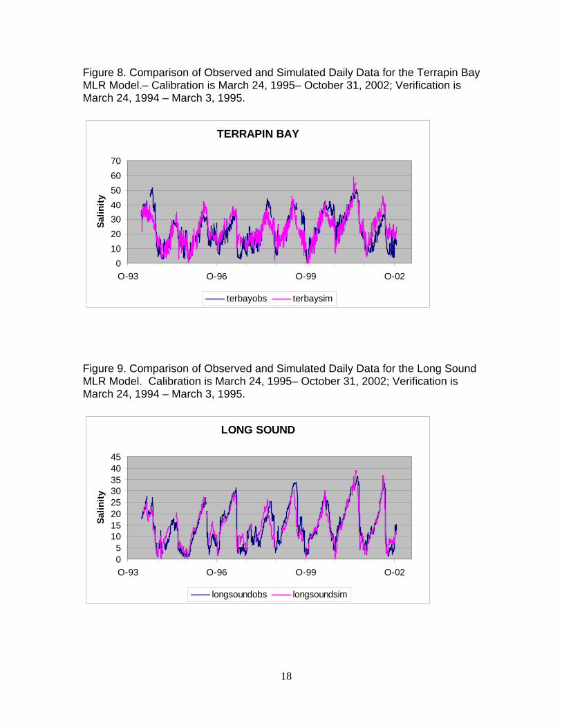
Figure 8. Comparison of Observed and Simulated Daily Data for the Terrapin Bay MLR Model.– Calibration is March 24, 1995– October 31, 2002; Verification is March 24, 1994 – March 3, 1995.

TERRAPIN BAY

010203040506070

O-93 O-96 O-99 O-02

Salin

ity

terbayobs terbaysim

Figure 9. Comparison of Observed and Simulated Daily Data for the Long Sound MLR Model. Calibration is March 24, 1995– October 31, 2002; Verification is March 24, 1994 – March 3, 1995.

LONG SOUND

05

1015202530354045

O-93 O-96 O-99 O-02

Salin

ity

longsoundobs longsoundsim

18

Figure 10. Comparison of Observed and Simulated Daily Data for the Whipray Basin MLR Model.Calibration is March 24, 1995– October 31, 2002; Verification is March 24, 1994 – March 3, 1995.

WHIPRAY BASIN

0

10

20

30

40

50

60

O-93 O-96 O-99 O-02

Salin

ity

whiprayobs whipraysim

Figure 11. Comparison of Observed and Simulated Daily Data for the Duck Key MLR Model.– Calibration is March 24, 1995– October 31, 2002; Verification is March 24, 1994 – March 3, 1995.

DUCK KEY

05

1015202530354045

O-93 O-96 O-99 O-02

Salin

ity

duckobs ducksim

19

Figure 12. Comparison of Observed and Simulated Daily Data for the Butternut Key MLR Model. Calibration is March 24, 1995– October 31, 2002; Verification is March 24, 1994 – March 3, 1995.

BUTTERNUT KEY

05

1015202530354045

O-93 O-96 O-99 O-02

Salin

ity

butternutobs butternutsim

Figure 13. Comparison of Observed and Simulated Data for the Taylor River MLR Model – Calibration is March 24, 1995 – October 31, 2002; Verification is March 24, 1994 – March 3, 1995.

TAYLOR RIVER

05

1015202530354045

O-93 O-96 O-99 O-02

Salin

ity

taylorriverobs taylorriversim

20

Figure 14. Comparison of Observed and Simulated Data for the Highway Creek MLR Model – Calibration is March 24, 1995 – October 31, 2002; Verification is March 24, 1994 – March 3, 1995.

HIGHWAY CREEK

05

10152025303540

O-93 O-96 O-99 O-02

Salin

ity

hiwaycreekobs hiwaycreeksim

Figure 15. Comparison of Observed and Simulated Data for the Little Blackwater Sound MLR Model – Calibration is March 24, 1995 – October 31, 2002; Verification is March 24, 1994 – March 3, 1995.

LITTLE BLACKWATER SOUND

05

1015202530354045

O-93 O-96 O-99 O-02

Salin

ity

ltblackwaterobs ltblackwatersim

21

Figure 16. Comparison of Observed and Simulated Data for the Bob Allen Key MLR Model – Calibration is September 9, 1998– October 31, 2002; Verification is September 9, 1997 – September 8, 1998.

BOB ALLEN KEY

0

10

20

30

40

50

O-93 O-96 O-99 O-02

Salin

ity

boballenobs boballensim

Figure 17. Comparison of Observed and Simulated Daily Data for the Garfield Bight MLR Model. Calibration is March 6, 1997 – December 31, 2002; Verification is March 6, 1996 – March 5, 1997.

GARFIELD BIGHT

010203040506070

O-93 O-96 O-99 O-02

Salin

ity

garbightobs garbightsim

22

Figure 18. Comparison of Observed and Simulated Daily Data for the Clearwater Pass MLR Model. Calibration is May 10, 1997 – December 31, 2002; Verification is May 10, 1996 – May 9, 1997.

CLEARWATER PASS

05

1015202530354045

O-93 O-96 O-99 O-02

Salin

ity

clearwaterobs clearwatersim

Figure 19. Comparison of Observed and Simulated Daily Data for the Whitewater Bay MLR Model. Calibration is August 27,1996 – December 31, 2002; Verification is August 27, 1995 – August 26, 1996.

WHITEWATER BAY

05

101520253035

O-93 O-96 O-99 O-02

Salin

ity

whitewaterobs whitewatersim

23

Figure 20. Comparison of Observed and Simulated Daily Data for the North River MLR Model. Calibration is March 6, 1997 – December 31, 2002; Verification is March 6, 1996 – March 5, 1997.

NORTH RIVER

05

101520253035

O-93 O-96 O-99 O-02

Salin

ity

norrivobs norrivsim

Figure 21. Comparison of Observed and Simulated Daily Data for the Gunboat Island MLR Model. Calibration is March 22, 1997 – December 31, 2002; Verification is March 22, 1996 – March 21, 1997.

GUNBOAT ISLAND

05

10152025303540

O-93 O-96 O-99 O-02

Salin

ity

gunboatobs gunboatsim

24

Figure 22. Comparison of Observed and Simulated Daily Data for the Shark River MLR Model. Calibration is January 1, 1997 – December 31, 2002; Verification is January 1, 1996 – December 31, 1996.

SHARK RIVER

05

1015202530354045

O-93 O-96 O-99 O-02

Salin

ity

sharkriverobs sharkriversim

25

D. Model Error Statistics The ability of the MLR salinity models to simulate the observed conditions can be evaluated using a number of error statistics. For this project, the statistics that were computed to measure model performance are described below.

1. Mean Square Error The Mean Square Error, or MSE, is defined as the square of the mean of the squares of all the errors, as follows:

2

1

)(1 ∑=

−=N

n

PON

MSE

2. Root Mean Square Error

The Root Mean Square Error is defined as:

RMS =1N

O(n) − P(n)( )2n=1

N

∑

The Root Mean Square Error is a weighted measure of the error where the largest deviations between observed and predicted values contribute most to this uncertainty statistic. This statistic has units that are the same as the observed and predicted values. It is thought to be the most rigorous tests of absolute error (Hamrick, 2003).

3. Adjusted – R2 The Coefficient of Multiple Determination (R2) is the most common measure of the explanatory capability of a model. It is defined as: R2 = Sum of Squares Regression/Sum of Squares Total, or = 1- (Sum of Squares Error/Sum of Squares Total) R2 measures the percentage reduction in the total variation of the dependent variable associated with the use of the set of independent variables that comprise the model (Neter, et al; 1990). When there are many variables in the model, it is common to use the Adjusted Coefficient of Multiple Determination (adj-R2), which is R2 divided by the associated degrees of freedom.

4. Mean Error The Mean Error is another measure of model uncertainty. It is defined as:

ME =1N

O(n ) − P(n)( )n=1

N

∑

26

where O=observed values, P=predicted values, and N= number of observations used to develop the model. Positive values of the mean error indicate that the model tends to over-predict, and negative values indicated that the model tends to under-predict (Hamrick, 2003.)

5. Mean Absolute Error The Mean Absolute Error is defined as:

MAE =1N

O(n) − P(n)

n=1

N

∑

Although the Mean Absolute Error tells nothing about over- or under-prediction, it is considered as another measure of the agreement between observed values and predicted values. It is preferred by some because it tends to cancel the effects of negative and positive errors, and is therefore less forgiving compared to the Mean Error (Hamrick, 2003).

6. Maximum Absolute Error The Maximum Absolute Error is defined as: MAX = maxO(n) − P(n) : n =1, N The Maximum Absolute Error is the largest deviation between observed and predicted values.

7. Nash-Sutcliffe Efficiency The Nash-Sutcliffe Efficiency is a measure of model performance that is similar to R2. It was first proposed for use with models in 1970 (Nash and Sutcliffe, 1970). It is defined as:

∑

∑

=

=

−

−−= N

n

N

n

OO

OPNSE

1

1

)(

)(1

The value of the NSE roughly corresponds to the percentage of variation that is explained by a model.

8. Relative Mean Error Relative measures of error are not as extreme as the absolute measures presented above. Relative error statistics provide a measure of the error relative to the observed value. The Relative Mean Error is defined as:

27

RME =O(n) − P(n)( )

n =1

N

∑

O(n)

n=1

N

∑

9. Relative Mean Absolute Error

The Relative Mean Absolute Error is defined as:

RMA =O(n) − P(n)

n=1

N

∑

O(n)

n=1

N

∑

Caution must be applied in the use of these two statistics when there can be small values of the observed and predicted variable, and when they can have both positive and negative signs (Hamrick, 2003).

10. Relative Mean Square Error The Relative Mean Square Error is not as prone to fouling by small values and/or the presence of both positive and negative values and is defined as (Hamrick, 2003):

RSE =O(n) − P(n)( )2

n=1

N

∑

O(n) − O ( )2 + P (n) − O ( )2( )n =1

N

∑

The Relative Mean Square Error has values between zero and one, with a model that predicts well having a Relative Mean Square Error close to zero. Table 3 presents a summary of the values of these statistics for the models that were developed as part of this project. Table 4 presents the uncertainty statistics for the IOP/CESI models that were previously developed (Marshall, 2003b). The relative model statistics were not generated for these models. The error statistics in Table 3 indicate that the new models, particularly those for the southwest Gulf coast north of Cape Sable, explain a relatively large percentage of the variation in salinity compared to some of the CESI / IOP models. The adjusted R2 values for the southwestern Gulf coast models range from 0.74 - 0.85, with Nash-Sutcliffe efficiencies of 0.88 – 0.92. The root mse and the mean absolute error are between 3 – 4 psu, meaning that estimation of point values produced by the models can be expected to have a potential error margin of 3 – 4 psu, on the average. As with all of the daily MLR salinity models, including the CESI / IOP models, the maximum absolute error is between 9 – 18 psu, which means that there is the potential for a point estimate to have an error this large.

28

Table 3. Comparison of Model Uncertainty Statistics for SES MLR Salinity Models Developed for this Project.

station

mean square error

root mse

adj R-sq

mean error

mean abs error

max abs error

relative mean error

relative mean abs error

relative mean

square error

Nash- Sutcliffe Effcy.

Garfield Bight 37.9 6.15 0.68 -0.36 4.75 21.1 -0.012 0.16 0.06 0.89 Clearwater Pass 11.60 3.40 0.85 -0.12 2.72 10.82 -0.01 0.16 0.08 0.85 Whitewater Bay 9.60 3.10 0.74 0.46 2.90 10.60 0.04 0.26 0.06 0.88 North River 14.30 3.80 0.77 0.56 3.23 17.92 0.08 0.45 0.04 0.92 Gunboat Island 11.50 3.40 0.85 1.03 3.02 13.28 0.09 0.27 0.05 0.89 Shark River 6.30 2.50 0.82 -0.11 2.02 9.11 0.00 0.08 0.06 0.89

Table 4. Comparison of Model Uncertainty Statistics for IOP / CESI MLR Salinity Models Developed Previously.

station

mean sq error (mse), psu2

root mse

(rmse), psu

adj R-sq

mean error, psu

mean abs

error, psu

max abs error, psu

Nash-Sutcliffe

Efficiency Joe Bay 25.8 5.1 0.75 -0.14 3.7 20.6 0.76

Little Madeira

Bay 40.1 6.4 0.65 -0.66 5.1 22.6 -0.96

Terrapin Bay 32.6 5.7 0.75 -0.99 5.4 5.4 0.67

Whipray Basin 7.2 2.7 0.8 0.11 2.2 10.1 0.77

Duck Key 9.7 3.1 0.71 -0.18 2.27 14.4 0.71 Butternut

Key 10.7 3.3 0.65 0.1 2.7 11.3 0.66

Long Sound 15 3.9 0.8 0.31 2.7 18.9 0.81 Taylor River 21.4 4.6 0.78 -0.49 3.6 22.9 0.78

Highway Creek 18.2 4.3 0.81 -0.95 3.7 17.7 0.76

Little Blackwater

Sound 14 3.7 0.75 -0.14 2.9 15.7 0.76

Bob Allen Key 7.2 2.7 0.79 0.3 2.1 9.2 0.81

29

However, high values of the absolute error generally occur at the stations that are most directly affected by the freshwater flows from the Everglades. Large residuals can occur at the end of the dry season when the wet season begins in an abrupt fashion, as shown by the plots comparing observed and simulated conditions. According to the mean error statistic, the Whitewater Bay, North River, and Gunboat Island models tend to over-predict, while the Clearwater Pass and Shark River models tend to under-predict. For Garfield Bight in north-central Florida Bay, the error statistics show that this new model is comparable to the southwestern Gulf coast models described above. The R2 value (0.68) is slightly lower, but the Nash-Sutcliffe Efficiency value is about the same (0.89). The root mse, mean absolute error, and maximum absolute error are also higher. The Garfield Bight model can be expected to produce point estimates that have an average potential error of between 5 – 6 psu. The mean error indicates that the Garfield Bight model under-predicts, and the relative mse shows that the model is expected to predict well. Taken as a whole, the error statistics show that the new southwestern Gulf coast models will likely predict better than the near-shore, central and eastern embayment models. The new southwestern Gulf coast models have similar error statistics as the models for the northeastern embayments, and also are similar in error statistics to the open-water models. The Garfield Bight model is similar to the other near-shore embayments in error structure, such as Terrapin Bay, Little Madeira Bay, and Joe Bay. All of these near-shore embayments have a characteristic wide variation in observed salinity, with high and low salinity daily average values that are typical during a year with average hydrologic conditions.

E. Florida Bay Analysis Discussion One task of this project was to utilize existing Florida Bay MLR salinity models and develop new Florida Bay models for the purpose of evaluating ICU water management alternatives. Eleven (11) existing CESI / IOP MLR salinity models were used for this analysis. Six (6) new MLR salinity models were developed, including a replacement model for the CESI / IOP models for North River, Garfield Bight. A total of seventeen (17) models were prepared for use with 2X2 Model output for various CERP alternatives and historical wind and sea surface elevation data to construct 36-year time series for evaluation of the water management scenarios. By adding the new models, additional temporal and spatial information about the salinity regime in Florida Bay and the southwestern Gulf coast has been gained, particularly at stations that are directly influenced by Shark Slough. The first models that were developed for the ENP CESI projects were models for stations in the near-shore embayments and in the central and eastern open water areas. In general, the salinity in the near-shore embayments (Joe Bay, Little Madeira Bay, and Terrapin Bay) is observed to be more variable on a day-to-day basis than the salinity at the open water stations. Because of this, the

30

development of MLR salinity models was more difficult and the R2 and Nash-Sutcliffe Efficiency values are slightly lower compared to the open water MLR salinity models. The Garfield Bight model is a new model developed for this project. The Garfield Bight model error statistics are similar to the other near-shore embayment models. In addition to the models for the near-shore embayments in Florida Bay, MLR salinity models were developed for several of the coastal creeks and open water sounds of extreme northeast Florida Bay and for Taylor River. Because the salinity at these stations is not as variable, in general, as the salinity in the near-shore embayments, the MLR salinity models are capable of explaining a higher percentage of observed salinity variability than the near-shore embayment models. R2 and Nash-Sutcliffe Efficiency values for these models are slightly higher than the values for the near-shore embayments. In a similar manner, the observed salinity for the stations located directly within the influence of Shark Slough discharge also has less variability day-to-day than salinity in the near-shore embayments of northeast and central Florida Bay. As a result, the MLR salinity models for these stations also explain a slightly higher percentage of variability. As was observed for the CESI / IOP models, Craighead Pond (CP) was the water level station that the SAS© stepwise linear regression process chose as the independent variable amongst all independent variables that consistently explained the most variation in salinity at the most stations. However, for a variety of reasons, it was deemed to also be important to include other variables in the models that may be “over-shadowed” by the influence of CP. For example, for the salinity stations in extreme northeast Florida Bay, EVER7 in the ENP “panhandle” was also a significant local variable, so the MLR salinity models were controlled as they were developed to include EVER7 as a local hydrologic indicator, usually in concert with CP or P33 as regional hydrologic indicators. In the models for the stations within the Shark Slough discharge influence, the model development was controlled to include P33 and exclude CP from these MLR salinity models. These three (3) Everglades water level stations (CP, P33, and EVER7) are considered to be the “primary” stations for MLR salinity modeling. In most cases there was also a second or third Everglades water level station that was of lesser significance than the primary stations, but still significant at the 99.9% significance level that was used as the threshold for inclusion in the model for the stepwise regression process. These secondary stations include EVER6, E146, R127, P35, NP62, NP206, and G3273. Additionally, in all models wind vectors were significant, and in most models the sea surface level measured at Key West was also a significant independent variable. The error statistics that were computed indicate that the MLR salinity models for the near-shore embayments can be considered to be good, if grading on a scale of

31

poor, fair, good, very good, and excellent. For the open water stations, the MLR salinity model for Whipray Basin and Bob Allen Key are good to very good, while the models for Duck Key and Butternut Key are good. The models for the coastal creeks and extreme northeast Florida Bay stations (Long Sound, Highway Creek, Little Blackwater Sound, and Taylor River) are considered to be very good. The MLR salinity models for the southwestern Gulf coast (North River, Gunboat Island, Shark River, Clearwater Pass, and Whitewater Bay) are considered to be very good. This grouping of similar models by goodness-of-fit statistics follows closely the similar-salinity groups presented in Orlando, et al (1998) from an archival salinity data set.

32

III. Barnes Sound and Manatee Bay Analysis

A. Study Area and Data

The area of study for this task includes Barnes Sound and Manatee Bay, two interconnected water bodies. These estuarine water bodies are considered to be a part of southern Biscayne Bay. In reality, Barnes Sound and Manatee Bay are distinct from both Biscayne Bay and northeast Florida Bay, being separated by Card Sound Road on the north from Biscayne Bay, and on the south by U.S. Highway No. 1 from Florida Bay. Orlando, et al (1998) designates Barnes Sound and Manatee Bay as a separate salinity zone. The Intracoastal Waterway (ICW) and a few highway culverts provide the hydraulic connection between Card Sound in Biscayne Bay and Long Sound, Little Blackwater Sound and Blackwater Sound in Florida Bay, as shown on Figure 1. Barnes Sound, Manatee Bay, and Card Sound are not located in either Biscayne Bay National Park or Everglades National Park. As can be seen from Table 1, the monitoring station for Barnes Sound is near Middle Key and is therefore named as such. The upstream drainage areas of Barnes Sound and Manatee Bay are part of the Everglades regional hydrologic system. However, because of their geographic location, historically these water bodies may have also been influenced by freshwater that was released from groundwater stored in the topographic high area of the Atlantic Coastal Ridge (on which the Miami metropolitan area is located) through several naturally occurring tidal creeks that drain the coastal marl prairie and mangrove fringe areas into Manatee Bay and Barnes Sound. Barnes Sound and Manatee Bay are now also affected at times by discharges from the C-111 Canal system into Manatee Bay near U.S. Highway No. 1 through the S-197 structure, which is operated by the South Florida Water Management District (SFWMD). While the S-197 structure was originally a free-flowing discharge, it was plugged and now only flows during periods of high water, which happens to some extent most normal or wet years. In recent years the discharge canal from S-18C to S-197 has been modified to encourage flow out of the discharge canal before it reaches S-197, thereby simulating natural sheet flow across the marl prairie and through the mangrove areas to the extent possible. Most of the independent variable data that were used for the development of the Manatee Bay and Middle Key (Barnes Sound) MLR salinity models are presented in Table 2, and are the same data as for the Florida Bay models. Additionally, for Manatee Bay and Middle Key model development, five new water level stations were added to the 14 stage stations that were used for the Florida Bay and southwest Gulf coast models. The stations were selected to provide additional independent variables for stage from within the vicinity of the upstream areas draining directly into Barnes Sound and Manatee Bay. The additional stage stations considered for inclusion in the MLR models were EVER1 (a/k/a SWEVER1), G1183, 196A, G580, and G3356. While EVER1 data are average

33

daily values like the original 14 stations, G1183, 196A, G580, and G3356 are USGS stations and the values used were maximum daily values.

B. Model Development Model development for the Manatee Bay and Middle Key (Barnes Sound) stations was completed in the same manner as was described previously for the Florida Bay analysis. However, the Manatee Bay and Middle Key models were controlled to include the stage station EVER1. It is desirable to include EVER1 in the Manatee Bay and Middle Key models because it is the only stage monitoring station in the triangular area enclosed by U.S. Highway No. 1 and Card Sound Road. The water level in the mangroves within ENP west of U.S. Highway No. 1 has been observed to be higher at times than the water level east of the road. Future improvements to water management may include additional culverts in the roads. Therefore, if at all possible, EVER1 needs to be an independent variable in the regression model. The correlation analysis showed that many of the independent variables are correlated with salinity at Manatee Bay and Middle Key. A notable exception is Key West water level, which was not highly correlated to salinity at either station. The lack of correlation with Key West water level is in direct contrast to the relatively high level of correlation with salinity that was seen in almost all of the Florida Bay and southwest Gulf coast stations. This is an indication of the isolation of Barnes Sound and Manatee Bay from exchange with the Atlantic Ocean, a situation that is obvious from Figure 2. Although the USGS maximum daily water levels from the additional stations were also correlated with salinity, the level of correlation was not high and ultimately they were eliminated as model parameters by the selective stepwise regression technique that was used. It was found that forcing the MLR salinity models to include EVER1 water level produced models that, in general, had lower R2 and Nash-Sutcliffe Efficiency values than the other Florida Bay and southwest Gulf coast MLR salinity models. While it was possible to produce models with goodness-of-fit statistics that had higher values, the models with better statistics did not include the EVER1 station. Therefore, similar to model development for the open water stations of Whipray Basin, Duck Key, Butternut Key, and Bob Allen Key, the salinity values in adjacent Long Sound and Little Blackwater Sound were tested in the models. The improvement to the R2 value and Nash-Sutcliffe Efficiency values (as well as other statistics) for both models was substantial when the salinity in the adjacent water bodies was included, resulting in models with R2 and Nash-Sutcliffe efficiency values that were comparable to the values generated by the other MLR salinity models that have been developed to-date. Therefore, the Middle Key MLR salinity model includes salinity at both Long Sound and Little Blackwater Sound, while the Manatee Bay model includes only Little Blackwater Sound salinity, along with other independent variables (including the water level at EVER1 for both models).

34

Because the Manatee Bay and Middle Key models include salinity as well as stage and wind, a two-step process will be used for simulation of salinity at these stations. Salinity at Long Sound and Little Blackwater Sound is simulated first using the MLR salinity models presented above. Modeled Long Sound and Little Blackwater Sound salinity are then used with other independent variables to produce simulations of Manatee Bay and Middle Key salinity. To determine if the two-step process was really an improvement, Pearson correlation coefficients were computed for the calibration / verification period for the best MLR salinity models for Manatee Bay and Middle Key using EVER1 (but not Long Sound and/or Little Blackwater Sound salinity), and for the models that also included Long Sound and Little Blackwater Sound salinity. It was confirmed that the two-step process with salinity produces simulations that were considerably better than the one-step simulations without salinity. Ultimately, the modified stepwise regression procedure produced acceptable MLR salinity models for Manatee Bay and Middle Key. The MLR salinity models that were produced are as follows: MIDDLE KEY = 23.4 - 1.2 CP - 2.2 EVER1 - 0.12 UWNDKW[lag2]

+ 0.1 UWNDMIA[lag2] + 0.16 LITTLE BLACKWATER[lag3] + 0.27 LONG SOUND

MANATEE BAY = 23.2 - 2.9 EVER1[lag2] - 1.65 CP[lag1]

- 0.22 UWNDKW - 0.17 UWNDKW[lag2] - 0.09 VWNDKW[lag1] + 0.09 UWNDMIA + 0.18 UWNDMIA[lag2] + 0.39 LITTLE BLACKWATER where LONG SOUND and LITTLE BLACKWATER SOUND are the salinity (observed or modeled) at the Long Sound and Little Blackwater Sound MMR monitoring stations.)

Daily verification plots are presented in Figures 22 and 23. Table 5 presents a summary of the values of the uncertainty statistics for the Manatee Bay and Middle Key models. Refer to the explanation of the uncertainty statistics in the Florida Bay analysis for further information on the computation methods for the statistics. Table 5 shows that the mean square error (mse) range of 6.67 to 9.5 compares very favorably to the range of mse values for the Florida Bay models (7.2 to 32.6), and similarly so for root mse. The mean error shows that the Middle Key model under-predicts slightly, while the Manatee Bay model over-predicts slightly. The mean absolute error values for all models are comparable to the lowest values for the Florida Bay models. Maximum Absolute Error values are similar to the values for the Florida Bay models.

35

Figure 23. Comparison of Observed and Simulated Daily Data for the Middle Key MLR Model. Calibration is March 24, 1995 – October 31, 2001; Verification is March 24, 1994 – March 3, 1995.

MIDDLE KEY

05

101520253035404550

O-93 O-96 O-99 O-02

Salin

ity

middle obs middle sim

Figure 24. Comparison of Observed and Simulated Daily Data for the Manatee Bay MLR Model. Calibration is March 24, 1995 – December 31, 2000; Verification is March 24, 1994 – March 3, 1995.

MANATEE BAY

05

10152025303540

O-93 O-96 O-99 O-02

Salin

ity

Manatee Bay obs Manatee Bay sim

36

Table 5. Comparison of Model Uncertainty Statistics for MLR Salinity Models

station

mean square error

root mse

adj R-sq

mean error

mean abs error

max abs error

relative mean error

relative mean abs error

relative mean

square error

Nash-SutcliffeEffcy.

Middle Key 6.88 2.60 0.74 -0.22 2.20 11.33 -0.01 0.09 0.16 0.71 Manatee Bay Stage 9.50 3.10 0.69 0.02 2.07 12.86 0.00 0.09 0.17 0.70

For the relative measures, the relative mean error, relative mean absolute error, and relative mean square error are comparable to the values computed for the Florida Bay models. The Nash-Sutcliffe efficiencies are in the middle of the range of values for the CESI / IOP models. The adjusted-R2 values for the models are also comparable to the values for the Florida Bay models. Overall, the error statistics show that the Manatee Bay and Middle Key MLR salinity models perform as good as the best / better Florida Bay models. However, individual residuals can sometimes be large, a characteristic of the Florida Bay models as well. C. Manatee Bay and Barnes Sound Discussion The development of useful MLR salinity models for Manatee Bay and Middle Key (Barnes Sound) proved to be more difficult than the development of MLR salinity models for the stations in Florida Bay and on the southwestern Gulf coast. MLR salinity models which simulate very well can be prepared for Manatee Bay and Middle Key using the primary stage stations (EVER7, CP, and P33) from the Florida Bay models. However, it is important that these models reflect to the extent possible the conditions that are specific to the Manatee Bay and Barnes Sound contributing drainage area and the isolated conditions of the open water bodies. The drainage area upstream of the shore of Manatee Bay and Barnes Sound is constrained by the physical barriers of U.S. Highway No.1 and Card Sound Road, with only a small number of culverts supplying a hydraulic connection to the panhandle marl prairie and mangrove areas to the west. The only water level monitoring station in the confined area is EVER1 (a/k/a SWEVER1), so it is desirable that the models include this stage station if possible. Manatee Bay and Barnes Sound are also mostly isolated from Florida Bay and the rest of Biscayne Bay except for the connection provided by the Intracoastal

37

Waterway, which relates these two water bodies to the Florida Bay stations of Little Blackwater Sound and Long Sound. This isolation is manifested in the lack of significant correlation at either Manatee Bay or Little Blackwater Sound to the variation in sea surface elevation as measured at Key West as was seen at almost every other MMR monitoring station. For these reasons and others, the approach to the development of MLR salinity models for Manatee Bay and Middle Key stations was somewhat different than the method for the development of MLR salinity models at the other stations, involving many trial-and-error attempts and iterations. It was noted that reasonable models could be developed that included EVER7 as the primary stage station. To complicate matters, if EVER7 was included in a model, EVER1 had to be excluded from the models due to cross-correlation effect conflicts. In order to obtain a reasonable R2 value, EVER1 had to be paired at least with Craighead Pond (CP) to produce minimally acceptable R2 and Nash-Sutcliffe Efficiency values that were still below the values for the Florida Bay models. Other data (USGS stage data) were investigated but no improvement was found. Finally, reasonable MLR salinity models were developed that utilized salinity in adjacent Long Sound and Little Blackwater Sound as independent variables, in addition to EVER1, CP, and wind parameters. At both stations the error statistics improved considerably with the addition of salinity in the adjacent bays. It is concluded that acceptable MLR salinity models have been prepared for Manatee Bay and Middle Key (Barnes Sound). The models are considered to be good to very good for daily salinity simulations, but not excellent. Compared to the previously prepared models for Florida Bay and the southwest Gulf coast, the error statistics are better than most except for the R2 and Nash-Sutcliffe Efficiency values. These two goodness-of-fit measures are hampered by the lack of the ability of the Manatee Bay and Middle Key models to simulate the lowest salinity values, likely a result of the S-197 discharges.

38

IV. ICU Runs and Performance Measures

A. General

The Florida Bay, southwest Gulf coast, and the Manatee Bay and Middle Key (Barnes Sound) models were used to simulate salinity at each of the modeled stations. A combination of observed values for wind and sea surface elevation parameters and Everglades water level values that had been estimated by the SFWMD 2X2 Model for the Interim CERP Update (ICU) evaluations were used. The 2X2 Model ICU runs (Version 5.4) that were used for simulations include:

• Natural System Model (NSM) 4.6.2, • 2000 CERP (a/k/a 2000 base), • 2050 CERP (a/k/a 2050 base), • CERP 0, • CERP 1, • CERP 1.05BS, and • CERP 1.05t8.

Details on the specifics of these runs can be found on the evergladesplan.org website.

B. Simulation Procedure

The simulation procedure utilizes synthetic data (in this case - water level (stage) in the Everglades drainage basin) with other observed data (wind and sea surface elevation) to produce long-term time series estimates of salinity. The simulations are back-casted (or hind-casted) simulations because the 2X2 Model output represents an estimate of the water level in the Everglades that would have been produced by the hydrologic conditions of the period 1965-2000 utilizing the specified water management practice alternatives. In other words, the 2X2 Model ICU simulations represent the response of the system had the specified water management practices (the ICU alternatives – CERP0, CERP1, etc.) been in place for the entire 1965-2000 period. The use of 36-year back-casted simulations provides salinity data for a variety of climatic conditions, including average rainfall years, wet years, dry years, extended wet periods, and extended drought periods. These simulations will allow ecologists to comprehensively assess the short- and long-term impacts on the salinity regimes that are produced by the various ICU water management alternatives. Restoration of the historical salinity regime, to the extent possible, is important to the restoration of the natural resources of the south Florida coastal estuaries, both flora and fauna. To begin the simulation process, the 2X2 Model output for stage was evaluated by comparing the simulated stage values with the observed data. 2X2 Model output data were obtained from the evergladesplan.org website for the Version 5.6

39

calibration / verification run for the 1996-2001 period. When these data are compared to observed values, some of the 2X2 Model stage output simulates the observed values at the water level monitoring stations used for model development relatively well, while other stage output does not simulate observed values satisfactorily for the purposes of performance measure evaluations. The three stations that are the primary independent variables for Florida Bay and the southwest Gulf coast models are CP (Craighead Pond), P33, and EVER7, because they explain the largest percentage of variability in salinity compared to the other stage data. For the Middle Key (Barnes Sound) and Manatee Bay models the primary station is EVER1. Other stage stations are also included in most salinity models, though they are considered to be secondary because they explain a lesser percentage of the variability in salinity, but are still statistically significant at a high level. The comparison plots between 2X2 Model output and the observed data for these four primary stations only are presented in Figures 25, 26, 27, and 28. As can be seen, the P33 simulations match the observed values well, while the EVER7, CP, and EVER1 2X2 Model simulations have an observable and relatively large bias given the range of the stage data. For example, the value of the bias for EVER7 is -0.9, which means that the 2X2 Model simulation is high than the observed data by an average of 0.9 feet. Behavior at the other (secondary) stations was similar. Therefore, it was recommended to the Southern Estuaries Sub-team and accepted that the 2X2 Model output be corrected by adding or subtracting the bias, as appropriate, from the simulated values before being used as input to the MLR salinity models. The 2X2 Model output that was obtained was in the form of ‘stage minus land surface elevation’, which is water depth. Prior to applying the bias correction, the 2X2 Model output was converted to elevation at the monitoring station location by adding the elevation of the ground surface at the station. Therefore, as used for these simulations, the 2X2 Model output data are only the basis for the time series that is input to the statistical models. The 2X2 Model data are considered to be reasonable representations of the stage variation within a particular 2X2 Model grid cell for a particular run, but not a point value estimate for a specific location at any time. To obtain a point value estimate for use in the MLR salinity models, the daily 2X2 Model value was first adjusted as described for the elevation at a specific well. Following the elevation adjustment, the bias as explained above is added or subtracted to give the stage time series that is used for MLR salinity simulations. Table 6 presents the adjustments that were made to the 2X2 Model output before use in the MLR salinity models.

40

Figure 25. Comparison Between 2X2 Model Output and Observed Data for Stage Station P33

5

5.5

6

6.5

7

7.5

8

8.5

Jan-96 Jan-97 Jan-98 Jan-99 Jan-00 Jan-01

P332X2P33

Figure 26. Comparison Between 2X2 Model Output and Observed Data for Stage Station EVER7.

Jan-98 Jan-97

4

3.5

3

2.5

2

1.5

1

0.5

0

-0.5 Jan-96

Ever72X2 Ever7

Jan-99 Jan-00 Jan-01

41

Figure 27. Comparison Between 2X2 Model Output and Observed Data for Stage Station CP.

-2

-1.5

-1

-0.5

0

0.5

1

1.5

2

2.5

3

3.5

Jan-96 Jan-97 Jan-98 Jan-99 Jan-00 Jan-01

CP2X2Cp

Figure 28. Comparison Between 2X2 Model Output and Observed Data for Stage Station SWEVER1.

-1.5

-1

-0.5

0

0.5

1

1.5

2

2.5

3

3.5

Jan-96 Jan-97 Jan-98 Jan-99 Jan-00 Jan-01

swever1swever1obs

42

Table 6. Adjustments that were made to the output of the 2X2 Model for use in the MLR salinity models for the ICU simulations.

Station ID

2X2 Cell No.

Station Elev, NGVD

96-2000 Bias

CP R4C20 0.36 -0.63 E146 R5C21 0.80 -0.29 EVER1 R8C28 1.30 0.04 EVER4 R8C25 2.34 0.03 EVER6 R6C26 1.28 -0.56 EVER7 R6C25 1.33 -0.89 G3273 R17C24 6.78 -0.25 NP206 R15C21 6.02 0.13 NP46 R7C17 1.64 -0.16 NP62 R11C17 2.19 -0.11 NP67 R7C22 1.64 -0.3 P33 R17C20 5.55 -0.01 P35 R12C15 1.18 0.19 P37 R6C20 1.59 -0.22 P38 R9C16 1.14 0.02 R127 R8C23 1.76 -0.16

C. ICU Salinity Simulations The MLR salinity models were utilized to simulate salinity for the following ICU water management alternatives: Natural System Model (NSM) 4.6.2 2000 CERP 2050 CERP CERP 0 CERP 1 CERP 1.05BS, and CERP 1.05t8. A plot of each simulation is provided in the Appendix in sections titled by the individual ICU run. D. Comparisons of ICU Runs There are a variety of methods available for comparing the MLR ICU salinity simulations. There has been much discussion at the Sub-team meetings and at other RECOVER committee meetings about the methods that should be used for evaluating the effects on Florida Bay, the southwest Gulf coast, and Manatee Bay

43

44

and Barnes Sound of water management scenarios with respect to salinity variation. One common statistic for comparison purposes is the annual mean value, which was computed for each station. Another statistic that was computed that allows a comparison of seasonal salinity variation is the monthly mean value. Monthly average plots using the 36-year simulations were made that present the average value for each ICU run. Each monthly average value is the mean of 36 years multiplied by 28, 29, 30, 31 days, or the number of value in a month when there were missing values. Additionally, the Sub-team developed some threshold-type values in an attempt to bracket the desired salinity variation at the primary stations. Even though thresholds have been used for other evaluations, there has been comment that the thresholds chosen will always suffer from claims that they were arbitrarily chosen. Therefore, this study used a method for evaluating ICU runs utilizing a somewhat more statistically based comparison procedure. The 25th and 75th quartile values were computed for each run and plotted for comparison amongst ICU alternatives. The 25th quartile is the highest salinity value for lowest 25% of the data, and the 75th quartile is the lowest value for the highest 25% of the data. These values have units of PSU. In an area that is considered to have elevated salinity values because of water management activities (an example is Whipray Basin), alternatives that have reduced 25th and 75th quartile values compared to current conditions are considered to be ecological improvements. In an area that is considered to be receiving too much fresh water which is reducing salinity values (an example is Manatee Bay), higher 25th and 75th quartile values compared to the existing conditions are thought to be ecological improvements. The 25th and 75th quartile values provide a measure of the range of the distribution of estimated salinity values due to a water management alternative, while the annual mean provides a measure of central tendency, with the monthly mean providing a seasonal comparison. The plots of the referenced statistics are presented below followed by a discussion of the findings from an evaluation of the statistics at each station.

Figure 29. Joe Bay

JOE BAY ANNUAL MEAN

11

12

13

14

15

cerp2

000

cerp2

050

cerp0

cerp1

cerp1

_05b

s

cerp1

_05t8

nsm4_

6_2

Salin

ity

Monthly Mean Values

0

5

10

15

20

25

30

1 2 3 4 5 6 7 8 9 10 11 12

cerp2000cerp2050cerp0cerp1cerp1_05bscerp1_05t8nsmlow90nsmup90

Figure 30. Little Madeira Bay

LITTLE MADEIRA BAY ANNUAL MEAN

1617181920212223242526

cerp2

000

cerp2

050

cerp0

cerp1

cerp1

_05b

s

cerp1

_05t8

nsm4_

6_2

Salin

ity

Monthly Mean Values

10

15

20

25

30

35

1 2 3 4 5 6 7 8 9 10 11 12

cerp2000cerp2050cerp0cerp1cerp1_05bscerp1_05t8nsmlow90nsmup90

JOE BAY 25TH QUARTILE

3

4

5

6

cerp2

000

cerp2

050

cerp0

cerp1

cerp1

_05b

s

cerp1

_05t8

nsm4_

6_2

Salin

ity

JOE BAY 75TH QUARTILE

17

18

19

20

21

cerp2

000

cerp2

050

cerp0

cerp1

cerp1

_05b

s

cerp1

_05t8

nsm4_

6_2

Salin

ity

LITTLE MADEIRA BAY 25TH QUARTILE

11121314151617181920

cerp2

000

cerp2

050

cerp0

cerp1

cerp1

_05b

s

cerp1

_05t8

nsm4_

6_2

Salin

ity

LITTLE MADEIRA BAY 75TH QUARTILE

212223242526272829

cerp2

000

cerp2

050

cerp0

cerp1

cerp1

_05b

s

cerp1

_05t8

nsm4_

6_2

Salin

ity

45

Figure 31. Terrapin Bay

TERRAPIN BAY ANNUAL MEAN

18

20

22

24

26

28

30

cerp2

000

cerp2

050

cerp0

cerp1

cerp1

_05b

s

cerp1

_05t8

nsm4_

6_2

Salin

ity

Monthly Mean Values

10

15

20

25

30

35

40

45

1 2 3 4 5 6 7 8 9 10 11 12

cerp2000cerp2050cerp0cerp1cerp1_05bscerp1_05t8nsmlow90nsmup90

Figure 32. Garfield Bight

GARFIELD BIGHT ANNUAL MEAN

262728293031323334

cerp2

000

cerp2

050

cerp0

cerp1

cerp1

_05b

s

cerp1

_05t8

nsm4_

6_2

Salin

ity

Monthly Mean Values

15

20

25

30

35

40

45

50

1 2 3 4 5 6 7 8 9 10 11 12

cerp2000cerp2050cerp0cerp1cerp1_05bscerp1_05t8nsmlow90nsmup90

TERRAPIN BAY 25TH QUARTILE

10

12

14

16

18

20

cerp2

000

cerp2

050

cerp0

cerp1

cerp1

_05b

s

cerp1

_05t8

nsm4_

6_2

Salin

ity

TERRAPIN BAY 75TH QUARTILE

24

26

28

30

32

34

36

cerp2

000

cerp2

050

cerp0

cerp1

cerp1

_05b

s

cerp1

_05t8

nsm4_

6_2

Salin

ity

GARFIELD BIGHT 25TH QUARTILE

20

21

22

23

24

25

26

cerp2

000

cerp2

050

cerp0

cerp1

cerp1

_05b

s

cerp1

_05t8

nsm4_

6_2

Salin

ity

GARFIELD BIGHT 75TH QUARTILE

323334353637383940

cerp2

000

cerp2

050

cerp0

cerp1

cerp1

_05b

s

cerp1

_05t8

nsm4_

6_2

Salin

ity

46

Figure 33. Long Sound

LONG SOUND ANNUAL MEAN

14

15

16

17

18

cerp2

000

cerp2

050

cerp0

cerp1

cerp1

_05b

s

cerp1

_05t8

nsm4_

6_2

Salin

ity

Monthly Mean Values

0

5

10

15

20

25

30

35

1 2 3 4 5 6 7 8 9 10 11 12

cerp2000cerp2050cerp0cerp1erp1_05bscerp1_05t8nsmlow90nsmup90

Figure 34. Little Blackwater Sound

LITTLE BLACKWATER SOUND ANNUAL MEAN

18

19

20

21

22

cerp2

000

cerp2

050

cerp0

cerp1

cerp1

_05b

s

cerp1

_05t8

nsm4_

6_2

Salin

ity

b. Monthly Mean Values

10

15

20

25

30

35

1 2 3 4 5 6 7 8 9 10 11 12

cerp2000cerp2050cerp0cerp1cerp1_05bscerp1_05t8nsmlow90nsmup90

LONG SOUND 25TH QUARTILE

6

7

8

9

10

cerp2

000

cerp2

050

cerp0

cerp1

cerp1

_05b

s

cerp1

_05t8

nsm4_

6_2

Salin

ity

LONG SOUND 75TH QUARTILE

20

21

22

23

24

cerp2

000

cerp2

050

cerp0

cerp1

cerp1

_05b

s

cerp1

_05t8

nsm4_

6_2

Salin

ity

LITTLE BLACKWATER SOUND 25TH QUARTILE

11

12

13

14

15

cerp2

000

cerp2

050

cerp0

cerp1

cerp1

_05b

s

cerp1

_05t8

nsm4_

6_2

Salin

ity

LITTLE BLACKWATER SOUND 75TH QUARTILE

23

24

25

26

27

28

cerp2

000

cerp2

050

cerp0

cerp1

cerp1

_05b

s

cerp1

_05t8

nsm4_

6_2

Salin

ity

47

Figure 35. Highway Creek

HIGHWAY CREEK ANNUAL MEAN

101112131415161718

cerp2

000

cerp2

050

cerp0

cerp1

cerp1

_05b

s

cerp1

_05t8

nsm4_

6_2

Salin

ity

b. Monthly Mean Values

0

5

10

15

20

25

30

35

1 2 3 4 5 6 7 8 9 10 11 12

cerp2000cerp2050cerp0cerp1cerp1_05bscerp1_05t8nsmlow90nsmup90

Figure 36. Taylor River

TAYLOR RIVER ANNUAL MEAN

5

6

7

8

9

10

cerp2

000

cerp2

050

cerp0

cerp1

cerp1

_05b

s

cerp1

_05t8

nsm4_

6_2

Salin

ity

b. Monthly Mean Values

0

5

10

15

20

25

1 2 3 4 5 6 7 8 9 10 11 12

cerp2000cerp2050cerp0cerp1cerp1_05bscerp1_05t8nsmlow90nsmup90

HIGHWAY CREEK 25TH QUARTILE

0

1

2

3

4

5

6

cerp2

000

cerp2

050

cerp0

cerp1

cerp1

_05b

s

cerp1

_05t8

nsm4_

6_2

Salin

ity

HIGHWAY CREEK 75TH QUARTILE

181920212223242526

cerp2

000

cerp2

050

cerp0

cerp1

cerp1

_05b

s

cerp1

_05t8

nsm4_

6_2

Salin

ity

TAYLOR RIVER 25TH QUARTILE

-1

0

1

cerp2

000

cerp2

050

cerp0

cerp1

cerp1

_05b

s

cerp1

_05t8

nsm4_

6_2

Salin

ity

TAYLOR RIVER 75TH QUARTILE

8

10

12

14

16

cerp2

000

cerp2

050

cerp0

cerp1

cerp1

_05b

s

cerp1

_05t8

nsm4_

6_2

Salin

ity

48

Figure 37. Clearwater Pass

CLEARWATER PASS ANNUAL MEAN

12131415161718192021

cerp2

000

cerp2

050

cerp0

cerp1

cerp1

_05b

s

cerp1

_05t8

nsm4_

6_2

Salin

ity

Monthly Mean Values

5

10

15

20

25

30

35

1 2 3 4 5 6 7 8 9 10 11 12

cerp2000cerp2050cerp0cerp1cerp1_05bscerp1_05t8nsmlow90nsmup90

Figure 38. Whitewater Bay

WHITEWATER BAY ANNUAL MEAN

56789

101112131415

cerp2

000

cerp2

050

cerp0

cerp1

cerp1

_05b

s

cerp1

_05t8

nsm4_

6_2

Salin

ity

Monthly Mean Values

0

5

10

15

20

25

1 2 3 4 5 6 7 8 9 10 11 12

cerp2000cerp2050cerp0cerp1cerp1_05bscerp1_05t8nsmlow90nsmup90

CLEARWATER PASS 25TH QUARTILE

6789

1011121314

cerp2

000

cerp2

050

cerp0

cerp1

cerp1

_05b

s

cerp1

_05t8

nsm4_

6_2

Salin

ity

CLEARWATER PASS 75TH QUARTILE

16171819202122232425

cerp2

000

cerp2

050

cerp0

cerp1

cerp1

_05b

s

cerp1

_05t8

nsm4_

6_2

Salin

ity

WHITEWATER BAY 25TH QUARTILE

4

5

6

7

8

9

10

cerp2

000

cerp2

050

cerp0

cerp1

cerp1

_05b

s

cerp1

_05t8

nsm4_

6_2

Salin

ity

WHITEWATER BAY 75TH QUARTILE

101112131415161718

cerp2

000

cerp2

050

cerp0

cerp1

cerp1

_05b

s

cerp1

_05t8

nsm4_

6_2

Salin

ity

49

Figure 39. North River

NORTH RIVER ANNUAL MEAN

0123456789

10

cerp2

000

cerp2

050

cerp0

cerp1

cerp1

_05b

s

cerp1

_05t8

nsm4_

6_2

Salin

ity

Monthly Mean Values

02468

101214161820

1 2 3 4 5 6 7 8 9 10 11 12

cerp2000cerp2050cerp0cerp1cerp1_05bscerp1_05t8nsmlow90nsmup90

Figure 40. Gunboat Island

GUNBOAT ISLAND ANNUAL MEAN

56789

101112131415

cerp2

000

cerp2

050

cerp0

cerp1

cerp1

_05b

s

cerp1

_05t8

nsm4_

6_2

Salin

ity

Monthly Mean Values

0

5

10

15

20

25

1 2 3 4 5 6 7 8 9 10 11 12

cerp2000cerp2050cerp0cerp1cerp1_05bscerp1_05t8nsmlow90nsmup90

NORTH RIVER 25TH QUARTILE

-1

0

1

2

3

4

5

cerp2

000

cerp2

050

cerp0

cerp1

cerp1

_05b

s

cerp1

_05t8

nsm4_

6_2

Salin

ity

NORTH RIVER 75TH QUARTILE

2

4

6

8

10

12

14

16

cerp2

000

cerp2

050

cerp0

cerp1

cerp1

_05b

s

cerp1

_05t8

nsm4_

6_2

Salin

ity

GUNBOAT ISLAND 25TH QUARTILE

-1

0

1

2

3

4

5

6

cerp2

000

cerp2

050

cerp0

cerp1

cerp1

_05b

s

cerp1

_05t8

nsm4_

6_2

Salin

ity

GUNBOAT ISLAND 75TH QUARTILE

6

8

10

12

14

16

18

20

cerp2

000

cerp2

050

cerp0

cerp1

cerp1

_05b

s

cerp1

_05t8

nsm4_

6_2

Salin

ity

50

Figure 41. Shark River

SHARK RIVER ANNUAL MEAN

18

20

22

24

26

28

cerp2

000

cerp2

050

cerp0

cerp1

cerp1

_05b

s

cerp1

_05t8

nsm4_

6_2

Salin

ity

b. Monthly Mean Values

1517192123252729313335

1 2 3 4 5 6 7 8 9 10 11 12

cerp2000cerp2050cerp0cerp1cerp1_05bscerp1_05t8nsmlow90nsmup90

Figure 42. Whipray Basin

WHIPRAY BASIN ANNUAL MEAN

303132333435363738

cerp2

000

cerp2

050

cerp0

cerp1

cerp1

_05b

s

cerp1

_05t8

nsm4_

6_2

Salin

ity

a. Monthly Mean Values

2527293133353739414345

1 2 3 4 5 6 7 8 9 10 11 12

cerp2000cerp2050cerp0cerp1cerp1_05bscerp1_05t8nsmlow90nsmup90

SHARK RIVER 25TH QUARTILE

14

16

18

20

22

24

cerp2

000

cerp2

050

cerp0

cerp1

cerp1

_05b

s

cerp1

_05t8

nsm4_

6_2

Salin

ity

SHARK RIVER 75TH QUARTILE

22

24

26

28

30

32

cerp2

000

cerp2

050

cerp0

cerp1

cerp1

_05b

s

cerp1

_05t8

nsm4_

6_2

Salin

ity

WHIPRAY BASIN 25TH QUARTILE

26

27

28

29

30

31

32

cerp2

000

cerp2

050

cerp0

cerp1

cerp1

_05b

s

cerp1

_05t8

nsm4_

6_2

Salin

ity

WHIPRAY BASIN 75TH QUARTILE

34

35

36

37

38

39

40

cerp2

000

cerp2

050

cerp0

cerp1

cerp1

_05b

s

cerp1

_05t8

nsm4_

6_2

Salin

ity

51

Figure 43. Duck Key

DUCK KEY ANNUAL MEAN

222324252627282930

cerp2

000

cerp2

050

cerp0

cerp1

cerp1

_05b

s

cerp1

_05t8

nsm4_

6_2

Salin

ity

b. Monthly Mean Values

1517192123252729313335

1 2 3 4 5 6 7 8 9 10 11 12

cerp2000cerp2050cerp0cerp1cerp1_05bscerp1_05t8nsmlow90nsmup90

Figure 44. Butternut Key

BUTTERNUT KEY ANNUAL MEAN

25

26

27

28

29

30

31

cerp2

000

cerp2

050

cerp0

cerp1

cerp1

_05b

s

cerp1

_05t8

nsm4_

6_2

Salin

ity

Monthly Mean Values

20222426283032343638

1 2 3 4 5 6 7 8 9 10 11 12

cerp2000cerp2050cerp0cerp1cerp1_05bscerp1_05t8nsmow90nsmup90

DUCK KEY 25TH QUARTILE

181920212223242526

cerp2

000

cerp2

050

cerp0

cerp1

cerp1

_05b

s

cerp1

_05t8

nsm4_

6_2

Salin

ity

DUCK KEY 75TH QUARTILE

26

27

28

29

30

31

32

cerp2

000

cerp2

050

cerp0

cerp1

cerp1

_05b

s

cerp1

_05t8

nsm4_

6_2

Salin

ity

BUTTERNUT KEY 25TH QUARTILE

21

22

23

24

25

26

27

cerp2

000

cerp2

050

cerp0

cerp1

cerp1

_05b

s

cerp1

_05t8

nsm4_

6_2

Salin

ity

BUTTERNUT KEY 75TH QUARTILE

27

28

29

30

31

32

33

cerp2

000

cerp2

050

cerp0

cerp1

cerp1

_05b

s

cerp1

_05t8

nsm4_

6_2

Salin

ity

52

Figure 45. Bob Allen Key

BOB ALLEN KEY ANNUAL MEAN

30

31

32

33

34

35

36

cerp2

000

cerp2

050

cerp0

cerp1

cerp1

_05b

s

cerp1

_05t8

nsm4_

6_2

Salin

ity

b. Monthly Mean Values

25272931333537394143

1 2 3 4 5 6 7 8 9 10 11 12

cerp2000cerp2050cerp0cerp1cerp1_05bsncerp1_05t8nsmlow90nsmup90

Figure 46. Manatee Bay

MANATEE BAY ANNUAL MEAN

22

23

24

25

26

cerp2

000

cerp2

050

cerp0

cerp1

cerp1

_05b

s

cerp1

_05t8

nsm4_

6_2

Salin

ity

Monthly Mean Values

1517192123252729313335

1 2 3 4 5 6 7 8 9 10 11 12

cerp20002050cerp0cerp1cerp1_05bscerp1_05t8nsmup90nsmlow90

BOB ALLEN KEY 25TH QUARTILE

26

27

28

29

30

31

32

cerp2

000

cerp2

050

cerp0

cerp1

cerp1

_05b

s

cerp1

_05t8

nsm4_

6_2

Salin

ity

BOB ALLEN KEY 75TH QUARTILE

32

33

34

35

36

37

38

cerp2

000

cerp2

050

cerp0

cerp1

cerp1

_05b

s

cerp1

_05t8

nsm4_

6_2

Salin

ity

MANATEE BAY 25TH QUARTILE

17

18

19

20

21

cerp2

000

cerp2

050

cerp0

cerp1

cerp1

_05b

s

cerp1

_05t8

nsm4_

6_2

Salin

ity

MANATEE BAY 75TH QUARTILE

25

26

27

28

29

30

cerp2

000

cerp2

050

cerp0

cerp1

cerp1

_05b

s

cerp1

_05t8

nsm4_

6_2

Salin

ity

53

Figure 47. Middle Key

MIDDLE KEY ANNUAL MEAN

24

25

26

27

28

cerp2

000

cerp2

050

cerp0

cerp1

cerp1

_05b

s

cerp1

_05t8

nsm4_

6_2

Salin

ity

MIDDLE KEY 25TH QUARTILE

19

20

21

22

23

cerp2

000

cerp2

050

cerp0

cerp1

cerp1

_05b

s

cerp1

_05t8

nsm4_

6_2

Salin

ity

Monthly Mean Values MIDDLE KEY 75TH QUARTILE

28

29

30

31

32

cerp2

000

cerp2

050

cerp0

cerp1

cerp1

_05b

s

cerp1

_05t8

nsm4_

6_2

Salin

ity

15

20

25

30

35

40

1 2 3 4 5 6 7 8 9 10 11 12

cerp2000cerp2050cerp0cerp1cerp1_05bscerp1_05t8nsmup90nsmlow90

54

E. ICU Runs Discussion The purpose for preparing the 36-year simulations is to assist the Southern Estuaries Sub-team in determining which of the ICU runs produces salinity values that are the closest to “restoration conditions”, and which do not meet that goal. The meaning of “restoration conditions” has not been completely defined, and restoration conditions are different throughout the bay. Certain water bodies have been identified as important for ecological purposes, including Joe Bay, Little Madeira Bay, Terrapin Bay, and Garfield Bight in Florida Bay; North River on the southwest Gulf coast, and Barnes Sound / Manatee Bay between Florida Bay and Biscayne Bay. Performance measures have been or are in the process of being established for these primary water bodies so the performance of a particular run can be compared to a standard or threshold value. The other stations for which MLR salinity models have been developed may not be formally identified for performance measures, but they are important for filling-out the salinity picture. Additionally, because there are now more stations than just the primary water bodies with MLR salinity models, it is now possible to consider setting performance measures for some of these areas, such as Whipray Basin or Clearwater Pass and Whitewater Bay. The additional MLR salinity models allow the spatial resolution of the ICU evaluation to be improved. One method of evaluating ICU runs that has been discussed at many meetings related to CERP is the use of the Natural System Model output (NSM 4.6.2) as the basis for a “restoration condition”. For a number of reasons, there are varying levels of confidence in the NSM 4.6.2 output, even though there is little, if any observed data for comparison before there were alterations to the hydrology through water management projects. However, NSM 4.6.2 output is available to create daily salinity simulations at all stations over the 36-year period. Therefore, in order to demonstrate a scoring methodology to determine the best performing water management alternative, the NSM 4.6.2 simulations were used to make a comparison, as shown in Figures 25 through 47. Taking the NSM 4.6.2 comparisons as a whole, this analysis suggests that additional work needs to be done on water deliveries to the Everglades. The fact that few runs at a few stations met the NSM 4.6.2 salinity regime (located mostly where the C-111 discharges are supplied) and the fact that most of the violations occurred during the dry season says that there is not enough water being delivered to Taylor Slough and held in storage during the wet season and carried into the dry season. The extreme northeastern corner of the Bay appears to fare a little better, in general, than the other areas, when NSM 4.6.2 is used as the basis for comparison to the CERP water management alternatives. In contrast, the ICU alternative schemes create high salinity conditions relative to NSM 4.6.2 at Garfield Bight and Terrapin Bay, but still cause conditions that are fresher than NSM 4.6.2 at Middle Key (Barnes Sound) and Manatee Bay. Clearwater Pass

55

and Whitewater Bay experience higher-than-NSM 4.6.2 salinities from the examined CERP runs. North River, Gunboat Island and Shark River along the western side of the Park also are estimated to have high salinity regimes compared to NSM 4.6.2. For the central part of the Bay and at the open water stations, Whipray Basin is affected by the higher salinities of Garfield Bight and Terrapin Bay, while Duck Key and Butternut Key are affected similarly but to a lesser extent, with Bob Allen also behaving in a like manner. A further evaluation was performed using the Craighead Pond water level. Figure 48 shows the difference that exists between water levels at Craighead Pond produced by the NSM 4.6.2 run and those produced by CERP 2000 and CERP 0 runs. In general the CERP 0 differences are less. However, maximum differences of greater than one foot for CERP 2000 and about 0.75 feet occur at the end of the wet season most years. At other times the differences are about 0.25 feet, a little less for CERP 0 compared to CERP 2000. If NSM 4.6.2 is estimating low on Everglades water levels, then this CP analysis suggests that a further increase in stored water (1 foot or more on the average) is needed to achieve restoration conditions beyond that needed to meet NSM 4.6.2. An analysis done by Pitts, et al (draft, 2005) of literature associated with paleoecological investigations within the study area concluded that NSM MLR salinity model simulations were estimating salinity ranges that were higher than the paleo-records indicate for the pre-drainage (before 1900) periods. In Manatee Bay, comparisons to sediment records indicate that the NSM output is 5-15 psu higher, with the largest deviation seen in the wet season. In Whipray Basin, the same comparison shows that the salinity in Whipray Basin was about 10 psu lower historically than NSM indicates. For Joe Bay, the deviation is about 5 psu. Therefore, it appears that the use of NSM output to estimate pre-drainage conditions may not be providing an accurate picture. In summary, this analysis, based on a comparison of a number of ICU runs to NSM 4.6.2 conditions simulated by the MLR salinity models, indicates that none of the water management scenarios evaluated meets the NSM 4.6.2 basis adequately at most stations. The additional analysis using only the water levels simulated by the 2X2 Model at Craighead Pond indicate that additional water deliveries are needed to increase the water depth at CP by about 0.75 feet at the end of the dry season just to meet NSM 4.6.2 levels. However, this estimate would be considered to be too low by many who do not have confidence in the NSM 4.6.2 simulations.

56

Figure 48. Difference in Water Surface Elevation at Craighead Pond (CP) for NSM 4.6.2, and CERP2000 and CERP0 Produced by MLR Salinity Models

-1

-0.5

0

0.5

1

1.5

2

M-64 M-69 M-74 A-79 A-84 A-89 A-94 A-99

Diff

eren

ce, f

t.

NSM-2000CERP NSM-CERP0

57

V. Post-processing Activities

The Interagency Modeling Center (IMC) located at the South Florida Water Management District office in West Palm prepared computer code using the MLR salinity models presented herein. Future CERP water delivery alternative runs can be examined by having the IMC prepare salinity simulations for the evaluators in the same manner as is presented herein. The IMC code produces the same daily simulations as were produced for this study because the same salinity models are used. As a post-processing activity, a utility was developed by the IMC that will create annual mean, quartile, and monthly mean plots, and perhaps other comparative measures. While the IMC is using a computer coding language that is different than the SAS© code, the procedures used by the IMC are similar to the steps required to use the models in SAS©. The first step undertaken by the IMC was to prepare the computer code that contains the models. The IMC contractor that prepared the code was Michael Martin, with assistance from Hong Xu, and oversight by Jose Otero, all at SFWMD office in West Palm Beach, Florida. To initiate the process, SAS © code and MLR salinity model simulation data were provided by ECT to the IMC. ECT met with IMC representatives on three occasions to discuss progress. While the code was being written there was close coordination between the two groups. A quality assurance check was performed by the IMC comparing the output from the ECT SAS programs with the output from the IMC code.

58

VI. References Everglades National Park. 1997a. Everglades National Park Marine Monitoring Network 1994 Data Summary. Everglades National Park, Homestead, Florida. 67 pp. Everglades National Park. 1997b. Everglades National Park Marine Monitoring Network 1995 Data Summary. Everglades National Park, Homestead, Florida. 67 pp. Hamrick, J.M. 2003. Florida Bay Hydrodynamic and Salinity Model Analysis. South Florida Water Management District. West Palm Beach, Florida. 20-22. Marshall III, F.E. 2005. Using Statistical Models to Simulate Salinity Variability in Estuaries. In Estuarine Indicators, S. A. Bortone, Editor. CRC Press. Boca Raton, Florida. Pp 33-52. Marshall III, F. E.; D. Smith; and D. Nickerson. 2004. Using Statistical Models to Simulate Salinity Variation and Other Physical Parameters in North Florida Bay. Cetacean Logic Foundation, Inc. New Smyrna Beach, Florida. 36 pp. Marshall III, F. E.; D. Smith; and D. Nickerson. 2003a. Salinity Simulation Models for North Florida Bay Everglades National Park. Cetacean Logic Foundation, Inc. New Smyrna Beach, Florida. 41 pp. Marshall III, F. E. 2003b. IOP Salinity Analysis Using Statistical Models. Cetacean Logic Foundation, Inc. New Smyrna Beach, Florida. 35 pp. Nash, J. E. and J. V. Sutcliffe. 1970. River Flow Forecasting Using Conceptual Models Part I – A Discussion of Principles. Journal of Hydrology. Vol. 10, pp 282 – 290. North-Holland Publishing Co., Amsterdam, Holland. Neter, J.; W. Wasserman; M. H. Kutner. 1990. Applied Linear Statistical Models. Richard D. Irwin, Inc. Boston, Massachusetts. Orlando, S.P., Jr.; M.B. Robblee; C. J. Klein. 1998. Salinity Characteristics of Florida Bay: A Review of Archived Data Set (1955-1995). National Oceanographic and Atmospheric Administration, Office of Ocean Resources Conservation and Assessment, Silver Spring Maryland. 32 pp. Pandit, A.; C. El-Khazen; S.P. Sivaramapilli. 1991. Estimation of Hydraulic Conductivity Values in a Coastal Aquifer. Groundwater. Vol. 29, No.2. pp 175-180. Pitts, P.; D. Hallac; D. Deis. Draft, 2005. Establishing Targets for Salinity in Florida’s Southern Estuaries. Southern Estuaries Sub-team of RECOVER.

59

Smith, D. 1997. Everglades National Park Marine Monitoring Network 1996 Data Summary. Everglades National Park, Homestead, Florida. 94 pp. Smith, D. 1998. Everglades National Park Marine Monitoring Network 1997 Data Summary. Everglades National Park, Homestead, Florida. 100 pp. Smith, D. 1999. Everglades National Park Marine Monitoring Network 1998 Data Summary. Everglades National Park, Homestead, Florida. 100 pp. Smith, D. 2001. Everglades National Park Marine Monitoring Network 1999 Data Summary. Everglades National Park, Homestead, Florida. 65 pp.

60

61

APPENDIX