reciprocal-wedge transform : a space-variant image...
TRANSCRIPT

RECIPROCAL-WEDGE TRANSFORM:
A SPACE-VARIANT IMAGE REPRESENTATION
Frank C. H. Tong
B.Sc. Chinese University of Hong Kong 1983
M.Sc. Simon Fraser University 1987
A THESIS SUBMITTED IN PARTIAL FULFILLMENT
OF THE REQUIREMENTS FOR THE DEGREE OF
DOCTOR OF PHILOSOPHY in the School
of
Computing Science
@ Frank C. H. Tong 1995
SIMON FRASER UNIVERSITY
August 1995
All rights reserved. This work may not be
reproduced in whole or in part, by photocopy
or other means, without the permission of the author
Name:
Degree:
Title of thesis:
APPROVAL
Frank C. H. Tong
Doctor of Philosophy
Reciprocal-Wedge Transform: A Space-variant Image Representation
Examining Committee: Dr. Veronica Dahl
Chair
Dr. Ze-Nian Li (Thesis Advisor) Associate Professor, Computing Science
Dr. ~ r i a n V. ~ u n t Professor, Computing Science
Dr. Tom Ca,lvert Professor, Computing Science
Dr. Kamal Gupta (Internal Examiner) Associate Professor, Engineering Science
Dr. Steven L. Tanimoto (External Examiner) Professor, Computer Science University of Washington
Date Approved:

PARTIAL COPYRIGHT LICENSE
I hereby grant to Simon Fraser Universi the right to lend my
t' 7 thesis, pro'ect or extended essay (the title o which is shown below) to users o the Simon Fraser University Library, and to make partial or single co ies only for such users or in response to a request from the li i! rary of any other university, or other educational institution, on its own behalf or for one of its users. I further agree that permission for multiple copying of this work for scholarly purposes may be granted by me or the Dean of Graduate Studies. It is understood that copying or publication of this work for financial gain shall not be allowed without my written permission.
Author: (signature)
(date)

Abstract
The problems in computer vision have traditionally been approached as recovery prob-
lems. In active vision, perception is viewed as an active process of exploratory, probing
and searching activities rather than a passive re-construction of the physical world.
To facilitate effective interaction with the environment, a foveate sensor coupled with
fast and precise gaze control mechanism becomes essential for active data acquisition.
In this thesis, the Reciprocal-Wedge Transform (RWT) is proposed as a space-
variant image model. The RWT has its merits in comparison with other alternative
foveate sensing models such as the log-polar transform. The concise matrix repre-
sentation makes it enviable for its simplified computation procedures. Similar to the
log-polar transform, the RWT facilitates space-variant sensing which enables effective
use of variable-resolution data and the reduction of the total amount of the sensory
data. Most interestingly, its property of anisotropic mapping yields variable resolu-
tion primarily in one dimension. Consequently, the RWT preserves linear features
and performs especially well on translations in the images.
A projective model is developed for the transform, lending it to potential hardware
implementation of RWT projection cameras. The CCD camera for the log-polar
transform requires sensing elements of exponentially varying sizes. In contrast, the
RWT camera achieves variable resolution with oblique image plane projection, thus

alleviating the need for non-rectangular tessellation and sensitivity scaling on the
sensing elements. A camera model making use of the available lens design techniques
is investigated.
The RWT is applied to motion analysis and active stereo to illustrate the effec-
tiveness of the image model. In motion analysis, two types of motion stereo are
investigated, namely, longitudinal and lateral motion stereo. RWT motion stereo al-
gorithms are developed for linear and circular ego motions in road navigation, and
depth recovery from moving parts on an assembly belt. The algorithms benefit from
the perspective correction, linear feature preservation and efficient data reduction of
the RWT.
The RWT imaging model is also shown to be suitable for fixation control in active
stereo. Vergence and versional eye movements and scanpath behaviors are studied.
A computational interpretation of stereo fusion in relation to disparity limit in space-
variant imagery leads to the development of a computational model for binocular
fixation. The unique oculomotor movements for binocular fixation observed in human
system appears natural to space-variant sensing. The vergence-version movement
sequence is implemented for an effective fixation mechanism in RWT imaging. An
interactive fixation system is simulated to show the various modules of camera control,
vergence and version. Compared to the traditional reconstructionist approach, active
behavior is shown to be plausible.

Acknowledgements
My foremost gratitude goes to my thesis advisor, Dr. Ze-Nian Li, for his constant sup-
port and encouragement. I have learned many things from Ze-Nian during the course
of my working with him. I have learned from his persistence and industriousness as
a researcher. However, I admire most his knowledge and vision.
My deepest gratitude also goes to Dr. Brian Funt. I thank him for introducing
me to the area of computer vision. His inspiring suggestions have always been most
valuable. I would also like to thank Dr. Tom Calvert for being on my advisory
committee. I am grateful for his generosity with his time and comments. My thanks
also go to Dr. Kamal Gupta. He is my professor, and he is also my friend. His
thoroughness in reviewing my thesis is much appreciated.
I also owe my gratitude to Dr. Steven Tanimoto. I feel grateful to him for being
my external examiner. He has been very generous with both his time and helpful
comments. Steve is very knowledgeable in the area. His acceptance of my thesis
makes me feel I have accomplished something valuable.
I would like to express my appreciation to Dr. Woshun Luk. His constant concern
and encouragement are much appreciated. I am also thankful to Gray Hall for help
with the proof-reading.
My thanks also go to many of the graduate students. In particular, I would like to

thank Graham Finlayson for the interesting and inspiring discussions. Carlos Wong
and Xao Ou Ren shared the same office with me. I thank them for the refreshing
chats that kept me going even in the most boring days.
I also thank the entire staff of the Computing Science department. We are lucky
to have a crew of supporting staff who are so friendly and helpful. They indeed have
made a viable environment throughout my stay.
I owe all my accomplishments to my parents. They worked so hard to raise a
family of eight, yet they still supported us through school. It was not easy for them.
Finally, and by no means least, I want to acknowledge the support of my wife, Mimi
Kao. This thesis could not be possible without her caring and encouragement.

Contents
... Abstract 111
Acknowledgements v
1 Introduction 1
. . . . . . . . . . . . . . . . . . . . 1.1 Active Vision and Foveate Sensors 2
. . . . . . . . . . . . . . . . . . . . . . . 1.2 Reciprocal-Wedge Transform 4
. . . . . . . . . . . . . . . . . . . . . 1.3 Motion Stereo in RWT Domain 6
. . . . . . . . . . . . . . . . . . . 1.4 Active Fixation using RWT Sensor 7
. . . . . . . . . . . . . . . . . . . . . . . . . . . . . . 1.5 Thesis Overview 9
2 Survey 10
. . . . . . . . . . . . . . . . . . . . . . . . . . . . . . . 2.1 Active Vision 10
. . . . . . . . . . . . . . . . . . . . . . . . . . . 2.2 Log-polar Transform 14
. . . . . . . . . . . 2.2.1 Logarithmic mapping from retina to cortex 14
. . . . . . . . . . . . . . . . . . . . . . . 2.2.2 The retina-like sensor 19
. . . . . . . . . . . . . . . . . . . . . . . 2.2.3 Space-variant sensing 20
. . . . . . . . . . . . . . . . . . 2.2.4 Form invariant image analysis 22
. . . . . . . . . . . . . . . . . . . . . . . . . . . . 2.3 Binocular Fixation 23

2.3.1 Stereopsis . . . . . . . . . . . . . . . . . . . . . . . . . . . . . 23
2.3.2 Fixation . . . . . . . . . . . . . . . . . . . . . . . . . . . . . . 24
2.3.3 Oculomotor model . . . . . . . . . . . . . . . . . . . . . . . . 26
2.4 Advances in Stereo Verging Systems . . . . . . . . . . . . . . . . . . . 29
2.5 Non-frontal Imaging . . . . . . . . . . . . . . . . . . . . . . . . . . . 32
2.6 Directions in Active Vision Research . . . . . . . . . . . . . . . . . . 33
3 Reciprocal-Wedge Transform 35
3.1 The Mathematical Model . . . . . . . . . . . . . . . . . . . . . . . . . 35
3.1.1 Matrix notation . . . . . . . . . . . . . . . . . . . . . . . . . . 37
3.1.2 Remedy to singularity . . . . . . . . . . . . . . . . . . . . . . 38
3.1.3 The RWT View-of- World . . . . . . . . . . . . . . . . . . . . . 40
3.2 Transformation on Linear Structures . . . . . . . . . . . . . . . . . . 44
3.2.1 Preservation of linear features . . . . . . . . . . . . . . . . . . 44
3.2.2 Line detection using the Hough transform . . . . . . . . . . . 45
3.3 Anisotropic Space-Variant Resolution . . . . . . . . . . . . . . . . . . 46
3.4 Pyramidal Implementation . . . . . . . . . . . . . . . . . . . . . . . . 48
3.4.1 Pyramidal mapping . . . . . . . . . . . . . . . . . . . . . . . . 49
3.4.2 Pyramidal reduction . . . . . . . . . . . . . . . . . . . . . . . 50
3.4.3 Local RWT transformation . . . . . . . . . . . . . . . . . . . . 52
4 Camera Model 55
. . . . . . . . . . . . . . . . . . . . . . . 4.1 The RWT Projective Model 55
4.2 Non-Paraxial Focusing . . . . . . . . . . . . . . . . . . . . . . . . . . 58
4.2.1 The RWT lens . . . . . . . . . . . . . . . . . . . . . . . . . . 59
4.3 Projecting the Singularity . . . . . . . . . . . . . . . . . . . . . . . . 62
... V l l l

4.3.1 U-plane projection . . . . . . . . . . . . . . . . . . . . . . . . 63
4.3.2 V-plane projection . . . . . . . . . . . . . . . . . . . . . . . . 64
4.3.3 Displaced-center projection . . . . . . . . . . . . . . . . . . . 66
4.4 A Prototype RWT Camera . . . . . . . . . . . . . . . . . . . . . . . . 68
4.4.1 Periscopic lens design . . . . . . . . . . . . . . . . . . . . . . . 68
4.4.2 Design of the RWT camera . . . . . . . . . . . . . . . . . . . 69
. . . . . . . . . . . . . . . . . . . . . . . . . . . . 4.5 Optical Simulations 73
5 Applications of RWT Mapping 78
5.1 RWT Imaging in Road Navigation . . . . . . . . . . . . . . . . . . . . 78
5.1.1 Perspective inversion by RWT . . . . . . . . . . . . . . . . . . 79
. . . . . . . . . . . . . . . . . . . . . . . . . . . . . . . 5.1.2 Results 81
5.2 Depth from Ego Motion . . . . . . . . . . . . . . . . . . . . . . . . . 82
. . . . . . . . . . . . . . . . . . . . . . . . . . . 5.2.1 Motion stereo 82
5.2.2 Longitudinal motion stereo . . . . . . . . . . . . . . . . . . . . 83
5.2.3 Lateral motion stereo . . . . . . . . . . . . . . . . . . . . . . . 90
5.2.4 Search in the epipolar plane . . . . . . . . . . . . . . . . . . . 93
5.2.5 Experimental results . . . . . . . . . . . . . . . . . . . . . . . 95
6 Active Stereo 102
6.1 Binocular Vision in Space-variant Sensing . . . . . . . . . . . . . . . 102
6.1.1 Panum's fusional area . . . . . . . . . . . . . . . . . . . . . . 103
6.2 Computational Model for Binocular Fixation . . . . . . . . . . . . . . 106
6.2.1 Fusional range in RWT . . . . . . . . . . . . . . . . . . . . . . 106
6.2.2 Fixation mechanism . . . . . . . . . . . . . . . . . . . . . . . 111
6.3 Binocular Fixation using RWT Images . . . . . . . . . . . . . . . . . 113

. . . . . . . . . . . . . . . . . . . . . . 6.3.1 Disparity computation 115
. . . . . . . . . . . . . . . . . . . . . . . . . 6.3.2 Fixation transfer 117
. . . . . . . . . . . . . . . . . . . . . . . . . . . 6.3.3 A system view 119
. . . . . . . . . . . . . . . . . . . . 6.3.4 A scanpath demonstration 125
7 Conclusions and Discussion 131
. . . . . . . . . . . . . . . . . . . . . . . . . . . . . . . 7.1 Contributions 131
. . . . . . . . . . . . . . . . . . . . . . . . . . . . . . 7.2 Future research 133
Bibliography 151

List of Figures
. . . . . . . . 2.1 Images of straight lines under the logarithmic mapping 18
. . . . . . . . . . . . . . . . . . . 2.2 The oculomotor map of visual space 27
2.3 The sequence of events in a mixed version and vergence movement . . 28
. . . . . . . . . . . . . . . . . . . . . The Reciprocal-Wedge transform 36
. . . . . . . . . . . . . . . . Geometric transformations on u-v images 39
. . . . . . . . . . . . . . . . . . . . . . . . . The RWT View.of.World 41
The Reciprocal-Wedge transform under the RWT VOW . . . . . . . . 43
. . . . . . . . The duality relationship of linear structures in the RWT 46
. . . . . . . . . . . . . . . . Mapping the image space to the pyramid 49
. . . . . . . . . . . . . . . . . . . . . . . The pyramidal reduction step 51
. . . . . . . . . . . . . . . . . . . . . . The RWT transformation step 52
. . . . . . . . . . . . . . . . . . . . . . 4.1 A perspective projection model 56
. . . . . . . . . . . . . . . . . 4.2 A rudimentary RWT projection camera 57
4.3 The focusing problem of the sideway-positioned RWT projection plane . 58
. . . . . . . . . . . . . . . . . 4.4 Optical principle in tilted plane focusing 60
. . . . . . . . . . . . . . . . . . . . . . . . . 4.5 The prototype RWT lens 62
. . . . . . . . . . . . . . . . . . . . . . . . . . . . . 4.6 U-plane projection 63

. . . . . . . . . . . . . . . . . . . . . . . . . . . . . 4.7 V-plane projection
. . . . . . . . . . . . . . . 4.8 Geometry of the V-projection from P to Q
. . . . . . . . . . . . . . . . . . . . . . . . 4.9 Displaced-center projection
. . . . . . . . . . . . . . . 4.10 The periscopic lens and the lens design data
. . . . . . . . . . . . . . . . . . . . . . . . . 4.11 The RWT camera model
. . . . . . . . . . . . . . . . . . . . 4.12 Focusing test with nine grid points
. . . . . . . . . . . . . . . . . 4.13 Ray diagrams showing the lens focusing
. . . . . . . . . . . . . . . 4.14 Accuracy test on focusing using a dense grid
. . . . . . . . . . . . . . . . . . . . . . . 4.15 Focusing test using real data
. . . . . . . . . 5.1 Perspective inversion effected by the RWT projection
. . . . . . . . . . . . . . . . . . . . . 5.2 The RWT dual of the road image
. . . . . . . . . . . . . . . . . . . 5.3 The synthetic image of a road scene
. . . . . . . . . . . . . . . . . . . . . . . 5.4 Epipolar-plane image analysis
. . . . . . . . . . . . . . . . . . . . . . . . 5.5 Longitudinal motion stereo
. . . . . . . . . . . . . . 5.6 Motion of an object in relation to the vehicle
. . . . . . . . . . . . . . . . . . . . . . . . . . . . 5.7 Image motion in u-v
. . . . . . . . . . . . . . . . . 5.8 Epipolar planes in lateral motion stereo
. . . . . . . . . . 5.9 Depth computation using the RWT in linear motion
. . . . . . . . . . . . . . . . . . . . . . . . . . . 5.10 Analysis of ego motion
. . . . . . 5.11 Depth computation using the RWT in lateral motion stereo
. . . . . . . . . . . . . . . . . . . . . . . . . . . 6.1 Panum's fusional area
. . . . . . . . . . . . . . . . . . . . . . . . 6.2 An RWT binocular system
. . . . . . . . . . 6.3 Disparity contours for the RWT binocular projection
. . . . . . . . . . . 6.4 A verging system with uniform-resolution cameras

6.5 Disparity contours for uniform-resolution cameras. . . . . . . . . . . . 11 1
6.6 Ocular movement of space-variant binocular sensor. . . . . . . . . . . 114
6.7 Disparity in different image representations. . . . . . . . . . . . . . . 116
6.8 (a) Fixation sequence. Initially, fixation is on the computer keyboard. 120
6.8 (b) First vergence. the peripheral disparity of the chair becomes zero. 121
6.8 (c) Version. The chair is brought to the fovea. . . . . . . . . . . . . . 122
6.8 (d) Second vergence. Fixation is precisely on the chair. . . . . . . . . 123
6.9 An interactive fixation system. . . . . . . . . . . . . . . . . . . . . . . 126
6.10 (a) Fixation sequence in binocular visual exploration of the office scene. 129
6.10 (b) Disparities in the RWT images. . . . . . . . . . . . . . . . . . . . 130
... Xll l
Chapter 1
Introduction
During the last three decades, many significant advances have been accomplished in
computer vision. Many problems, on the other hand, still remain too hard to solve. In
view of the limitations of the existing methodologies, researchers have been striving
for more effective approaches. In the recent years, various active approaches have
been developed and leading to promising results. The essence of these approaches lie
in the interactability of an active agent with the visual environment.
In the past, the issues in computer vision research have largely been related to
reconstruction of the physical world. The general belief was that the visual informa-
tion flows from low-level to high-level processing. Once the world and its properties
have been recovered from the images, high-level visual tasks can then be performed
[Mar82]. However, since the low-level task of extracting useful visual information by
itself is either intractable or demanding excessive amount of computation, it is not
surprising that the research for subsequent visual processes for the higher level tasks
have not shown much success. In one of the most effective perceptual systems, the
human vision system, we do not just see, we look and actively interact with the visual

CHAPTER 1. INTRODUCTION 2
environment [Baj88]. Certain problems are only solvable with constant replenish-
ment with visual information of the world and interactive search and exploration of
the environment [AWB88, Ba1911.
The lack of vision systems that can perform in real-time limits computer vision to
the domains of image understanding based on static analysis. Oftentimes, the camera
is pointed at a preset angle, and the image data are acquired passively. The bulk of
computer vision is then conducted off-line, trying very hard to recover the physical
circumstances (color, shape, depth, surface, etc.) of the imaged world. Subsequent
visual tasks such as object recognition, shape and structure modeling, etc. then follow.
With the advances of high performance and massively parallel computers, real-
time or near real-time performance have been achieved for some vision problems.
Emphasis on interactive visual processing is no longer impractical. Problems once
deemed unsolvable can now be performed with guided search by interactive probing
and verification.
Questioning the reconstructionist approach [Mar82], a collection of related para-
digms offered under various names such as active, animate, responsive, task-based,
behavioral and purposive vision have recently been proposed which draw heavily on
active probing and search, and emphasize on behavioral interaction. Collectively,
these various paradigms are categorized as active vision methodologies.
1.1 Active Vision and Foveate Sensors
Active vision has been advocated by many researchers [AWB88, Baj88, Ba191, Tso92,
SS931. They argue that perception is not a passive process, but rather an active
process of exploratory, probing and searching. An active visual system differs from a

C H A P T E R 1 . INTRODUCTION 3
passive system in its purposive interaction with the world. Some interesting results in
active vision include smart sensing using multiresolution images in a pyramid [Bur88],
fixation for 3-D motion estimation [Ba191, FA931, active stereo using focus, vergence
control [AA93, KB931, and purposively adjusting multiple views for 3-D object recog-
nition [KD94, GI941.
It has been argued that foveate sensors are central to the sensing mechanism of
an active vision system because they are economic and effective when coupled with
active control. Research into anthropomorphic space-variant resolution sensors now
receives much attention. The human visual system has a special saccadic behavior of
quickly directing the focus of attention to different spatial targets [Yar67, Car771. A
foveate sensor coupled with fast and precise gaze control form the distinctive feature
of the sensing mechanism of an active agent. In nature, human retina has a fovea
which is a small region (1-2") near the optical axis. The foveal resolution is superior
to the peripheral resolution by orders of magnitude [Car77]. A design of this kind
realizes an economic structure of sensor hardware supporting simultaneously a wide
visual field and local high acuity.
The study of Schwartz [Sch77] shows that the cortical image of the retinal stimulus
resembles a log-polar conformal mapping. Sandini and Tagliasco [ST801 argue that
the retina sensor offers a good compromise among large visual field, acceptable resolu-
tion, and data reduction. The log-polar transform is defined as w = (log r , 6 ) [WC79],
where r and 0 are the polar coordinates of the original Cartesian image. By exploiting
the polar coordinates, it simplifies centric scaling and rotation as the transformations
now become shift operations in the log r and 0 dimensions, respectively. As shown
by Sandini and Dario [SD90], the scaling and centric rotational invariances of the
log-polar transform make it a useful tool for 2-D object recognition. The transform is
CHAPTER 1 . INTRODUCTION 4
also shown to be effective for estimation of time-to-impact from optical flow [TS93].
However, there is a major drawback with the log-polar transform. That the image
patterns of linear structures and translational movements are distorted into stream-
lines of log-sine curves [WC79] adversely complicates the analysis of these common
phenomena in computer vision.
1.2 Reciprocal- Wedge Transform
In this thesis, the Reciprocal- Wedge Trans form (RWT) is proposed.1 The RWT ex-
hibits nice properties for computing geometric transformations owing to its concise
matrix notation. As with the log-polar, the RWT supports space-variant sensing. As
expected, the space-variant sampling facilitates efficient data reduction. In particular,
the resolution variation is anisotropic, predominantly in one dimension. Consequently,
the RWT preserves linear features in the original image. This renders the transform
especially suitable for vision problems that are related to linear structures or are
translational in nature, such as line detection, linear motion and stereo correspon-
dence. In the later chapters, it will be shown that vision systems for parts inspection
in automated manufacturing and vehicle navigation in road driving benefit from the
anisotropic space-variant RWT representation.2
The capacity for parallel processing and the accessibility of multiple resolutions
have made the pyramid model a widely adopted structure for fast image processing
and parallel computational modeling for various visual processes. Burt popularized
the pyramid architecture with his work in Gaussian pyramidal image encoding scheme
'This part of work has been published in [TL93, TL95]. 2The result has also been published in [TL94].

CHAPTER 1 . INTRODUCTION 5
[Bur84]. Tanimoto, Pavlidis [TP75], Cantoni, Levialdi [CL86] and Uhr [Uhr87] rep-
resent some of the early works. The power promised by pyramid architectures has
drawn researchers into implementation of the hardware image pyramids. To date,
the Image Understanding Architecture [WB91] represents the most ambitious project
on a large scale three-dimensional pyramid architecture. The implementation of the
two-dimensional pyramid architecture [ELT+92] offers cost-effectiveness and versa-
tility both in iconic [LZ93] and functional [Li91] pyramidal mappings. It is shown
in this thesis that a fast generation of RWT image can benefit from the parallelism
and hierarchical linkage of the pyramidal architecture. In particular, the rectangular
image space can be mapped to the two-dimensional pyramidal structure of the SFU
hybrid pyramid in a way that exploits the more abundant computing power in the
bottom of the pyramid for foveal processing.
A projective RWT model is developed in [TL93, TL951 which lends itself to a
potential hardware implementation of the RWT projection cameras. A prominent
problem of that rudimentary camera model is the requirement of focusing on a deep
image plane along the optical axis. In this thesis, a new hardware camera model is
proposed which overcomes the focus problem by using a lens focusing the non-paraxial
non-frontal image onto an orthogonally placed RWT plane.
Many previous efforts have been made in developing new camera systems for com-
puter vision applications. In general, these systems provide convenience and improve-
ments in speed and/or quality, especially for special purposes imaging, e.g., stereopsis,
space-variant sensing, etc. Teoh and Zhang [TZ84] described a single-lens camera for
stereopsis. Two fixed mirrors and a rotating mirror are used to obtain stereo images
in two snapshots. Because only one lens is needed, the camera calibration problem
is alleviated. Goshtasby and Gruver [GG93] presented a single-lens single-shot stereo
C H A P T E R 1 . INTRODUCTION 6
camera which offers faster image acquisition and hence has potential to be used in dy-
namic scenes. Hamit [Ham931 reported on a near-fisheye CCD camera which provides
an alternative to variable-resolution imagery. A fisheye lens is used to acquire 180'
hemispherical field of view. Electronically, any portion of the view can be flattened
and corrected, thus enabling zooming in on any areas of interest.
The prototype CCD camera for the log-polar transform [VdSKC+89, KVdS+9O]
comprises concentric rings of different widths on the sensor chip. The space-variant
sampling is essentially achieved by using sensing elements of highly non-uniform size
and non-rectangular shape. Special hardware is designed to read out signals from the
circular CCDs. A special scaling technique is also needed to obtain roughly the same
sensitivity from all the cells in the structure. A small fovea of uniform resolution at
the center is fabricated to overcome the singularity of the log-polar transform at r = 0
and to provide higher resolution.
As the RWT camera is based on a projective model, the spatially varying resolution
is achieved from the projection of the scene on an oblique image plane. The RWT
camera has improved on certain drawbacks of the log-polar sensor. First, variable
sampling is not a requirement of the sensor circuit. Therefore, an ordinary sensor
array of rectangular tessellation and uniform grid size which is cheaper to fabricate
can be used. Also shown in the later chapter, the singularity problem is eliminated
by projecting the central fovea in the conventional frontal orient at ion.
Motion Stereo in RWT Domain
One of the first applications of the RWT is a simple road navigation system. It
demonstrates that the perspective distortion of the road image is readily corrected by

C H A P T E R 1. INTRODUCTION 7
the variable resolution of the RWT, enabling a more efficient search of the reduced
data for the road direction.
The RWT is also shown to be applicable to stereo vision for depth recovery. One of
the difficult problems in stereo vision is correspondence [MP79]. Once corresponding
points in the pair of images are identified, their disparity values can be calculated
and used to recover the depth. This thesis shows the application of the RWT to the
correspondence process in motion stereo [Nev76]. Two types of motion stereo are
discussed, namely longitudinal and lateral motion stereo. In both cases, the prop-
erties of the anisotropic variable resolution and linear features in the RWT domain
are exploited to yield efficient space-variant resolution algorithms which work on the
much reduced image data. The difficult and computationally expensive correspon-
dence problem in both motion stereo cases is effectively reduced to an easier problem
of finding collinear points in the epipolar planes, which is later solved by a voting
algorithm for accumulating multiple evidence.
1.4 Active Fixation using RWT Sensor
Since the primary motive for space-variant sensing is its application in active vision,
this thesis also studies the applicability of the RWT model in fixation control in active
stereo. In a common mode of stereo vision, the left and right cameras are pointed
at the angles converging at a point which is referred as the point of fixation. This
approach has the advantage that the object at the point of fixation has a zero disparity,
and the disparities of the other objects in the scene are measured relative to it. The
approach allows visual computations to be done using relative algorithms which are
simpler than strategies that use egocentric coordinates [Balgl]. In binocular stereo,

C H A P T E R 1. INTRODUCTION 8
fixation facilitates estimation of depth from vergence [AA93]. When both cameras are
converged at the same point, the cameras are rotated and their optical axes intersect.
From the triangulation geometry of the baseline camera separation and the rotation
angles, it is possible to determine the vergence angle and the 3-D location of the
fixation point.
Psychological studies reveal that the eye movements involved in stereo fixation
include both vergence and version movements[Car77]. When we shift our fixation
from one point to another, vergence control is initiated to bring both eyes converged
at the right depth. The versional movement, which is a synchronized panning of both
eyes, is interleaved in between the vergence cycle to recenter both retinas at the new
fixation point.
We view such a fixation mechanism as natural in space-variant sensing. Stereopsis
is most effective in the Panum's area [Ogl64]. In light of the fact that sensing space is
space-variant, we argue that it is both logical and functional to assume the Panum7s
area to be a narrow region near the fovea and the deep region at the periphery. In
Chapter 6, a binocular RWT sensor is shown to support a space-variant Panum's
area as well. When using the RWT as a foveate sensor, the vergence/version model
for stereo fixation is naturally employed. A process of three stages - a version
interleaved between two vergences - is implemented in a fixation system. A high-
level intelligence component initiates the fixation shift. Based on the peripheral and
foveal disparities, the vergence component performs the first and second vergence
movements. The version component pans the two binocular cameras according to the
image position of the target.

C H A P T E R 1. INTRODUCTION 9
Functioning of the fixation system as a whole is demonstrated in a scanpath exer-
cise of performing binocular visual exploration of an office environment, For demon-
stration purposes, a simplistic heuristic decision is adopted to evaluate the scanpath
in which the next fixation is chosen to be the unexplored area with the most dis-
parate image points. From the execution record, the system is shown working with
the various inter-component interaction that lead successfully to the consequential
gaze transfers.
1.5 Thesis Overview
The organization of the rest of the thesis is as follows. Chapter 2 presents a survey
on the existing results in the related areas. Chapter 3 introduces the RWT model
and its properties. A pyramidal architecture for mapping the RWT image space is
also presented. Chapter 4 delineates the projective model and the potential camera
implementation. Chapter 5 describes application of the RWT in road navigation.
Applications of the RWT in two motion stereo cases and preliminary test results using
real-world images are discussed. Chapter 6 studies the applicability of the RWT in
binocular fixation. For demonstration, a scanpath experiment is done with simplistic
heuristics. Chapter 7 presents the conclusions and discusses the potential extensions
for future research.

Chapter 2
Survey
2.1 Active Vision
The ability to combine vision with behavior is vital to achieving robust, real-time
perception for a robot interacting with a complex, dynamic world. In the paradigm
of active vision, vision does not remain as a static analysis of passively sampled image
data. Instead, it is understood in the context of the visual behaviors that the system
is engaged in.
Traditionally, computer vision has been treated as to solve the problem of deriving
an accurate 3-D description of the scene and recovering the properties of the imaged
objects. The general idea is that if we could reconstruct the world, we would be
able to perform various tasks such as recognizing the objects, navigating through the
environment and avoiding obstacles. A vision system should comprise various modules
that recover specific descriptions of the scene from the images. A methodology was
developed for analyzing visual modules. In Marr's formulation of computer vision
[Mar82], visual processing is realized in three levels: (1) computational theory, (2)
CHAPTER 2. SURVEY 11
algorithms and data structures, (3) implementation. Much research was then devoted
to the study and development of various modules [Hor86, AS891 and the integration
of them [AS89].
Many researchers see the reconstructionist methodologies too stringent for prac-
tical real-time machine vision. Despite that ample mathematical theories describing
various modules have been published, there is still a lack of successful visual systems.
Common problems like structure from motion, in which one wishes to reconstruct
the shape and 3-D motion of a moving object from its images, turn out to be very
hard. However, Aloimonos [A10901 demonstrated that we can achieve many highly
non-trivial visual tasks in navigation without solving the general structure from mo-
tion problem. Ballard in [Ba191] argued that many visual behaviors may not require
elaborate categorical representations of the 3-D world.
The structure and function of eye movements in the human visual system reveal
the fundamental difference between an active agent (human) and a passive system
(electronic camera). The human eye is distinguished from a camera because it pos-
sesses a fovea which supports very high sensor density. The fovea is in a small region
near the optical axis. It has a diameter of one to two degrees of visual angle, rep-
resenting less than 0.01% of the entire visual field. The foveal resolution is superior
to the peripheral resolution by orders of magnitude. A design of such features an
economic structure of sensor hardware supporting simultaneously a large field of view
and local high acuity. In a study by Sandini and Tagliasco [ST80], they showed a
gain of 30 : 1 in visual coverage with a logarithmic sensor distribution simulating the
retinal structure.
With the small fovea in a large visual field, the human visual system is equipped
with the saccadic behavior for quickly directing the fovea to different spatial targets.

CHAPTER 2. SURVEY 12
An earlier systematic study of saccadic eye movements was done by Yarbus [Yar67].
Subjects given specific tasks related to a picture showed different scanning patterns
as attempting to solve the visual problem at hand. The results are consistent with
the reports from the other studies [NotTO, NS7la, NS7lcI. These observations reveal
that eye movements, coupled with the foveate retina structure, are driven actively by
the problem-solving behaviors to explore the visual world.
Animate vision
Ballard [Ba189, Ba1911 used the term animate vision for their behavioral perspective
to active vision. In their perspective, vision is understood in the context of visual
behaviors that the system is engaged in. One important feature of animate vision is
gaze control. Gaze control is the mechanism for directing the fovea at a specific spatial
target. Traditionally, visual systems work in isolation, solving ill-posed problems
under conditions with many degrees of freedom. In the animate perspective, the gaze
is controlled actively. The visual processing is interlinked with the sensory-motor
behaviors. For example, one can use physical search to look for the desired object
in the scene. A moving camera under ego-motion provides additional constraints on
the imaging process [AWBSS]. The blurring introduced by ego-motion while fixating
can isolate the object being attended from the background. Similarly, one can exploit
the near zero disparity produced in binocular vergence [CB92]. With the ability to
fixate targets in the world, one can work with the object-centered coordinates which
has the advantage of being invariant with respect to the observer's motion. Moreover,
simpler approaches using relative algorithms become feasible.

CHAPTER2. SURVEY
Purposive and qualitative vision
Aloimonos et al. [A10901 study vision in a purposive manner. Problems should be
formulated in relevance to the task at hand versus being solved in an abstract general
principle leading to development of a module for the whole class of problems. In
purposive thinking, computer vision is not studied by itself, but in the context of a
big process in which vision is used as help. A vision system thus is defined according
to the task as a collection of processes each of which is to solve a particular subtask
related to the original visual problem. Very often, these subtasks are simple enough
that they require only a qualitative decision from the visual process. Robust methods
using the approaches of qualitative techniques are applicable. In [AH90], Aloimonos
described the design of the Medusa system that can perform complex tasks without
reconstructing the world.
Active sensing
As Bajcsy [Baj88] pointed out, we do not just see, we look. Our pupil is adjusted
to the level of illumination, our eyes are focused, converged or diverged to fixate
the target. We even move our head or change our position to get a better view of
the object. Perceptual activities are exploratory, probing and searching. The term
"active sensing" is defined as a problem of control applied to the data acquisition
process which is adaptive to the current state of the data interpretation and the goal
of the task. A visual system in this perspective encompasses local and global models of
sensing. The local models describe the physics and noise of the sensors, the processes
of signal processing and data reduction mechanisms that are applied on the image
data. The global models represent the feedback connections, how individual modules
interact, and characterize the overall performance of the system. Control strategies

CHAPTER 2. SURVEY 14
are devised based on how much the process is data-driven (bottom-up) and how much
a priori knowledge is required (top-down). Krotkov [Kro89, KB931 demonstrated an
active system using the sensor models of cooperative focus, vergence and stereo.
Log-polar Transform
2.2.1 Logarithmic mapping from retina to cortex
Study of topographical mapping of receptor peripherals onto the cerebral cortex
started quite early. Five decades ago, Polyak [Po1411 suggested the existence of a
mathematical projection of the retina on the cortex based on the anatomy of the vi-
sual cortex. Since then, a large volume of empirical data on the retinotopic mappings
has been collected. Schwartz [Sch77] cleverly summarizes the data and produces an
elegant mathematical form for the retinotopical mapping.
Using relatively crude recording techniques, early workers such as Talbot and
Marshall [TM41] and Apter [Apt451 established the initial understanding of the cor-
tical projection of the retinal stimuli. Subsequent work making use of more refined
and sophisticated measuring techniques detailed the knowledge of the various sensory
mappings. In view of these surface mappings, Arbib [Arb721 was led to characterize
the brain as a layered somatotopically organized computer. In addition to all these
predecessors, Daniel and Whitteridge [DW61] conducted extensive investigation and
provided a wealth of quantitative data for analysis. They observed that, in the corti-
cal mapping, the magnification factor from retina to cortex is symmetric in all radii
but tapered off in a inverse relationship with the eccentricity. Mathematically, it is

CHAPTER 2. SURVEY 15
where M is the magnification, w is the cortical coordinates, and z is the retinal co-
ordinates, whereas llzll measures the eccentricity from the foveal point on the retina.
As the cortical magnification is a differential quantity, Schwartz [Sch77] inverted the
derivative and yielded a mathematical function which describes the retinotopic map-
ping in an analytical manner:
w = ln(z) . (2.1)
Denote z as a complex variable r ei6, w in eq. (2.1) will be In r + i$. Expressed in real
variables, the mapping is popularized in its log-polar formulation, a semi-logarithmic
mapping of the polar coordinates:
The discovery of log-polar structure of the retinotopic mapping is not due to co-
incidental observation. In fact, other researchers have reported experimental data
supporting the log-polar conclusion. Allmann and Kaas [AK72, AK74, AK76] con-
ducted tests on both the secondary and medial visual areas, and the inferior pulvinar
region. They showed plots of log-spirals in the receptive field when stimuli along
straight line trajectories across these visual areas were inflicted. In addition, discov-
eries of Hubel and Wiesel [HW74] about the hypercolumn modeling of the striate
cortex are consistent with the log-polar mapping from the radial lines of receptor cells
to the parallel columnar structure in the striate cortex.
Log-polar transform for image processing
The strength of the log-polar mapping is revealed in its role in form invariant image
analysis. Researchers have recognized the perceptual functioning of log-polar map-
ping in its form invariance property in size and rotation [Fun77, Sch77, Sch801. For
CHAPTER 2. SURVEY 16
example, we do not have problem in recognizing a familiar face, whether it is near
or far from us. Although the retinal stimuli are very different, the cortical projection
is affected only to the degree of a single translation. The reasoning is delineated as
follows. Suppose the retinal image is magnified by a factor k, the point z is taken to
the point z'. The cortical mapping w will become w', and the change in the cortical
image is no more than a translation.
In their work [WC79], Weiman and Chaikin used the properties of logarithmic
mapping in image processing and computer graphics. When the curvilinear logarith-
mic grid is used in place of the conventional rectilinear Cartesian coordinate lattice,
the mathematical expressions for geometric transformations are greatly simplified.
Magnification and rotation of image patterns are the common operations in image
processing and display. As these operations involve matrix multiplications on the
homogeneous coordinate representation of the image points, they often demand a
lot of CPU time and normally represent the bottleneck in the total computation.
Weiman and Chaikin [WC79] demonstrated the useful property that translation in the
logarithmic space yields magnification and rotation in the Cartesian space. Suppose
the image data in the logarithmic space is shifted k units to the right and $ units
upward, the global translation to every point w is w + k + i$. The effect in Cartesian
space can be seen by taking each point z to z' such that
It is apparent in eq. (2.3) that the modulus of each image point z is multiplied by ek
and the argument is incremented by $. The entire image is therefore magnified by a
factor of ek and rotated through an angle 4.

CHAPTER 2. SURVEY 17
Weiman and Chaikin [WC79] also discussed the conformal property of the log-
polar mapping. Write the mapping as z(w) and its derivative as zl(w). The fact that
the derivative exists yields the Taylor's series expansion:
Eq. (2.4) indicates a localized effect of a magnification by IIzl(wo)ll, a rotation by
arg zl(wo), and a translation by z(wo) - wo. zl(wo). Thus, if the image pattern involves
grid cells in a small neighborhood, the shape of the pattern is virtually undistorted.
Weiman and Chaikin argued that the property is desirable because operators which
are rotationally symmetric such as Laplacian and smoothing operators retain their
applicability. Dwelling on the property, Funt et al. [FBT93] demonstrated their
result of color constancy computation in the log-polar transplant of the corresponding
Cartesian version.
Despite the fact that the log-polar mapping has these desirable properties, Weiman
and Chaikin [WC79] show that the image pattern and its directional quantities (such
as first-order derivatives) will suffer scale and rotational changes. This renders image
registration problems difficult once the key pattern for registering the image is not
in fixation. Hence, it is not surprising that stereo correspondence becomes extraor-
dinarily complicated in the log-polar domain [GLW92]. The RWT model presented
in this thesis not only does not obscure stereo correspondence, but also simplifies the
disparity computation to a restricted operating range.
Another disadvantage of the log-polar mapping with respect to the RWT model
is that it complicates image translation. It is always desirable to be able to repre-
sent straight lines in the log-polar coordinates. Nevertheless, straight lines in the
rectilinear Cartesian lattice cut through the log-polar curvilinear grid. The result is
a set of successive logarithmic sine and cosine curves which render the computation

CHAPTER 2. SURVEY 18
for translation extremely difficult (Figure 2.1). On the contrary, the RWT preserves
linear structures and is thus suitable for processing image translations. In this thesis
(also in [TL94, TL95, LTR95]), the applicability of the RWT to problems in motion
stereo is demonstrated.
straight lines in Cartesian
logarithmic curves in log-polar
Figure 2.1: Images of straight lines under the logarithmic mapping.
Considerations for logarithmic singularity
In [Sch80], Schwartz addressed the problem of log-polar mapping due to its divergence
at the zero point. He proposed a linear function of eccentricity for the logarithmic
mapping as the revised version of eq. (2.1):

CHAPTER 2. SURVEY
The Taylor's series expansion of eq. (2.5) in the vicinity of z = 0 is equal to
As illustrated, the map is essentially linear for small z . The magnification factor
is constant. For large z, the mapping is close to the complex logarithm. This new
formulation of the retinotopic mapping supports a smooth map from a linear foveal
representation to a complex logarithmic para- and peri-foveal surround. With appro-
priate choice of the linear constant a , Schwartz [Sch80] was able to achieve a good
agreement of his model to the published data of the retinotopic mappings in a number
of primate species. Design considerations on the number of pixels, the field radius
and the shift parameter a are investigated in [RS90]. The complex logarithmic sensor
offers a good space complexity of about 1/50 the pixels of a uniform-resolution sensor
while matching the field width and foveal resolution quality of the latter.
Problems of singularity at the zero point occur in our RWT formulation as well.
In one of the variants to the RWT, the similar strategy of shifting the origin by a
constant a is adopted to cope with the divergence at the singularity.
2.2.2 The retina-like sensor
The retinotopic mapping has been implemented in a CCD array. Collaborated effort
has been put together by the University of Pennsylvania, DIST in Italy and IMEC
in Belgium to realize a prototype design of the retina-like CCD sensor called Retina
[SD90, VdSKC+89, DBC+89]. The sensor comprises three concentric areas, each
consists of 10 circular rows whose radii increase with eccentricity. 64 photosensitive
sites are etched on each circle. The element size increases from 30 x 30 pm2 for the
inner circle to 412 x 412 pm2 for the outer one. For design simplicity (in contrast

CHAPTER 2. SURVEY
to [RSgO]), the center of the chip is filled with 104 sensing elements measuring 30 x
30 pm2. The elements are placed in a orthogonal pattern achieving the maximum
resolution but uniform pixel size for the central fovea.
Complications arise because the sensors have to be read out in circular CCDs.
Radial shift registers are devised to transport the charge from these circles. Special
attention is devoted to obtain uniform sensitivity from the cells of variable sizes.
Notably, in our RWT sensor, the problems due to circular CCDs are alleviated because
rectangular tessellation is employed for the sensor array. The optical design rather
than the variable sensor tessellation produces the space-variant resolution.
2.2.3 Space-variant sensing
As Bajcsy comments [Baj92], the nature of the information for visual processing
changes in active vision. We no longer assume high quality data across the visual field,
nor do we try to build a model of the world in one step. Instead, we adopt the role of
active observer, moving the cameras around to gather information in interaction with
the visual world. However, the cost of using foveate sensors is high since the new image
space often requires re-adapting our vision tools from the Cartesian domain.' The
gain is a drastic reduction in the data. Retina has a hundred times fewer pixels than
a standard television camera. It also benefits from its form invariance functioning. Its
use in active vision brings about a new and promising direction in visual processing.
In [ST80], Sandini and Tagliasco demonstrated the advantages of using anthro-
pomorphic sensing features in operations in man-oriented environments. In robotics,
because visual processing is normally performed for specific tasks, computer resources
'Although the differential and some other local operators have valid conformal transplants in the log-polar domain, in most cases, the image processing tools and vision algorithms (e.g. geometric transformations, stereo correspondence, etc.) indeed require re-definition of their meaning and usage in the new image space.

CHAPTER 2. SURVEY 2 1
are normally employed to eliminate the irrelevant information in the acquired images.
Thus, data reduction at the sensor level would support the efficiency and economy of
visual processing. In their simulation, an efficient scheme involves a retina-like sensor
which when directed to the attended field acquires a good amount of information
about the relevant objects while achieving a preliminary reduction outside the fovea.
A reduction ratio of about 30:l was demonstrated in sample images of an industrial
environment and a painting by Caravaggio. We dwell on the data reduction property
of our RWT images as well. A reduction ratio in the order of 90% is also achieved in
the application of our RWT to road vehicle navigation problems [TL94].
Yeshurun and Schwartz [YS89] exploited multiple fixations when building the rep-
resentation of a scene through scanning using the log-polar sensor. Since resolution
depends on the eccentricity, an image pattern has the highest resolution when the
fixation point is placed close to it. They placed several fixation points p = p,, . . , p,
in different spots and produced frames with different resolution for the same image
pattern. Their blending scheme then uses the "best" of each view to reconstruct
the composite image. As the unified image of the scene is extracted from successive
fixations, an attention algorithm is required to locate the fixation point for best in-
formation at each step. Yeshurun and Schwartz used the curvature of the contours
in the scene as the criterion for fixation point "attractor". They showed that their
algorithm exhibited a good convergence rate.
In our later example of binocular visual exploration, multiple fixations are devised
to scan different objects in the scene. We adopt a similar strategy in determining our
attention algorithm. Sizable objects lying away from the current fixation depth are
considered the fixation point attractors.

CHAPTER 2. SURVEY
2 .2.4 Form invariant image analysis
Another thrust in exploiting the log-polar structure in visual processing capitalizes on
the form invariance properties of the mapping. Sandini and other researchers carry
these invariance properties to a great length in their applications in object recognition
and motion analysis [SD90]. In the recognition task, Sandini and Dario matched the
cortical map of the scene image against a pre-stored template. Because of the form
invariance properties, one template for each object suffices irrespective of size and
rotation. In another experiment, the observer is in ego-motion along its optical axis
towards an object. The divergent optical flow in the retinal coordinates becomes
globally consistent flow parallel to the horizontal in the cortical image. Detection
of such global translation is greatly simplified. Earlier work by Jian et al. [JB087]
also exploits the convenient horizontal image motion in the log-polar mapping when
computing depth from motion stereo. With the logarithmic mapping performed with
respect to the focus of expansion, matching across frames is appreciably restricted to
horizontal search windows. In [TS90], the advantage is reflected in the error analysis
of depth from motion computation. Although the flow magnitude increases from the
fovea to periphery in the retinal image, it is reduced to similar magnitude in the
log-polar coordinates. The same accuracy is achieved throughout the field while the
number of pixels to be processed is minimized. Young [You891 combined the use of
both the Cartesian image and the log-polar map in object recognition. The method
calculates the autocorrelation of the scene image to produce a position independent
description of the object. Log-polar mapping of the result is essentially unaffected by
the size and rotation variance.
In all applications, precise fixation on the pattern is required. This poses a limita-
tion on the use of log-polar structure for eccentric stimuli processing. Problems such

CHAPTER 2. SURVEY 23
as binocular fusion are complicated [GLW92]. The RWT provides an alternative to
the log-polar transform for handling problems of eccentric image analysis. This thesis
shows the use of RWT in disparity computation and binocular fixation.
2.3 Binocular Fixation
2.3.1 Stereopsis
Stereopsis results from the fact that each of a pair of eyes views the three-dimensional
world at a slightly different vantage point. Consequently, the images falling on the
retinas of the two eyes are slightly out of alignment from each other, giving rise to the
phenomenon of binocular parallax. As the parallax is directly related to the spatial
location of the object in relation to the two eyes, the re-alignment of the retinal
images yields the sensation of the three-dimensionality of the world. In machine
vision, cameras are used in place of the eyes. The parallax is measured in disparity
between the two camera images. Exploiting the triangulation geometry in stereo
imaging, Marr and Poggio [MP76] showed that depth information is recoverable from
the disparity computation.
Stereopsis is one of the most studied areas in computer vision. Computer algo-
rithms computing the stereoscopic disparity can be dated back to Marr and Poggio's
work [MP76]. Disparities are computed as displacement of edge pixels between the
left and right images. Matching for the corresponding but displaced edge pixels in
the two images is a difficult problem. Marr and Poggio posed stereo correspondence
as a minimization problem. Constraints for smooth surface and unique matches are
imposed on the matching process. Other contributors to the area of research include
[Gri85, MF81, BJ80a, BF82, OK85, Li94b, TL911.

CHAPTER 2. SURVEY 24
Researchers have been attempting to develop computer algorithms for accurate
disparity computation that will reconstruct the three-dimensional world from the
stereo pair of images. Notwithstanding the persistent efforts of many fine researchers,
the stereo correspondence problem still remains one of the difficult problems to be
solved. The difficulty is perhaps due to the ambitious goal of total reconstruction
of the physical world. Psychological studies in human visual perception have shown
that many visual tasks are indeed exploratory in nature [Baj88, Ba191, AWB881.
This thesis, therefore, adopts the active perspective to stereo vision rather than the
reconstructionist point of view.
2.3.2 Fixation
Although our fovea covers only some ten-thousandth of the visual field, we manage
to achieve a vision as good as it would be if most of our retina were packed with the
foveal receptors. The strategy is to have our eyes continually on the move, pointing
the fovea at whatever we wish to see. Binocular stereo requires that both foveae
simultaneously converge at the object of interest - a process called binocular fixation
- to maximally exploit the foveal acuity for depth perception.
In human vision, the binocular fixation is accomplished by two components -
version and vergence [Car77]. The version component is the conjugate movements
of the eyes by which the gaze is transferred from one place to another, whereas the
vergence movement, which converges the eyesight upon the new fixation point, is
purely anti-conjugate.

CHAPTER 2. SURVEY
Version
Version is the conjugate movement of the eyes. Version movements are similar in
amplitude and direction in the two eyes, and thus obey Hering's principle of "equal
innervation" [Her68]. Pure version occurs when the gaze is transferred under zero
disparity from one object to another. It requires that the two eyes maintain their
convergence while panning synchronously at the same angle in the same direction.
Version is the fast saccadic movement of the two eyes. In fact, the movement is
so fast that there is no time for visual feedback to guide the eye to its final position.
Sometimes, the magnitude of the velocities can rearch more than 700" s-' for large
amplitudes [Car77]. The duration of complete movement increases with increasing
amplitude. For saccades larger than 5", the duration is roughly given by 20 - 30 ms
plus about 2 ms for every degree of amplitude [DCOl, Hyd59, Rob64]. A rate of three
saccades per second is normally observed in common visual problem solving [Balgl].
Vergence
While pure version is associated with gaze transfer under zero disparity, pure vergence
occurs when the lines of sight of the two eyes are converged or diverged under sym-
metric disparity. The vergence movement is initiated when the gaze is shifted from a
distant object to a near one or vice versa. It is anti-conjugate in that the two eyes are
rotated by the same amounts but in opposite directions. Contrary to version which is
saccadic, vergence movements are visual guided and relatively slow.
As the version component is characterized by ballistic displacement, the vergence
movement is quite a different behavior. In response to a step change in disparity,
after some 160 ms latency time, the eyes move smoothly and comparatively slowly
to their final positions [RW61]. The whole movement takes nearly 1 sec to complete.
CHAPTER 2. SURVEY
The vergence system is believed to operate with intrinsic negative feedback because
the movements are executed extremely accurately, in the sense that the final position
of the eyes is within at most a minute or two of the vergence required for reducing
the disparity to zero.
2.3.3 Oculomotor model
The strict division into pure version and pure vergence has led to the notion of an
oculomotor map of visual space [Car77, Lun481. Such a map is shown in Figure 2.2.
It has the coordinates based on lines of equal version and lines of equal vergence.
The latter (potentially called isophores) correspond exactly with the Vieth-Miiller
circles, which are a series of circles passing through the nodal points of each eye.
They represent the fixations of equal disparity when the lines of sight are parallel.
The lines of equal version, which could be called isotropes, form a series of rectangular
hyperbolas whose center is the midpoint of the interocular base-line. Fixation shift
from one point to another can be resolved into its versional and vergence components
along these orthogonal coordinates.
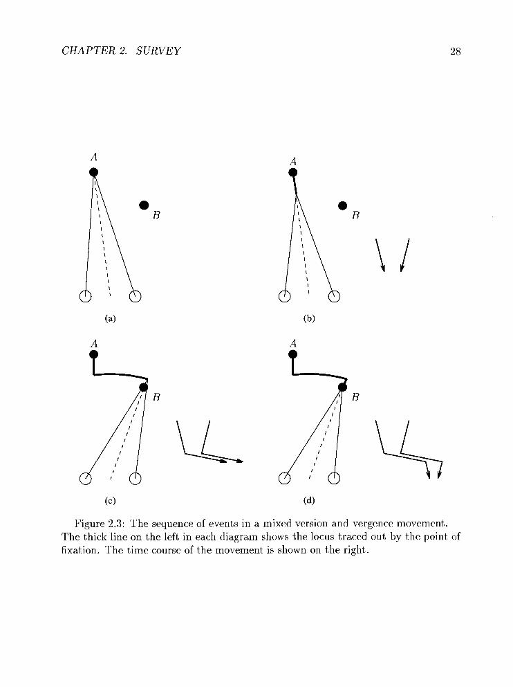
A similar pattern of eye movements is seen when a subject shifts his gaze from
one object to another [Yar57]. It starts with a slow symmetric vergence movement.
A conjunct saccadic version is then superimposed in the middle of the course to bring
the cyclopean axis in line with the target while the vergence movement is proceeding
to completion. The sequence is shown in Figure 2.3.
To effect good vision over the entire visual field, it is essential to be able to direct
the fovea at the objects of interest at various visual angles over the field. Gaze control,
which is manifested in various patterns of eye movements, is an area of research in
human perception. When a human subject is accomplishing a visual task, a scanpath

CHAPTER 2. SURVEY
Figure 2.2: The oculomotor map of visual space. The space coordinates are marked by lines of equal version (isophores) and lines of equal vergence (isotropes). The circular arcs are isophores and the rectangular hyperbolas are isotropes ([Car77, after [Lun48]]).
of eye fixations is normally observed to direct the gaze to a selection of objects in
the scene to collect the necessary visual information. Extensive research by Yarbus
[Yar67] demonstrates the goal-specific nature of scanpaths. In [NS7lb], Noton and
Stark postulated that memory of a pattern is formed in a sequence interleaved with
eye movements during the recognition process. Eye movement is also shown to be
critical for cognition. In Zinchenko and Vergiles's experiments [ZV72], subjects were
found to be unable to solve many of the visual problems if they were not allowed to
move their eyes.
In this thesis, a computational model for binocular fixation is investigated. It
leads to the development and implementation of a fixation model for space-variant
CHAPTER 2.
A
SURVEY
B
Figure 2.3: The sequence of events in a mixed version and vergence movement. The thick line on the left in each diagram shows the locus traced out by the point of fixation. The time course of the movement is shown on the right.
CHAPTER 2. SURVEY 29
sensing using RWT. A scanpath experiment, inspired by the eye movement research,
demonstrates the correct performance of our fixation system.
2.4 Advances in Stereo Verging Systems
In active visual following, the target is maintained at the center of the visual field,
i.e., its retinal slip is minimized. In their experiments with the Rochester head,
Coombs and Brown [CB92] studied the gaze holding problem in a dynamic environ-
ment. Binocular cue is used for vergence control. Once the cameras converge on the
target, the near-zero disparity filter can isolate the target's image from the other scene
objects. Smooth pursuit then keeps the target cent,ered by tracking the centroid of
the zero-disparity filtered window. Binocular disparity is used as a visual cue to ver-
gence error in the cameras' vergence control. Disparity is computed using the cepstral
filtering technique introduced in [BHT63]. A peak in the power cepstrum indicates
the disparity which is then converted to the vergence angle.
Gaze control comprises both gaze holding and shifting. In active stereo, fixation is
shifted from one point of attention to another. In our RWT fixation system, fixation is
carried out in the stages of peripheral vergence, saccadic version and foveal vergence.
This latter stage addresses the same issues as Coombs's vergence control. However,
a simple correlation on foveal features is shown to be sufficient in our case.
Stereo problems are greatly simplified in verging systems because vergence control
allows redistribution of the scene disparities around the fixation point, thus reducing
the disparities over an object of interest to near zero. Olson [Ols93] presented a simple
and fast stereo system that is suitable for the attentive processing of a fixated object.
In view of the narrow limits of the Panum's area, the fusible range is thought to be a

CHAPTER 2. SURVEY 3 0
privileged computational resource that provides good spatial information about the
fixation point. Assuming vergence control, Olson's stereo algorithm capitalizes on a
restricted disparity range. It gains from the slack demand for computation and allows
selective processing via disparity filtering. The disparities are examined in multiple
scales so that the system does not lose track of the rest of scene even though fixation
is attended to the target of interest.
The Panum's area in Olson's system [Ols93] is a fixed narrow band around the
~ i e t h - ~ i l e r circular horopter. Empirical data [Fis24, AOG321 indicate a spatially
varying Panum's area. Our RWT Panum's area resembles the empirically observed
one. The narrow Panum's region near the fovea is focused on the fixated target while
the deep Panum's area in periphery is attended to the rest of the scene.
Vergence is guided by stereo disparity. Stereo correspondence, paradoxically, is
difficult without fixation. An approach is to use other visual cues in cooperation with
stereo disparity in guiding the binocular vergence.
Pahlavan, Uhlin and Eklundh [PUE93] developed their machine fixation model af-
ter the fixational behaviors in human vision. The vergence component in their KTH
head-eye system is dealt with in accommodative and disparity aspects respectively.
The accommodative vergence is driven by focusing which is measured with the gray-
level variance. Correspondence is detected by calculating the normalized correlation
on the centrally symmetric positions between the left and right images. The blur and
disparity stimuli are then integrated to realize a cooperative effect on both accom-
modation and vergence of their KTH head. Incorporated with a stabilizing process
with symmetric version movement, the vergence system was demonstrated with an
experiment of real-time dynamic tracking of a moving person.

CHAPTER 2. SURVEY 31
Krotkov and Bajcsy [Kro89, KB931 developed and implemented the idea of co-
operative ranging in their agile stereo camera system [KSF88]. Accommodation and
vergence alone are weak depth cues [Gra65, GogGl]. Krotkov's system demonstrates
the reliability in ranging upon fusion of the focusing and stereo vergence components.
Initially, a focusing procedure computes the gross depth of the target scene feature
from the master camera. Based on that result, the vergence angle is calculated to
servo the fixation of both cameras on the target. Then execution is split into two
paths. One path performs stereo ranging with verification by focusing. The other
performs focus ranging. The operating windows on both cameras are related by
the disparity predicted from the focused depth. Improved reliability is successfully
demonstrated by sensor fusion at the level of data acquisition. This form of cooper-
ation exhibits visual behaviors analogous to human accommodative-convergence and
convergence-accommodation at various steps.
Grimson at al. [GLROK94] used color in cooperation with stereo cues. In their
work, they demonstrated how focus of attention is used to support the high level
task of efficient object recognition. Color is used for fast indexing to the region of
interest. Its use is combined with stereo cues to yield the disparity of the selected
region. By converging the cameras accordingly, attention is directed to it . A second
stereo matching within a narrow disparity range completes the figurelground seg-
mentation to un-clutter the scene for object recognition. The rationale is that both
correspondence and model matching would be significantly impeded if the scene were
cluttered.
Abbott and Ahuja [AA93] took integration of visual cues to great length in their
University of Illinois Active Vision System. Complementary strengths of different
cues are exploited in integration via active control of camera focus and orientation,

CHAPTER 2. SURVEY 3 2
as well as aperture and zoom settings, thus coupling image acquisition and surface
estimation dynamically and cooperatively in an active system. The idea agrees with
the active approach of intelligent data acquisition [Baj85]. Two phases are involved in
the process, namely fixation selection and surface reconstruction. Fixation selection
is posed as an optimization problem that seeks to minimize large camera movements
and develop the surface description outward from the current fixation, favoring the
unexplored area. Based on Sperling's energy model [Spe'iO], the surface reconstruction
is formulated to optimize among different cues of focus, disparity, surface smoothness.
The objective function also includes the image contrast and disagreement among the
cues and fixations. By selecting fixations to extend smoothly the evolving surface
map, their implementation produces dense depth information for a deep and wide
visual field.
Our active stereo ranging also employs the idea of active, intelligent data acquisi-
tion. Fixation favors conspicuous objects in the periphery. The range information is
evolved to more accurate levels from different fixations.
2.5 Non-frontal Imaging
In our binocular verging system, the RWT cameras represent a non-frontal imaging
device since the sensor surface is not assumed to be in a conventional frontal orienta-
tion. In our camera for imaging the road scene in a vehicle navigation problem [TL93],
a horizontal sensor plane offers the RWT a spatially varying resolution that offsets the
perspective distortion. This thesis will present a more elaborate non-frontal camera
model for RWT space-variant imaging in Chapter 4.
Although not aimed to achieve space-variant sensing, Krishnan and Ahuja [KA94]

CHAPTER 2. SURVEY 3 3
developed a non-frontal camera model for ranging using focusing. The non-frontal
imaging geometry is exploited in the way that varying image distance from the optical
center to the sensor plane occurs at different viewing angles. When the camera is
panned across the scene, an object will be imaged at different angles. At one of these
viewing angles during the course of panning, the image distance will be just right to
produce a sharp and focused image of the object.
In Krishnan and Ahuja's camera, the sensor plane is equipped with three degrees of
freedom. It can be translated, and rotated in two axes. Making use of the positioning
and orientation of the sensor plane, up to three object points in the scene can be
focused simultaneously. When the camera is swept across the scene, a series of images
are generated. Each point in the scene will be imaged in focus at one instance or
another. Therefore, the image series can then be analyzed to determine the sharply
focused regions, the union of which will produce a composite focused image of the
scene in a wide and deep field.
The camera can be used to obtain range from focusing as well. When the focus
criterion function (such as [Kro89, LG821) reaches its maximum for a scene point,
the parameters such as the pan angle, the objective lens' focal length and the sen-
sor's position and orientation are used to determine thk range value using the range
from focus methods [Pen87, EL93, KA931. Problems of variation in the registered
brightness and perspective warping are corrected at different imaging positions.
2.6 Directions in Active Vision Research
The National Science Foundation Active Vision Workshop held in 1991 set out the
directions in active vision research [SS91]. The attendees laid down five major research
CHAPTER2. SURVEY 34
areas include attention, foveate sensing, gaze control, eye-hand coordination, and
integration of vision with robot architectures.
This research fits in the picture because the RWT developed here provides a model
for foveate sensing. Motion stereo is studied in this sensing model and the fixation
mechanism for an RWT binocular system is presented. The system is suitable for
research into scanpath behaviors in attentive processing. It also promises applications
in vision-based tasks for situated robots.
Chapter 3
Reciprocal- Wedge Transform
3.1 The Mathematical Model
The Reciprocal-Wedge transform (RWT) was proposed as an alternative model for
space-variant sensing [TL93]. The RWT maps a rectangular image into a wedge-
shaped image. Spatially varying resolution is achieved as the smaller end of the
wedge is sampled with fewer pixels than the wider end is. Mathematically, the RWT
is defined as a mapping of the image pixels from the x-y space to a new u-v space
such that
U = 1/x , v = y/x . (3.1)
The lady's image in Figure 3.1 is used to illustrate how the Cartesian coordinates
are mapped back and forth1 to the RWT domain. The transformed image in Figure
3.l(b) shows a wedge-shape in an inside-out fashion because of the scaling effect of
the x reciprocal. Note the blurring at the periphery of Figure 3.1(c). In Figure
'Singularity occurs in the transform at x = 0 (the center strip). A variant of the RWT, which will be discussed in Section 3.1.2, was used in Figure 3.1 to cover the whole image including the center region.
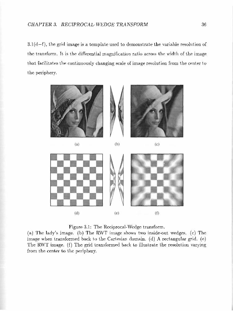
CHAPTER 3. RECIPROCAL-WEDGE TRANSFORM 36
3.l(d-f), the grid image is a template used to demonstrate the variable resolution of
the transform. It is the differential magnification ratio across the width of the image
that facilitates the continuously changing scale of image resolution from the center to
the periphery.
Figure 3.1: The Reciprocal-Wedge transform. (a) The lady's image. (b) The RWT image shows two inside-out wedges. (c) The image when transformed back to the Cartesian domain. (d) A rectangular grid. (e) The RWT image. (f) The grid transformed back to illustrate the resolution varying from the center to the periphery.
CHAPTER 3. RECIPROCAL- WEDGE TRANSFORM
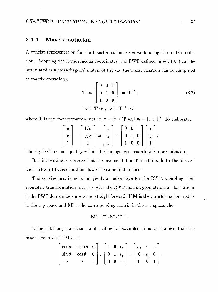
3.1.1 Matrix notation
A concise representation for the transformation is derivable using the matrix nota-
tion. Adopting the homogeneous coordinates, the RWT defined in eq. (3.1) can be
formulated as a cross-diagonal matrix of l's, and the transformation can be computed
as matrix operations.
where T is the transformation matrix, z = [x y lIt and w = [u v lIt. To elaborate,
The sign "E" means equality within the homogeneous coordinate representation.
It is interesting to observe that the inverse of T is T itself, i.e., both the forward
and backward transformations have the same matrix form.
The concise matrix notation yields an advantage for the RWT. Coupling their
geometric transformation matrices with the RWT matrix, geometric transformations
in the RWT domain become rather straightforward. If M is the transformation matrix
in the x-y space and M' is the corresponding matrix in the u-v space, then
Using rotation, translation and scaling as examples, it is well-known that the
respective matrices M are:

CHAPTER 3. RECIPROCAL- WEDGE TRANSFORM 38
Since both T and T-' are cross-diagonal matrices of 1's (eq. (3.2)), their effect on
M involves only row and column interchange. Thus, the respective matrices for the
RWT domain can easily be derived as:
0 1 0 0 1 0 0 [ t coso si:o], I t g 1 o ] , l o sy 0 1 ,
0 -sin 0 cos 0 t , 0 1 0 0 s,
Figure 3.2 shows the direct application of the transformation matrices in the RWT
domain. In Figure 3.2(a), the matrices are applied directly in the u-v space. For visual
apprehension, the x-y representation of the transformed results is reconstructed in
Figure 3.2(b) to demonstrate the effects of the three matrices.
3.1.2 Remedy to singularity
The singularity of the RWT exists at x = 0, i.e., u = 110 = cc and v = y/O. Two
remedies to the problem are proposed: patching and shifting.
Assuming the origin of the x-y space is at the center of the image, the patching
method provides an expedient fix to the singularity problem. The method excludes
a strip of width 26 at the center, where x value is zero or near zero, from the range
of the RWT. The center strip from the original uniform-resolution image is then used
to patch up the two wedge images from the RWT.2 It is convenient in many cases
to use a uniform-resolution model for the fovea because it is essential to maintain a
high acuity within the extent of the fovea for most visual behaviors. Besides, the rich
repertoire of existing computer vision techniques could be used for foveal processing.
The shifting method is an alternative way of fixing the singularity problem. It
is to introduce a shift parameter a in the RWT.3 This variant formulation is called
'The log-polar transform also has the singularity problem at r = 0. A uniform-resolution patch at the center of the image is constructed in the prototype camera [VdSKC+89, KVdS+SO].
3A similar shift parameter is also used in log-polar transform to the same effect [Sch80, RS901.

CHAPTER 3. RECIPROCAL- WEDGE TRANSFORM 39
Figure 3.2: Geometric transformations on u-v images. (a) Direct application of the scaling, rotational and translational transformations on the u-v lady's image. (b) The x-y representation of the transformation results are reconstructed for visual apprehension of the effects of the scaling, rotation and translation.
Shifted Reciprocal- Wedge Transform (S-RWT)4 [TL93].
Both the forward and backward transformations for the S-RWT remain the same
cross-diagonal matrix (eq. (3.2)) except the additional parameter a.
41n fact, S-RWT has been used for the transformation in Figure 3.1 to take care of the singularity inherent in the original RWT equations (eq. (3.1))

CHAPTER 3. RECIPROCAL- WZDGE TRANSFORM 40
The effect of the parameter a is to horizontally shift the center strip (and the
rest of the image) away from x = 0, or equivalently, shift the x axis in the Cartesian
image. The parameter a should be of opposite sign for the left and right halves of the
Cartesian image, i.e., the two halves of the image are respectively shifted in opposite
directions. There is an advantage with the inclusion of the shift parameter in the S-
RWT. As the space-variant resolution in RWT is caused by the x-reciprocal function
(eq. (3.1)), the use of a on x in eq. (3.3) allows adjustment on the speed of changing
scale of the resolution from fovea to periphery. Meanwhile, since a leads only to a
horizontal shift in the Cartesian image, for simplicity we can still use eq. (3.1) for the
RWT for analysis of its properties.
It is not difficult to see that a combination of both patching and shifting can be
adopted to take advantage of both techniques. Each of the single techniques can then
be viewed as a special case where either S = 0 or a = 0. Our camera design in Section
4.4.2 will readily accommodate all these choices.
3.1.3 The RWT View-of- World
We now examine the effects of the forward and backward RWT. (The patching method
is used for illustration in Figure 3.3. The S-RWT or the combination of the patching
and shifting methods would yield similar results.)
Figure 3.3(a) depicts the effect of the forward RWT (T). Excluding the strip of
width 6, one half of the rectangular x-y image is turned into a wedge in an inside-
out fashion because of the scaling effect of the x reciprocal. Figure 3.3(b) shows the
reassembled version which comprises the two halves of the RWT image and the center
patch for the purpose of visual apprehension. The reassembled version is also referred
as the bipolar representation of the RWT image because the origins for the left and
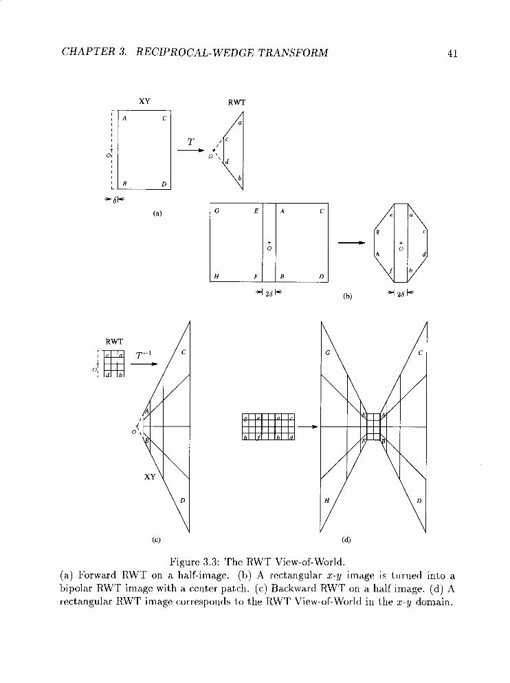
CHAPTER 3. RECIPROCAL-WEDGE TRANSFORM
XY
01 !'E 46k
(4
RWT
RWT
Figure 3.3: The RWT View-of-World. -
(a) Forward RWT on a half-image. (b) A rectangular x-y image is turned into a bipolar RWT image with a center patch. (c) Backward RWT on a half-image. (d) A rectangular RWT image corresponds to the RWT View-of-World in the x-y domain.

CHAPTER 3. RECIPROCAL- WEDGE TRANSFORM 42
right half-spaces are independently flipped to the two antipodes. As shown, the two
pieces of the wedges have been properly flipped before the merging.
Figure 3.3(c) depicts the backward RWT (T-I). Since T = T-l, Figure 3.3(c) and
3.3(a) appear similar, except that the RWT images in both cases are much smaller
because of the data reduction. Nevertheless, Figure 3.3(c) reveals that an RWT
rectangular region corresponds to a wedge-shape area in the x-y space. Figure 3.3(d)
shows the complete mapping including the center patch, the resulting image in the
x-y space is the RWT View-of- World (VOW). The RWT-VOW is the effective space-
variant view from a RWT camera using square/rectangular sensing elements. The
center part (fovea) of the VOW obtains the highest resolution, which drops rapidly
towards both sides (periphery).
Figure 3.4 illustrates how images in the Cartesian coordinates are mapped to the
RWT domain, and then mapped back. The lady's image in Figure 3.4(a) is the
original image (resolution 400 x 200) in the x-y space. The combination method is
applied where S = 5 and a = 30. The transformed image in Figure 3.4(b) shows the
two wedges. The image is reduced to approximately 10% of its original size. Figure
3.4(c) shows the bipolar representation of the RWT image. Note the nice feature that
the bipolar image is continuous at the two borders of the patch. Figure 3.4(d) is the
restored lady's image. The blurring at the periphery is due to the inevitable (and
desirable) loss of details after the image was reduced by the RWT.
In Figure 3.4, a grid image is also provided to clearly demonstrate the extent of the
spatially varying resolution produced by the transformation. A continuously changing
scale of resolution from the center to the periphery across the width of the image is
supported.
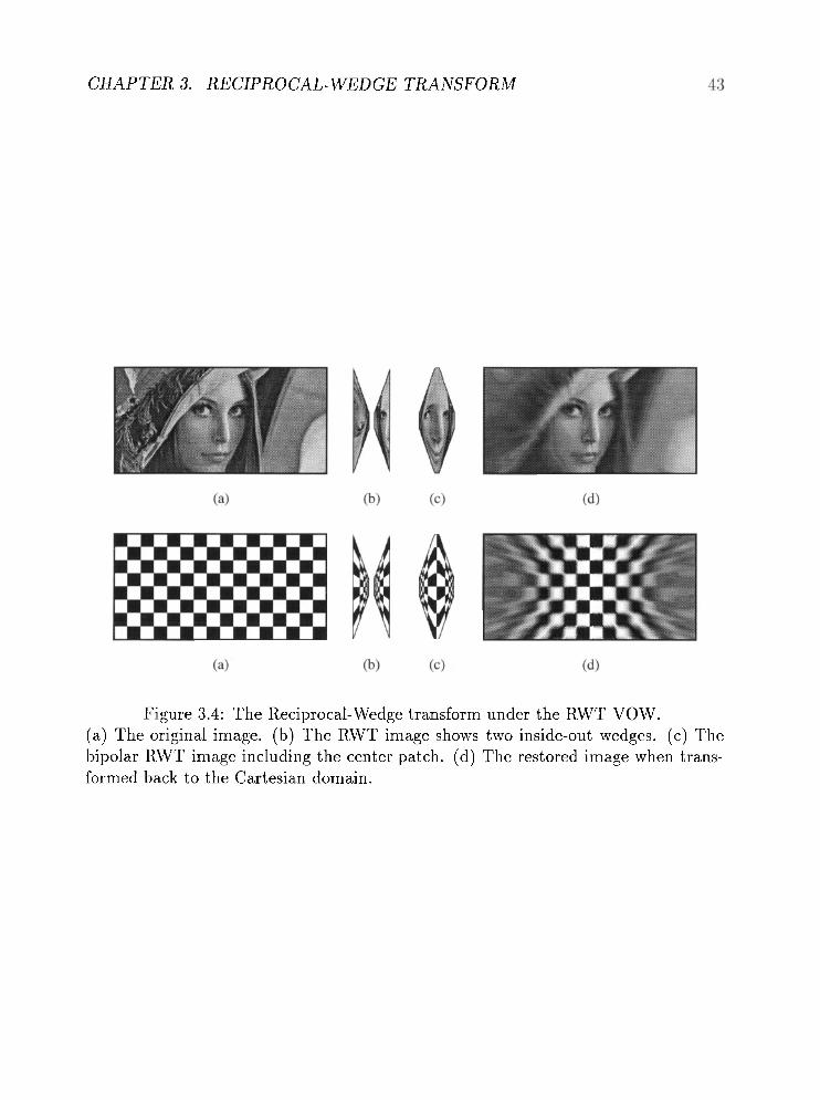
CHAPTER 3. RECIPROCAL- WEDGE TRANSFORM
Figure 3.4: The Reciprocal-Wedge transform under the RWT VOW. (a) The original image. (b) The RWT image shows two inside-out wedges. (c) The bipolar RWT image including the center patch. (d) The restored image when trans- I formed back to the Cartesian domain.

CHAPTER 3. RECIPROCAL- WEDGE TRANSFORM
3.2 Transformation on Linear Structures
Exploiting the polar coordinate representation, the log-polar transform gracefully sim-
plifies the computation of centric transformations. Rotation and scaling about the
origin become operations along the log r and 8 axes. However, the polar coordinate
representation adversely obscures other geometric patterns. For instance, linear struc-
tures get mapped to complicated patterns of logarithmic sine curves. Since both linear
features and translations are very common in image analysis, this seems to be a major
drawback of the log-polar transform.
RWT, on the contrary, does not employ the polar coordinates. It does not perform
as well in computation of centric transformations. However, linearity of lines in the x-
y domain is preserved over the transformation. Furthermore, we argue that the RWT
does not complicate curves in general. If a curve is represented with a polynomial,
the degree does not change after the transformation.
3.2.1 Preservation of linear features
Lines exhibit interesting properties in the RWT. In fact, the following transformation
dual (L,, and L,,) of a line can be derived:
Given L,,, the equation for L,, is readily obtained by substituting x and y in L,,
with llu and vlu respectively. It is obvious that the transformed structure L,, is also
a line, which implies that the linearity of the line is preserved.5 It is interesting to
note that the values for the slope and intercept are interchanged between the trans-
formation dual. Inferring from that, parallel lines with the same slope in x-y will be
5Linear features are also preserved in the S-RWT. A line LZy : y = m + c is mapped to a line L,, : v = ( c - ma)u + m.
CHAPTER 3. RECIPROCAL- WEDGE TRANSFORM 4 5
mapped to u-v lines concurrent at the same v-intercept. Inversely, lines concurrent at
the same y-intercept will form parallel lines in the u-v domain.
Extension to curves. Let a curve in x-y be denoted as:
By substituting l / u for x and v/u for y, and rewriting the indices, the polynomial in
u-v becomes: n n-i
i = O j = O
This shows that the degree of the polynomial is preserved over the transformation.
The shape of the curve may be different in the transform domain as the coefficients
have been interchanged. For instance, a circle in x-y would be mapped to an ellipse
in u-v. (It would be a hyperbola or parabola should the circle be transversed by
the y-axis.) The significance is that the RWT does not complicate curve patterns.
In comparison, after the log-polar mapping, the resulting curve no longer keeps its
polynomial form. One disadvantage is that undesirable complexity is introduced when
problems of shape analysis or image data modeling are dealt with.
3.2.2 Line detection using the Hough transform
The Hough transform [DH72] provides a powerful tool for feature detection. The
technique is most effective for line detection [TL92]. The preservation of the linearity
of lines over the RWT implies that line detection using the Hough transform would
be as simple in the RWT as in the Cartesian domain. With the switching between
the slope and intercept parameters (eq. (3.4)), the vote patterns in the Hough space
for the Cartesian and the RWT images form an interesting dual of reflection about
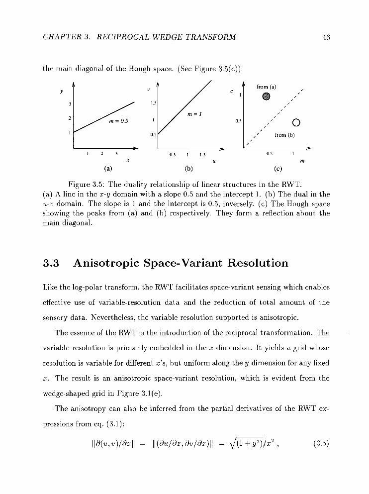
CHAPTER 3. RECIPROCAL- WEDGE TRANSFORM
the main diagonal of the Hough space. (See Figure 3.5(c)).
Figure 3.5: The duality relationship of linear structures in the RWT. (a) A line in the x-y domain with a slope 0.5 and the intercept 1. (b) The dual in the u-v domain. The slope is 1 and the intercept is 0.5, inversely. (c) The Hough space showing the peaks from (a) and (b) respectively. They form a reflection about the main diagonal.
3.3 Anisotropic Space-Variant Resolution
Like the log-polar transform, the RWT facilitates space-variant sensing which enables
effective use of variable-resolution data and the reduction of total amount of the
sensory data. Nevertheless, the variable resolution supported is anisotropic.
The essence of the RWT is the introduction of the reciprocal transformation. The
variable resolution is primarily embedded in the x dimension. It yields a grid whose
resolution is variable for different x's, but uniform along the y dimension for any fixed
x. The result is an anisotropic space-variant resolution, which is evident from the
wedge-shaped grid in Figure 3.1 (e).
The anisotropy can also
pressions from eq. (3.1):
IP(% v)laxll
be inferred from the partial derivatives of the RWT ex-

CHAPTER 3. RECIPROCAL- WEDGE TRANSFORM 4 7
where )I.II denotes the vector norm. Eqs. (3.5) and (3.6) show that the pixel resolution
does not vary in the same manner for different directions. The grid width in the x
direction (for a fixed y) is mapped to a size diminishing in reciprocal of x2. In the y
direction, the grid height is mapped by a function of 1/x to a uniform size independent
of the y value. Furthermore,
Hence, the absolute value of the above Jacobian determinant is
which indicates that the area of a pixel is reduced by a factor of l / x 3 after the RWT.
On the contrary, the log-polar transform provides an isotropic variable resolution.
The grid when mapped to the log-polar image changes size in the same scale in
all directions. Sampling along the radial direction, the rate of change of the pixel
resolution is
Ildwldrll = Id(logr)/drl = l / r
The area of a pixel thus diminishes isotropically in the rate of l / r 2 .
The log-polar transform benefits from its conformal mapping. As the differential
and local operators have valid conformal transplants in the log-polar domain, the
related image processing tools and vision algorithms can also be available for pro-
cessing in the log-polar domain with minimum overhead [WC79]. Compared to the
log-polar, the RWT is neither conformal nor isotropic. The RWT, however, can also
benefits from its matrix representation. Its matrices facilitate convenient mapping
of linear transformations from the Cartesian to the RWT coordinates. As a result,

CHAPTER 3. RECIPROCAL- WEDGE TRANSFORM
the established linear transformations for the Cartesian image processing are readily
applicable in the RWT as well. (The application of geometric transformations on the
RWT images has been demonstrated in Section 3.1.1.)
In the log-polar, the isotropic mapping facilitates the form invariance properties
for centric patterns. In the RWT, it is the anisotropic mapping that enables the
directionally biased RWT variable resolution. The directional variable resolution does
not only benefit linear feature processing, but is also generally suitable for problems
of translational in nature, such as motion stereo and binocular disparity computation.
Hence, the anisotropic mapping of the RWT makes it distinguished from the log-
polar transform. On one hand, it is comparable to the log-polar for its space-variant
resolution and data reduction. On the other hand, it is complementary to the log-polar
for its suitability for linear transformations, lines and translations.
3.4 Pyramidal Implementat ion
The capacity for parallel processing and versatility of multiple resolutions have made
the pyramidal architecture a widely adopted structure for fast image processing and
parallel modeling for various visual processes. The Image Understanding Architecture
[WB91] is an ambitious project on a three-dimensional pyramidal architecture. How-
ever, the two-dimensional pyramids have their advantages of cost-effectiveness and
flexibility. The SFU hybrid pyramid [ELT+92] is a heterogeneous system offering the
versatility in both iconic [LZ93] and functional [Li91] pyramidal mappings. In this
section, a pyramidal implementation on the SFU pyramid for fast generation of RWT
images is presented.
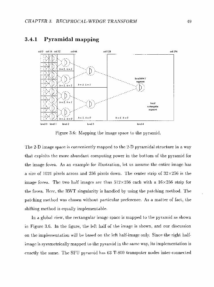
CHAPTER 3. RECIPROCAL- WEDGE TRANSFORM
3.4.1 Pyramidal mapping
col0 col 16 co132 co164 col 128
level 0 level 1 level 2 level 3 level 4
Figure 3.6: Mapping the image space to the pyramid.
The 2-D image space is conveniently mapped to the 2-D pyramidal structure in a way
that exploits the more abundant computing power in the bottom of the pyramid for
the image fovea. As an example for illustration, let us assume the entire image has
a size of 1024 pixels across and 256 pixels down. The center strip of 32x256 is the
image fovea. The two half images are thus 512x256 each with a 16x256 strip for
the fovea. Here, the RWT singularity is handled by using the patching method. The
patching method was chosen without particular preference. As a matter of fact, the
shifting method is equally implementable.
In a global view, the rectangular image space is mapped to the pyramid as shown
in Figure 3.6. In the figure, the left half of the image is shown, and our discussion
on the implementation will be based on the left half-image only. Since the right half-
image is symmetrically mapped to the pyramid in the same way, its implementation is
exactly the same. The SFU pyramid has 63 T-800 transputer nodes inter-connected

CHAPTER 3. RECIPROCAL- WEDGE TRANSFORM 50
in a binary tree. Together they form a two-dimensional pyramid of 6 levels. For
illustration, a simpler version of 5 levels are used in the explanation. The dotted
circles and arcs in Figure 3.6 are showing the 5 levels of the pyramid. The bottom
level is reserved for uniform-resolution processing for the image fovea. In the figure,
they are the level 0, and are not participating in the RWT image generation.
The pyramid nodes and their corresponding image blocks are labelled with the h
and k indices. The h index is related to the level number of the node, and the k index
is the node's position within the level. Refer to Figure 3.6 for the k ordering of the
nodes within different levels.
The pyramidal algorithm can be described in 2 steps. First, A pyramidal reduction
process transfers the image segments up the pyramid from the bottom level. At each
node, the image segment is reduced to half the resolution of the one from below. In
the second step, each node performs the transformation to obtained an RWT segment
for the local node. When the pyramid program is running, these 2 steps are actually
pipelined together.
3.4.2 Pyramidal reduction
The rectangular image is loaded onto the pyramid from the bottom level up. Our
mapping algorithm partitions the rectangular image space into segments of size of
two's powers, and distributes the segments to the pyramid nodes in the way depicted
in Figure 3.6. The segments, however, are stored in reduced resolution at each level.
When the image is first loaded onto the level 0 nodes, each of the nodes gets a ribbon
of 512 x 8. These foveal nodes then retain a block of 16 x 8 as the uniform-resolution
fovea. The rest of the ribbon is then passed to the parent at level 1.
From level 1 on, the nodes are in the variable resolution region. They are involved

CHAPTER 3. RECIPROCAL- WEDGE TRANSFORM 5 1
in the RWT image generation. Now, each level 1 node merges the 2 8-ribbons from its
children to generate a 16-ribbon. A 16x 16 block is retained as a local segment. This
segment will get mapped to the RWT image in the later step. The merge operation
can be formulated as follows:
A10i,j+16 if z < 8
Aooi-s,j+16 otherwise
where Ahi,j is the image segment at the level h, and A ~ ~ - ~ ~ , ~ is the kth child the level
h - 1. It is the right child when k = 0 and the left child when k = 1. Figure 3.7
presents a graphical description of this step. The segment of the level h node is a
merged version from both children at the level h - 1.
Figure 3.7: The pyramidal reduction step.
From level 2 on, every node takes 2 16-ribbons from its children, reduce-merges
them into a 16-ribbon at half resolution. Again, a 16x16 block is retained for the
local segment (Figure 3.7). The reduce-merge operation can be formulated as follows:
h ~ l ~ - ~ ~ ~ , ~ ~ + ~ ~ if i < 8 A ; . = J
A ~ ~ - ~ 2i-16,2j+16 otherwise
At the end of this image distribution phase, each node has a 16x 16 local segment
of the original image. These segments have different resolutions according to their
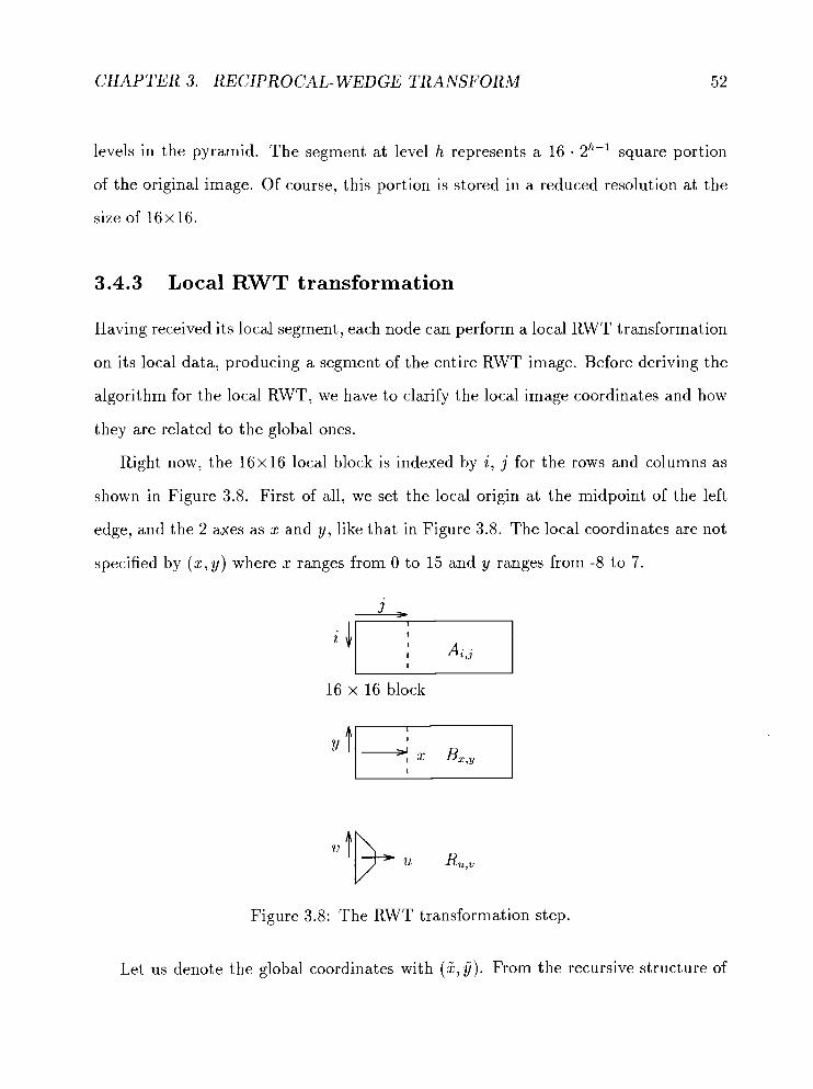
CHAPTER 3. RECIPROCAL- WEDGE TRANSFORM 52
levels in the pyramid. The segment at level h represents a 16 2h-1 square portion
of the original image. Of course, this portion is stored in a reduced resolution at the
size of 16x16.
3.4.3 Local RWT transformation
Having received its local segment, each node can perform a local RWT transformation
on its local data, producing a segment of the entire RWT image. Before deriving the
algorithm for the local RWT, we have to clarify the local image coordinates and how
they are related to the global ones.
Right now, the 1 6 x 1 6 local block is indexed by i, j for the rows and columns as
shown in Figure 3.8. First of all, we set the local origin at the midpoint of the left
edge, and the 2 axes as x and y, like that in Figure 3.8. The local coordinates are not
specified by (x, y) where x ranges from 0 to 15 and y ranges from -8 to 7.
J ,
i y - j - T J
16 x 16 block
Figure 3.8: The RWT transformation step.
Let us denote the global coordinates with ( 2 , y"). From the recursive structure of

CHAPTER 3. RECIPROCAL- WEDGE TRANSFORM 5 3
the pyramidal reduction, the local coordinates (x, y ) can be related to the global ( 2 , i j)
as follows:
where m is the height (maximum level) of the pyramid.
Let (u, v ) be the coordinates for the global RWT image. The global transformation
is (eq. (3.1)) 1 62 u = - 16. ij - , v = - . x x
Since it is desirable to have the resolution of the RWT image be continuous with the
foveal resolution at the boundary between the two, scale factors have been put in the
above equations to adjust the u-v resolution. By eqs. (3.8) and (3.9),
Alternatively, the global transformation in eqs. (3.10) and (3.11) can be performed
in 3 simple operations for easy implementation.
1 62 u=-
16 - y Local transform : v = ---
x + 1 6 ' x + 1 6 ' (2k - 2m-h + 1)
v shearing : 2 ' U ,
1 u scaling : -
2h-1 * (3.14)
Let A;,j be the local image segment, B,,, be the remapped image of Ai j with
the origin set to the center row and the y axis is upright. R,,, is the local RWT
segment. Figure 3.8 indicates the relationships among the 3 coordinate systems. By
eqs. (3.12-3.14), the transformation can be formulated as in the following 4 steps:

CHAPTER 3. RECIPROCAL- WEDGE TRANSFORM
1. Move the axes: B,,, =
2. Local transform: R,, = B g - IS,%
3. v-shear: RU,V = 8 ( ~ k - ' 2 m - ~ + l u,u- 2
4. u-scale: &,V = RP-~~,V
At the end, each node will have its local RWT segment as illustrated in Figure
3.6.

Chapter 4
Camera Model
4.1 The RWT Projective Model
Figure 3.l(b) appears like the view of a picture from a grazing angle. In fact, one
could regard the RWT as a projection of an image on a plane perpendicular to it.
Examine the perspective projection in which the three-dimensional X Y Z space is
projected onto the two-dimensional 2 - Y plane at X = 1 (Figure 4.1). Let the three-
dimensional point be (X, Y, 2) and the projection be (Z', Y').
Now, the equations in (3.1) can be made equivalent to those in eq. (4.1) if the
terms x, y , 1, u , v in (3.1) are unified with the X , Y, Z, Z', Y' in (4.1), respectively.
In that sense, the RWT described by eq. (3.1) can also be viewed as a perspective
reprojection in which the original image is on the X-Y plane at Z = 1, and it is
projected onto the 2 -Y plane at X = 1.'
'For simplicity, both focal lengths have been chosen as 1 in the above discussion. In general, the two images planes are at Z = f and X = f'. As a result, the projective model will yield u = l / x . f . f' and u = ylx . f', which differ from eq. (3.1) by constant factors.

CHAPTER 4. CAMERA MODEL
original P2
image - \ I \ \
center of projection
plane
Figure 4.1: A perspective projection model. The original image is placed on the X-Y plane at Z = 1. It is reprojected onto the 2-Y projection plane at X = 1. The pixels pl and p2 are projected to pi and p',, respectively.
It is interesting to notice that potentially the RWT could be implemented in
hardware. Since the RWT image can be considered as another perspective projection
of the Cartesian image onto an orthogonal projection plane, in a simplistic point of
view, we can cascade the two processes into one. Figure 4.2 illustrates the idea. The
sensor is fitted directly on the RWT projection plane mounted sideways. Thereby,
the rays from the imaged objects strike directly onto the RWT sensor plane. The
sensor plane is installed in two half-planes, the left and right ones, respectively, for
the convenience of taking care of objects on each side of the optical axis.
The RWT camera can use a uniform sensor, which is cheap to fabricate. Space-
variant sensing is realized by the oblique perspective projection on the sensor plane.
The same sensor area on the plane yields variable area coverage of the visual field
depending on the angle of projection. As shown in Figure 3.3, rectangular x-y images
are turned into wedge-shaped RWT images. A rectangular RWT sensor array inversely
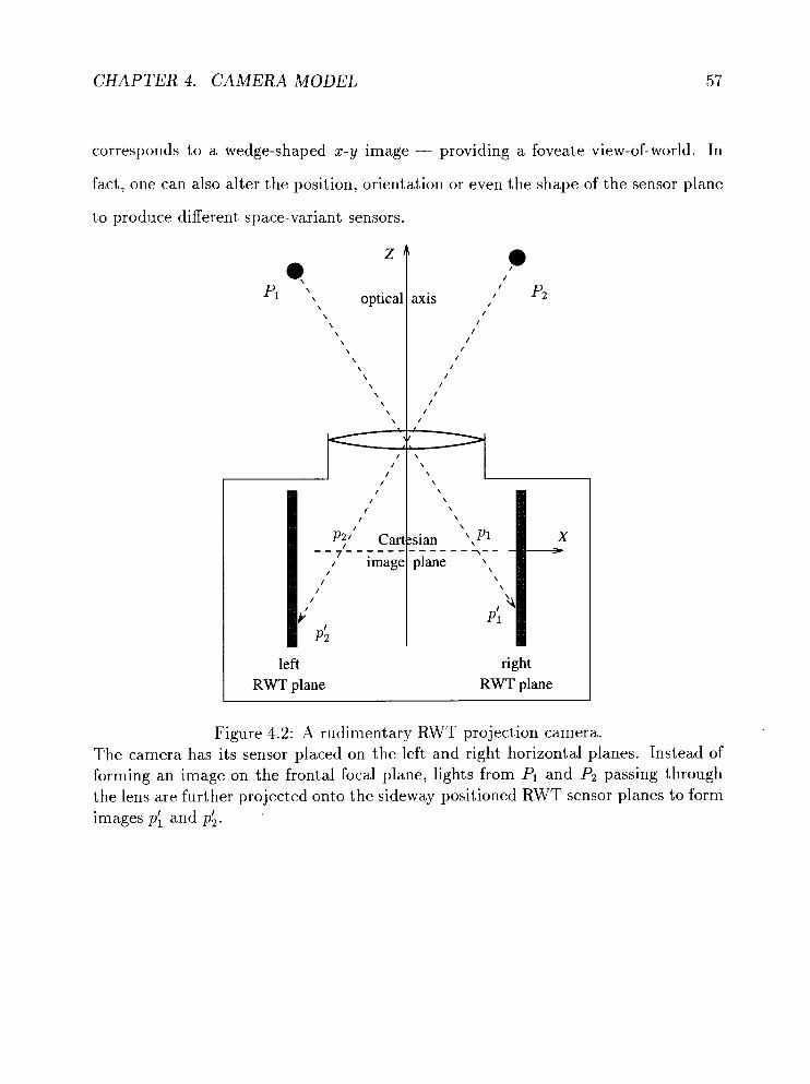
C H A P T E R 4. C A M E R A MODEL 5 7
corresponds to a wedge-shaped x-y image - providing a foveate view-of-world. In
fact, one can also alter the position, orientation or even the shape of the sensor plane
to produce different space-variant sensors.
PI \ \ optical \
left
-
RWT plane right
RWT plane
Figure 4.2: A rudimentary RWT projection camera. The camera has its sensor placed on the left and right horizontal planes. Instead of forming an image on the frontal focal plane, lights from PI and P2 passing through the lens are further projected onto the sideway-positioned RWT sensor planes to form images pl and p i .

CHAPTER 4. C A M E R A MODEL
4.2 Non-Paraxial Focusing
The above discussion delineates a rudimentary idea of the RWT camera design. A
prominent problem of Figure 4.2 is the necessity of focusing on a deep image plane in
parallel to the optical axis. As shown in Figure 4.3 the object forms a sharp image
on the focal plane normal to the optical axis. However, upon further projection onto
the RWT plane which is positioned sideways and off-axis, the rays diverge, casting a
blurred image on the RWT plane.
Figure 4. 3: The focusing problem c
sharp blurred image image
RWT image plane
)f the sideway-positioned RWT projection plane.
In general, it is difficult to get a focused image on an off-axis plane. Ordinary
cameras have paraxial focal planes, i.e., only objects that are near the optical axis
will form focused images on the focal plane. The pair of object and image points are
called conjugate points and the planes through these points are the conjugate planes.
This is true only under paraxial conditions. However, the RWT image plane in Figure
4.3 is located off-axis, and the condition for lens focusing is not paraxial.

CHAPTER 4. C A M E R A MODEL
4.2.1 The RWT lens
In addition to its off-axis position, the RWT image plane also assumes a non-frontal
orientation like the one in the Krishnan's camera [KA94]. An optical condition of such
non-frontal projection is known as the Sheimpflug condition [Bro65]. It occurs between
tilted object and image planes (as shown in Figure 4.4). In fact, the projective model
of the RWT can be achieved as non-frontal focusing between orthogonal conjugate
planes.
Consider an image plane oriented at an angle to the optical axis of a lens. Without
loss of generality, the problem is dealt with in the 2-D 2 - X plane. The result can
be readily extended to the 3-D X Y Z space. Let the optical axis be aligned with the
Z axis, and the lens be on the X axis. The normal of the image plane is on the
2-X plane. The resulting configuration is as shown in Figure 4.4. A point on the
image plane is denoted as PI(ZI, XI), and its conjugate object point is Po(Zo, Xo).
In the 2-D Z-X space, the image plane is a line. Let us denote it with the equation
XI = m ~ . ZI + CI, where r n ~ and CI are the slope and X-intercept of the line. As Po
and PI are related by the lens refraction formula and are collinear along the principal
ray which travels through the optical center of the lens, the conjugate relationship
between the object and image plane can be derived by solving the equations involving
the lens formula, the ~rincipal ray geometry and the plane equation.
1 1 1 Lens formula : - -+ -= -
20 21 f '
Principal ray : x o XI
- z o 21'
Image plane : XI = r n ~ . 21 + C I
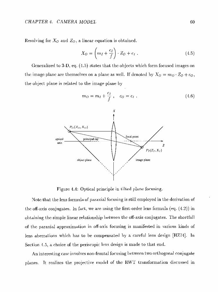
CHAPTER 4. CAMERA MODEL
Resolving for Xo and Zo, a linear equation is obtained.
Generalized to 3-D, eq. (4.5) states that the objects which form focused images on
the image plane are themselves on a plane as well. If denoted by Xo = m o . Zo + co,
the object plane is related to the image plane by
optical D
axis Z
object plane \ v \ image plane
Figure 4.4: Optical principle in tilted plane focusing.
Note that the lens formula of paraxial focusing is still employed in the derivation of
the off-axis conjugates. In fact, we are using the first-order lens formula (eq. (4.2)) in
obtaining the simple linear relationship between the off-axis conjugates. The shortfall
of the paraxial approximation in off-axis focusing is manifested in various kinds of
lens aberrations which has to be compensated by a careful lens design [HZ74]. In
Section 4.5, a choice of the periscopic lens design is made to that end.
An interesting case involves non-frontal focusing between two orthogonal conjugate
planes. It realizes the projective model of the RWT transformation discussed in

CHAPTER 4. CAMERA MODEL 6 1
Section 4.1, and successfully overcomes the focusing problem which would render
the simple camera model in Figure 4.2 impractical. In the new camera model, the
orthogonal conjugate planes are realized with a lens system constructed as in Figure
4.4. Both the object and image planes are at 45' to the X axis. If -mo = m~ =
tan 45" = 1, from eq. (4.6),
It means that the planes are installed at 90' to each other. They are arranged sym-
metrically on both sides of the lens. For the lens having a focal length f , the planes
intersect at 2 f below the lens.
The lens is re-drawn in Figure 4.5. Herein, the lens system is rotated by 45" to
ease the distance computation for the next step. Now, the object plane is the vertical
plane and the image plane is the horizontal one. The lens is located at the origin of
the X Y Z coordinate space. For simplicity, the normal distance of the planes to the
lens is again assigned a unit value. This makes the lens parameters consistent with
the projective model in Figure 4.1, thus realizing the RWT transformation as defined
in eq. (3.1). If the normal distance is not equal to one, then all the other distance
measurements will simply be scaled by constant factors, as explained in Section 4.1.
From the geometry, 0F0 is (Xo, Yo, 1), and O ~ O is collinear with 0?1. Therefore,
This can be denoted as:
which illustrates that such an projection between orthogonal planes through the origin
achieves the RWT transformation.

CHAPTER 4. CAMERA MODEL
object I\,
Figure 4.5: The prototype RWT lens. The object and image planes are at 45' symmetrically on both sides of the lens. The normal distance of the planes from the lens is assigned a unit value. The principal ray from Po, traveling through the optical center 0 to PI is shown.
4.3 Projecting the Singularity
Similar to the singularity problem at x = 0 in eq. (3.1), the projective model from
Figure 4.2 also fails for points near the Z axis. In this section, the patching and
shifting methods discussed in Section 3.1.2 are employed as the practical fix in the
design for the camera. The following proposes three techniques, namely the U-plane
projection, the V-plane projection and the displaced-center projection. The U-plane
projection implements the patching method whereas the latter two provide alternative
techniques for implementing the shifting method.
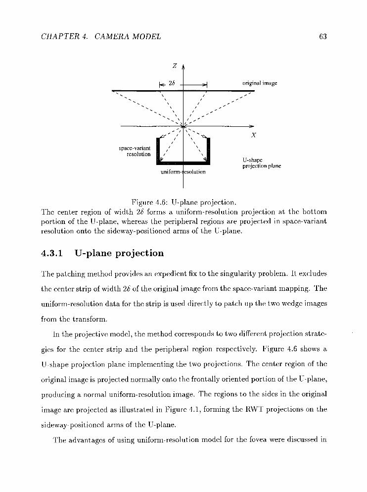
CHAPTER 4. CAMERA MODEL
b 2a t 4 original image
X
space-variant resolution
U-shape proiection plane
1 A -
uniform- esolution
Figure 4.6: U-plane projection. The center region of width 26 forms a uniform-resolution projection at the bottom portion of the U-plane, whereas the peripheral regions are projected in space-variant resolution onto the sideway-positioned arms of the U-plane.
4.3.1 U-plane projection
The patching method provides an expedient fix to the singularity problem. It excludes
the center strip of width 26 of the original image from the space-variant mapping. The
uniform-resolution data for the strip is used directly to patch up the two wedge images
from the transform.
In the projective model, the method corresponds to two different projection strate-
gies for the center strip and the peripheral region respectively. Figure 4.6 shows a
U-shape projection plane implementing the two projections. The center region of the
original image is projected normally onto the frontally oriented portion of the U-plane,
producing a normal uniform-resolution image. The regions to the sides in the original
image are projected as illustrated in Figure 4.1, forming the RWT projections on the
sideway-positioned arms of the U-plane.
The advantages of using uniform-resolution model for the fovea were discussed in

C H A P T E R 4. C A M E R A MODEL 64
Section 3.1.2. In fact, the U-plane model supports a seamless joint between the central
rectangular fovea and the peripheral wedge-shaped regions. On the contrary, the
spatially uninterrupted connection between the fovea and periphery is not supported
in the log-polar implementation [VdSKC+89]. The square grid for the fovea and the
ring structures for the log-polar periphery cannot simply be patched together.
4.3.2 V-plane projection
The shifting method discussed in Section 3.1.2 has been formulated in eq. (3.3) as
the S-RWT. The following shows that the S-RWT can also be implemented with a
V-plane projection.
Figure 4.7 depicts the V-plane projection. The two projection planes in Figure
4.2 are joined to form a V in this figure. The left arm of the V forms the projec-
tion plane for the right half of the original image and the right arm of the V is the
projection plane for the left half. The singularity problem disappears because the
center region of the original image gets projected to a u position on the V-plane. It
can be observed that the orientation of the V arms is not as steep as that of the
sideway-positioned projection plane in Figure 4.1. A less drastic space-variant reso-
lution should be expected. In fact, it can be shown that such a V-plane projection
implements the space-variant resolution of the S-RWT of eq. (3.3).
Since the projection occurs independently on each side of the image, without loss
of generality we examine the projection from the right side of the original image onto
the left arm of the V. Figure 4.8 shows the ray diagram of the projection. A point
P on the original image is projected to Q on the projection plane. 0 is the center
of projection, and E is the origin of the x-y space. To be consistent with the S-
RWT formulation in eq. (3.3), the origin of the u-v space F is defined as the point of

C H A P T E R 4. C A M E R A MODEL
I original image
projection plane
Figure 4.7: V-plane projection. The left arm of the V forms the projection plane for the right half of the original image and the right arm of the V is for the left half. The singularity problem is resolved, and space-variant resolution is effected on both projection planes.
projection when x = oo and y = 0.
From the geometry in Figure 4.8, LPRO = LROF = 0.
- - r OF = RF = ---
2 cos 0 , - RE = rcos0 .
From the similar triangles, - - R E + x OF
Using (4.9) and (4.10) in (4.11),
by letting f = r l ( 2 cos O ) , and a = r cos 0 - r l ( 2 cos 6 ) .
Imagine the vertical dimension inlout of the paper. It defines the y coordinates
on the image plane and the v coordinates on the projection plane. Again, from the

CHAPTER 4. CAMERA MODEL
original image x = o E x P
Figure 4.8: Geometry of the V-projection from P to Q.
similar triangles,
Combining (4.13) and (4.14),
From (4.12) and (4.15), we conclude that the u and v coordinates from the V-
plane projection are effectively computing the S-RWT as defined in eq. (3.3) within
a constant factor f .
4.3.3 Displaced-center project ion
Alternatively, the S-RWT can be implemented with the displaced-center projection
technique. The inspiration is from the shift parameter in eq. (3.3). The parameter
a is hinting at a shift on the x-origin when comparing eq. (3.3) with the formulation
of the RWT in eq. (3.1). As Figure 4.1 is the projective model of eq. (3.1), a natural
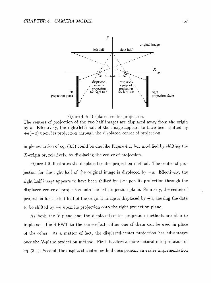
C H A P T E R 4. C A M E R A MODEL
original image
left half right half
Figure 4.9: Displaced-center projection. The centers of projection of the two half images are displaced away from the origin by a. Effectively, the right(1eft) half of the image appears to have been shifted by +a(-a) upon its projection through the displaced center of projection.
- / ./A.
d. - ..-Ye a . /
displaced ,/ center of
I projection ,' for right half
implementation of eq. (3.3) could be one like Figure 4.1, but modified by shifting the
- \ . X .
++ >
X-origin or, relatively, by displacing the center of projection.
Figure 4.9 illustrates the displaced-center projection met hod. The center of pro-
jection for the right half of the original image is displaced by -a. Effectively, the
right half image appears to have been shifted by +a upon its projection through the
displaced center of projection onto the left projection plane. Similarly, the center of
projection for the left half of the original image is displaced by +a, causing the data
to be shifted by -a upon its projection onto the right projection plane.
As both the V-plane and the displaced-center projection methods are able to
implement the S-RWT to the same effect, either one of them can be used in place
of the other. As a matter of fact, the displaced-center projection has advantages
over the V-plane projection method. First, it offers a more natural interpretation of
eq. (3.1). Second, the displaced-center method does present an easier implementation

CHAPTER 4. CAMERA MODEL 68
of the S-RWT. Consider that altering the parameter a in the S-RWT would change
the parameters r and 0 in the equations (4.12) and (4.15). This may involve adapting
the lens focusing in the V-plane projection (Figure 4.8).
In our design of the prototype RWT camera (Section 4.4.2), a combined use of the
patching and shifting methods is implemented to support the flexibility in dealing with
the singularity problem. The U-plane and the displaced-center projection techniques
are employed for the patching and shifting methods respectively.
4.4 A Prototype RWT Camera
The RWT is implemented as a lens projection between orthogonal planes under the
Sheimpflug condition [Bro65] discussed in Section 4.2.1. The lens focusing is modeled
with the first-order paraxial approximation. Practical considerations of various kinds
of lens aberrations become an issue when performing the actual design of the lens.
4.4.1 Periscopic lens design
As mentioned above, the first-order paraxial approximation is used to its advantage
for deriving the off-axis focusing. The lens aberrations thus encountered in off-axis
focusing are compensated with a careful lens design. In the RWT lens design, the pro-
jection between 90" planes imposes a stringent requirement on the lens performance.
Light rays reflected off the intermediate screen normally strike the RWT lens at a
wide-angled oblique incidence. Lens aberrations are adverse under such conditions.
As an initial attempt, we have chosen to use the periscopic lens as the candidate for
the RWT lens. The design data is generally available [Kin78]. The periscopic lens has
a symmetrical configuration of two meniscus-convex lens positioned on both sides of

CHAPTER 4. C A M E R A MODEL
a central stop (Figure 4.10).
The periscopic lens has the advantages that it has little distortion and lateral
color aberrations [Kin78]. Coma aberration can be ignored as it will be corrected
automatically by the symmetry of the lens configuration. Moreover, the field curvature
can be flattened by selecting the appropriate stop diameter. The periscopic lens is
shown to be necessary in our simulation tests. It will be shown later that when an
ordinary simple lens is used, the field curvature aberration causes poor focusing.
front-meniscus outer
inner
stop
rear-meniscus inner
outer
front-meniscus stop rear-meniscus
Curvature(cm-l) Separation(cm) Refractive Index
Figure 4.10: The periscopic lens and the lens design data. The effective focal length of the periscopic lens is 70 mm and the stop diameter is 8.87 mm.
4.4.2 Design of the RWT camera

CHAPTER 4. CAMERA MODEL
RWT lens
left intermediate
screen
. ,. .. .
right RWT left sensor /I! 1 \ RWT sensor
RWT *lens
6 T right intermediate screen
! mirror I ' P ' q
center-patch sensor
Figure 4.11: The RWT camera model The camera objective lens projects the image on the two intermediate screens on either side through the deflecting mirrors. The RWT lenses then focus the images from the screens onto the orthogonal RWT image planes. A center slot is opened between the deflecting mirrors enabling uniform-resolution projection onto the bottom wall. The full RWT image comprises segments from the RWT sensors on either side merged with the center patch from the bottom.

C H A P T E R 4. C A M E R A MODEL
The design of the camera is based on the model from the previous section. The light
rays are split into left and right halves by using the deflecting mirrors. A similar setup
of image splitting mirrors is also used in a stereo camera system by Teoh and Zhang
[TZ84], except that the deflecting mirrors used in our camera split the visual field in
the middle. The left field is projected onto the right screen and the right field to the
left screen. This facilitates the implementation of the two half planes in RWT to take
care of objects on each side of the visual field.
The two intermediate screens on either side of the camera play the role of the
object planes for the RWT lenses. Each RWT lens projects from the respective screen
onto an orthogonally located RWT image plane at the front wall of the camera. The
RWT transformation is realized by projection between these two orthogonal planes.
A practical consideration is how to take care of the singularity of the RWT at
x = 0. The patching and shifting techniques as discussed in Section 3.1.2 are employed
in this design. In Figure 4.11, a center slot is opened between the two deflecting
mirrors. Objects near to the optical axis (P3 and P4) are now projected to the center
of the bottom wall of the camera (pg and p4). As in the ordinary cameras, the image
at the center is a uniform-resolution projection.
To implement the shift parameter in eq. (3.3), a shift by a on the x-y images
from both intermediate screens needs to be performed. However, the shift can also
be realized by relative repositioning of the RWT lens. The lens is required to be
positioned at the X Y Z origin in Figure 4.5. Moving the lens and the projection
plane along the X axis in relation to the object plane effectively achieves the shifting
operation on the object's Xo coordinate. A shift by a on Xo thus causes eq. (4.8)
to realize the S-RWT which is defined in eq. (3.3). Practically, the RWT lens-sensor
units on either side of the camera in Figure 4.11 can be adjusted up and down in the

CHAPTER 4. CAA4ERA MODEL
diagram to implement the shift.
Now, three segments of the RWT image are formed at three locations. Merging
of the three pieces (left RWT, center patch, right RWT) will yield a connected image
like the bipolar RWT image shown in Figure 3.:3. Note that the sensors are delimited
in the way that the RWT image is continuous over the boundary between the left
and the center segments, and also between the center and the right segments. Proven
technologies from the 3-chip color cameras can be employed to deal with the problems
of synchronization and alignment among the three sensors.
Further design considerations for perfecting the camera design require deeper un-
derstanding of optical instruments. For example, a practical concern about the use
of the intermediate screens would be the weakness of the resulting irradiance a t the
RWT sensor planes after the diffuse reflection by the intermediate screens. The light
energy entering the camera through the field objective lens will get dispersed in all
directions due to the diffuse reflection by the screens. Consequently, only a small
portion of the energy will be collected by the RWT lenses and get projected onto
the sensor planes. Ultra-sensitive CCD sensors may be needed for recording the dim
image when it arrives at the end of the optical path.
Another concern is the diffraction effects caused by the center slot. When the slot
gets smaller, the diffraction effects become more eminent. Special measures may be
required to alleviate the diffraction or the foveal patch sensor should be mounted on
the side-wall alongside the screens to eliminate the need for the center slot altogether.
Despite all these detailed design considerations, the model depicted in Figure 4.11
is used to illustrate the basic principles of the optical construction which shows the
unique RWT projection and the implementation of the S-RWT and foveal patch. Any
practical design could be developed based on this basic model. In fact, camera design

C H A P T E R 4. C A M E R A MODEL 73
from this model would be appealing on three counts. First, the RWT obtains space-
variant resolution by using oblique projection between orthogonal planes. It does not
require sensing elements of variable sizes to achieve variable resolution. The main
advantage of using uniform sensors is thus realized. Second, the rectangular shape of
the sensors allows merging of the sensors to deliver a connected bipolar RWT image.
Third, the design accommodates a flexible implementation of both methods of S-RWT
and foveal patch. The foveal patch is adjustable by varying the aperture of the center
slot between the two deflecting mirrors. The shift parameter for the S-RWT can be
adjusted by shifting the RWT lens-sensor units.
Optical Simulations
Before a hardware prototype is built, the design for the RWT camera has been tested
using an optical ray tracing simulation software. The Beam Optical Ray Tracer2 is
used to provide a test environment in which the optics of lens refraction is simu-
lated. Since the optics of uniform-resolution projection for the center patch is well
proven in the conventional cameras, and since the optical path comprising the camera
objective through the intermediate screens is primarily adopted from the design of
ordinary stereo cameras, our tests are conducted mainly on the optics of the RWT
lens projection.
Our first experiment uses nine grid points placed on the object plane as shown
in Figure 4.12(a).~ Pencils of rays radiated from the points are propagated through
'Beam Optical Ray Tracer is the product of Stellar Software at Berkeley, CA, U.S.A., copyright 1990.
3Because it is easier to generate (or obtain) rectangular z-y images, they are used in this simula- tion. As a result, the generated RWT images are of the wedge shape. A real hardware RWT camera will have a rectangular sensor array and the corresponding view of the world will be of the wedge shape as pointed out in Section 3.1.3. Since T = T- l , the simulation result is equally valid.
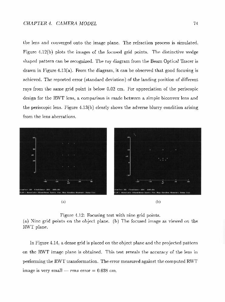
C H A P T E R 4. C A M E R A MODEL 74
the lens and converged onto the image plane. The refraction process is simulated.
Figure 4.12(b) plots the images of the focused grid points. The distinctive wedge
shaped pattern can be recognized. The ray diagram from the Beam Optical Tracer is
drawn in Figure 4.13(a). From the diagram, it can be observed that good focusing is
achieved. The reported error (standard deviation) of the landing position of different
rays from the same grid point is below 0.02 cm. For appreciation of the periscopic
design for the RWT lens, a comparison is made between a simple biconvex lens and
the periscopic lens. Figure 4.13(b) clearly shows the adverse blurry condition arising
from the lens aberrations.
Figure 4.12: Focusing test with nine grid points. (a) Nine grid points on the object plane. (b) The focused image as viewed on the RWT plane.
In Figure 4.14, a dense grid is placed on the object plane and the projected pat tern
on the RWT image plane is obtained. This test reveals the accuracy of the lens in
performing the RWT transformation. The error measured against the computed RWT
image is very small - rms error = 0.038 cm.

CHAPTER 4. CAMERA MODEL
Figure 4.13: Ray diagrams showing the lens focusing. (a) Good focusing is achieved with the use of periscopic design for the RWT lens. (b) Poor focusing arises from lens aberrations with the use of a simple biconvex lens. The ray diagram reveals the intolerable field curvature aberration.
Our experiment is concluded with a test on real image data. The assembly belt
image from the motion stereo experiments in [TL94] is used.4 Figure 4.15(a) is an
image of the assembly belt scene from the intermediate screen of the RWT camera
(it looks just like a normal uniform-resolution image), and Figure 4.15(b) is the RWT
image achieved through simulation on the RWT lens.
41n some applications, it is better to use only one half of the image where x > 0 (and hence u > 0). In this test case the origin is located at the middle of the left border in the original x-y assembly belt image. A small patch (6 = 15) at the left side of the x-y image is not transformed.

C H A P T E R 4. C A M E R A MODEL
Figure 4.14: Accuracy test on focusing using a dense grid. (a) A grid placed on the object plane. (b) The projected image as viewed on the RWT plane. The rms error measured against the computed RWT image is 0.038 cm.

CHAPTER 4. CAMERA MODEL
Figure 4.15: Focusing test using real data. (a) The belt image as view on the intermediate screen. (b) The image on the RWT plane.

Chapter 5
Applications of RWT Mapping
5.1 RWT Imaging in Road Navigation
In the problem of road following, an efficient search for road features can be effected
with the variable resolution offered by the RWT.
Different approaches have been devised for road detection in various experimental
autonomous land vehicles. An area-based voting scheme based on the Hough trans-
form is applied to compute the direction of the road in the CMU Navlab [THKS88].
In the VaMoRs project [DM92], visual features of the road edges are detected based
on the "Gestalt" hypothesis under adverse situations of shadows and absent lane-
markings.
Both methods search over the perspective images for road features. The drawback
is that the nearby section of the road gets overly attended whereas the far side toward
the horizon is disproportionately under-sampled. Arguably, this differential scale of
attention to detail is not suitable for driving on the road. One has to pay sufficient
attention to a reasonable distance to see the general direction of the road, while at
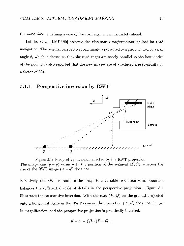
CHAPTER 5. APPLICATIONS OF RWT MAPPING
the same time remaining aware of the road segment immediately ahead.
Lotufo, et al. [LMD+SO] presents the plan-view transformation method for road
navigation. The original perspective road image is projected to a grid inclined by a pan
angle 6, which is chosen so that the road edges are nearly parallel to the boundaries
of the grid. It is also reported that the new images are of a reduced size (typically by
a factor of 32).
5.1.1 Perspective inversion by RWT
RWT plane
camera 0
0 . 0
0 . 0
0 , I
0 , 0 , I
0 /
I v ground . . . . . . . . . . . . . . . . . . . . . . . . . . . . . . . . . .
Figure 5.1: Perspective inversion effected by the RWT projection. The image size (p - q ) varies with the position of the segment (P, Q), whereas the size of the RWT image (p' - q') does not.
Effectively, the RWT re-samples the image to a variable resolution which counter-
balances the differential scale of details in the perspective projection. Figure 5.1
illustrates the perspective inversion. With the road (P, Q) on the ground projected
onto a horizontal plane in the RWT camera, the projection (p', q') does not change
in magnification, and the perspective projection is practically inverted.
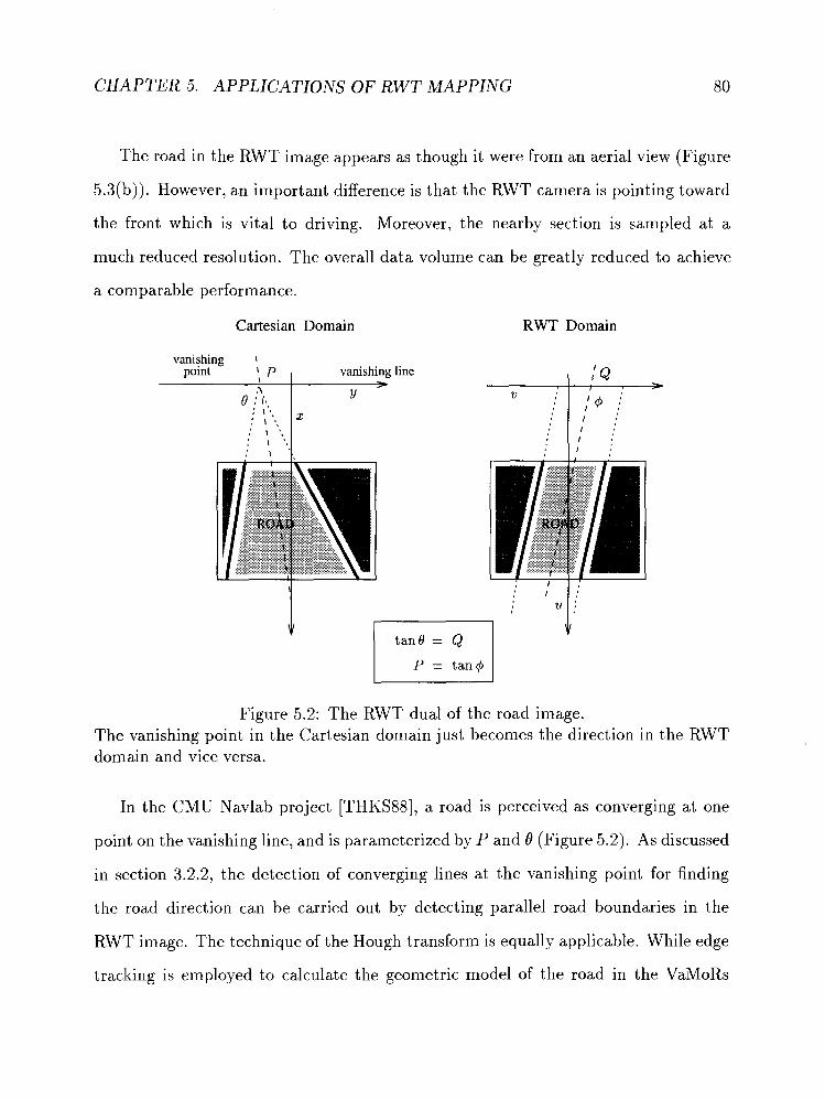
CHAPTER 5. APPLICATIONS OF RWT MAPPING 80
The road in the RWT image appears as though it were from an aerial view (Figure
5.3(b)). However, an important difference is that the RWT camera is pointing toward
the front which is vital to driving. Moreover, the nearby section is sampled at a
much reduced resolution. The overall data volume can be greatly reduced to achieve
a comparable performance.
Cartesian Domain RWT Domain
Figure 5.2: The RWT dual of the road image. The vanishing point in the Cartesian domain just becomes the direction in the RWT domain and vice versa.
In the CMU Navlab project [THKS88], a road is perceived as converging at one
point on the vanishing line, and is parameterized by P and 0 (Figure 5.2). As discussed
in section 3.2.2, the detection of converging lines at the vanishing point for finding
the road direction can be carried out by detecting parallel road boundaries in the
RWT image. The technique of the Hough transform is equally applicable. While edge
tracking is employed to calculate the geometric model of the road in the VaMoRs
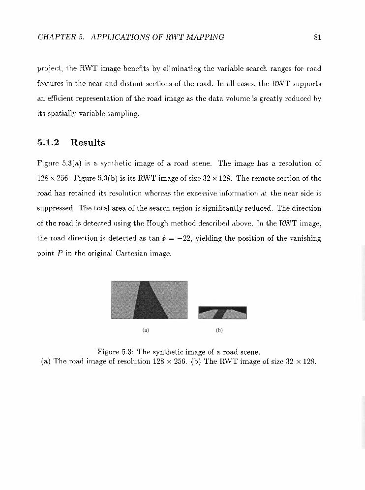
CHAPTER 5. APPLICATIONS OF R W T MAPPING 81
project, the RWT image benefits by eliminating the variable search ranges for roa,d
features in the near and distant sections of the road. In all cases, the RWT supports
an efficient representation of the road image as the data volume is greatly reduced by
its spatially variable sampling.
5.1.2 Results
Figure 5.3(a) is a synthetic image of a road scene. The image has a resolution of
128 x 256. Figure 5.3(b) is its RWT image of size 32 x 128. The remote section of the
road has retained its resolution whereas the excessive information at the near side is
suppressed. The total area of the search region is significantly reduced. The direction
of the road is detected using the Hough method described above. In the RWT image,
the road direction is detected as tan q5 = -22, yielding the position of the vanishing
point P in the original Cartesian image.
Figure 5.3: The synthetic image of a road scene. (a) The road image of resolution 128 x 256. (b) The RWT image of size 32 x 128.
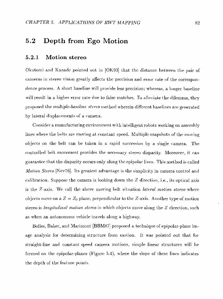
CHAPTER 5. APPLICATIONS OF R W T MAPPING
5.2 Depth from Ego Motion
5.2.1 Motionstereo
Okutomi and Kanade pointed out in [OK931 that the distance between the pair of
cameras in stereo vision greatly affects the precision and error rate of the correspon-
dence process. A short baseline will provide less precision; whereas, a longer baseline
will result in a higher error rate due to false matches. To alleviate the dilemma, they
proposed the multiple-baseline stereo method wherein different baselines are generated
by lateral displacements of a camera.
Consider a manufacturing environment with intelligent robots working on assembly
lines where the belts are moving at constant speed. Multiple snapshots of the moving
objects on the belt can be taken in a rapid succession by a single camera. The
controlled belt movement provides the necessary stereo disparity. Moreover, it can
guarantee that the disparity occurs only along the epipolar lines. This method is called
Motion Stereo [Nev76]. Its greatest advantage is the simplicity in camera control and
calibration. Suppose the camera is looking down the Z direction, i.e., its optical axis
is the Z-axis. We call the above moving belt situation lateral motion stereo where
objects move on a Z = Zo plane, perpendicular to the Z-axis. Another type of motion
stereo is longitudinal motion stereo in which objects move along the Z direction, such
as when an autonomous vehicle travels along a highway.
Bolles, Baker, and Marimont [BBM87] proposed a technique of epipolar-plane im-
age analysis for determining structure from motion. It was pointed out that for
straight-line and constant-speed camera motions, simple linear structures will be
formed on the epipolar-planes (Figure 5.4), where the slope of these lines indicates
the depth of the feature points.
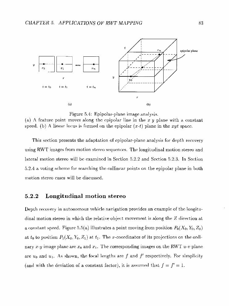
CHAPTER 5. APPLICATIONS OF RWT MAPPING
epipolar
/ plane
Figure 5.4: Epipolar-plane image analysis. (a) A feature point moves along the epipolar line in the x-y plane with a constant speed. (b) A linear locus is formed on the epipolar (x-t) plane in the xyt space.
This section presents the adaptation of epipolar-plane analysis for depth recovery
using RWT images from motion stereo sequences. The longitudinal motion stereo and
lateral motion stereo will be examined in Section 5.2.2 and Section 5.2.3. In Section
5.2.4 a voting scheme for searching the collinear points on the epipolar plane in both
motion stereo cases will be discussed.
5.2.2 Longitudinal motion stereo
Depth recovery in autonomous vehicle navigation provides an example of the longitu-
dinal motion stereo in which the relative object movement is along the Z direction at
a constant speed. Figure 5.5(a) illustrates a point moving from position Po(Xo, Yo, Zo)
at to to position Pl(Xo, Yo, Z1) at t l . The x-coordinates of its projections on the ordi-
nary x-y image plane are xo and xl. The corresponding images on the RWT u-v plane
are uo and ul. As shown, the focal lengths are f and f' respectively. For simplicity
(and with the deviation of a constant factor), it is assumed that f = f' = 1.
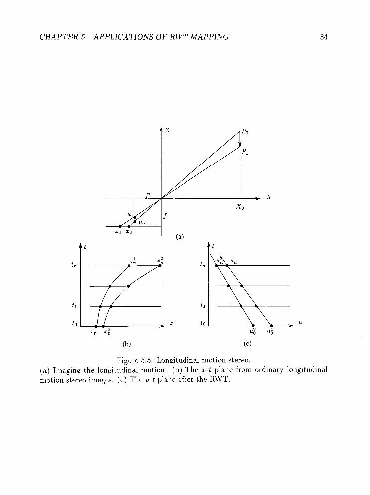
C H A P T E R 5 . APPLICATIONS OF R W T MAPPING
Figure 5.5: Longitudinal motion stereo. (a) Imaging the longitudinal motion. (b) The x-t plane from ordinary longitudinal motion stereo images. ( c ) The u-t plane after the RWT.
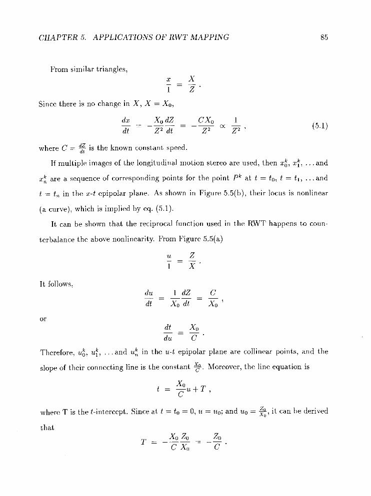
CHAPTER 5. APPLICATIONS OF R W T MAPPING
From similar triangles, x - - -
X -
1 Z
Since there is no change in X, X = Xo,
where C = 5 is the known constant speed.
If multiple images of the longitudinal motion stereo are used, then xk, x f , . . . and
2: are a sequence of corresponding points for the point Pk at t = to, t = t l , . . . and
t = t , in the x-t epipolar plane. As shown in Figure 5.5(b), their locus is nonlinear
(a curve), which is implied by eq. (5.1).
It can be shown that the reciprocal function used in the RWT happens to coun-
terbalance t he above nonlinearity. From Figure 5.5(a)
It follows,
Therefore, ut, u f , . . . and u t in the u-t epipolar plane are collinear points, and the
slope of their connecting line is the constant 5. Moreover, the line equation is
where T is the t-intercept. Since at t = to = 0, u = uo; and uo = a Xo ' it can be derived
that

CHAPTER 5. APPLICATIONS OF R W T MAPPING
This result immediately turns the problem of depth recovery in the longitudinal
motion stereo into a simpler problem of detecting lines in the u-t plane, where t-
intercepts are proportional to depth of the point Pk.
Extension to ego motion
In the following, the longitudinal stereo model is extended to a general case of ego
motion in which the vehicle is moving on the Y - Z plane with an axial velocity .i and
a rotational speed 8. Such a model typifies the road driving motion in which the
vehicle is curving along the road. Within a short time span, the vehicle motion can
be satisfactorily approximated with a circular course; that is, changes in both .i and
6 over the time span of investigation are assumed to be negligible.
R 1
I vehicle motion I
I
Figure 5.6: Motion of an object in relation to the vehicle. In the world coordinates, the vehicle is traveling at an axial velocity of .i and rotational speed of 6, describing a circular path of radius S/O. In the viewer-centered coordinates of the vehicle driver, the object is moving in the opposite direction with the same speed. It also appears to move on a circular trajectory at the same center.
Assuming the vehicle is moving in an otherwise static world, the apparent motion

CHAPTER 5. APPLICATIONS OF RWT MAPPING 87
of the world in the view of the vehicle driver is a composite motion of axial translation
-i and centric rotation -0. Take the vehicle driver as the center of reference and
align the Z axis with the direction of travel as depicted in Figure 5.6. At time t, the
position of the object is at (X, Y, 2 ) .
Solving the differential equations,
Y = R cos(do - 8t) - i / 0 ,
Z = Rsin(Oo - Ot) .
The form of the equations indicates a circular path for the object's apparent motion.
R is the radius of the circular path and the center is at Y = -.4/0, Z = 0. At
t = to = 0, the object is at the position (Yo, Zo), where Yo = R cos Oo - i / 0 and
Zo = R sin 00. Hence, Oo is the arc angle on the circular path at which the object is
initially located.
From Figure 5.5(a), the mapping from (Y, 2) to (u, v ) is
Apply the mapping on eq. (5.2-5.3). The image motion on the u-v plane now is
Let r = $ R and a = $8. The u-v motion equations can be rewritten as
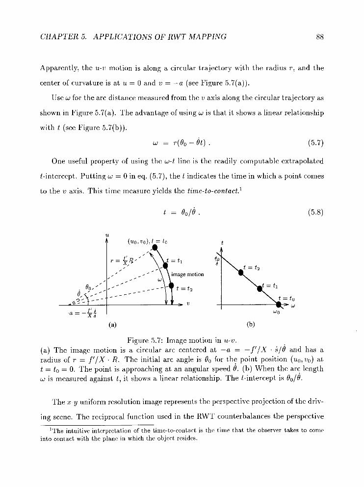
CHAPTER 5. APPLICATIONS OF RWT MAPPING 88
Apparently, the u-v motion is along a circular trajectory with the radius r , and the
center of curvature is at u = 0 and v = -a (see Figure 5.7(a)).
Use w for the arc distance measured from the v axis along the circular trajectory as
shown in Figure 5.7(a). The advantage of using w is that it shows a linear relationship
with t (see Figure 5.7(b)).
u = r(OO - Ot) . (5.7)
One useful property of using the w-t line is the readily computable extrapolated
t-intercept. Putting w = 0 in eq. (5.7), the t indicates the time in which a point comes
to the v axis. This time measure yields the time-to-contact.'
motion
t 2
v
Figure 5.7: Image motion in u-v. (a) The image motion is a circular arc centered at -a = - f ' / X i / B and has a radius of r = f ' / X - R. The initial arc angle is O0 for the point position (uo, vo) at t = to = 0. The point is approaching at an angular speed 6. (b) When the arc length w is measured against t , it shows a linear relationship. The t-intercept is Oo/6.
The x- y uniform resolution image represents the perspective projection of the driv-
ing scene. The reciprocal function used in the RWT counterbalances the perspective
'The intuitive interpretation of the time-to-contact is the time that the observer takes to come into contact with the plane in which the object resides.

CHAPTER 5. APPLICATIONS OF RWT MAPPING 89
nonlinearity and yields a linear mapping of the road surface (eq. (5.4)). The linear
mapping enables the preservation of the circular image motion as corresponding to
the original vehicle motion. Such is not the case in the x-y image because of the
perspective distortion
which results in a complicated movement on the x-y plane.
A search algorithm can be devised to find the circular trajectories on the u-v plane
as described in eqs. (5.5-5.6). When visualized in the 3-D uvt space, the circular
trajectory becomes a helical curve. The search is essentially a problem of fitting the
helical model to the uvt data. Nevertheless, the search space is much restricted by
exploiting the constraints due to the simple vehicle motion. The helical trajectory in
uvt has no more than two degrees of freedom even if none of the constants f', B, 0 are
known a priori. From eqs. (5.5-5.6), the center of the helix is on the v axis. Choose
a for the position of the center in eq. (5.6). The radius r and the arc length w for
each feature point (u, v , t ) from the RWT image sequence can be determined from
eqs. (5.5-5.7). The helical trajectory of the point (uo,vo) corresponds to a straight
line passing through wo in the w-t projection (Figure 5.7). Now, choose a value for the
line slope such that the line passing through wo would fit to the w-t projection of the
feature points. The best fitted line over different values of a yields the best solution
to the helical trajectory of (uo,vo). By eq. (5.8), the t-intercept of the w-t indicates
the time-to-contact.
The model of the longitudinal motion stereo for linear vehicle motion is a special
case of this general model for ego motion. When j -+ 0, 618 approaches m and so do
r and a in eq. (5.5-5.6). The circular trajectory therefore approaches a line along the
u direction, and the arc length w now directly corresponds to the u coordinate. In
C H A P T E R 5. APPLICATIONS OF R W T MAPPING 90
the general model, the t-intercept in w-t (eq. (5.8)) indicates the time-to-contact for
an object if the vehicle motion were to prevail. In the special case of linear vehicle
motion, the time-to-contact conveniently gives a direct measure of the depth of an
5.2.3 Lateral motion stereo
This section uses the example of the moving assembly line mentioned earlier. For
simplicity, we first assume that the belt moves in the X dimension in the 3-D space.
Its projected movement on the x-y plane is therefore along the x direction only. For
l k a point xk at y = y , x,, xf , . . .and xk is a sequence of corresponding points at
t = to, t = t l , . . .and t = t, in the x-t epipolar plane from the original (ordinary)
lateral motion stereo images, where the epipolar lines are horizontal (Figure 5.8(a)).
When the speed of the belt is constant and images are taken at equal intervals, xk,
xf , . . .and xk fall on a single line in the x-t plane, and % cx disparity d. Hence,
the correspondence problem in the lateral motion stereo is equivalent to a problem
of finding collinear points in the x-t epipolar plane. Since the disparity is inversely
proportional to the actual depth in the 3-D scene, it follows that cx depth of the
point xk.
After the RWT, the epipolar line corresponding to y = yhemains a line in the
u-v space, and v = ylu. The new epipolar line is generally at an angle with respect
to the u-axis passing through the origin. We denote the distance between the point
w(u , v) and the origin as w . For a point (x, y') on y = y',
The epipolar plane for the lateral motion stereo becomes the w-t plane as shown in

CHAPTER 5. APPLICATIONS OF RWT MAPPING
Figure 5.8: Epipolar planes in lateral motion stereo. - - -
(a) The x-t plane from ordinary lateral motion stereo images. (b) The w-t plane where
w = Jl+(y')Z/x. ( c ) The w-T plane where w = J m / x and r = t l x .

CHAPTER 5. APPLICATIONS OF RWT MAPPING 9 2
Figure 5.8(b). Note the new sequence of the corresponding points w,k, w,k, . . . and w,k
do not generally fall on a single line in the w-t plane.
Creation of a new w-T epipolar plane
To recover the linearity, an additional transformation
can be applied to the variable t which is similar to what is applied to y in the RWT.
The x-t epipolar plane from lateral motion stereo images is now converted into a new
W-T epipolar plane of the RWT images (Figure 5.8(c)). The horizontal epipolar lines
in the x-t plane become concurrent epipolar lines converging toward the origin in the
w-T plane. The lines that connect the corresponding points also remain linear.
Suppose LZt is a line in the x-t plane,
Its transformation dual (derivable from eqs. (5.9, 5.10)) in the w-T plane is L,,:
The slope m' of line Lxt becomes the T-intercept of L,, in the RWT motion st ere^.^
Instead of 2 m depth, it is now the case that the T-intercept of the line that connects
the corresponding points in the w-T plane is cx depth of the point wk.
Extension to any linear motion on Z = Zo plane
Although it was assumed above that the belt moves along the X dimension only, this
can be relaxed to any linear movement on a Z = Zo plane in the 3-D scene. The
?-This is similar to the transformation dual in eq. (3.4), except the slope of L,, is not c' because of the additional transformation on t (eq. (5.10)).

CHAPTER 5. APPLICATIONS OF RWT MAPPING 93
projected locus on the x-y plane is the epipolar line L,, of which the slope m and
y-intercept c are known parameters.
As shown by eq. (3.4), after the RWT the line L,, is transformed to the new line
L,, . Let ( be the length of the line segment L,, from the y-axis to (x, y ) ,
Apparently, ( and x have a linear relationship. A (-t epipolar plane (similar to the
x-t plane) can thus be constructed for the ordinary lateral motion stereo in which
corresponding points are collinear. Let the line that connects the collinear points in
the (-t plane be
L C t : t = m t - ( + c t . (5.12)
Now, let w be the length of the line segment L,, from the v-axis to (u, v),
Because u = l / x , use eq. (5.11),
If we introduce a new parameter T = t/(, then the line in the (-t plane (eq. (5.12))
will be converted into a line in the W-T plane,
In this way, the previous method for the lateral motion stereo can be extended to
handle known linear motions on any Z = Zo plane.
5.2.4 Search in the epipolar plane
As described above, the correspondence problem in both the longitudinal and lateral
motion stereo can be reduced to a problem of searching for collinear points in the

CHAPTER 5. APPLICATIONS OF RWT MAPPING 94
epipolar planes (u-t plane for the longitudinal, w-T for the lateral). Similar to the
procedures for the Hough transform [DH72], a voting algorithm for accumulating
multiple evidence can be developed. Without loss of generality, the search for linear
motion on the u-t plane in the longitudinal stereo will be used here to illustrate the
method. (The extension to circular ego motion requires a somewhat different search,
i.e., search for helical curves in the uvt space. By introducing w as the arc length, the
problem was shown in Section 5.2.2 to be equivalent to finding collinear points on the
w-t plane. For efficiency, a slightly different search algorithm was suggested earlier in
Section 5.2.2.)
In general, any point at t = ti can be paired with any point at t = t j ( j > i) to
form a hypothetical line segment. Its intercept on the t-axis suggests a possible depth
value which is inversely proportional to the disparity d. A 3-D uvd voting space is
created3 and each hypothetical line will cast a vote at the position (u, v, d) in the uvd
space. Since n + 1 collinear points can form 0 ( n 2 ) hypothetical lines and they will
vote to the same (u ,v , d), a peak will be formed in the uvd space which indicates
the consensus on the correct disparity value for the point (u, v). The line detection
problem can thus be solved by this voting procedure followed by a peak-detection
procedure.
On each u-t plane at t = ti there are ki edge points, i.e., u,l, ul, . . . and uft .
A complete pairing of two possible end points at ti and t j will produce numerous
hypothetical line segments and therefore clutter the uvd voting space. The following
heuristics are employed to improve the voting process:
Use relatively long hypothetical voting lines. Due to limitations of the
image resolution there is always some error in the u-v coordinates, especially at the
3Since the concerned depth in the scene can be very large whereas disparity d usually has a small range, it is preferable to use d for the voting space.

CHAPTER 5. APPLICATIONS OF RWT MAPPING 95
periphery of the RWT images. If the short hypothetical lines were to be used for
voting, a small amount of error in the u-v coordinates would result in relatively large
errors in the calculation of the slope and intercept, and consequently the disparity
values. A minimum length is therefore chosen to exclude the short voting lines.
Specify a reasonable range for depth. A range of concerned depth can be
represented as IT,;,, T,,,] to reduce the number of candidate pairs. The vertices T,;,
and T,,, on the t-axis and the lower end point ut form a triangle which defines the
search region for the possible pairing end point uj.
5.2.5 Experimental results
Longitudinal motion stereo
A vehicle navigation example is used to illustrate the longitudinal motion stereo.
Figure 5.9(a) shows a CMU image sequence of a road scene obtained from a driving
expedition. Four frames of the 8-snapshot sequence (each has a size of 512 x 512
pixels) are shown to visualize the forward motion from driving. The RWT images of
the motion sequence have been generated in software. The data reduction factor is
over 90%. Figure 5.9(b) shows the RWT edge images.
Some implementation details should be followed when generating the RWT images.
First, the X-axis in the world coordinate system is the vertical axis as indicated in
Figure 5.1. Accordingly, the x-axis in the x-y images and the u-axis in the RWT (u-v)
images are the vertical axes in these images. Second, the model of our longitudinal
stereo requires both the camera movement and its optical axis be along the Z-axis.
According to this simple model, the FOE (Focus of Expansion) is always at the
center of the x-y road images. When dealing with a FOE which is significantly off
center because of intentional pan/tilt on the camera orientation, the FOE must be

CHAPTER 5. APPLICATIONS OF R W T MAPPING
Figure 5.9: Depth computation using the RWT in linear motion.
(a) A sequence of a driving scene, only images 1, 3, 5 , and 8 are shown. (b) Edge images from the above RWT images. (c) Gray-level coded depth map computed from all eight images. (d) The depth map transformed back to the x-y space (uniform- resolution) for visual apprehension.

CHAPTER 5. APPLICATIONS OF RWT MAPPING
determined and used as the origin of the x-y space for the RWT transformation. This
is the situation in the CMU image sequence which apparently had the camera pointing
slightly toward the ground.
Even under the best effort to align the camera orientation with the vehicle move-
ment, the FOE could still be off center slightly. As a result, the epipolar line may not
align perfectly with the u-axis. To accommodate the resulting error, the search region
for collinear points used in the Hough method discussed in Section 5.2.4 has been re-
laxed accordingly. That is, instead of searching on an epipolar plane, a neighborhood
of the plane was employed as the search region.
In the images in Figure 5.9(b), some portions of the trees and buildings are not
shown, because they are either above the FOE or too close to the singularity (x = 0)
line to be included. The rest of the scene is very well captured in all the RWT images.
One can also observe the advantage of the variable-resolution imaging in this example
as the excessive details in the near side of the road, which are not as relevant to the
driving task, are averaged out in the coarse resolution periphery of the RWT images.
The algorithm described in Sections 5.2.2 and 5.2.4 has been implemented. The
correspondence ambiguities are resolved successfully and good depth recovery results
are obtained, Figure 5.9(c) shows the grey-level coded depth map. In Figure 5.9(d),
the RWT depth map is transformed back to the uniform-resolution x-y space so that
the relationship to the original road image can be better apprehended. Note that
the depth values of the traffic cones, the trash can and the tree trunks are correctly
resolved.

C H A P T E R 5. APPLICATIONS OF R W T MAPPING
Extension of longitudinal motion stereo to ego motion
A sequence of 20 motion images (400 x 494) of a table scene was taken in the lab
using the SFU hybrid pyramidal vision machine [LTR95]. Four of them are shown
in Fig. 5.10(a). The camera was mounted on the NOMAD 200 mobile robot. The
NOMAD was moving forward while turning left.
As before, the X-axis in the world coordinate system, the x-axis in the x-y images
and the u-axis in the RWT (u-v) images are the vertical axes.
By calibrating the camera it is determined that the Y - Z plane on which the camera
makes the circular movement is slightly below the whiteboard. In this way, the y-axis
(where x = 0) on the x-y image is determined. The center of the axis is taken as
the origin for the RWT. The whiteboard in the scene is above the origin which is
not in the lower half of the x-y image in consideration here. Fig. 5.10(b) shows the
edge maps for the RWT images for the lower half of the table scene. As before, the
top portion of the tape boxes and cup are excluded because they are too close to the
origin. The effect of spatially variable-resolution sensing is apparent. In this case, the
front edges of the table are in the periphery and compressed in the RWT images.
Since the projections of the movement in the uvt space follow a helical curve,
search is conducted along such possible curves in the 3-D uvt space, which reduces the
complexity of matching significantly. For a given a and (uo, vo), the helical trajectory
is well-defined and incurs little ambiguity in possible matching candidates on the
locus. After gathering the matching points, their arc length w is calculated and used
to derive the "time-to-contact". Fig. 5.10(c) is the grey-level coded map of time-to-
contact in the RWT domain and Fig. 5.10(d) is the map in the original x-y domain
generated by an inverse RWT.

CHAPTER 5. APPLICATIONS OF R W T MAPPING
Figure 5.10: Analysis of ego motion. (a) A dynamic sequence of an office scene, only images 1, 7, 13, and 19 are shown. (b) Edge images from the above R,WT images. ( c ) Map of time-to-contact computed from all twenty images. (d) Map of time-to-contact transformed back to the x-y space.

C H A P T E R 5. APPLICATIONS OF RWT MAPPING
Lateral motion stereo
For obtaining lateral motion stereo images in our lab, a pyramidal wooden block is
placed on a conveyor belt that moves from left to right. A sequence of eight snapshots
(each has a size of 512 x 512 pixels) from a conventional CCD camera is used in the
experiment (Figure 5.11(a)) since the RWT camera is not available yet. As before,
the RWT images (Figure 5.11(b)) are generated in software by mapping the original
images from x-y to u-v. The middle point of the left boundary of the x-y image plane
is used as the origin for this mapping. In our experiment, the area of the resulted
RWT images is chosen at approximately 1/10 of the original images.
Gradient-based edge detection is first performed on the RWT images. Figure
5.11(c) shows the edge map from the first RWT image. Collinear points in the w-r
plane are detected and their T-intercept yields the depth and, indirectly, the dispar-
ity. The voting in the uvd accumulator space results in clusters yielding the correct
disparity. Figure 5.11(d) displays the depth map. The result shows that most of the
disparity changes along the edges of the pyramid are computed successfully.
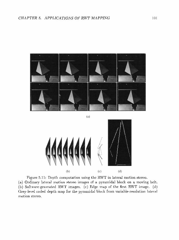
CHAPTER 5. APPLICATIONS OF RWT MAPPING
Figure 5.11: Depth computation using the RWT in lateral motion stereo. (a) Ordinary lateral motion stereo images of a pyramidal block on a moving belt. (b) Software-generated RWT images. (c) Edge map of the first RWT image. (d) Grey-level coded depth map for the pyramidal block from variable-resolution lateral motion stereo.

Chapter 6
Active Stereo
Binocular Vision in Space-variant Sensing
Experiments have shown that the human stereopsis accepts only a very limited range
of disparities. The Panum's area forms a limited zone about the fixation point. Be-
yond the Panum's area, we can no longer fuse the stereo images. In computer vision,
stereo correspondence is linked to the fusion of two disparate retinal images. The
problem is formulated as computing the image disparity within an operating range.
Correspondence algorithms are normally incorporated with the various matching
constraints to render the problem solvable. Uniqueness, continuity [MP76], and the
figural continuity [MF81] are the commonly used ones. Burt and Julesz [BJ80b] con-
ducted some experiments on fusion in the context of disparity gradient. An amend-
ment to the previous understanding of Panum's fusional area was made. Binocular
fusion occurs only when the disparity gradient does not exceed a critical value of - 1.
Li [Li94a] generalized the notion of disparity gradient to subsume various constraints
for stereo matching.
CHAPTER 6. ACTIVE STEREO
After more than three decades of intensive research in stereo vision, the compu-
tational framework for stereopsis from uniform resolution images has been relatively
well-established. The link to psychological vision is that correspondence is computed
as the fusional result, and the disparity yields the 3-D percept. As the methods
devised are mostly for accurate recovery of the image disparity, the process can be
considered as computing the foveal fusion in the domain of space-variant sensing.
However, the structure and functional objective of the peripheral vision are distin-
guished from those of the foveal processing. The issues of peripheral fusion have not
received much attention. This may be in part due to the lack of research in anthro-
pomorphic sensors. With the invention of the space-variant sensor [VdSKCS89], the
issues related to active stereo has received attention in recent years.
In this chapter, we shall investigate the Panum's fusion in the context of space-
variant binocular sensing. Specifically, the computational view of the Panum's fusional
area in the space-variant RWT sensing space will be studied, and a model of the
fixation mechanism in an RWT binocular system will be presented.
6.1.1 Panum's fusional area
Objects on the horopter form stereo images on the corresponding retinal elements
in the two eyes. Images of zero disparity as such are perfectly fusible, and are seen
single. Panum (1861) showed that zero disparity is not the necessary condition for
singleness [Og164]. An image on one eye would fuse with a similar image on the retina
of the other eye within a small area about the corresponding point.
Consider the zero disparity case. Suppose the eyes are fixating an object PHoTopter
(Figure 6.1). PHoTopteT is on the horopter. The object forms zero disparity images in
the two eyes, and thus is seen single. Another object PI,,,, is located to the inner

CHAPTER 6. ACTIVE STEREO 104
side of PHoTopteT. As PI,,,, is moved towards the viewer, at a certain point, one will
no longer be able to fuse the images and start to see double. Similarly, the object
Pouter to the outer side of PHoTopteT is seen double when it is sufficiently away from
the horopter. This type of doubling is known as physiologic diplopia. The images
produced are said to be crossed disparate, and uncrossed disparate, respectively. The
interval between PI,,,, and Pout,,, where no doubling is seen, defines the limits of
the Panum's fusional area.
Panum's area Outer limit I \
a I \
Uncrossed disparate
00 L R
Horopter .
Inner limit
Left eye Right eye
Figure 6.1 : Panum's fusional area.
Zero disparity
0
Crossed disparate
00 R L
-
Within a region about the horopter, disparate images are fused despite their images not falling on the corresponding retinal elements. To the outer side of the Panum's area, uncrossed disparate images are seen. Objects to the inner side yield crossed disparate images.

CHAPTER 6. ACTIVE STEREO
In human vision, it is functional to address only a small range of disparities near
the fovea because thereby one can filter out the irrelevant visual information and
concentrate on the object of interest about the fixation point. One wants to keep
a visual account, albeit coarse, of the environment in the visual periphery, because
monitoring of the general environment is crucial for smooth ego motion and fast
response to impending activities. Quantitative studies by Fischer (1924) and Ames
(1932) yield data that plot out the size of the Panum's area at different visual angles
[Og164]. Fender and Julesz [FJ67] reported that binocular fusion occurs in regions
vary from 6 min. of arc at the center of the visual field to 20 min. of arc at the
peripheral angle of 6".
An extended Panum's fusional area is perhaps ideal for accurate spatial perception
of the scene. However, it is unrealistic because it represents too great a demand on the
fusion process, as fusion would be expected to be performed over an excessive range of
disparity. Olson [Ols93] believed that stereopsis plays an ecological role of privileged
computational resource, like the fovea that provides information about fixated targets
only. The severe limitation of the size of the Panum's area is seen as beneficial, since
binocular single vision is focused on the fixated target while stimuli from the rest of
the scene are largely filtered out as irrelevant.
While Olson compares the role of Panum's area to the functional value of the
retinal fovea, we relate the rapid dilation of the Panum's area at the peripheral visual
angles to the coarse sensor resolution at the retinal periphery. When one interacts
with the environment, accurate foveal processing serves well for attentive inspection
of the fixated target. However, general monitoring of the wide visual field is obviously
important for detection of activities, smooth maneuvering and the spatial percept of
the external environment.
CHAPTER 6. ACTIVE STEREO 106
In this thesis, a functional perspective that relates the spatial extent of the Panum's
area to space-variant sensing resolution is adopted. A uniform resolution image does
not meet the requirements of this fovea-periphery structure for visual processing. It
has neither the sufficient resolution for foveal vision, nor the coarse resolution for
peripheral processing. In particular, to achieve a deep sensing range at large eccen-
tricity, the disparity calculation has to be carried out over an excessively wide range.
This is because the uniform resolution image data contain information far too detailed
for peripheral vision purposes. In this respect, the space-variant resolution is highly
desirable. The RWT image is suitable for space-variant processing as it can support a
good foveal resolution and, at the same time, a desired level of coarse resolution in the
periphery. Furthermore, the RWT simplifies the disparity computation because its
variable resolution is affected primarily in the horizontal dimension. The horizontal
displacement inflicted in stereo images due to the binocular disparity is well captured
in the RWT representation.
6.2 Computational Model for Binocular Fixation
6.2.1 Fusional range in RWT
In computer vision, the fusional range is computationally modeled by disparity limits.
Olson and Coombs [OC91, CB921 perform real-time pursuit on a fixated object by
running a near-zero-disparity filter on the stereo images. The verging system of Olson
[Ols93] operates in a limited range of disparities (-3 to 3). Based on the studies of
anomalous stereopsis [Ric71], Barnard [BF90, Bar901 computes image disparities at
3 values only, namely 1 for crossed disparate, 0 for near-zero disparity and -1 for
uncrossed disparate images.
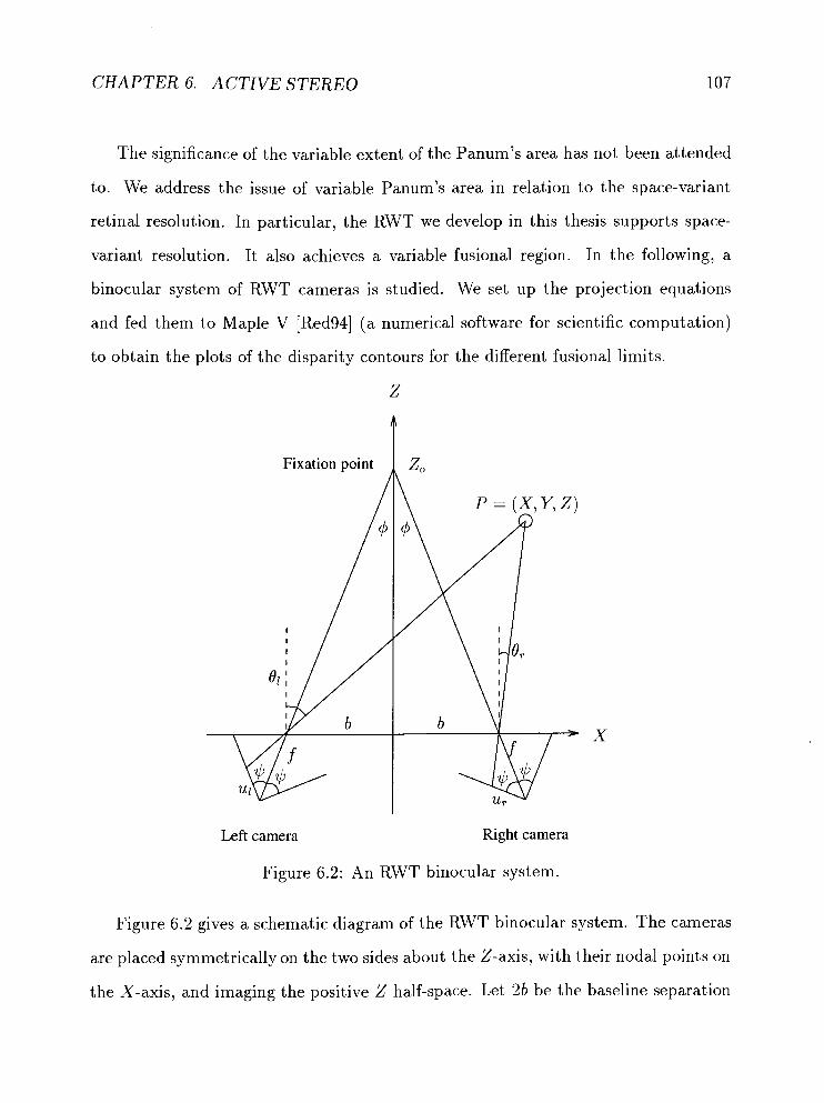
CHAPTER 6. ACTIVE STEREO 107
The significance of the variable extent of the Panum's area has not been attended
to. We address the issue of variable Panum's area in relation to the space-variant
retinal resolution. In particular, the RWT we develop in this thesis supports space-
variant resolution. It also achieves a variable fusional region. In the following, a
binocular system of RWT cameras is studied. We set up the projection equations
and fed them to Maple V [Red941 (a numerical software for scientific computation)
to obtain the plots of the disparity contours for the different fusional limits.
z
Fixation point
Left camera Right camera
Figure 6.2: An RWT binocular system.
Figure 6.2 gives a schematic diagram of the RWT binocular system. The cameras
are placed symmetrically on the two sides about the Z-axis, with their nodal points on
the X-axis, and imaging the positive Z half-space. Let 2b be the baseline separation

CHAPTER 6. ACTIVE STEREO 108
of the cameras. The focal length of the cameras is denoted by f , and the inter-
projection-plane angle is 24. The cameras are fixating the point Zo on the Z-axis.
Let P be a point located at (X, Y, 2); ul and u, are the RWT coordinates of the
left and right images of P respectively. Let the disparity be denoted by d. The
triangulation geometry in Figure 6.2 yields the following equations:
The system of equations are solved for X and Z at different disparity values, d.
Without loss of generality, set b = 200, f = 200, 4 = 45O, and Zo = 6000 (in 1/100
inch unit). The numerical values of X and Z are calculated for d ranging from -4
to $4. Figure 6.3 plots the (X, Z ) coordinates for d = 0, f 2, f 4. Each of the curves
represents a disparity contour of a particular d. All points on the same contour
will form disparate images in the two RWT cameras with the disparity d. These
contour are due to the specific imaging configuration of the RWT binocular system.
However, the corresponding fusional region indeed exhibits the desired property of
fovea-periphery variable extent. In this example, the fusional region at the peripheral
angle of 36" is twice as deep as that at the central position.
Comparison of the RWT binocular system are drawn with the conventional uniform-
resolution cameras. The model of a verging system of uniform-resolution cameras is

CHAPTER 6. ACTIVE STEREO
Figure 6.3: Disparity contours for the RWT binocular projection. The plot is obtained by setting the baseline separation 2b = 400, the focal length f = 200, and the inter-plane angle q5 = 45'. The cameras are converged at the fixation point of 6000 on the cyclopean axis. From the outermost contour to the innermost one, the disparity contours are plotted in the order of d = $4, +2,0, -2, -4.
given in Figure 6.4. This time, the set of equations yielded read as follows:
Again, the system of equations are solved in Maple V for X and 2. Similarly, a plot
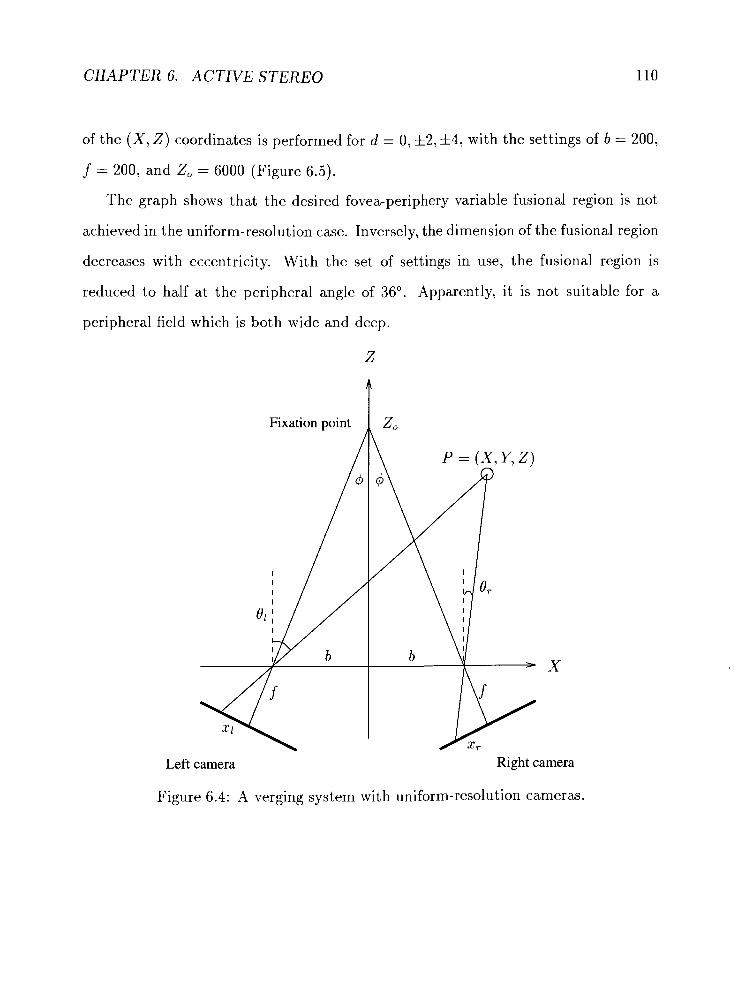
CHAPTER 6. ACTIVE STEREO 110
of the (X, 2) coordinates is performed for d = 0, f 2, f 4, with the settings of b = 200,
f = 200, and 2, = 6000 (Figure 6.5).
The graph shows that the desired fovea-periphery variable fusional region is not
achieved in the uniform-resolution case. Inversely, the dimension of the fusional region
decreases with eccentricity. With the set of settings in use, the fusional region is
reduced to half at the peripheral angle of 36'. Apparently, it is not suitable for a
peripheral field which is both wide and deep.
z
Fixation point
1 / Left camera Right camera
Figure 6.4: A verging system with uniform-resolution cameras.
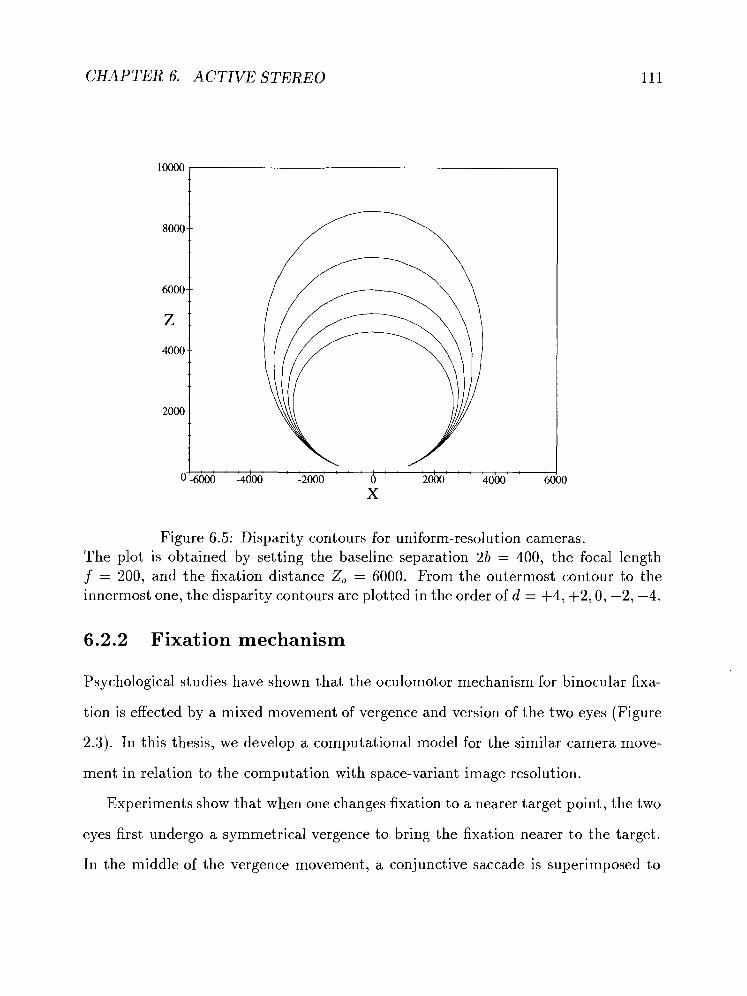
CHAPTER 6. ACTIVE STEREO
Figure 6.5: Disparity contours for uniform-resolution cameras. The plot is obtained by setting the baseline separation 2b = 400, the focal length f = 200, and the fixation distance Z,, = 6000. From the outermost contour to the innermost one, the disparity contours are plotted in the order of d = +4, +2,0, -2, -4.
6.2.2 Fixat ion mechanism
Psychological studies have shown that the oculomotor mechanism for binocular fixa-
tion is effected by a mixed movement of vergence and version of the two eyes (Figure
2.3). In this thesis, we develop a computational model for the similar camera move-
ment in relation to the computation with space-variant image resolution.
Experiments show that when one changes fixation to a nearer target point, the two
eyes first undergo a symmetrical vergence to bring the fixation nearer to the target.
In the middle of the vergence movement, a conjunctive saccade is superimposed to
CHAPTER 6. ACTIVE STEREO
swing the gaze in line with the target. The vergence then proceeds to completion in
the final stage to bring the fixation accurately to the target.
If cameras of uniform sensing resolution were used, the binocular fixation process
would be much simplified. Shifting from one fixation to another would involve calcu-
lating the exact image disparity and angular position of the target. The process could
then be accomplished by generating independent pan-tilt movement to each camera,
since it is possible to complete exact calculation for the target at the previous fixation.
To assume such a retina, ignores all the problems ranging from hardware requirements
to processing complexity. After all, to make such an assumption would beg the ques-
tion of whether the fixation process was genuinely necessary to perception, since the
high resolution sensory data of the scene is already available without the need for
specific gaze control.
There is no doubt that uniform resolution cameras could hardly be supported. In
fact, it is apparent that there is a strong relevance of space-variant sensor resolution
to the unique camera movement for binocular fixation.
From the computational point of view, space-variant sensor resolution supports
fusional area of variable size. This is because a disparity near the point of fixation
yields refined and narrow depth range; whereas, the same disparity at the periphery
corresponds to an coarse but deep depth range. Thus, the variable fusional area is
not only functional, it also represents a logical structure in space-variant sensing.
The unique camera movement now becomes natural in a binocular system with
space-variant sensors. Consider the case when the cameras are fixating an object A
in the scene, and is about to change gaze to a nearer one B at periphery. A is fixated
in the fusional region at the fovea. B, although located in the periphery, is covered
in a deeper fusional area. Computationally, the fusional area's limit is used to the

CHAPTER 6. ACTIVE STEREO 113
advantage for restricting the disparity range. Under the limited operating range for
disparity, B's disparity is readily resolvable even though its depth differs very much
from that of the fixation. If the cameras were straightforwardly gazed at B at this
time, B might become out of the fusional limit when it is brought into the foveal
direction. The depth of B would be difficult to calculate and the fixation would fail.
A more effective mechanism is to have a first vergence to change the fixation distance
so that B is lying close to the horopter after the vergence. This also prepares for the
versional movement so that when B is brought to the foveal direction, it will still be
imaged within the fusional limit. Next, based on the rough estimate of B's visual
angle, a pan movement is launched to direct both cameras to the direction near B.
Now, B is in a near-foveal direction, and located wit,hin the fusional limit. This is
true owing to the first vergence. Finally, a second vergence can be executed to bring
B accurately into fixation.
Figure 6.6 summarizes the camera movement of a space-variant binocular sensor.
As a matter of fact, it resembles the eye movements observed in the human visual
system [Yar57] (Figure 2.3).
6.3 Binocular Fixation using RWT Images
RWT fits in the model described above. The RWT supports a space-variant sensing
resolution. As we have discussed, the unique camera movement of binocular fixation
is closely related to space-variant sensor resolution.
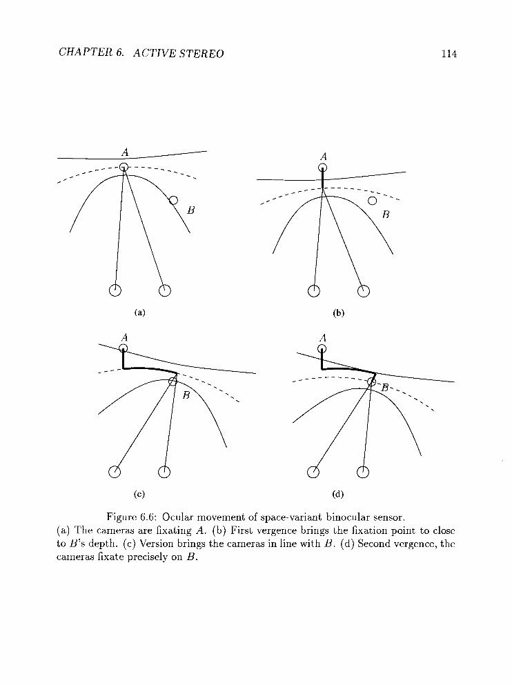
CHAPTER 6. ACTIVE STEREO
Figure 6.6: Ocular movement of space-variant binocular sensor. (a) The cameras are fixating A. (b) First vergence brings the fixation point to close to B's depth. (c) Version brings the cameras in line with B. (d) Second vergence, the cameras fixate precisely on B.

CHAPTER 6. ACTIVE STEREO
6.3.1 Disparity cornputat ion
Another property that renders RWT suitable for stereo vision is the anisotropy of
its space-variant resolution. In stereo vision, the disparate images formed in the
binocular cameras differ from each other by a horizontal displacement. It is this
disparity that indicates the depth of the imaged object. In the conventional images,
disparity is computed by correlation along the horizontal dimension. A rectangular
pattern in the Cartesian image appears as shifted along the horizontal streamlines
(Figure 6.7(a)). Recall from Section 3.2.1, the horizontal streamlines are mapped to
radials in the RWT domain. Figure 6.7(c) shows the bipolar RWT image. The radial
streamlines converge at the two antipodes on the u-axis. In the RWT image, the
rectangular pattern is transformed into a wedged rectangle displaced along the radial
streamlines.
Disparity computation may become very complicated in other schemes of image
representation. In the log-polar model, horizontal streamlines are mapped to com-
plicated log-sine curves (Figure 6.7(b)). The difficulty is at least two-fold. First of
all, disparate images are not related in a linear structure any more. Search for stereo
correspondence has to be conducted along these log-sine curves which are expensive
to compute. In addition, the image pattern gets rotated and scaled while being trans-
lated along the log-sine curve. A complicated procedure is required to calculate the
image motion in order to make it possible for a correlation operator to be used for
the disparity computation [GLW92].
The anisotropic property of the RWT space-variant resolution effects the mapping
primarily along the x dimension only. The y dimension is largely unaffected except by
being scaled according to l /x . The verticals in the x-y grids are invariantly mapped
to verticals. The horizontals are mapped into radial lines. In spite of that the image
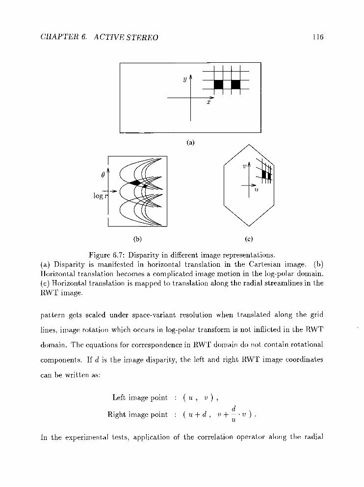
CHAPTER 6. ACTIVE STEREO
Figure 6.7: Disparity in different image representations. (a) Disparity is manifested in horizontal translation in the Cartesian image. (b) Horizontal translation becomes a complicated image motion in the log-polar domain. (c) Horizontal translation is mapped to translation along the radial streamlines in the RWT image.
pattern gets scaled under space-variant resolution when translated along the grid
lines, image rotation which occurs in log-polar transform is not inflicted in the RWT
domain. The equations for correspondence in RWT domain do not contain rotational
components. If d is the image disparity, the left and right RWT image coordinates
can be written as:
Left image point : ( u , v ) , d
Right image point : ( u + d , v + - v ) . U
In the experimental tests, application of the correlation operator along the radial

CHAPTER 6. ACTIVE STEREO
streamlines yields good estimates of the RWT image disparities.
6.3.2 Fixation transfer
For simplicity, the correlation method is used as an operator for disparity computation.
A windowed correlation is performed on the RWT stereo images within a limited
operating range of disparity that corresponds to the space-variant fusional area.
In an RWT binocular system, when changing from the current fixation to another
target at the visual periphery, the model for camera movement described in Section
6.2.2 is followed. A variable fusional area results from the space-variant pixel reso-
lution. Upon changing gaze from the current fixation point to the next target, the
target may be located well within the fusional limit at the periphery. A rough es-
timate for the target's peripheral disparity is calculated. The two cameras are then
converged/diverged to reduce this disparity. This corresponds to the first vergence
movement. Next, the cameras are panned to the viewing angle of the target to bring
the target to the fovea of the RWT cameras for higher resolution imaging. This opera-
tion corresponds to the versional movement. The target now in the foveal direction of
the cameras is likely imaged with a residual foveal disparity. Correlation is performed
in the fovea. Based on the resulting disparity the cameras are convergedldiverged to
zero in on the target precisely. This movement corresponds to the second vergence.
Figure 6.8(a-d) shows a test on a computer simulation of the fixation process in
an RWT binocular system. An office scene is originally imaged with a camera at two
viewing positions. In the simulation, pan-tilt movements of the camera are simulated
by centering the image at the appropriate pixel. Figure 6.8(a) shows the images
corresponding to a fixation on the computer keyboard in the office scene. It shows
the RWT images of the scene and the disparity map. These RWT images are the data

CHAPTER 6. ACTIVE STEREO
used in the actual computation. The Cartesian edge map is also shown here for the
reader's apprehension of the disparate scene images and the camera orientations.
As the chair is located at a closer range to the cameras in relation to the keyboard
(the current fixation point), it exhibits a non-zero disparity. The disparity value,
however, is small as it is located in the periphery. The image disparities in this
example are well within the fusional limit. The disparities are computed by applying
a 3 x 3 windowed correlation over a range of [-5,5]. The disparity results reveal
different disparities for objects at different depth from the keyboard. The chair has a
large crossed disparity whereas the magazine organizer on the desk shows a non-zero
uncrossed disparity.
The fixation exercise in this test is to change the gaze from the computer keyboard
to the chair. Three intermediate steps are involved. Initially, the cameras are fixated
at the keyboard. A disparity of -4 is detected with the chair at a peripheral angle
corresponding to u = -72 pixels. By the RWT inverse transformation, a -4 disparity
at u = -72 is translated back to the Cartesian domain to a disparity of -10 pixels at
x = -101. Should there be a real hardware camera control to the binocular system,
a mapping function is required to map the -10 disparity to the disjunctive vergence
angle that converge the cameras so that the peripheral disparity of the chair image
becomes zero. In this exercise, the vergence is simulated by re-centering the left
Cartesian scene image by 5 pixels to the right and the right scene image by 5 pixels
to the left. The RWT images are then obtained from the Cartesian scene images for
the new camera orientations as though they are from the real RWT cameras. Figure
6.8(b) now shows the result of the first vergence. The chair images at u = -70 are
now well aligned as seen in the edge map in (b), and the disparities shown in the
disparity map demonstrate that zero disparity is achieved with the chair images.

CHAPTER 6. ACTIVE STEREO
Next, the cameras are panned to the left for an angle corresponding to 72 pixels in
the RWT domain. Again, this is accomplished by re-centering both Cartesian images
by 101 pixels to the left. Figure 6.8(c) shows the result of this conjunctive versional
movement. The chair images now come to the foveal region of the cameras. It is
observable that the estimate for the peripheral disparity during the first vergence is
not accurate enough for high resolution processing inside the fovea. The disparity
map in (c) shows that the residual disparity in the chair images becomes apparent
once they are shifted to the fovea. This foveal disparity, however, has a value well
within the operating range of the fusional limit since the first vergence has already
achieved a good approximation.
Figure 6.8(d) now takes the vergence to completion. The foveal disparity of the
chair is computed. It is a small residual disparity of 1 pixel. The cameras are then
diverged by an angle corresponding to 1 pixel in the RWT images. Carried out in
simulation, the right Cartesian scene image is re-centered by 1 pixel to the right. The
RWT is applied to obtain the new images as the result of the second vergence. The
disparity map in (d) shows that the cameras are precisely fixating the chair in the
fovea.
The RWT supports the fixation mechanism in an effective way. If fixation were
performed on the conventional uniform-resolution image data, large disparities would
have to be calculated. Eminent problems associated with large disparity, such as
multiple ambiguous matches and slow computation have to be resolved.
6.3.3 A system view
This thesis reports on the design and simulation of a system for the interactive fixa-
tion process described above. Figure 6.9 shows the system. It comprises the vergence

CHAPTER 6. ACTIVE STEREO 120
edge map
left RWT right RWT
disparity
Figure 6.8: (a) Fixation sequence. Initially, fixation is on the computer keyboard.
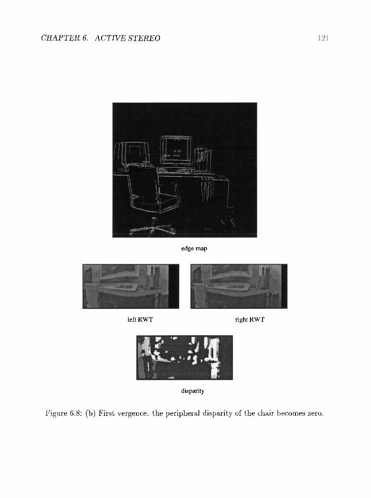
CHAPTER 6. ACTNE STEREO
edge map
left RWT right RWT
disparity
Figure 6.8: (b) First vergence. the peripheral disparity of the chair becomes zero.

CHAPTER 6. ACTIVE STEREO
edge map
left RWT right RWT
disparity
Figure 6.8: (c) Version. The chair is brought to the fovea.
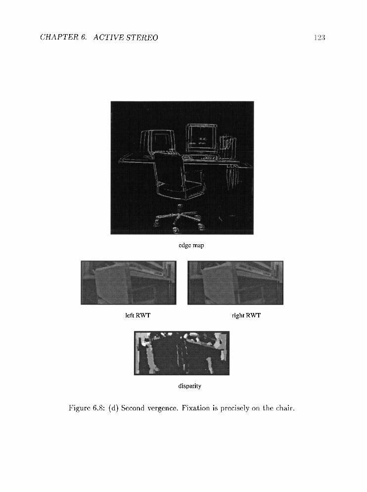
CHAPTER 6. ACTIVE STEREO
edge map
left RWT right RWT
disparity
Figure 6.8: (d) Second vergence. Fixation is precisely on the chair.

CHAPTER 6. ACTIVE STEREO
and version components interfacing with the controller of the camera pan-tilt plat-
form. The next fixation which initiates vergence and version oculomotor sequence is
computed by the "where-next" component. Vergence is a slow and visually guided
process. It is adjusted according to the disparity, thus completing the feedback loop.
The camera platform houses two cameras each of which has the two degrees of
freedom for pan and tilt respectively. Examples of pan-tilt platforms can be found
in the previous research [CB92, Kro89, AA93, PUE931 and the reports collected in
[CBB93]. In our system, the cameras are RWT cameras which output RWT images of
the scene directly. If ordinary cameras were used, the RWT images could be generated
from the uniform-resolution images with a Reciprocal-Wedge transformation routine.
The gaze angles for vergence and version are mapped to the mechanical movements
of pan and tilt for individual camera. The version angle drives identical movements
of pan and tilt for both cameras, whereas the vergence is split evenly into disjunctive
convergence or divergence between the two cameras.
The component "where-next" represents the high-level intelligent process for se-
lecting the next fixation point in the scene. The left and right RWT images are
combined to yield a cyclopean image of the scene (for convenience the left image is
used in our simulation). The "where-next" component searches in this cyclopean im-
age for features of interest. In fact, the next-fixation computation is a highly involved
process [Yar67]. Although this high-level intelligent process for computing the next
fixation is an interesting topic for research, it is beyond the scope of this thesis. In
the fixation exercise which involved shifting attention from the computer keyboard
to the office chair, the next fixation (the chair) is actually typed in by hand. In the
following demonstration of an active fixation system, simplistic heuristic criteria are
used to show the usual scanpath behavior in binocular visual exploration.

CHAPTER 6. ACTIVE STEREO
Once the next fixation has been decided, vergence and version are initiated. Dif-
ferent strategies are employed when computing disparities in the foveal and peripheral
regions. Area-based techniques are used in the peripheral regions and feature-based
techniques are used in the foveal region. As image data are imprecise under the coarse
resolution and reduced size in the peripheral regions, accurate localization of fine fea-
tures is not expected. Area-based windowed correlation techniques matching image
areas are more appropriate at the periphery. Inside the fovea, acute sensitivity is facil-
itated. More sophisticated feature-based techniques can be employed. Edge features
are detected and matched with attributes such as edge orientation and gradient.
In Figure 6.9, two disparity modules are simulated, namely the peripheral dis-
parity and foveal disparity described above. The former is used in the first vergence
to eliminate the peripheral disparity. The latter is used in the second vergence to
converge precisely on the target inside the fovea.
The position of next fixation is used to drive the versional movement. Synchronous
panning motion is produced to swing the cameras in line with the target. Due to
the coarse resolution in the periphery, the initial estimate for the magnitude of the
panning motion is not able to put the fovea precisely on a feature of the target for
foveal processing. The module for foveal-feature position detects the image features
inside the fovea. A small adjustment is then initiated by the versional control to bring
the target feature in line.
6.3.4 A scanpath demonstration
Scanpath is the sequence of fixation that one exercises during a visual scan. The
scanpath behavior of the system is demonstrated in an experiment of binocular visual
exploration. Although the cognitive modeling of scanpaths is a rigorous research

CHAPTER 6. ACTIVESTEREO
where-next position
foveal feature position version
camera control
peripheral disparity
right RWT camera
foveal disparity
panttilt platform
4
Figure 6.9: An interactive fixation system.

CHAPTER 6. ACTIVE STEREO 127
topic in psychology [Yar57, Yar67, NS7lc, NS7lb, SE81, Gou761, we do not delve into
the issues raised therein. Instead, at each stop, simplistic heuristics are employed
to determine the next fixation. The resulting scanpath is used to demonstrate the
working of our fixation system.
The experiment is conducted with the image data of the office scene in Figure
6.8. Initially, the fixation is set on the computer keyboard on the desk. The next
point of interest is chosen based on three considerations. (1) It is a sizable object
worth exploring. (2) It has the most disparate image in the current scene. (This
drives the system to sweep the entire depth of the scene efficiently.) (3) It has not
been explored in detail as yet so that the system would not come to the same object
repeatedly. The heuristics are simple enough, yet work successfully in transferring
the initial fixation from the computer keyboard to the magazines standing next to
t,he monitor. As shown in Figure 6.10(a), the gaze is then changed to the chair, the
computer terminal, and then to the roller wheels of the chair.'
The prime observation we emphasize from the outcome of this experiment is the
successful working of the fixation system as a whole in implementing the fixation trans-
fer mechanism at each fixation. For example, the initial fixation is on the computer
keyboard (Figure 6.10(a-1)). The RWT disparity image in Figure 6.10(b-1) shows
an extended area (325 pixels) of 2-pixel disparity occur at the position of u = 51
and v = 33 (corresponding to the magazines in the scene). The execution log of the
simulation program indeed has recorded the following inter-component interactions
that happened in the system.
As the "where-next" component evaluated the next fixation to (51,33), the fixation
'Perhaps, that the scanpath is comparable to a scan made by a human subject represents a side-result of this experiment. It may worth further exploration to search for heuristics for visual scanning.
CHAPTER 6. ACTIVE STEREO
transfer routine was initiated in the vergence and version components. The first
vergence was effected by a vergence control to the camera for a divergence angle
corresponding to a 2-pixel peripheral disparity at the position (51,33). Then the
version component was initiated with a pan-tilt corresponding to 51 right and 33 up in
the RWT coordinates (equivalent to 55 right and 46 up in the Cartesian coordinates).
A foveal disparity then was evaluated to -1 pixel, causing the vergence component to
launch the second vergence for a convergence angle corresponding to a 1-pixel foveal
disparity. Finally, an edge feature was detected by the foveal feature component at
a position 2 pixels to the left of the center. This resulted in a versional adjustment
of 2 pixels, placing the fovea precisely on the edge feature (i.e., on the magazines).
The result can be appreciated in Figure 6.10(a-2) which shows a dark edge of the
magazines positioned right at the center of both stereo images. The process then
continued with the "where-next" selecting position (-90,54) for the new fixation,
and the fixation routine was repeated. Overall, the log records indicate the successful
execution by the fixation system as a whole with correct interactions between the
various components.

CHAPTER 6. ACTIVE STEREO
Figure 6.10: (a) Fixation sequence in binocular visual exploration of the office scene.

CHAPTER 6. ACTIVE STEREO
Figure 6.10: (b) Disparities in the RWT images.
Chapter 7
Conclusions and Discussion
Departing from the conventional reconstructionist approach, various active vision
methodologies have recently been proposed which draw heavily on active probing
and search, and emphasize behavioral interaction. One central issue in active vision
is foveate sensing. Log-polar mapping has been developed by researchers as a space-
variant sensor model for active data acquisition. In this thesis, I have developed an
alternative image model called the Reciprocal- Wedge transform (RWT). This chapter
summerizes the contributions and suggests some extensions for future research.
7.1 Contributions
1. I have developed the Reciprocal-Wedge transform (RWT) as an image model
for space-variant sensing.
The RWT is presented as an alternative model to the log-polar transform. Ex-
ploiting the polar coordinate representation, the log-polar does well on centric
rotational and scaling transformations. It, however, complicates linear features

CHAPTER 7. CONCLUSIONS A N D DISCUSSION
and translational transformations. Complementary to the log-polar, the RWT
preserves linear features in the image, and its anisotropic variable resolution is
suitable for directional space-variant sensing for many vision problems which are
translational in nature, such as stereo and linear motion. A concise matrix rep-
resentation is presented. Properties of the RWT in geometric transformations
are described. A pyramidal algorithm for the RWT image mapping is presented.
The pyramidal implementation realizes the fast generation of RWT image by
exploiting the parallelism and hierarchical linkage of the pyramidal architecture.
2. A camera model is proposed. The optical problem of focusing has been rectified.
The projective model for the transform leads to a simple RWT camera design.
A prominent problem of the simple camera model is the requirement of focusing
on a deep image plane along the optical axis. A new hardware camera model is
proposed which realizes the RWT in real-time. The new model overcomes the
focus problem by using a lens focusing the non-paraxial non-frontal image onto
an orthogonally placed RWT plane. Unlike the log-polar sensor, the variable
sampling is not a requirement of the RWT sensor circuit. Hence, an ordinary
sensor array of rectangular tessellation and uniform grid size can be used which
is much cheaper to fabricate.
3. The RWT is shown suitable for recovering depth in both the longitudinal and
lateral motion stereo.
The primary advantage of the proposed method of motion stereo using RWT
images is its efficiency since the variable-resolution RWT images have a signif-
icantly reduced volume of data. The variable-resolution motion stereo offers
more detail and precision in depth recovery at the fovea than at the periphery

CHAPTER 7. CONCLUSIONS AND DISCUSSION 133
of the RWT images, which seems to be natural. Its implication to active sensing
appears to be direct.
4. The work of the longitudinal motion stereo is also extended to more general ego
motion, especially circular movements (rotations).
The RWT mapping is shown preserving the circular image motion as corre-
sponding to the original vehicle motion, indicating that the RWT is applicable
to general ego motions where world-centered coordinates are employed. This
contrasts with the limitations of handling moiton in a viewer-centered coordi-
nate system using the log-polar transform in which only the object at the center
is nicely represented.
5. A computational model for binocular fixation is developed.
The model provides a computational interpretation of the Pa~lum's fusional area
in relation to disparity limit in space-variant sensor space. The unique oculomo-
tor pattern for binocular fixation observed in human system appears natural to
space-variant sensing. The vergence-version movement sequence is implemented
for an effective fixation mechanism in the RWT imaging. In addition, an in-
teractive fixation system is presented to show the various modules of camera
control, vergence, version and where-next work together.
7.2 Future research
This research does not stop here. It is important that the enthusiasm is maintained
by on-going investigation in areas such as space-variant processing, gaze control, or
active vision at large. Some suggestions are made in the following as extension of this
CHAPTER 7. CONCLUSIONS AND DISCUSSION
work or future directions related to other areas in a wider context.
1. From software to hardware implementation of the RWT.
Presently, the RWT images are generated from the conventional CCD camera
data using software. The slow speed does not meet the requirement of real-time
space-variant sensing using RWT. Although the execution on pyramid machine
can significantly speed up the process, it is desirable to have the camera model
implemented in real hardware. The development of the camera model in this
thesis is preliminary. Obviously, the delicate optics of the proposed camera could
incur high cost, and the optical design of the RWT lens can be further enhanced.
One such problem is that it requires a strong lens or else the camera could be
bulky. An interesting feature is that the camera has the potential to implement
an adjustable shift RWT with that the scale of space-variance can be adjusted.
Presently, the camera model does not address these issues. Future research in
these directions would certainly be contributive to the actual implementation of
the camera.
Before an actual hardware camera is available, a hardware video remapper can
be an alternative. Weiman, in the work [WJ89], was using a video remapper for
generating in video rate the log-polar map from the conventional CCD camera
image. As a future research, issues of design and development of the hardware
remapper algorithm can be investigated.
2. From restricted motion stereo to general ego-motion.
The motion stereo models are restricted to longitudinal and lateral motion of the
observer. When extended to ego-motion, circular ego-motion is modeled to ap-
proximate the course of general motion within a short time span. The immediate

C H A P T E R 7. CONCLUSIONS A N D DISCUSSION 135
extension can be an investigation into the general planar ego-motion. A more
ambitious one would be the research into genuine 3-D ego-motion. Potential ap-
plications include the navigation problems for mobile robots whose motions are
largely planar, or motion problems such as docking and maneuvering problems
related to vision systems ranging from hand-mounted to aircraft-ridden ones.
3. From fixation to active vision.
Binocular fixation fits in the general direction of active vision. The RWT sup-
ports a foveate sensor, and fixation provides the essential gaze control mecha-
nism in an active system. Issues of other types of gaze control such as monocular
gaze control for problems ranging from text processing to pattern locator or an-
alyzer can be investigated. This thesis has touched slightly the problem area of
camera movements and scanpath modeling. These problems have the potential
of applications in attention and visual exploration in situated robots.
Bibliography
[AA93] N. Ahuja and A. L. Abbott. Active stereo: integrating dispar-
ity, vergence, focus, aperture, and calibration for surface estimation.
IEEE Transactions on Pattern Analysis and Machine Intelligence,
15(10):1007-1029, 1993.
[AH901 J. Aloimonos and J. Y. Her& Correspondenceless stereo and motion:
planar surfaces. IEEE Transactions on Pattern Analysis and Machine
Intelligence, 12(5):504-510, 1990.
[AK72] J. M. Allmann and J. H. Kaas. A representation of the visual field in
the inferior nucleus of the pulvinar in the owl monkey. Brain Research,
40:291-302, 1972.
[AK74] J. M. Allmann and J. H. Kaas. The organization of the second visual
area (V-11) in the owl monkey: A second order transformation of the
visual hemifield. Brain Research, 76:247-265, 1974.
[AK76] J. M. Allmann and J. H. Kaas. A representation of the visual field on
the medial wall of occipital-parietal cortex in the owl monkey. Science,
191:572-575, 1976.
BIBLIOGRAPHY 137
[A10901 J. Aloimonos. Purposive and qualitative active vision. In Proc. Inter-
national Conference on Pattern Recognition, pages 346-360, 1990.
[AOG32] Jr. Ames, A., K. N. Ogle, and G. H. Gliddon. Corresponding retinal
points, the horoptor and size and shape of ocular images. Journal of
the Optical Society of America, 22:538,575, 1932.
[Apt451 J. T. Apter. Projection of the retina on the superior colliculus of cats.
Journal of Neurophysiology, 8:123-134, 1945.
[Arb721 M. A. Arbib. The Metaphorical Brain. Wiley, New York, 1972.
[AS891 J. Aloimonos and D. Shulman. Integration of Visual Modules: An Ex-
tension of the Marr Paradigm. Academic Press, Boston, 1989.
[AWB88] J . Aloimonos, I. Weiss, and A. Bandyopadhyay. Active vision. Interna-
tional Journal of Computer Vision, 1(4):333-356, 1988.
[Baj85] R. Bajcsy. Active perception vs. passive perception. In Proc. Workshop
on Computer Vision, pages 55-59, October 1985.
[Baj 881 R. Bajcsy. Active perception. Proceedings of IEEE, 76(8):996-1005,
1988.
[Baj92] R. Bajcsy. An active observer. In Proc. DARPA Image Understanding
Workshop, pages 137-147, 1992.
[Ba189] D. H. Ballard. Behavioral constraints on computer vision. Image Vision
Computing, 7(1), 1989.
[Bal91] D. H. Ballard. Animate vision. Artificial Intelligence, 48:57-86, 1991

BIBLIOGRAPHY 138
[Bargo] Stephen T. Barnard. Recent progress in cyclops: A system for stereo
cartography. In Proc. DARPA Image Understanding Workshop, pages
449-455, 1990.
[BBM87] R. C. Bolles, H.H. Baker, and D.H. Marimont . Epipolar-plane image
analysis: an approach to determining structure from motion. Interna-
tional Journal of Computer Vision, 1:7-55, 1987.
[BF82] S. T. Barnard and M. A. Fischler. Computational stereo. Computing
Surveys, 14(4):554-572, December 1982.
[BF90] Stephen T. Barnard and Martin A. Fischler. Computational and bio-
logical models of stereo vision. In Proc. DARPA Image Understanding
Workshop, pages 439-448, 1990.
[BHT63] B. P. Bogert, M. J. R. Healy, and J . W. Tukey. The quefrency anal-
ysis of time series for echoes: Cepstrum, pseudo-autocovariance, cross-
cepstrum, and saphe cracking. In M. Rosenblatt, editor, Proc. Sympo-
sium on Time Series Analysis, pages 209-243, New York, 1963. Wiley.
[BJ80a] Peter Burt and Bela Julesz. A disparity gradient limit for binocular
fusion. Science, 208515-617, 1980.
[BJ80b] Peter Burt and Bela Julesz. Modifications of the classical notion of
panum's fusional area. Perception, 9571-682, 1980.
[Bro65] E. B. Brown. Modern Optics. Reinhold Publishing Corp., 1965.

BIBLIOGRAPHY 139
[Bur841 P. J. Burt. The pyramid as a structure for efficient computation. In
A. Rosenfeld, editor, Multiresolution Image Processing and Analysis,
pages 6-35. Springer-Verlag, 1984.
[Bur881 P. J. Burt. Smart sensing within a pyramid vision machine. Proceedings
of IEEE, 76(8):1006-1015, 1988.
[Car771 R. H. S. Carpenter. Movements of the Eyes. Pion, London, 1977.
[CB92] David Coombs and Christopher Brown. Real-time smooth pursuit track-
ing for a moving binocular robot. In Proc. IEEE Conference on Com-
puter Vision and Pattern Recognition, pages 23-28, 1992.
[CBB93] H. I. Christensen, K. W. Bowyer, and H. Bunke, editors. Active Robot
Vision: Camera Heads, Model Based Navigation and Reactive Control,
volume 6 of Machine Perception and Artificial Intelligence. World Sci-
entific, 1993.
[CL86] V. Cantoni and S. Levialdi, editors. Pyramidal Systems for Image Pro-
cessing and Computer Vision. Springer-Verlag, 1986.
[DBC+89] I. Debusschere, E. Bronckaers, C. Claeys, G. Kreider, J. Van der Spiegel,
P. Bellutti, G. Soncini, P. Dario, F. Fantini, and G. Sandini. A 2D retinal
CCD sensor for fast 2D shape recognition and tracking. In Proc. 5th
International Conference on Solid State Sensors and Transducers, pages
25-30, Montreux, 1989.
[DCOl] R. Dodge and T. S. Cline. The angle velocity of eye movements. Psy-
chology Review, 8: 145-157, 1901.

BIBLIOGRAPHY 140
[DH72] R.O. Duda and P.E. Hart. Use of the Hough transform t o detect lines
and curves in pictures. Communications of the ACM, l5 ( l ) : 11-15, 1972.
[DM921 E. D. Dickmanns and B. D. Mysliwetz. Recursive 3-d road and rela-
tive ego-state recognition. IEEE Transactions on Pattern Analysis and
Machine Intelligence, 14(2):199-213, 1992.
[DW61] P. M. Daniel and D. Whitteridge. The representation of the visual field
on the cerebral cortex in monkeys. Jounral of Physiology, 159:203-221,
1961.
[EL931 John Ens and Peter Lawrence. An investigation of methods for deter-
mining depth from focus. IEEE Transactions on Pattern Analysis and
Machine Intelligence, 15:97-108, 1993.
[ELT+92] John Ens, Ze Nian Li, Frank Tong, Danpo Zhang, Stella Atkins, and
Woshun Luk. A hybrid pyramidal vision machine for real t ime object
recognition. In A. M. Veronis and Y. Paker, editors, Proc. Fifth Confer-
ence of North American Transputer Users Group: Transputer Research
and Application 5, pages 90-103. IOS Press, 1992.
[FA931 C. Fermiiller and Y. Aloimonos. The role of fixation in visual mo-
tion analysis. International Journal of Computer Vision, 11 (2): 165-186,
1993.
[FBT93] B. V. Funt, M. Brockington, and F. Tong. Conformal transplantation
of lightness t o varying resolution sensors. In Proc. IEEE Conference on
Computer Vision and Pattern Recognition, pages 563-569, 1993.

BIBLIOGRAPHY 141
[Fis24] F. P. Fisher. Fortgesetzte studien iiber binokularsehen (tschermak):
111. experimentelle beitrage zum begriff der sehrichtungsgemeinschaft
der netzhaute auf grund der binokularen noniusmethode. Arch. f. d.
ges. Physiol., pages 234-246, 1924.
[FJ67] D. Fender and B. Julesz. Extension of panum's fusional area in binocular
stabilized vision. J . of the Optical Society of America, 57(6):819-830,
1967.
[Fun771 B. V. Funt. WHISPER: A problem-solving system utilizing diagrams
and a parallel processing retina. In Advance Papers of the Fifth Inter-
national Joint Conference on Artificial Intelligence. MIT, August 1977.
[GG93] A. Goshtasby and W.A. Gruver. Design of a single-lens camera system.
Pattern Recognition, 26(6):923-937, 1993.
[GI941 K. D. Gremban and K. Ikeuchi. Planning multiple observations
for object recognition. International Journal of Computer Vision,
12(2/3):137-172, 1994.
[GLROK94] W. E. L. Grimson, A. Lakshmi Ratan, P. A. O'Donnell, and G. Klan-
derman. An active visual attention system t o play "where's waldo". In
Proc. ARPA Image Understanding Workshop, pages 1059-1065, 1994.
[GLW92] N. C. Griswold, J. S. Lee, and Carl F. R. Weiman. Binocular fusion
revisited utilizing a log-polar tessellation. In Linda Shapiro and Azriel
Rosenfeld, editors, Computer Vision and Image Processing, pages 421-
457. Academic Press, San Diego, 1992.

BIBLIOGRAPHY 142
[Gog61] W. C. Gogel. Convergence as a cue to absolute distance. Psychology,
52:287-301, 1961.
[Gou76] John D. Gould. Looking at pictures. In Richard A. Monty and John W.
Senders, editors, Eye Movements and Psychological Processes, pages
323-345. Lawrence Erlbaum Associates, New Jersey, 1976.
[Gra65] C. Graham. Visual space perception. In C. Graham, editor, Vision and
Visual Perception. Wiley, New York, 1965.
[Gri85] W. E. L. Grimson. Computational experiments with a feature based
stereo algorithm. IEEE Transactions on Pattern Analysis and Machine
Intelligence, PAMI-7(1):17-34, 1985.
[Ham931 F. Hamit. Near-fisheye CCD camera widens the view. Advanced Imag-
ing, 8(3):50-53, 1993.
[Her681 E. Hering. Die Lehre vom binocularen Sehen. Engelmann, Leipzig, 1868.
[Hor86] B. K. P. Horn. Robot Vision. M. I. T. Press, 1986.
[HW74] D. H. Hubel and T. N. Wiesel. Sequence regularity and geometry of ori-
entation columns in the monkey striate cortex. Journal of Comparative
Neurology, 158:267-293, 1974.
[Hyd59] J. E. Hyde. Some characteristics of voluntary human ocular movements
in the horizontal plane. Am. J. Ophthalmol., 48:85-94, 1959.
[HZ741 E. Hecht and A. Zajac. Optics. Addison-Wesley, 1974.

BIBLIOGRAPHY 143
[JB087] Ramesh Jain, Sandra L. Bartlett, and Nancy 07Brien. Motion stereo
using eqo-motion complex logarithmic mapping. IEEE Transactions on
Pattern Analysis and Machine Intelligence, 9(3):356-369, 1987.
[KA93] Arun Krishnan and Narendra Ahuja. Range estimation from focus using
a non-frontal imaging camera. In Proc. Eleventh National Conference
on Artificial Intelligence, pages 830-835, Washington, D.C., July 1993.
[KA94] Arun Krishnan and Narendra Ahuja. Obtaining focused images using
a non-frontal imaging camera. In Proc. ARPA Image Understanding
Workshop, pages 617-620, 1994.
[KB93] Eric Krotkov and Ruzena Bajcsy. Active vision for reliable ranging:
Cooperative focus, stereo, and vergence. International Journal of Com-
puter Vision, 11(2):187-203, 1993.
[KD94] K. N. Kutulakos and C. R. Dyer. Recovering shape by purposive
viewpoint adjustment. International Journal of Computer Vision,
12(2,3):113-136, 1994.
[Kin781 R. Kingslake. Lens Design Fundamentals. Academic Press, 1978.
[Kro89] Eric Krotkov. Active Computer Vision by Cooperative Focus and Stereo.
Springer-Verlag, 1989.
[KSF88] E. Krotkov, J . F. Summers, and F. Fuma. An agile stereo camera
system for flexible image acquisition. IEEE Transactions on Robotics
and Automation, 4(1):108-113, 1988.

BIBLIOGRAPHY 144
[KVdS+90] G. Kreider, J. Van der Spiegel, et al. The design and characterization of
a space variant CCD sensor. In SPIE Vol. 1381 Intelligent Robots and
Computer Vision IX: Algorithms and Techniques, Boston, November
1990.
[LG82] G. Ligthart and F . C. A. Groen. A comparison of different aotofocus
algorithms. In Proc. Sixth International Conference on Pattern Recog-
nition, pages 597-600, October 1982.
[Li91] Ze Nian Li. Vision in pyramids - object recognition in real time.
In Proc. International Conference on CAD/CAM, Robotics, and FOF,
pages 344-349, 199 1.
[Li94a] Ze Nian Li. Disparity gradient revisited. In Int. Symp. on Information,
Computer, and Control, pages 468-473, 1994.
[Li94b] Ze Nian Li. Stereo correspondence based on line matching in Hough
space using dynamic programming. IEEE Transactions on Systems,
Man and Cybernetics, 24(1):144-152, 1994.
[LMD+9O] R. A. Lotufo, A. D. Morgan, E. L. Dagless, D. J. Milford, J. F. Mor-
rissey, and B. T . Thomas. Real-time road edge following for mobile
robot. Electronics and Communications Engineering Journal, 2(1):35-
40, 1990.
[LTR95] Ze Nian Li, Frank Tong, and Xao Ou Ren. Applying reciprocal-wedge
transform to ego motion. In Proc. IASTED International Conference
on Robotics and Manufacturing, pages 256-259, 1995.

BIBLIOGRAPHY 145
[Lun48] R. K. Luneburg. Mathematical Analysis of Binocular Vision. Princeton
University Press, Princeton, NJ, 1948.
[LZ93] Ze Nian Li and Danpo Zhang. Fast line detection in a hybrid pyramid.
Pattern Recognition Letters, 14(1):53-63, 1993.
[Mar821 D. Marr. Vision. W. H. Freeman, 1982.
[MF81] J. E. W. Mayhew and J. P. Frisby. Psychophysical and computational
studies towards a theory of human stereopsis. Artificial Intelligence,
17:349-385, 1981.
[MP76] D. Marr and T. Poggio. Cooperative computation of stereo disparity.
Science, 194:283-287, Oct. 1976.
[MP79] D. Marr and T. Poggio. A computational theory of human stereo vision.
Proc. Royal Society of London, Series B, 204:301-328, 1979.
[Nev76] R. Nevatia. Depth measurement by motion stereo. Computer Graphics
and Image Processing, 5:203-214, 1976.
[Not701 D. Noton. A theory of visual pattern ~ercept ion . IEEE Transactions
on System, Science and Cybernetics, 6:349-357, 1970.
[NS7la] D. Noton and L. Stark. Eye movements and visual perception. Scientic
American, 224(6):34-43, 1971.
[NS7lb] D. Noton and L. Stark. Scanpaths in eye movements during pattern
perception. Science, 171:308-311, 1971.
[NS7lc] D. Noton and L. Stark. Scanpaths in saccadic eye movements while
viewing and recognizing patterns. Vision Research, 11:929-942, 1971.
BIBLIOGRAPHY 146
[OC91] T . J. Olson and D. J. Coombs. Real-time vergence control for binocular
robots. International Journal of Computer Vision, 7(1):67-89, 1991.
[Og164] K. N. Ogle. Researches in Binocular Vision. Hafner, New York, 1964.
[OK851 Y. Ohta and T . Kanade. Stereo by intra- and inter-scanline search
using dynamic programming. IEEE Transactions on Pattern Analysis
and Machine Intelligence, 7(2) : 139-154, 1985.
[OK931 M. Okutomi and T . Kanade. A multiple-baseline stereo. IEEE Trans-
actions on Pattern Analysis and Machine Intelligence, 15(4):353-363,
1993.
[Ols93] Thomas J. Olson. Stereopsis for verging systems. In Proc. IEEE Confer-
ence on Computer Vision and Pattern Recognition, pages 55-60, 1993.
[Pen871 Alex Paul Pentland. A new sense for depth of field. IEEE Transactions
on Pattern Analysis and Machine Intelligence, 9:523-531, 1987.
[Po1411 S. Polyak. The Retina. University of Chicago Press, Chicago, 1941.
[PUE93] K. Pahlavan, T . Uhlin, and J. 0. Eklundh. Dynamic fixation. In
Proc. 4th International Conference on Conputer Vision, pages 412-419,
Berlin, 1993.
[Red941 D. Redfern. Maple Handbook: Maple V Release 3, 2nd Ed. Springer-
Verlag, 1994.
[Ric71] W. Richards. Anomalous stereoscopic depth perception. J . of the Optical
Society of America, 61(3):410-414, 1971.

BIBLIOGRAPHY 147
[Rob641 D. A. Robinson. The mechanics of human saccadic eye movements.
Journal of Physiology (London), 174:245-264, 1964.
[RS90] A. S. Rojer and E. L. Schwartz. Design considerations for a space-
variant visual sensor with complex-logarithmic geometry. In Proc. 10th
International Conference on Pattern Recognition, volume II, pages 278-
285, Atlantic City, 1990.
[RW61] C. Rashbass and G. Westheimer. Disjuctive eye movements. Journal of
Physiology (London), 159:339-360, 1961.
[Sch77] E. L. Schwartz. Spatial mapping in the primate sensory projection:
analytic structure and relevance to perception. Biological Cybernetics,
25:181-194, 1977.
[Sch80] E. L. Schwartz. Computational anatomy and functional architecture of
striate cortex: spatial mapping approach t o perceptual coding. Vision
Research, 20:645-669, 1980.
[SD90] G. Sandini and P. Dario. Active vision based on space-variant sensing.
In Proc. 5th International Symposium on Robotics Research, pages 75-
83, Tokyo, 1990.
[SE81] Lawrence Stark and Stephen R. Ellis. Scanpaths revisited: Cognitive
models direct active looking. In Richard A. Monty Dennis F. Fisher
and John W. Senders, editors, Eye Movements: Cognition and Visual
Perception, pages 193-226. Lawrence Erlbaum Associates, 1981.
[Spe70] G. Sperling. Binocular vision: A physical and a neural theory. American
Journal of Psychology, 83:461-534, 1970.
BIBLIOGRAPHY 148
[SS91] M. J. Swain and M. Stricker. Promising directions in active vision.
Technical Report T R CS 91-27, University of Chicago, 1991.
[SS93] M. J. Swain and M.(Ed.) Stricker. Promising directions in active vision.
International Journal of Computer Vision, 11(2):109-126, 1993.
[ST801 G. Sandini and V. Tagliasco. An anthropomorphic retina-like structure
for scene analysis. Computer Graphics and Image Processing, 14:365-
372, 1980.
[THKS88] C. Thorpe, M. H. Hebert, T . Kanade, and S. A. Shafer. Vision and nav-
igation for the Carnegie-Mellon Navlab. IEEE Transactions on Pattern
Analysis and Machine Intelligence, 10(3):362-373, 1988.
[TL91] Frank Tong and Ze Nian Li. Backprojection for stereo matching us-
ing transputers. In Proc. SPIE Symposium on Machine Vision Archi-
tectures, Integration, and Applications, volume 1615, pages 373-385,
Boston, MA, 1991.
[TL92] Frank Tong and Ze Nian Li. On improving the accuracy of line extrac-
tion in hough space. International Journal of Pattern Recognition and
Artificial Intelligence, 6(5) :831-848, 1992.
[TL93] Frank Tong and Ze Nian Li. The reciprocal-wedge transform for space-
variant sensing. In Proc. International Conference on Computer Vision,
pages 330-334, Berlin, 1993.
[TL94] Frank Tong and Ze Nian Li. Reciprocal-wedge transform in motion
stereo. In Proc. IEEE International Conference on Robotics and Au-
tomation, pages 1060-1065, San Diego, 1994.

BIBLIOGRAPHY 149
[TL95] Frank Tong and Ze Nian Li. Reciprocal-wedge transform for space-
variant sensing. IEEE Transactions on Pattern Analysis and Machine
Intelligence, 17(5):500-511, 1995.
[TM41] S. A. Talbot and W. H. Marshall. Physiological studies on neural mech-
anisms of visual localization and discrimination. American Journal of
Ophthalmology, 24:1255-1263, 1941.
[TP75] S.L. Tanimoto and T . Pavlidis. A hierarchical da ta structure for picture
processing. Computer Graphics and Image Processing, 4: 104-1 19, 1975.
[TS90] M. Tistarelli and G. Sandini. Estimation of depth from motion using an
anthropomorphic visual sensor. Image and Vision Computing, 8(4):271-
278, 1990.
[TS93] M. Tistarelli and G. Sandini. On the advantages of polar and log-polar
mapping for direct estimation of time-to-impact from optical flow. IEEE
Transactions on Pattern Analysis and Machine Intelligence, 15(4):401-
410, 1993.
[Tso92] J. K. Tsotsos. On the relative complexity of active vs. passive visual
search. International Journal of Computer Vision, 7(2):127-141, 1992.
[TZ84] W. Teoh and X. D. Zhang. An inexpensive stereoscopic vision system for
robots. In Proc. International Conference on Robotics, pages 186-189,
1984.
[Uhr87] L. Uhr, editor. Parallel Computer Vision. Academic Press, 1987.

BIBLIOGRAPHY 150
[VdSKC+89] J . Van der Spiegel, G. Kreider, C. Claeys, I. Debusschere, G. Sandini,
P. Dario, F. Fantini, P. Bellutti, and G. Soncini. A foveated retina-
like sensor using CCD technology. In C. Mead and M. Ismail, editors,
Analog VLSI Implementation of Neural Systems, pages 189-21 1. Kluwer
Academic Publishers, Boston, 1989.
[WB91] C. C. Weems and J. H. Burrill. The image-understanding architecture
and its programming environment. In V. K. Prasanna Kumar, editor,
Parallel Architectures and Algorithms for Image Understanding, pages
525-562. Academic Press, 1991.
[WC79] C. F. R. Weiman and G. Chaikin. Logarithmic spiral grids for im-
age processing and display. Computer Graphics and Image Processing,
11:197-226, 1979.
[WJ89] C. F. R. Weiman and R. D. Juday. Tracking algorithms using log-polar
mapped image coordinates. In David P. Casasent, editor, Proc. SPIE
Symposium on Intelligent Robots and Computer Vision VIII: Algorithms
and Techniques, pages 843-853, 1989.
[Yar57] A. L. Yarbus. Eye movements during changes of the stationary points
of fixation. BioJizika, 2:698-702, 1957.
[Yar67] A. L. Yarbus. Eye Movements and Vision. Plenum, New York, 1967.
[You891 David Young. Logarithmic sampling of images for computer vision. In
Proc. 7th Conference on Artificial Intelligence and Simulation of Be-
havior, pages 145-150, 1989.
BIBLIOGRAPHY 151
[YS89] Y. Yeshurun and E. L. Schwartz. Shape description with a space-variant
sensor: algorithms for scan-path, fusion, and convergence over multiple
scans. IEEE Transactions on Pattern Analysis and Machine Intelli-
gence, 11(11):1217-1222, 1989.
[ZV72] V. P. Zinchenko and N. Y. Vergiles. Formation of Visual Images: Stud-
ies of Stabilized Retinal Images (Translated b y Consultants Bureau).
Plenum, New York, 1972.