recent postgresql optimizer improvements 1

Recent PostgreSQL Optimizer Improvements 1

Recent PostgreSQL Optimizer Improvements

Tom Lane

PostgreSQL - Red Hat Edition Group

Red Hat, Inc.

Tom Lane O’Reilly Open Source Convention, July 2003


Outline

I plan to divide this talk into two roughly equal parts:

1. What’s a query optimizer, anyway?

� There are multiple possible query plans

� We need to devise a good plan, as quickly as possible

2. What’s new in PostgreSQL 7.4?

� Several important planner improvements are coming

� Hashing is used much more than before

� WHERE foo IN (SELECT ...) is much smarter than before



Steps of planner operation

Query transformation Try to transform the query into an equivalent,

but more-efficient-to-execute, query.

Query analysis Derive information about the query.

Plan generation Systematically consider alternative query plans,

estimate execution costs of each one, choose the one with lowest

estimated cost.

There is some overlap between query transformation and query analysis,

but it’s useful to think of them as separate operations.



Query transformation: flattening sub-SELECTs

The first major step in query transformation is to pull up sub-SELECTs in

the FROM clause into the main query. The sub-SELECTs could have been

written by the user, or could have been expanded from view references.

For example, suppose we have the original query

SELECT ... FROM aview, mytable

WHERE aview.key = mytable.ref;

and aview is a view defined like this:

CREATE VIEW aview AS

SELECT basetable.key, ...

FROM basetable, anothertable

WHERE basetable.key = anothertable.aref;



Query transformation: flattening sub-SELECTs

View expansion would transform the query to this:

SELECT ... FROM

(SELECT ... FROM basetable, anothertable

WHERE basetable.key = anothertable.aref) AS aview,

mytable

WHERE aview.key = mytable.ref;

Now the planner can flatten this into:

SELECT ... FROM

basetable, anothertable, mytable

WHERE basetable.key = anothertable.aref AND

basetable.key = mytable.ref;

Now we have the ability to consider different join orders, which the

sub-SELECT form would not let us do.



Query transformation: expand functions in-line

Simple SQL functions (those that just compute a single expression’s

result) are expanded in-line, like macros.

For example, the built-in function log(numeric) is defined as

CREATE FUNCTION log(numeric) RETURNS numeric AS

’SELECT log(10, $1)’ LANGUAGE SQL;

so

SELECT log(numfld) FROM foo;

becomes

SELECT log(10, numfld) FROM foo;

thus avoiding one level of function call at runtime.

This expansion is new in 7.4.



Query transformation: simplify constant expressions

For example, 2+2 is reduced to 4.

This is more useful than it might look. Although perhaps a user wouldn’t

write a query containing obvious constant subexpressions, the previous

transformations often expose opportunities for expression simplification.

Evaluating a subexpression once during planning beats doing it once for

each row of the query.



Query analysis

In query analysis operations, we begin to disassemble the query into the

pieces that the main planning steps will deal with.

One interesting step examines the equality constraints enforced by the

query’s WHERE clause. This is useful primarily because it lets the planner

make inferences about sort order: if we have WHERE a = b, then join

output that is sorted by a is also sorted by b. Knowing this might let us

save a sort step.

A valuable byproduct of determining the equality properties is that we can

deduce implied equalities. Consider our previous example:

SELECT ... FROM



basetable.key = mytable.ref;



Query analysis: deducing implied equality

We can deduce that aref and ref must be equal, since they’re both equal

to key. So the query is effectively transformed to

SELECT ... FROM



basetable.key = mytable.ref AND

anothertable.aref = mytable.ref;

This opens the possibility of joining anothertable to mytable first,

which could be a win if they’re both small while basetable is large.

Although this appears to add a redundant comparison to the query,

whichever comparison ends up being the third to be checked will be

discarded; so there’s no runtime penalty.



Query analysis: even more implied equality

In 7.3 and earlier, equality deduction only happened for equality clauses

relating simple variables, but in 7.4 it happens for equality clauses relating

any expressions.1

For example, consider

SELECT * FROM aview WHERE key = 42;

After view expansion and flattening, this becomes

SELECT ... FROM basetable, anothertable


basetable.key = 42;

1Except those containing volatile functions.



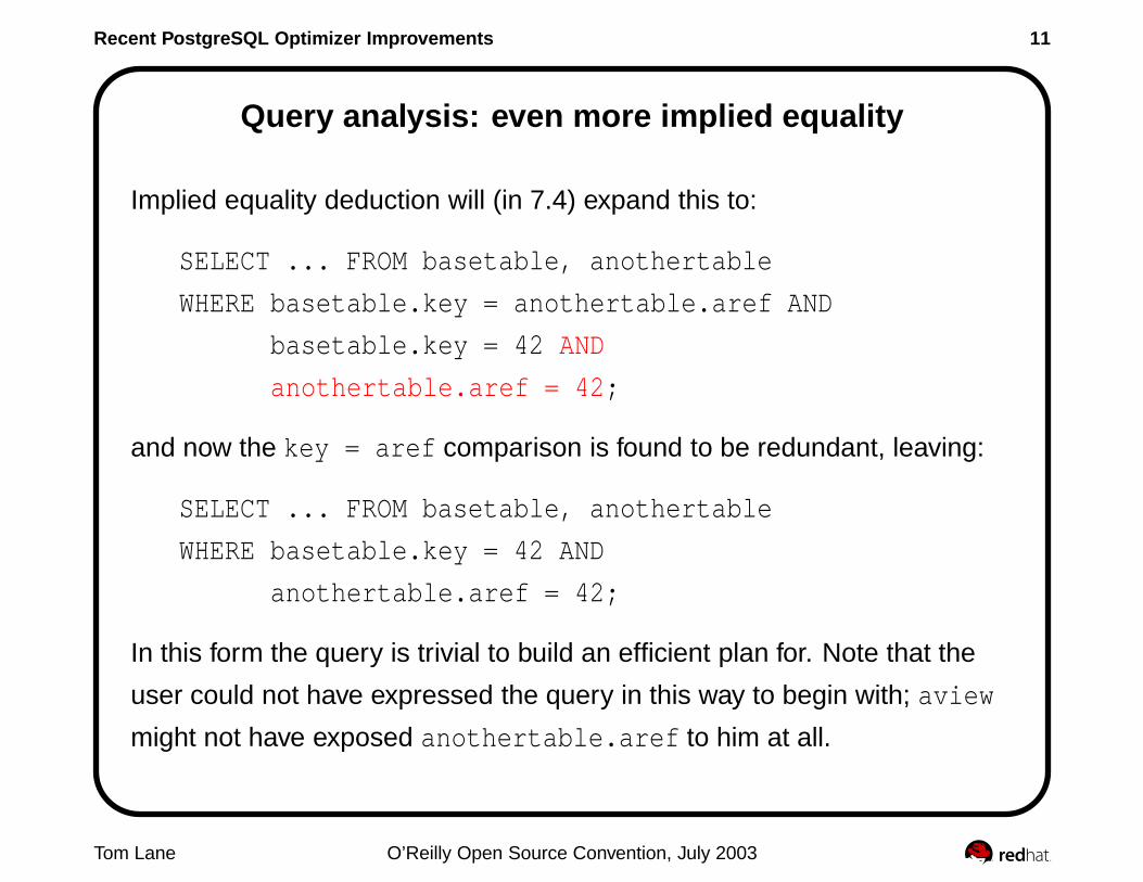
Query analysis: even more implied equality

Implied equality deduction will (in 7.4) expand this to:



basetable.key = 42 AND

anothertable.aref = 42;

and now the key = aref comparison is found to be redundant, leaving:


WHERE basetable.key = 42 AND

anothertable.aref = 42;

In this form the query is trivial to build an efficient plan for. Note that the

user could not have expressed the query in this way to begin with; aview

might not have exposed anothertable.aref to him at all.



Query analysis: distribution of WHERE clauses

Next we attach WHERE clauses to the lowest level at which they can be

evaluated. A clause mentioning just a single table (a.x = 42) is attached

to that table. It will get used when we prepare scan plans for that table.

Join clauses (a.x = b.y) are attached to data structures representing the

sets of tables they mention; they’ll be used when we form a join including

all the tables mentioned.

If we have a WHERE clause that mentions only outputs of a sub-SELECT

(one that’s not been flattened), we try to push it down inside the

sub-SELECT. There are semantic restrictions on whether we can do this

without changing the results, though. 7.4 analyzes the situation more

carefully than prior releases and is able to push down such clauses in

more cases.



The main planning process

After all the preparatory work is done, we generate possible plans and

estimate costs.

First, generate possible scan plans for each individual table: simple

sequential scan is always possible, as well as index scans using each of

the indexes that are relevant to the query. Estimate execution cost for

each.

If there’s only one table, we’re done — just take the cheapest plan.

If there’s more than one table, generate join plans for each pair of tables.

We can do simple nestloop, nestloop with inner index scan, merge join, or

hash join. Merge join needs sorted inputs, so there are multiple

possibilities depending on whether we perform explicit sort steps or use

presorted inputs (for instance, the result of an index scan is already

sorted, if it’s a btree index).



Types of join plans

Nested Loop

aag

Table 2

aag

aar

aai

aay aag

aas

aar

aaa

aay

aai

Table 1

Nested loop with inner index scan uses an index on Table 2 to fetch just

the rows matching the current Table 1 row.



Types of join plans

Merge JoinSorted

Sorted

Table 2

aab

aac

aad

aaa

aab

aab

aaf

aaf

aac

aae

Table 1

aaa

Hash Join

Hashed

Table 1

aar

aak

aay aaraam

aao aaw

Table 2

aay

aag

aas

aak



The main planning process, continued

Next (if there’s at least three tables) look for ways to join pairs of tables

to individual tables to make three-way joined relations, using the cheapest

pairwise joins we found before.

For example, given

SELECT ... FROM tab1, tab2, tab3

WHERE tab1.col1 = tab2.col2 AND tab1.col3 = tab3.col4;

the first pass generates sequential and index scan plans for each of tab1,

tab2, tab3 separately. The second pass generates plans that join tab1

and tab2, as well as plans that join tab1 and tab3. (We could also

consider plans that join tab2 and tab3, but this avenue is rejected

because there is no WHERE clause that constrains that join, so we’d have

to generate the entire cross-product of those two tables.) Finally, the third

pass generates plans that combine tab3 with the join of tab1 and tab2,

and also plans that combine tab2 with the join of tab1 and tab3.



The main planning process, continued

Any of these sequences might be the cheapest way to compute the result,

depending on factors such as the sizes of the tables, the constraints

specified in the query’s WHERE clause, and the available indexes.

If we have more tables, we next look for ways to make four-way joins,

five-way joins, etc, until we have joined all the tables in the query. Each

pass uses the results of prior passes.

Once we have the best plans for the complete join set, we are almost

done. We just add on any additional steps needed for grouping,

aggregation, or sorting (if specified by the query), and we’re done.



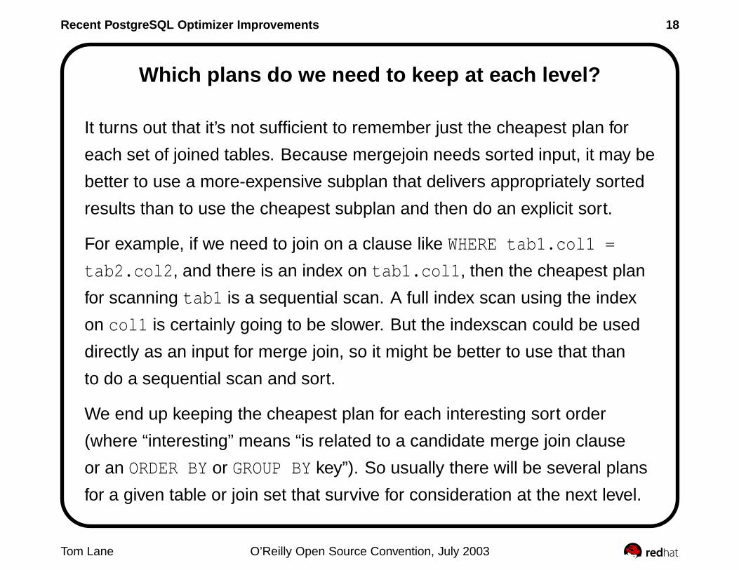
Which plans do we need to keep at each level?

It turns out that it’s not sufficient to remember just the cheapest plan for

each set of joined tables. Because mergejoin needs sorted input, it may be

better to use a more-expensive subplan that delivers appropriately sorted

results than to use the cheapest subplan and then do an explicit sort.

For example, if we need to join on a clause like WHERE tab1.col1 =

tab2.col2, and there is an index on tab1.col1, then the cheapest plan

for scanning tab1 is a sequential scan. A full index scan using the index

on col1 is certainly going to be slower. But the indexscan could be used

directly as an input for merge join, so it might be better to use that than

to do a sequential scan and sort.

We end up keeping the cheapest plan for each interesting sort order

(where “interesting” means “is related to a candidate merge join clause

or an ORDER BY or GROUP BY key”). So usually there will be several plans

for a given table or join set that survive for consideration at the next level.



Better implementation of WHERE foo IN (SELECT . . . )

We used to implement IN (SELECT ...) in the crudest way possible:

each time the value of the condition is needed (possibly once for every row

of the outer query), run the sub-SELECT to see if it produces a row

matching the left-hand side. This is essentially a nestloop join, and it’s

really slow if either the outer query or the sub-SELECT has a lot of rows.

Some people hand-optimize IN into EXISTS:

SELECT ... WHERE col IN (SELECT subcol FROM subtab);

becomes

SELECT ... WHERE

EXISTS (SELECT * FROM subtab WHERE subcol = col);

This still is a nestloop — but if subtab.subcol is indexed, you can at

least make it be a nestloop with inner indexscan.



Better implementation of WHERE foo IN (SELECT . . . )

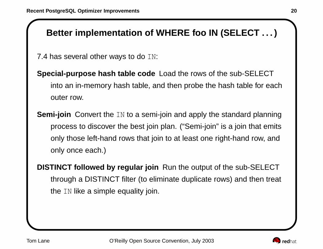
7.4 has several other ways to do IN:

Special-purpose hash table code Load the rows of the sub-SELECT

into an in-memory hash table, and then probe the hash table for each

outer row.

Semi-join Convert the IN to a semi-join and apply the standard planning

process to discover the best join plan. (“Semi-join” is a join that emits

only those left-hand rows that join to at least one right-hand row, and

only once each.)

DISTINCT followed by regular join Run the output of the sub-SELECT

through a DISTINCT filter (to eliminate duplicate rows) and then treat

the IN like a simple equality join.



Better IN (SELECT . . . ): special-purpose hash table

The nasty thing about IN is that the SQL spec dictates that certain cases

involving NULLs in the sub-SELECT result should cause the IN to yield

“unknown” (NULL) rather than “false” when it’s unable to find matching

rows. An ordinary hash join can’t handle this, especially not for a

multi-column IN where rows may be only partly NULL.

By making special entries for rows that are wholly or partly NULL,

we were able to make the special-purpose hash table code produce fully

spec-compliant results for IN. Therefore, we can also use this code for

NOT IN and for cases where the IN operator is nested inside other

boolean operations.

A limitation is that the hash table will perform badly, or even fail outright,

if the sub-SELECT produces more rows than will fit in memory.



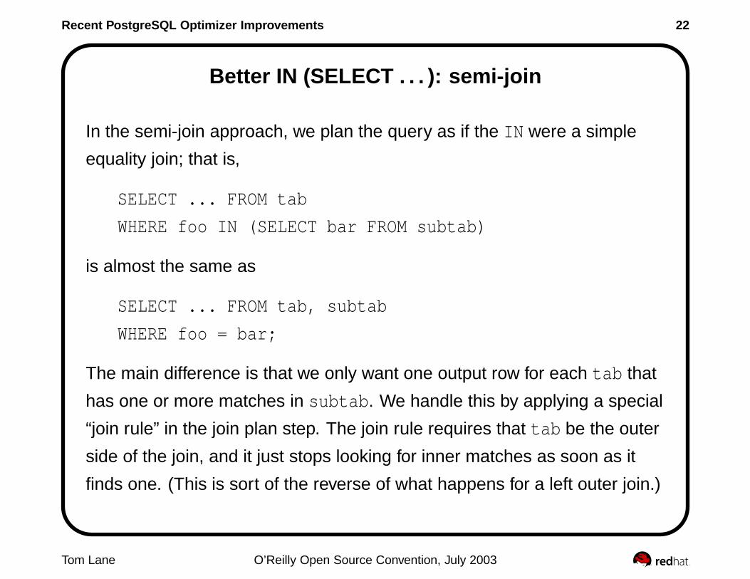
Better IN (SELECT . . . ): semi-join

In the semi-join approach, we plan the query as if the IN were a simple

equality join; that is,

SELECT ... FROM tab

WHERE foo IN (SELECT bar FROM subtab)

is almost the same as

SELECT ... FROM tab, subtab

WHERE foo = bar;

The main difference is that we only want one output row for each tab that

has one or more matches in subtab. We handle this by applying a special

“join rule” in the join plan step. The join rule requires that tab be the outer

side of the join, and it just stops looking for inner matches as soon as it

finds one. (This is sort of the reverse of what happens for a left outer join.)



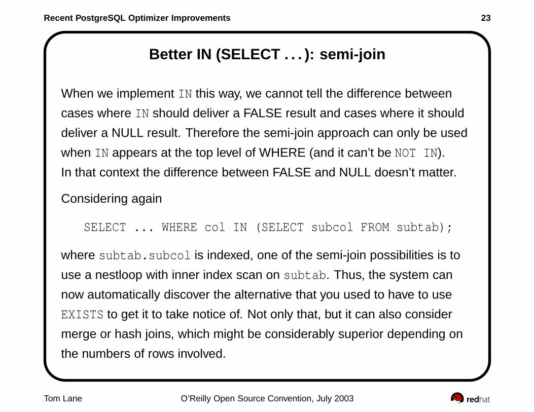
Better IN (SELECT . . . ): semi-join

When we implement IN this way, we cannot tell the difference between

cases where IN should deliver a FALSE result and cases where it should

deliver a NULL result. Therefore the semi-join approach can only be used

when IN appears at the top level of WHERE (and it can’t be NOT IN).

In that context the difference between FALSE and NULL doesn’t matter.

Considering again

SELECT ... WHERE col IN (SELECT subcol FROM subtab);

where subtab.subcol is indexed, one of the semi-join possibilities is to

use a nestloop with inner index scan on subtab. Thus, the system can

now automatically discover the alternative that you used to have to use

EXISTS to get it to take notice of. Not only that, but it can also consider

merge or hash joins, which might be considerably superior depending on

the numbers of rows involved.



Better IN (SELECT . . . ): DISTINCT followed by join

If we eliminate duplicate rows from the result of the sub-SELECT, then we

can just join it to the outer query with a regular equality join — we’ve

ensured there can’t be multiple output rows for a single outer-query row.

Again, this only works at the top level of WHERE. Its advantage over the

semi-join way is that the distinct-ified sub-SELECT can be either the inner

side or the outer side of the resulting join plan.

Consider

SELECT * FROM big table

WHERE key IN (SELECT id FROM small table);

If big table.key is indexed, then it’s probably going to be best to change

the sub-SELECT to SELECT DISTINCT and use the result as the outer

side of a nestloop with inner index scan. This is the only implementation

that can avoid reading all the rows of big table.



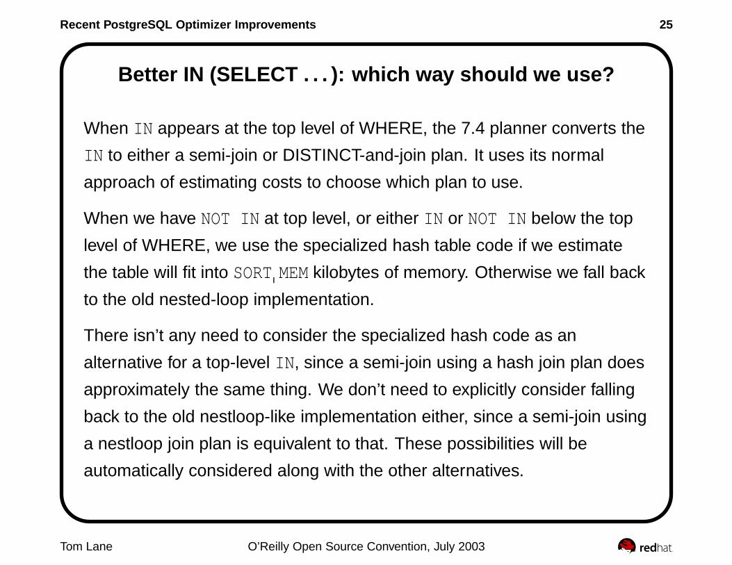
Better IN (SELECT . . . ): which way should we use?

When IN appears at the top level of WHERE, the 7.4 planner converts the

IN to either a semi-join or DISTINCT-and-join plan. It uses its normal

approach of estimating costs to choose which plan to use.

When we have NOT IN at top level, or either IN or NOT IN below the top

level of WHERE, we use the specialized hash table code if we estimate

the table will fit into SORT MEM kilobytes of memory. Otherwise we fall back

to the old nested-loop implementation.

There isn’t any need to consider the specialized hash code as an

alternative for a top-level IN, since a semi-join using a hash join plan does

approximately the same thing. We don’t need to explicitly consider falling

back to the old nestloop-like implementation either, since a semi-join using

a nestloop join plan is equivalent to that. These possibilities will be

automatically considered along with the other alternatives.



Hash-based grouping and grouped aggregation

In 7.3 and before, if you write GROUP BY foo, the implementation always

involves scanning the input in order by foo (via either an explicit sort or

an indexscan). Then group boundaries are detected by comparing the foo

column or columns in successive rows. If we are aggregating, we run the

aggregate accumulation functions on each row as it arrives, then emit

results when the end of a group is detected.

In 7.4, there is another alternative, which is to load the incoming data into

an in-memory hash table indexed by the grouping columns. After we have

read all the input data, we traverse the hash table and emit one result row

for each hash entry; that is, one result for each group.



Hash-based grouping and grouped aggregation

If we are aggregating, we still run the accumulation functions on each row

as it arrives. The hash table entry for each group has to hold the transient

state for each aggregate. So this way is more memory-intensive than the

old way, but as long as there are not too many groups, it’s not a problem.

The big advantage of the hash-based approach is that we don’t have to

pre-sort the input. A disadvantage is that the output will appear in no

particular order. So if you asked for GROUP BY foo ORDER BY foo,

we have to do an explicit sort of the output instead. This can still be a big

win though, since there are likely to be many fewer output rows than input

rows.

The planner chooses between these two approaches in its usual way:

estimate the costs of both and pick the cheaper one. It also checks

whether the hash table is expected to fit in SORT MEM kilobytes — if not,

it won’t use hashing.



Merge and hash joins on expressions

The merge and hash join methods were formerly considered only for join

clauses that equated two simple variables (a.x = b.y). Now they are

considered for join clauses that equate any expressions over different sets

of tables.

For example,

SELECT * FROM a, b WHERE a.foo = b.bar + 1;

is now a candidate for merge or hash joining, whereas before 7.4 it would

always have been done as a brute-force nestloop join.

Also, a hash join can use multiple hash keys rather than only one.



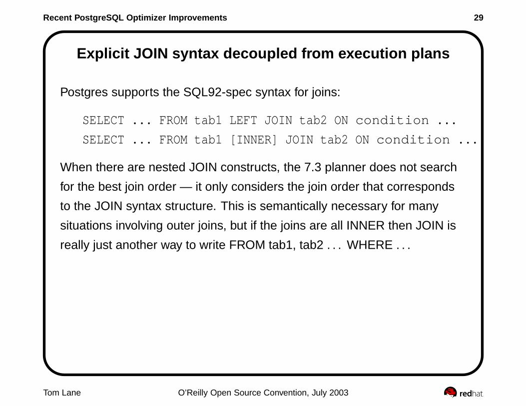
Explicit JOIN syntax decoupled from execution plans

Postgres supports the SQL92-spec syntax for joins:

SELECT ... FROM tab1 LEFT JOIN tab2 ON condition ...

SELECT ... FROM tab1 [INNER] JOIN tab2 ON condition ...

When there are nested JOIN constructs, the 7.3 planner does not search

for the best join order — it only considers the join order that corresponds

to the JOIN syntax structure. This is semantically necessary for many

situations involving outer joins, but if the joins are all INNER then JOIN is

really just another way to write FROM tab1, tab2 . . . WHERE . . .



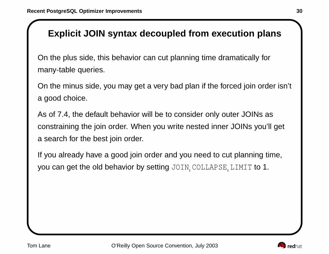
Explicit JOIN syntax decoupled from execution plans

On the plus side, this behavior can cut planning time dramatically for

many-table queries.

On the minus side, you may get a very bad plan if the forced join order isn’t

a good choice.

As of 7.4, the default behavior will be to consider only outer JOINs as

constraining the join order. When you write nested inner JOINs you’ll get

a search for the best join order.

If you already have a good join order and you need to cut planning time,

you can get the old behavior by setting JOIN COLLAPSE LIMIT to 1.



A success story

A few months ago, the Ars Digita guys (who now work at Red Hat)

came to me for help with porting their ACS system to PostgreSQL. They

had problems with four queries that were used in displaying web pages in

ACS. These queries each took several seconds to execute in PostgreSQL,

making the performance unacceptable. The same queries ran fine in

Oracle.

But . . . they were testing on PostgreSQL 7.2.

I was able to tell them that all their problems were already solved.



A success story

Measured runtimes for the problem queries (same data, same machine):

PG 7.2 PG 7.3 As of 14-Mar-03

Query 1 4560.62 msec 4461.84 msec 213.14 msec

Win from: searching for good join order instead of following JOIN structure


Win from: pushing down WHERE clauses into UNION (already done in 7.3)


7.3 win from: evaluating IN last among clauses attached to same plan node

7.4 win from: converting IN to special-purpose hash table


Win from: searching for good join order



A success story

Mind you, these are pretty ugly queries — here’s the first one:

select *

from (select *

from vc objects join acs objects

on (vc objects.object id=acs objects.object id)

join cms items

on (vc objects.object id=cms items.item id)) results

where (cms items ancestors<=’19056/’)

and (cms items ancestors=substr(’19056/’,1,

length(cms items ancestors)))

order by cms items ancestors;

But they are real-world examples.



Summary

There’s lots of good new stuff coming in 7.4.

Since internal hash tables are options in many more places than before,

and each one can use up to SORT MEM kilobytes, it’s more important than

ever to make sure you set that parameter intelligently. Too small will

handicap performance by preventing hash-based plans from being

considered, but too large can drive your system into swap hell.

If you’ve hand-optimized IN queries into EXISTS queries, you might want

to think about switching back. Under 7.4 using EXISTS could be a

de-optimization, because it constrains the planner to use only one of the

types of plans it would consider if you used IN.


recent postgresql optimizer improvements 1

Documents