recent advances on bootstrap methods for … 2009/bootstrap_spectral...recent advances on bootstrap...
TRANSCRIPT
The Bootstrap in Signal Processing
Abdelhak M Zoubir
Recent Advances on Bootstrap Methods forSpectral Analysis
Abdelhak M Zoubir
S i g n a l P r o c e s s i n g G r o u p
Signal Processing Group
Technische Universitat Darmstadt
E-Mail: [email protected]
URL: www.spg.tu-darmstadt.deMay 10, 2010 | SPG TUD | c© A.M. Zoubir | 1 SPG

Motivation
◮ Spectral analysis is an important tool for science and engineering and has
been a subject of study since the 19th Century [Stokes (1879), Schuster
(1894)].◮ There are three principal reasons for using spectral analysis:
◮ to provide useful descriptive statistics,◮ as a diagnostic tool to indicate which further analyses might be relevant,◮ to check postulated theoretical models.
◮ Frequency analysis is now firmly involved in various areas of electrical
engineering, such as communications, radar and sonar.◮ Statistical inference for spectra and functions of spectra such coherence and
transfer functions is fundamental in these areas.◮ Most techniques for statistical inference rely on assumptions [Rosenblatt
(1985), Priestley (1981)], which may not hold in practice.
May 10, 2010 | SPG TUD | c© A.M. Zoubir | 2 SPG

Motivation (Cont’d)
◮ Let Xt , t ∈ Z, be a real-valued strictly stationary process with covariance
function cXX (τ) = E[X0X|τ |], τ ∈ Z, and spectral density
CXX (ω) =1
2π
∞∑
τ=−∞
cXX (τ)e−jωτ , −π < ω ≤ π.
◮ Given the model X1, X2, ... , XT for the observations x1, x2, ... , xT ,
we wish to find:
◮ an estimator CXX (ω) for CXX (ω), and
◮ an 100(1− α)% confidence interval for CXX (ω), for a given α.
May 10, 2010 | SPG TUD | c© A.M. Zoubir | 3 SPG

Motivation (Cont’d)
◮ Define the periodogram of Xt ,
IXX (ω) =1
2πT
∣
∣
∣
∣
∣
T∑
t=1
Xte−jωt
∣
∣
∣
∣
∣
2
, −π < ω ≤ π
◮ and construct the estimator of CXX (ω) by
CXX (ω) =1
T · h
n∑
k=−n
K
(
ω − ωk
h
)
IXX (ωk),
where the kernel K (·) is a known symmetric, non-negative, real-valued
function, h is its bandwidth and n = [T/2].
May 10, 2010 | SPG TUD | c© A.M. Zoubir | 4 SPG

Motivation (Cont’d)
0 0.2 0.4 0.6 0.8 10
5
10
15
20
25
ω/π
Spe
ctra
l Den
sity
Spectral density of an AR(6) process (—), the periodogram (...) and the spectral density
estimate (-.-) for T = 256, h = 0.1 and the Bartlett-Priestley kernel K(·).
May 10, 2010 | SPG TUD | c© A.M. Zoubir | 5 SPG

Motivation (Cont’d)
◮ Under some regularity conditions, we have asymptotically for T → ∞,
CXX (ω) ∼ CXX (ω)
4m + 2χ2
4m+2,
m = ⌊(hT − 1)/2⌋ .
◮ An 100(1 − α)% confidence interval for CXX (ω) is found as,
(4m + 2)CXX (ω)
χ24m+2(1 − α
2 )< CXX (ω) <
(4m + 2)CXX (ω)
χ24m+2(
α2 )
,
where χ2ν(α) is such that Prob[χ2
ν < χ2ν(α)] = α [Brillinger (1981)].
May 10, 2010 | SPG TUD | c© A.M. Zoubir | 6 SPG

Motivation (Cont’d)
0 20 40 60 80 100 1200
0.2
0.4
0.6
0.8
1
1.2
frequency [k]
spec
tral
den
sity
0 20 40 60 80 100 1200
0.5
1
1.5
2
2.5
3
3.5
4
frequency [k]
spec
tral
den
sity
95% confidence interval for CXX (ω) of the Gaussian process
Xt = 0.5Xt−1 − 0.6Xt−2 + 0.3Xt−3 − 0.4Xt−4 + 0.2Xt−5 + εt (left) and
Yt = Yt−1 − 0.7Yt−2 − 0.4Yt−3 + 0.6Yt−4 − 0.5Yt−5 + ζt (right), where ζt are identically
and independently uniformly distributed on U [−π, π). The true CXX (ω) (—) and an
estimate based on T = 256 (...) are given.
May 10, 2010 | SPG TUD | c© A.M. Zoubir | 7 SPG
Limitations
◮ We assumed a large T so that CXX (ω1), ... , CXX (ωM) are independently and
identically distributed as χ2 ramdom variates.◮ Asymptotic approaches are often inapplicable:
◮ real-time applications do not always permit collection of long data segments
[Bendat & Piersol (2000)], or
◮ we restrict the sample size to be small for the (quasi) stationarity assumption.
◮ analytical solutions for the finite sample case are often tedious or impossible.◮ Bootstrap techniques are the alternative to asymptotic theory for short data
segments and perform usually better under weaker assumptions [Efron
(1979), Hall (1992), Efron & Tibshirani (1993), Davison & Hinkley (2006)].
May 10, 2010 | SPG TUD | c© A.M. Zoubir | 8 SPG

Contents
◮ Introduction
◮ What can I use the bootstrap for?◮ How does the bootstrap work?◮ Why does the bootstrap work?◮ History of the bootstrap
◮ The independent data bootstrap
◮ An example for independent data◮ An example of independent data bootstrap for dependent data
◮ The bootstrap principle for dependent data
◮ The moving blocks bootstrap◮ Other block bootstrap methods
May 10, 2010 | SPG TUD | c© A.M. Zoubir | 9 SPG

Contents
◮ Frequency domain bootstrap methods for dependent data
◮ The multiplicative regression approach◮ The local bootstrap for periodogram statistics◮ The autoregressive-aided periodogram bootstrap
◮ Two real-life examples of the bootstrap
◮ Confidence bounds for spectra of combustion engine knock data◮ Micro-Doppler analysis
◮ Concluding remarks
May 10, 2010 | SPG TUD | c© A.M. Zoubir | 10 SPG

Introduction (Cont’d)
◮ The term bootstrap is often associated with The Baron von Munchhausen.
Courtesy of Prof. Dr. Karl Heinrich Hofmann, TU Darmstadt and Head of Group Algebra, Geometry and Functional Analysis
May 10, 2010 | SPG TUD | c© A.M. Zoubir | 11 SPG

Introduction (Cont’d)
◮ This analogy may suggest that the bootstrap is able to perform the
impossible.
◮ The bootstrap is not a magic technique that provides a panacea for all
statistical inference problems!
◮ The bootstrap is a powerful tool that can substitute tedious or often
impossible theoretical derivations with computational calculations.
◮ There are situations where the bootstrap fails and care is required [Young
(1994)].
May 10, 2010 | SPG TUD | c© A.M. Zoubir | 12 SPG

What can I use the bootstrap for?
◮ The bootstrap is a computational tool for statistical inference.
◮ It can be used for:
◮ Estimation of statistical characteristics such as bias, variance, distribution
function of estimators and thus confidence intervals.◮ Hypothesis tests, for example for signal detection, and◮ model selection.
◮ When can I use the bootstrap?
When I know little about the statistics of the data and/or I have only
a few data so that asymptotic theory does not hold.
May 10, 2010 | SPG TUD | c© A.M. Zoubir | 13 SPG

The Bootstrap Idea
Model
Unknown EstimatedProbability
Model
^
REAL WORLD
21X=(x , x , ..., x )F
Probability
θ
n
^
F^ x*=(x* , x* , ..., x* )1 2
θ*=s( *)x
Observed Data Bootstrap Sample
x=s( )Bootstrap replicationStatistic of interest
BOOTSTRAP WORLD
n
Basic idea: simulate the probability mechanism of the real world by substituting the
unknowns with estimates derived from the data.
May 10, 2010 | SPG TUD | c© A.M. Zoubir | 14 SPG

Why Does the Bootstrap Work?
◮ Let the distribution of T admit an Edgeworth expansion,
G(x) = P(T ≤ x) = Φ(x) + n−1/2q(x)φ(x) + O(n−1),
where q is an even quadratic polynomial and Φ,φ are standard normal
distribution and density function, respectively.◮ The bootstrap estimate of G admits an analogous expansion
G(x) = P(T ∗ ≤ x |X ) = Φ(x) + n−1/2q(x)φ(x) + Op(n−1),
where q is obtained from q on replacing unknowns by bootstrap estimates.◮ Because q − q = Op(n
−1/2),
G(x) − G(x) = P(T ∗ ≤ x |X ) − P(T ≤ x) = Op(n−1/2)
Thus, the bootstrap approximation is in error by n−1 while the normal
approximation Φ is in error by n−1/2 .
May 10, 2010 | SPG TUD | c© A.M. Zoubir | 15 SPG
A Brief History Recount
◮ It was by marrying the power of Monte Carlo approximation with an
exceptionally broad view of the sort of problem that bootstrap methods
might solve, that [Efron (1979)] famously vaulted earlier resampling ideas out
of the arena of sampling methods and into the realm of a universal statistical
methodology.
◮ Arguably, the prehistory of the bootstrap encompasses pre-1979
developments of Monte Carlo methods for sampling.
◮ Important aspects of bootstrap roots lie in methods for spatial sampling in
India in the 1920’s [Hubback (1946), Mahalanobis (1946)], even before
Quenouille’s and Tukey’s work on the jackknife [Quenouille (1949, 1956),
Tukey (1958)].
May 10, 2010 | SPG TUD | c© A.M. Zoubir | 16 SPG

The independent data bootstrap
May 10, 2010 | SPG TUD | c© A.M. Zoubir | 17 SPG
The Bootstrap for independent Data
Step 1. Conduct the experiment to obtain the random sample
X = {X1, X2, ... , Xn} and find the estimator θ from X .
Step 2. Construct the empirical distribution Fθ, which puts equal mass 1/n
at each observation X1 = x1, X2 = x2, ... , Xn = xn.
Step 3. From the selected Fθ, draw a sample X ∗ = {X ∗1 , X ∗
2 , ... , X ∗n },
called the bootstrap (re)sample.
Step 4. Approximate the distribution of θ by the distribution of θ∗ derived
from X ∗.
May 10, 2010 | SPG TUD | c© A.M. Zoubir | 18 SPG

Implementation of the Bootstrap Procedure
Measured Data
Conduct
Experiment- - Compute
Statistic-
xθ(x)
?Resample
Bootstrap Data
- - Compute
Statistic-
x∗1
θ∗1
- - Compute
Statistic-
x∗2
θ∗2
.
.
.
.
.
.
- - Compute
Statistic-
x∗B
θ∗B
Generate
EDF,
FΘ
(θ)
-
-θ
6FΘ
(θ)
Algorithm to compute the approximative distribution function of the estimator θ.
May 10, 2010 | SPG TUD | c© A.M. Zoubir | 19 SPG

Resampling i.i.d. Data
◮ A resample X ∗ = {X ∗1 , X ∗
2 , ... , X ∗n } is an unordered collection of n sample
points drawn randomly from X with replacement, so that each X ∗i has
probability n−1 of being equal to any one of the Xj ’s. In other terms,
P (X ∗i = Xj | X ) = n−1 , 1 ≤ i , j ≤ n.
◮ That is, the X ∗i ’s are independent and identically distributed, conditional on
the random sample X , with this distribution [Hall (1992)].
This means that X ∗ is likely to contain repeats. As an example, consider n = 4
and the collection X ∗ = {0.5,−3.7,−3.7, 2.8} which should not be mistaken for
the set {0.5,−3.7, 2.8} because the bootstrap sample has one repeat. Also, X ∗ is
the same as {0.5,−3.7, 2.8,−3.7}, {−3.7, 0.5, 2.8,−3.7}, etc. because the order
of elements in the resample plays no role [Hall (1992), Efron & Tibshirani (1993)].
May 10, 2010 | SPG TUD | c© A.M. Zoubir | 20 SPG
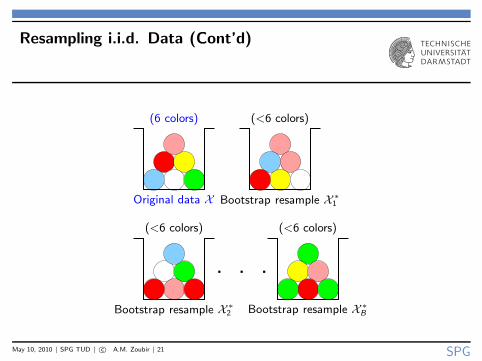
Resampling i.i.d. Data (Cont’d)
(6 colors) (<6 colors)
(<6 colors) (<6 colors)
Original data X Bootstrap resample X ∗
1
Bootstrap resample X ∗
2 Bootstrap resample X ∗
B
. . .
May 10, 2010 | SPG TUD | c© A.M. Zoubir | 21 SPG
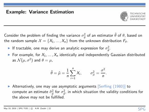
Example: Variance Estimation
Consider the problem of finding the variance σ2θ
of an estimator θ of θ, based on
the random sample X = {X1, ... , Xn} from the unknown distribution Fθ.
◮ If tractable, one may derive an analytic expression for σ2θ.
◮ For example, for X1, ... , Xn identically and independently Gaussian distributed
as N (µ, σ2) and θ = µ,
θ = µ =1
n
n∑
i=1
Xi , σ2µ =
σ2
n.
◮ Alternatively, one may use asymptotic arguments [Serfling (1980)] to
compute an estimate σ2θ
for σ2θ, in which situation the validity conditions for
the above may not be fulfilled.
May 10, 2010 | SPG TUD | c© A.M. Zoubir | 22 SPG

Example: Variance Estimation of µ
X = {X1, ... , Xn}
X ∗1 X ∗
2 X ∗B
µ∗1 µ∗
2 µ∗B
σ∗2µ = 1
B−1
∑B
b=1
(
µ∗b − 1
B
∑B
b=1 µ∗b
)2
Observations
Resamples
Bootstrap statistics
Variance estimation
May 10, 2010 | SPG TUD | c© A.M. Zoubir | 23 SPG

The independent data bootstrap
for dependent data
May 10, 2010 | SPG TUD | c© A.M. Zoubir | 24 SPG

The Independent Data Bootstrap for Depen-
dent Data
◮ The assumption of i.i.d. data can break down in practice either because the
data is not independent or because it is not identically distributed, or both.
◮ We can still invoke the bootstrap principle if we knew the model that
generated the data [Efron & Tibshirani (1993), Bose (1988), Kreiß & Franke
(1992), Paparoditis (1996), Zoubir (1993)].
◮ For example, a way to relax the i.i.d. assumption is to assume that the data
is identically distributed but not independent such as in autoregressive (AR)
models.
May 10, 2010 | SPG TUD | c© A.M. Zoubir | 25 SPG

An Example: Variance Estimation
Assume T observations xt , t = 0, ... , T − 1, from
Xt + a · Xt−1 = Zt ,
where Zt is i.i.d. noise with E[Zt ] = 0, cZZ (u) = σ2Z δ(u) and a such that |a| < 1.
Goal: Estimate the variance of a.
An estimate for the variance of a exists asymptotically and for Zt Gaussian:
◮ Detrend the data and fit the AR(1) model to xt , t = 0, ... , T − 1.
◮ With cxx(u) = 1/T∑T−|u|−1
t=0 xtxt+|u| for 0 ≤ |u| ≤ T − 1, calculate the
Maximum Likelihood Estimate (MLE) of a, a = −cxx(1)/cxx(0), which has
approximate variance σ2a = (1 − a2)/T .
May 10, 2010 | SPG TUD | c© A.M. Zoubir | 26 SPG
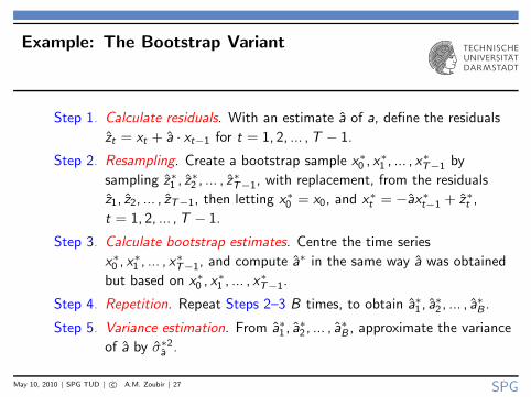
Example: The Bootstrap Variant
Step 1. Calculate residuals. With an estimate a of a, define the residuals
zt = xt + a · xt−1 for t = 1, 2, ... ,T − 1.
Step 2. Resampling. Create a bootstrap sample x∗0 , x∗
1 , ... , x∗T−1 by
sampling z∗1 , z∗2 , ... , z∗T−1, with replacement, from the residuals
z1, z2, ... , zT−1, then letting x∗0 = x0, and x∗
t = −ax∗t−1 + z∗t ,
t = 1, 2, ... ,T − 1.
Step 3. Calculate bootstrap estimates. Centre the time series
x∗0 , x∗
1 , ... , x∗T−1, and compute a∗ in the same way a was obtained
but based on x∗0 , x∗
1 , ... , x∗T−1.
Step 4. Repetition. Repeat Steps 2–3 B times, to obtain a∗1 , a∗2 , ... , a
∗B .
Step 5. Variance estimation. From a∗1 , a∗2 , ... , a
∗B , approximate the variance
of a by σ∗2a .
May 10, 2010 | SPG TUD | c© A.M. Zoubir | 27 SPG

Example (Cont’d)
−0.8 −0.7 −0.6 −0.5 −0.4 −0.3 −0.2 −0.10
1
2
3
4
5
6
Bootstrap estimates
Den
sity
func
tion
Histogram of a∗
1 , a∗
2 , ... , a∗
1000 for a = −0.6, T = 128 and Zt Gaussian. The MLE for a is
a = −0.6351 and σa = 0.0707. The bootstrap estimate is σ∗
a = 0.0712 as compared to
σa = 0.0694 based on 1000 Monte Carlo simulations.
May 10, 2010 | SPG TUD | c© A.M. Zoubir | 28 SPG

The Dependent Data Bootstrap (Cont’d)
◮ If no plausible model such as AR is available for the probability mechanism
generating stationary observations, we could make the assumption of weak
dependence.
◮ Strong mixing processes, i.e., loosely speaking, processes for which
observations far apart (in time) are almost independent [Rosenblatt (1985)],
for example, satisfy the weak dependence condition.
◮ The moving blocks bootstrap [Kunsch (1989), Liu & Singh (1992), Politis &
Romano (1992,1994)] has been proposed for bootstrapping weakly dependent
data.
May 10, 2010 | SPG TUD | c© A.M. Zoubir | 29 SPG

The Moving Blocks Bootstrap
0 10 20 30 40 50 60 70 80 90 100−5
0
5
Sample number
Am
plit
ud
e
Bootstrap Data0 10 20 30 40 50 60 70 80 90 100
−5
0
5
Am
plit
ud
e
Resampled Blocks
54321
0 10 20 30 40 50 60 70 80 90 100−5
0
5
Am
plit
ud
e
Observed Data
12 345
Randomly select blocks of the original data (top) and concatenate them together
(centre) to form a resample (bottom). Here, the block size is l = 20 and n = 100.
May 10, 2010 | SPG TUD | c© A.M. Zoubir | 30 SPG

Other Block Bootstrap Methods
◮ The circular block bootstrap [Politis & Romano (1992), Shao & Yu (1993)]
allows blocks which start at the end of the data and wrap around to the start.
◮ The blocks of blocks bootstrap [Politis et al. (1992)] uses two levels of
blocking to estimate confidence bands for spectra and cross-spectra.
◮ The stationary bootstrap [Politis & Romano (1994)] allows blocks to be of
random lengths instead of a fixed length.
◮ The tapered block bootstrap [Paparoditis & Politis (2001)] assigns different
weights to the data points according to their position within their block. This
results in a bias correction of Kunsch’s method while preserving asymptotic
validity.
May 10, 2010 | SPG TUD | c© A.M. Zoubir | 31 SPG
Frequency domain bootstrap
methods for dependent data
May 10, 2010 | SPG TUD | c© A.M. Zoubir | 32 SPG

Bootstrapping Spectral Densities
◮ Confidence interval estimation (or hypothesis testing) for spectral densities is
encountered in numerous real-life applications, e.g., car engine monitoring.
◮ Two approaches to bootstrapping spectral densities:
◮ Use a time domain approach (block bootstrap) to bootstrap time series and
estimate bootstrap spectral density estimates from the time series replicae, or◮ use a technique that applies directly in the frequency domain.
◮ Bootstrap time series not always mimic the (complicated) dependence
structure of the underlying process.
◮ Frequency domain bootstrap methods do not require to first generate time
series replicae to get periodogram resamples.
May 10, 2010 | SPG TUD | c© A.M. Zoubir | 33 SPG

Frequency Domain Bootstrap (Cont’d)
◮ Assume Xt , t ∈ Z to be a real-valued strictly stationary process, with
representation Xt =∑∞
τ=−∞ hτEt−τ , t ∈ Z.◮ Given X1, ... , XT , define the periodogram by
IXX (ω) =1
2πT
∣
∣
∣
∣
∣
T∑
t=1
Xte−jωt
∣
∣
∣
∣
∣
2
, −π ≤ ω ≤ π
◮ and construct the estimator of CXX (ω) by
CXX (ω) =1
T · h
n∑
k=−n
K
(
ω − ωk
h
)
IXX (ωk),
where the kernel K (·) is a known symmetric, non-negative, real-valued
function, h is its bandwidth and n = [T/2].
May 10, 2010 | SPG TUD | c© A.M. Zoubir | 34 SPG
Frequency Domain Bootstrap (Cont’d)
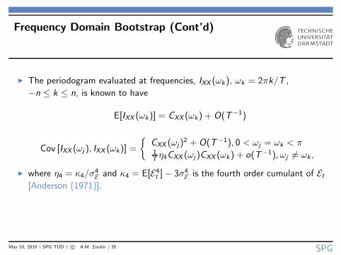
◮ The periodogram evaluated at frequencies, IXX (ωk), ωk = 2πk/T ,
−n ≤ k ≤ n, is known to have
E[IXX (ωk)] = CXX (ωk) + O(T−1)
Cov [IXX (ωj), IXX (ωk)] =
{
CXX (ωj)2 + O(T−1), 0 < ωj = ωk < π
1T
η4CXX (ωj)CXX (ωk) + o(T−1), ωj 6= ωk ,
◮ where η4 = κ4/σ4E and κ4 = E[E4
t ] − 3σ4E is the fourth order cumulant of Et
[Anderson (1971)].
May 10, 2010 | SPG TUD | c© A.M. Zoubir | 35 SPG

The Residual Based Bootstrap
◮ The residual based method [Franke & Hardle (1992)] is based on the
multiplicative regression
IXX (ωk) = CXX (ωk)IEE(ωk)
2πσ2E
+ RT (ωk),
IEE(ωk) =1
2πT
∣
∣
∣
∣
∣
T∑
t=1
Ete−jωk t
∣
∣
∣
∣
∣
2
, ωk =2πk
T, k = 0, ... , n,
◮ with RT (ωk) satisfying maxωk∈[0,π]E[RT (ωk)2] = O(T−1) [Brockwell & Davis
(1991)].
◮ Ignoring RT (ωk) and taking into account the asymptotic independence of
periodogram ordinates, suggests resampling periodograms via mimicking the
behavior of IEE(ωk )/σ2E and replacing CXX by CXX .
May 10, 2010 | SPG TUD | c© A.M. Zoubir | 36 SPG

The Residual Based Bootstrap (Cont’d)
DataMeasured
x
ConductExperiment
BootstrapData
Reconstruct& Estimate
Reconstruct& Estimate
CXX
`
ωk
´
SmoothPeriodogram
Reconstruct& Estimate
Resample
Uk =IXX
`
ωk
´
CXX
`
ωk
´
Confidence
IntervalSort
k = 1, ... , M
FindPeriodogram
C∗(B)XX
`
ωk
´
C∗(2)XX
`
ωk
´
C∗(1)XX
`
ωk
´
, ...
... , C∗(B)XX
`
ωk
´
IXX
`
ωk
´
U∗k,1
U∗k,2
U∗k,B
C∗(1)XX
`
ωk
´
May 10, 2010 | SPG TUD | c© A.M. Zoubir | 37 SPG

The Residual Based Bootstrap (Cont’d)
◮ The residual based method approximates the distribution of
LT (ω) =√
Th(CXX (ω) − CXX (ω))/CXX (ω) through the distribution of
L∗T (ω) =
√Th(C∗
XX (ω) − CXX (ω))/CXX (ω) where
C∗XX (ω) =
1
T · h
n∑
k=−n
K
(
ω − ωk
h
)
I ∗XX (ωk)
◮ Under some regularity conditions (see above and some more on the
estimation of CXX (ω)) [Franke & Hardle (1992), Paparoditis (2002)], we have
d2 (L{LT (ω)} ,L{L∗T (ω) |X1, X2, ... , XT }) → 0 in probability
May 10, 2010 | SPG TUD | c© A.M. Zoubir | 38 SPG

The Local Bootstrap
◮ An alternative method which does not require prior estimation of the spectral
density [Paparoditis & Politis (1999)].
◮ Recall that for large T , IXX (ω) is approximately exponentially distributed
with parameter CXX (ω).
Idea: For CXX (ω) a smooth function of ω, it is expected that the sampling behaviour of
the periodogram at any particular frequency ωs will be similar for periodogram ordinates
corresponding to frequencies in a small neighboorhood of ωs . Thus, periodogram replicae
at ωs can be obtained by locally resampling the periodogram, i.e., by choosing with
replacement between periodogram ordinates corresponding to frequencies ’close’ to ωs .
Validity: Under some regularity conditions [Paparoditis (2002)],
d2
`
L{LT (ω)} ,L˘
L+T (ω) |X1,X2, ... , XT
¯´
→ 0 in probability
May 10, 2010 | SPG TUD | c© A.M. Zoubir | 39 SPG

Limitations
◮ The previous two methods assume independence of the periodogram ordinates
I ∗XX (ω) and I+XX (ω), justified by the asymptotic independence of IXX (ω).
◮ One should take into account the weak dependence structure of the
periodogram ordinates.
◮ One approach is to modify appropriately the above procedures.
◮ Using a non-parametric estimator of η4, Janas & Dahlhaus (1994) modified
I ∗XX (ω) in a way that emulates also the covariance of IXX (ω).
◮ It is problematic to nonparametrically estimate the complicated functional η4
[Dahlhaus & Janas (1996)].
May 10, 2010 | SPG TUD | c© A.M. Zoubir | 40 SPG

Autoregressive-Aided Periodogram Bootstrap
◮ An alternative is the so-called autoregressive-aided periodogram bootstrap
[Kreiss & Paparoditis (2003)], a combination of time domain and frequency
domain resampling [Zoubir (2010)].
Idea: Use a parametric fit in the time domain to generate periodogram ordinates that
imitate the essential features of the data and weak dependence structure of the
periodogram, while a non-parametric kernel based correction in the frequency domain is
applied to catch features not represented by the parametric fit.
May 10, 2010 | SPG TUD | c© A.M. Zoubir | 41 SPG
The AR-Aided Bootstrap (Cont’d)
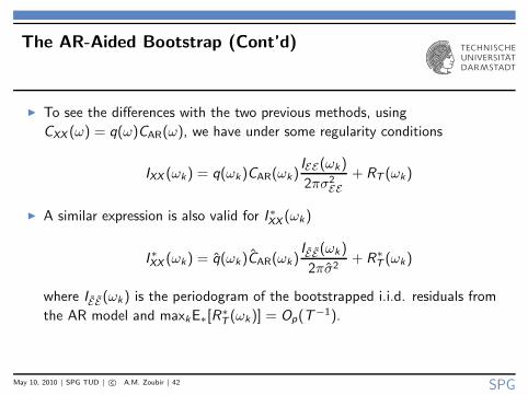
◮ To see the differences with the two previous methods, using
CXX (ω) = q(ω)CAR(ω), we have under some regularity conditions
IXX (ωk) = q(ωk)CAR(ωk)IEE(ωk)
2πσ2EE
+ RT (ωk)
◮ A similar expression is also valid for I ∗XX (ωk)
I ∗XX (ωk) = q(ωk)CAR(ωk)IEE(ωk)
2πσ2+ R∗
T (ωk)
where IEE(ωk) is the periodogram of the bootstrapped i.i.d. residuals from
the AR model and maxkE∗[R∗T (ωk)] = Op(T
−1).
May 10, 2010 | SPG TUD | c© A.M. Zoubir | 42 SPG

A Simulation Example
◮ Consider Xt , where Ut are
independent uniformly distributed
variables on the interval [−2.5, 2.5]
and T = 256
Xt = Xt−1 − 0.7Xt−2 − 0.4Xt−3
+0.6Xt−4 − 0.5Xt−5 + Ut
Estimates of coverage probabilities in [%] of a
nominal 95% confidence interval (1000 MC).
k RSD TBB AR AR-AP
26 86.68 77.98 87.66 88.27
27 85.94 77.55 87.54 87.85
28 85.64 77.77 87.62 87.96
52 84.08 78.48 85.76 87.60
53 83.61 77.80 85.88 87.43
54 84.30 77.88 86.44 87.56
95 86.73 76.74 87.72 90.31
96 87.52 77.41 87.78 90.80
97 87.80 77.98 87.85 91.32
May 10, 2010 | SPG TUD | c© A.M. Zoubir | 43 SPG
Two real-life example
of the bootstrap
May 10, 2010 | SPG TUD | c© A.M. Zoubir | 44 SPG

Confidence Intervals for knock Spectra
◮ Special interest continues to a be reduction of fuel consumption in
combustion engines due to meeting the demands of new legislations on
greenhouse emission.
◮ A means for lowering fuel consumption in spark ignition engines is to increase
the compression ratio. Further increase in compression is limited by the
occurrence of knock.
◮ To attain safe operation at maximum efficiency, engine control systems which
detect knock and adapt spark timing of each cylinder separately have found
special interest.
◮ The data was collected at Robert Bosch GmbH on an engine test bed.
Measurements from a combustion engine running at 3500 rpm under
knocking conditions were recorded and sampled at 100 kHz.
May 10, 2010 | SPG TUD | c© A.M. Zoubir | 45 SPG

Confidence Intervals for knock Spectra
◮ The estimation of confidence intervals is very helpful for the detection of
knock.
◮ There is a well known and established duality between confidence intervals
and hypothesis testing [Lehman (1986)].
◮ if I is a confidence interval for an unknown parameter θ, with coverage
probability α, then a (1 − α)-level test of the null hypothesis H : θ = θ0
against K : θ 6= θ0 is to reject H if θ0 /∈ I.
May 10, 2010 | SPG TUD | c© A.M. Zoubir | 46 SPG
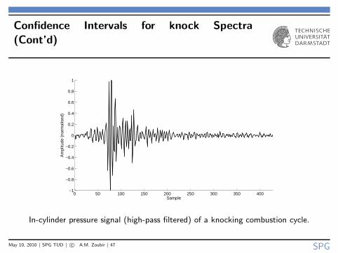
Confidence Intervals for knock Spectra
(Cont’d)
0 50 100 150 200 250 300 350 400−1
−0.8
−0.6
−0.4
−0.2
0
0.2
0.4
0.6
0.8
1
Sample
Am
plitu
de (
norm
alis
ed)
In-cylinder pressure signal (high-pass filtered) of a knocking combustion cycle.
May 10, 2010 | SPG TUD | c© A.M. Zoubir | 47 SPG

Confidence Intervals for knock Spectra
(Cont’d)
0 50 100 150 200 250 300 350 400−1
−0.8
−0.6
−0.4
−0.2
0
0.2
0.4
0.6
0.8
1
Sample
Am
plitu
de (
norm
alis
ed)
Structure-borne sound signal of a knocking combustion cycle.
May 10, 2010 | SPG TUD | c© A.M. Zoubir | 48 SPG

Confidence Intervals for knock Spectra
(Cont’d)
0 5 10 15 20 25 30 35 40 45 50−60
−50
−40
−30
−20
−10
0
Frequency [kHz]
Spe
ctra
l den
sity
(no
rmal
ised
)[dB
]
Spectral density estimates for in-cylinder pressure (solid —) and structure-borne sound
(dashed-dotted -.-) obtained by averaging 594 periodograms.
May 10, 2010 | SPG TUD | c© A.M. Zoubir | 49 SPG

Confidence Intervals for knock Spectra
(Cont’d)
0 5 10 15 20 25 30 35 40 45 50−50
−45
−40
−35
−30
−25
−20
−15
−10
−5
0
Frequency [kHz]
Spe
ctra
l den
sity
(no
rmal
ised
) [d
B]
Estimated 95% confidence interval (dashed line - - -) for the spectral density of
in-cylinder pressure, along with the spectral density estimate for the combustion cycle
above.May 10, 2010 | SPG TUD | c© A.M. Zoubir | 50 SPG

Confidence Intervals for Knock Spectra
(Cont’d)
0 5 10 15 20 25 30 35 40 45 50−70
−60
−50
−40
−30
−20
−10
0
Frequency [kHz]
Spe
ctra
l den
sity
(no
rmal
ised
) [d
B]
Estimated 95% confidence interval for the spectral density of structure-borne sound
(dashed line - –), along with the spectral density estimate for the combustion cycle above
May 10, 2010 | SPG TUD | c© A.M. Zoubir | 51 SPG

Micro-Doppler Analysis
◮ Doppler often arises in engineering applications due to the relative motion of
an object with respect to the measurement system.
◮ If the motion is harmonic, for example due to vibration or rotation, the
resulting signal can be well modeled by an FM process [Huang et al. (1990)].
◮ Estimation of the FM parameters may allow one to determine physical
properties such as the angular velocity and displacement of the
vibrational/rotational motion which can in turn be used for classification.
Objective: Estimate the FM parameters along with a measure of accuracy,
such as confidence intervals.
May 10, 2010 | SPG TUD | c© A.M. Zoubir | 52 SPG
Micro-Doppler Analysis (Cont’d)
◮ Assume the following AM-FM signal model:
s(t) = a(t) exp{jϕ(t)}where a(t; α) =
∑q
k=0 αktk and α = (α0, ... , αq) .
◮ The phase modulation for a micro-Doppler signal is described by:
ϕ(t) = −D/ωm cos(ωmt + φ) and the instantaneous frequency (IF) by:
ωi(t; β) ,dϕ(t)
dt= D sin(ωmt + φ),
where β = (D, ωm, φ) are the FM or micro-Doppler parameters.
◮ Given {x(k)}nk=1 of X (t) = s(t) + V (t), the goal is to estimate
β = (D, ωm, φ) as well as their confidence intervals.
May 10, 2010 | SPG TUD | c© A.M. Zoubir | 53 SPG

Micro-Doppler Analysis (Cont’d)
◮ The estimation of the phase parameters is performed using a time-frequency
Hough transform (TFHT) [Barbarossa & Lemoine (1996), Cirillo, Zoubir &
Amin (2006)].
◮ Once the phase parameters have been estimated, the phase term is
demodulated and the amplitude parameters are estimated via least-squares.
◮ Given estimates for α and β, the residuals are obtained.
◮ We whiten the residuals using a fitted AR model. The innovations are
re-sampled, filtered and added to the estimated signal term.
May 10, 2010 | SPG TUD | c© A.M. Zoubir | 54 SPG

Micro-Doppler Analysis (Cont’d)
◮ The results shown here are based on an experimental radar system*,
operating at carrier frequency fc = 919.82 MHz.
◮ After demodulation, the in-phase and quadrature baseband channels are
sampled at fs = 1 kHz.
◮ The radar system is directed toward a spherical object, swinging with a
pendulum motion, which results in a typical micro-Doppler signature.
◮ The PWVD of the observations is computed and shown below:
* Courtesy of Prof. Moeness Amin, Director of the Center of Advanced
Communications, Villanova University, Philadelphia, USA
May 10, 2010 | SPG TUD | c© A.M. Zoubir | 55 SPG

Micro-Doppler Analysis (Cont’d)
Time (sec)
Fre
quen
cy (
Hz)
PWVD of the radar data
0.05 0.1 0.15 0.2 0.25 0.3 0.35 0.4 0.45−250
−200
−150
−100
−50
0
50
100
150
200
Time (sec)F
requ
ency
(H
z)
PWVD of the radar data
0.05 0.1 0.15 0.2 0.25 0.3 0.35 0.4 0.45−250
−200
−150
−100
−50
0
50
100
150
200
(a) (b)
The PWVD of the radar data (a). The PWVD of the radar data and the
micro-Doppler signature estimated using the TFHT (b).
May 10, 2010 | SPG TUD | c© A.M. Zoubir | 56 SPG

Micro-Doppler Analysis (Cont’d)
0 0.05 0.1 0.15 0.2 0.25 0.3 0.35 0.4 0.45 0.5−0.04
−0.02
0
0.02
0.04
Time (sec)
Am
plitu
de (
V)
Real (in−phase) component
DataAM−FM Fit
0 0.05 0.1 0.15 0.2 0.25 0.3 0.35 0.4 0.45 0.5−0.04
−0.02
0
0.02
0.04
Time (sec)
Am
plitu
de (
V)
Imaginary (quadrature) component
DataAM−FM Fit
0 0.05 0.1 0.15 0.2 0.25 0.3 0.35 0.4 0.45 0.5−0.015
−0.01
−0.005
0
0.005
0.01
Time (sec)
Am
plitu
de (
V)
Time−domain waveform of residuals
Re{ r(n) }Im{ r(n) }
−500 −400 −300 −200 −100 0 100 200 300 400 500−90
−80
−70
−60
−50
−40
−30
−20
f (Hz)
Pow
er (
dBW
)
Estimated spectrum of residuals
PeriodogramAR Fit
(c) (d)
The real and imaginary components of the radar signal are with their estimated
counterparts (c). The real and imaginary parts of the residuals and their spectral
estimates (d).May 10, 2010 | SPG TUD | c© A.M. Zoubir | 57 SPG

Micro-Doppler Analysis (Cont’d)
71.7 71.8 71.9 72 72.1 72.2 72.30
0.5
1
1.5
2
2.5
3
3.5
4
4.5
5
D/(2π) (Hz)
Boostrap confidence interval for D
.Bootstrap dist
Initial estimat
95% CI
e
3.037 3.038 3.039 3.04 3.041 3.042 3.043 3.044 3.045 3.0460
50
100
150
200
250
300
350
400
450
ωm
/(2π) (Hz)
Boostrap confidence interval for ωm
Bootstrap dist.
Initial estimate
95% CI
(a) (b)
The bootstrap distributions and 95% confidence intervals for the FM parameters
D (a) and ωm (b) using B = 500.
May 10, 2010 | SPG TUD | c© A.M. Zoubir | 58 SPG

Summary
◮ Many signal processing problems require the computation of quality measures
for estimators.
◮ Most techniques available assume that the size of the available set of sample
values is sufficiently large, so that “asymptotic” results can be applied.
◮ In many signal processing problems this assumption cannot be made because,
for example, the process is non-stationary and only small portions of
stationary data are considered.
◮ Bootstrap techniques are an alternative to asymptotic methods and provide
good results for many practical problems.
May 10, 2010 | SPG TUD | c© A.M. Zoubir | 59 SPG

Summary (Cont’d)
What was not discussed in this presentation:
◮ Other variants of the bootstrap such as bootstrap bagging and bootstrap
bumping [Tibshirani & Knight (1997)].
◮ Model selection with the bootstrap [Shao & Tu (1995), Zoubir (1999)].
◮ Hypothesis testing [Hall & Titterington (1989), Hall & Wilson (1991), Hall
(1992)] and signal detection [Zoubir (2000)].
◮ Bayesian approaches to the bootstrap.
May 10, 2010 | SPG TUD | c© A.M. Zoubir | 60 SPG

Which Method Should I Use?
May 10, 2010 | SPG TUD | c© A.M. Zoubir | 61 SPG

The Baron von Munchhausen
Varney, Allen (2007), ”The Extraordinary Adventures of Baron Munchhausen”, in Lowder, James, Hobby Games: The Best 100, Green Ronin Publishing,
pp. 107109, ISBN 978-1-932442-96-0
May 10, 2010 | SPG TUD | c© A.M. Zoubir | 62 SPG