Slide 1

Receivers, Antennas, and Signals

Professor David H. Staelin

A16.661 Fall 2001

Slide 2

B

Electromagnetic Environment

Radio Optical, Infrared Acoustic, other

HumanC

Processor Transducer

Subject Content

Communications: A → C (radio, optical) Active Sensing: A → C (radar, lidar, sonar) Passive Sensing: B → C (systems and devices:

environmental, medical, industrial, consumer, and radio astronomy)

A2

HumanA

Processor Transducer

6.661 Fall 2001

Slide 3

Subject Offers

• Physical concepts

• Mathematical methods, system analysis and design

• Applications examples

• Motivation and integration of prior learning

A36.661 Fall 2001

Slide 4

Subject Outline

• Review of signals and probability

• Noise in detectors and systems; physics of detectors

• Receivers and spectrometers; radio, optical, infrared

• Radiation, propagation, and antennas

• Signal modulation, coding, processing and detection

• Communications, radar, radio astronomy, and remote sensing

• Parameter estimation

A46.661 Fall 2001

Slide 5

Review of Signals

Signal Types to be Reviewed:

A5

• Pulses (finite energy)

• Periodic signals (finite energy per period)

• Random signals (finite power, infinite energy)

6.661 Fall 2001

Slide 6

Pulses v(t)

B1

)f(V rfor"

↔ ↔

;f

∫ ∞ ∞−

dt)t(v 2

Define Fourier Transform:

N [ ]volts/Hzdte)t(v)f(V

j == ∫

∞

∞−

π− ∆ ω

[ ]voltsdfe)f(V)t(v j∫ ∞

∞−

π+∆ =

6.661 Fall 2001

v(t) e.g. : Transform Fourie" notation Define

etc. newtons, ,meters volts, ess, dimensionl be can v(t) e.g. consistent selbe only must Dimensions

∞ < : Energy Finite Have

sec volt ft 2

ft 2

Slide 7

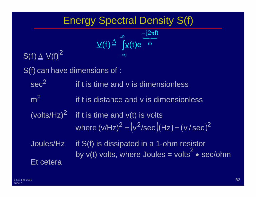
Energy Spectral Density S(f)

B2

)f(S 2∆

if t is time and v is dimensionlesssec2

if t is distance and v is dimensionlessm2

(volts/Hz)2 if t is time and v(t) is volts ( ) ( ) ( ) 222 sec/vHz/secv ==

if S(f) is dissipated in a 1-ohm resistor by v(t) volts, where Joules = volts2

• sec/ohm Joules/Hz

Et cetera

∫ ∞

∞−

π− ∆ ω=

j

e)t(v)f(V

6.661 Fall 2001

: of dimensions have can S(f)

(f) V

(v/Hz) where

� ft 2

Slide 8

Autocorrelation Function

B3

[ ] [ ])t(v)t(v)R( 2∗∞∫

)f(V)f(V)f(V)f(S 2=•= ∗

{ } ττ τ−∞ ∞−

∞ ∞−

∗∞ − ∫ ∫∫ d)t(v)t(vde)(R?)f(S jj

t′∆ tt ′− ′−

{ } { }v(t)e dt v (t )e dt∞ ∞ ′− π ∗ + π −∞ −∞

′ ′= •∫ ∫

constanttforof = ′

)f(S)(R ↔τClaim:

∫∫ ∫

∞ ∞−

∞

∞ +

==

=τ

)f(Sdt)t(v)0(R

dfe)f(S)(R 2

j

Therefore:

6.661 Fall 2001

.etc , J or sec v dtτ − ∆ τ ∞ −

.D.E.Q

τ − = τ ∞ −

τ π e dt f 2f 2

t d j2 ft j2 ft

t d ­sign Reverses

∞ −

∞ − τ π

Theorem s Parseval' df

f 2

Slide 9

Compact Transform Notation

B4

)f(S)f(V)(R

)f(V)t(v

2 ∆↔τ

↓↓ ↔ [ ] [ ]

[ ] [ ]22 Hz/vsecv

Hz/vv

↔

↓↓ ↔

[ ] [ ]Hz/JJoules ↔ If power is dissipated in a 1-ohm resistor

6.661 Fall 2001

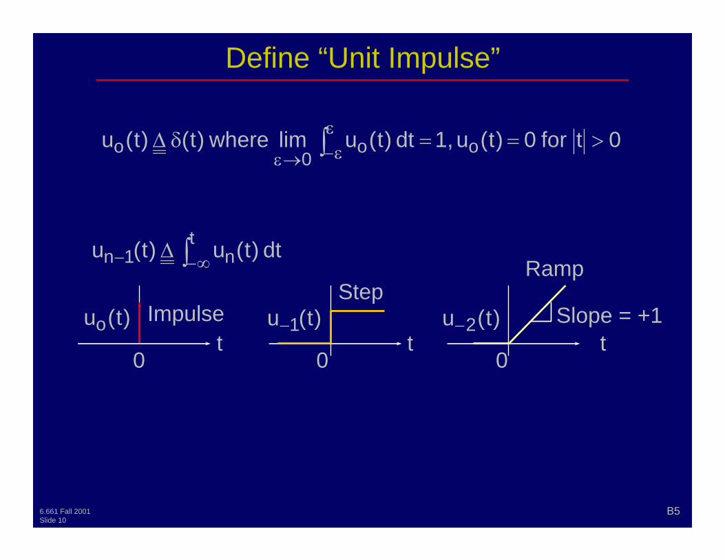
Define “Unit Impulse”

B5

0)t(dt)t(u)t()t(u oo0

o >==∫ ε

→ε

)t(uo Impulse

0 t

dt)t(u)t(u t n1n ∫− ∆

)t(u 1− )t(u 2−

Ramp

Slope = +1

0 0 tt

Step

6.661 Fall 2001 Slide 10

t for 0 u 1, lim where δ ∆ ε −

∞ −

Define “Convolution”

B6

)c(dt)b(t)t(a)t(b)t(a τ=∆∗ ∫ ∞ ∞−

0 t t τ

0 0

a(t) b(t) )(c)t(b)t(a τ=∗ *

6.661 Fall 2001 Slide 11

τ −

Useful Transformation Pairs for Pulses

C1

otj o e)f(A)tt(a ω−↔−

( ) fA)t(a ↔ dte)t(a)f(A j π∆ π−∞∫

1 o↔

1)t()t(uo ↔ energyHave ∞

( ) fAj)t(a ω↔′ dfe)f(A)t(a j π∞∫ =

( ) fe)t(a o tj o −↔ω

oo f2π≡ω

n n )j()t(u ω↔

( )j1/e)t(u t 1 ↔−

6.661 Fall 2001 Slide 12

f 2 ft 2 ∆ω ∞ −

(f) u

δ =

pulses) special as (treated

ft 2∞ −

f A

α + ω α −

Transforms: Even/Odd Functions

C2

e.g.

0 0 0 ttt

)t(a )t(ae )t(ao= +

( ){ }fAR)t(a ee ↔

( )[ ] ( )

( )[ ] ( )

(t)a(t)aa(t)

ODDta2/ta)t(a(t)a

EVENta2/ta)t(a)t(a

oe

oo

ee

+=

−=∆

−=−+∆where:

so:

{ })f(Amj)t(ao I↔

6.661 Fall 2001 Slide 13

− −

Transforms: Operators and Gaussians

C3

)f(A)f(A)t(a)t(a

)f(A)f(A)t(a)t(a

2121

2121

•↔∗

∗↔•

0 Aee

2 A)t(v 2/)(2/)/t( 22 σω−σ− ↔ πσ

∆

v(t)

σ

t

eAe2

A 22 )(22)2/(2

σω−↔πσ

↓

All Gaussians ↓

6.661 Fall 2001 Slide 14

σ τ −

Linear Systems

C4

∫ ∞ ∞ −

τ∆∗∆

=

d)t(h)(x)t(hx(t)y(t)

h(t)

Characterized by:

x(t)

h(t)f

=δ =

=

x(t) y(t)h(t)

CB)(AA ABBA

C)(AB)(AC)(BA

∗∗=∗∗

∗=∗

∗+∗=+∗ Note:

“Distributive” “Commutative” “Associative”

6.661 Fall 2001 Slide 15

← τ τ − integral" ion superposit "

where " Response, Impulse "

y(t) then (t), h(t) If

y(t) then (t), x(t) I: Test δ =

C) (B

Periodic Signals

E1

Tdt)t(v,dt)t(vAlthough T o

22 ∫∫ ∆∞= ∞

–T 3T2T0

v(t)

T

Infinite energy, finite power

Fourier Series:

2,...1,0,mwheredte)t(v T 1V 2/T

2/T t)T/2(jm

m ±±=∆ ∫ − π−

oo f2π=ω

( )1/TfeVv(t) o m

t m o ∆= ∑

∞

−∞=

π

1m = 0m =

6.661 Fall 2001 Slide 16

Period where ∞ < ∞ −

f 2 jm

Autocorrelation, Power Spectrum

E2

Autocorrelation Function:

( ) ∑∫ ∞

−∞=

τπ −

∗ =∆τ m

2 m

2/T 2/T

oeVdttv)t(v T 1)(R

Power Spectrum:

dte)(R T 1V 2/T

2/T 2

mm o∫ − τπ−τ=∆Φ

6.661 Fall 2001 Slide 17

τ − f 2 jm

f 2 jm

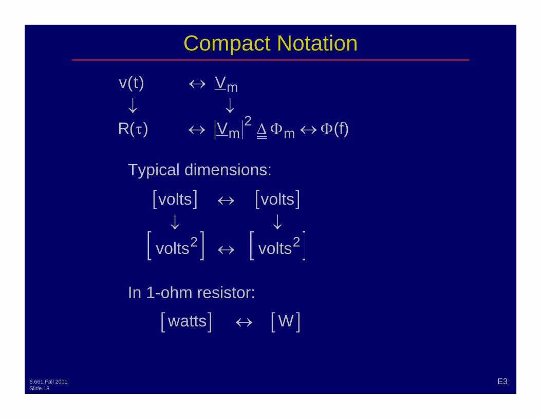
Compact Notation

E3

(f)V)(R

V)t(v

m 2

m

m

↔τ

↔

↓ ↓

[ ] [ ]W↔

In 1-ohm resistor:

Typical dimensions:

[ ] [ ]

[ ] [ ]22 voltsvolts

voltsvolts

↔

↓↓

↔

6.661 Fall 2001 Slide 18

Φ ↔ Φ ∆

watts

Transforms of Impulse Trains

E4

mVa/T)t(va

− 0 t fT/3− 0 T/2

0h/1− h/1

)(R τ

τ

ah

Area = τ

h/1

T/2

T/a2=

T/)0(R

h 1

T 2==

⎟ ⎠ ⎞

⎜ ⎝ ⎛ •

)t(v − 0 τ

)f(V 2 m

T/a2 )(R τ ( ) 2T/a

0 T/2 fT/3−

6.661 Fall 2001 Slide 19

T2 T2

.g.e

value impulse is a

value impulse becomes a area so h Let ∞ →

rea a

h a

h a 2 2

T2 T2

Φ →

Receiver Noise Processes

Receivers, Antennas, and Signals Professor David H. Staelin

6.661 Fall 2001 Slide 20

Random Signals

G1

and are unpredictable

Example: [ ]WH 1 z −

)f(Φ

MAXf0

Since we have infinite information for infinite time and a finite frequency band, then “V(f)” is not an analytic function and our approach must be different.

New definitions are required.

f

6.661 Fall 2001 Slide 21

Random signals generally have finite power, infinite energy,

Expected Value of x

G2

( )[ ] } ( )t i

ii ∫∑ ∞ →∆

oforFinite i

A “random signal” is drawn from some ensemble

( ) 1

x

i i

i

∆

ε

∑

t1 2t

t

t

)t(xi

)t(x j

( )[ ]ti

( ) ( ) ( )[ ]tv 2121v ∗∆φ

6.661 Fall 2001 Slide 22

( ) { dx x p x x p (t) x t x E ∞ −

(t) x ensemble infinite

x p

ensemble" "

x p

t v E t , t : Function ation Autocorrel

Stationarity

G3

transitions occur onlyat clock tickst

Otherwise v(t) is“Non-stationary”(time-origin sensitive)

1 1 0 0 1 0 1 2 3 4 5 6

( ) ( ) ( ) ∆−

τφ=∆+∆+φ

ttwhere t

2112

21v21v

v(t) is “wide-sense stationary” if:

( ) ( ) ( ){ }[ ] ( ) ( ) ( ){ }[ ]n21n21 ∆+∆+∆+=

v(t) is “strict-sense stationary” if:

( ) ( )T v TT

v(t) i1 v(t) v t

2T i

∗ −→∞

φ τ =

=

∫

v(t) is “Ergodic” if:

6.661 Fall 2001 Slide 23

– e.g.: 0 1 0

∆ τ φ =

, t , t all for t , t , t

g function any for t v ,..., t v , t v g E t v ,..., t v , t v g E

s wide-sense stationary and

lim dt,

.e., ensemble average time average

− τ

Transform Diagram: Random Signals

G4

v(t) ↔ (?)

↓ ↓

φv(τ) ↔ Φ(f)

[ V ] ↔ (?)

↓ ↓

[ V2 ] ↔ [ V2/Hz ]

Typical Sets of Units

[ V ] ↔ (?)

↓ ↓

[W] ↔ [W/Hz]

Power to 1-ohm resistor

Power spectral density

6.661 Fall 2001 Slide 24

Power Spectral Density

G5

Why use E[ ] if v(t) is ergodic?

⎥ ⎦

⎤ ⎢ ⎣

⎡ =Φ ∫ −

π− 2T

T j

T dte)t(v 1)f(

[ ] 2 T

2 T

2 T )f()f(E)f(where)f( Φ∆σ≠σ

Spectral resolution increases with T, becoming infinite as T → ∞ e.g.

Infinite information in finite bandwidth unless ensemble is averaged

t

Power Spectral Density Computation:

over successive intervals of width 2T. Use T adequate to

6.661 Fall 2001 Slide 25

∞ →

ft 2T2

E lim

!0 lim Because Φ −

For a single ergodic waveform, take ensemble average

yield desired or meaningful spectral resolution.