recasting human development measures - lse.ac.uk · sudhir anand working paper 23 ... i am...
TRANSCRIPT

Recasting Human Development
Measures
Sudhir Anand
Working paper 23
April 2018

III Working paper 23 Sudhir Anand
1
LSE International Inequalities Institute
The International Inequalities Institute (III) based at the London School of Economics and
Political Science (LSE) aims to be the world’s leading centre for interdisciplinary research on
inequalities and create real impact through policy solutions that tackle the issue. The Institute
provides a genuinely interdisciplinary forum unlike any other, bringing together expertise from
across the School and drawing on the thinking of experts from every continent across the
globe to produce high quality research and innovation in the field of inequalities.
For further information on the work of the Institute, please contact the Institute Manager, Liza
Ryan at [email protected].
International Inequalities Institute
The London School of Economics and Political Science
Houghton Street
London
WC2A 2AE
Email: [email protected]
Web site: www.lse.ac.uk/III
@LSEInequalities
LSE Inequalities
© Sudhir Anand. All rights reserved.
Short sections of text, not to exceed two paragraphs, may be quoted without explicit
permission provided that full credit, including notice, is given to the source.

III Working paper 23 Sudhir Anand
2
Abstract
The UNDP introduced three new human development measures in its 2010 Human
Development Report, which it has since continued to estimate and report on annually. These
measures are the geometrically-averaged Human Development Index (HDI), the Inequality-
adjusted Human Development Index (IHDI), and the Gender Inequality Index (GII). This paper
critically reviews these measures in terms of their purpose, concept, construction, properties,
and data requirements. It shows that all three measures suffer from serious defects, and
concludes that two of them are not fit for purpose. The paper suggests how HDI and GII might
be recast to overcome the problems identified and better reflect the purposes for which they
were devised.
Keywords: Human development; interpersonal inequality; zero values; gender
inequality; female disadvantage.
Editorial note and acknowledgements
I am extremely grateful to Selim Jahan and Amartya Sen for extended discussions and
insightful comments on the subject matter of this paper. I also wish to acknowledge the help I
received from members of the UNDP/HDRO team – including Milorad Kovacevic, Shivani
Nayyar and Heriberto Tapia. In addition, I would like to thank Zubin Siganporia and Devinder
Sivia who facilitated the computations and graphs in this paper.

III Working paper 23 Sudhir Anand
3
1. Introduction
In its 20th Anniversary Edition, the 2010 Human Development Report (HDR) introduced several
new measures of human development. The authors of the Report were rightly concerned
about rising inequalities and new vulnerabilities confronting many peoples and regions in the
world, which they argued required innovative public policies. In the Overview to the Report,
they declared that (UNDP 2010, p. 1):
“Addressing these issues requires new tools. In this Report we introduce three measures to
the HDR family of indices – the Inequality-adjusted Human Development Index, the Gender
Inequality Index and the Multidimensional Poverty Index. These state-of-the art measures
incorporate recent advances in theory and measurement and support the centrality of
inequality and poverty in the human development framework.”
These “state-of-the-art” measures are certainly new tools, yet arguably the most significant
‘measurement innovation’ of the 2010 HDR is that it presents “a refined version of the HDI,
with its same three dimensions” (UNDP 2010, p. 7) – but aggregates them using a geometric
mean. The original or old version of the HDI had aggregated the three dimensions using an
arithmetic mean.
Since the publication of these new measures, a large body of literature has arisen commenting
on their merits and their deficiencies. Some constructive criticism has also led to proposals for
different indices that appear to overcome particular shortcomings of the 2010 HDR measures.
In this paper I will not comment on the Multidimensional Poverty Index, but will critically review
the new ‘refined’ HDI, the Inequality-adjusted HDI (IHDI), and the Gender Inequality Index (GII)
– which are all still estimated and used in the post-2010 HDRs. The purposes and properties
of these three new indices – and the implications of their use – are not immediately apparent
from their construction. Hence I will attempt a detailed examination of these measures in
terms of their purpose, concept, construction, technical properties, and data requirements –
inter alia. There have also been some criticisms and misunderstandings of the pre-2010
human development measures, which I will likewise address in this paper. The investigation of
these measures is geared towards arriving at judgements about their future use in the HDR.
2. The old HDI and the new 2010 HDI
I start with the most significant and consequential change made in terms of measurement in
the 2010 HDR, namely that to the original HDI. In this section I compare the definition and
properties of the old HDI with those of the new 2010 HDI. The three core dimensions of the
HDI are life expectancy (LE), schooling (S) (in the old HDI measured through ‘literacy’ and

III Working paper 23 Sudhir Anand
4
‘school enrolment’, and in the new HDI through ‘mean years of schooling’ and ‘expected years
of schooling’), and per capita national income (Y).1
In the HDI, per capita income Y is entered in logarithmic form (ln Y) to reflect diminishing
returns to human development from additional income.
The three core dimensions are normalized to lie between 0 and 1 through the following
transformations:
𝐼𝐿𝐸 = 𝐿𝐸 − 𝐿𝐸𝑚𝑖𝑛
𝐿𝐸𝑚𝑎𝑥 − 𝐿𝐸𝑚𝑖𝑛
𝐼𝑆 = 𝑆 − 𝑆𝑚𝑖𝑛
𝑆𝑚𝑎𝑥 − 𝑆𝑚𝑖𝑛
𝐼𝑌 = ln (𝑌) − ln (𝑌𝑚𝑖𝑛)
ln (𝑌𝑚𝑎𝑥) − ln (𝑌𝑚𝑖𝑛)
where ‘min’ and ‘max’ denote the assumed (fixed) lower and upper bounds for each variable.
The aggregation formula used for these normalized indicators 𝐼𝐿𝐸 , 𝐼𝑆 , and 𝐼𝑌 was their
arithmetic mean prior to 2010. Let us call the old HDI, Hold.
Thus,
𝐻𝑜𝑙𝑑 = 1
3(𝐼𝐿𝐸 + 𝐼𝑆 + 𝐼𝑌)
Since HDR 2010, the aggregation formula for these indicators has been changed to their
geometric mean. Let us call the new 2010 HDI, Hnew.
Thus,
𝐻𝑛𝑒𝑤 = 𝐼𝐿𝐸1/3
× 𝐼𝑆1/3
× 𝐼𝑌1/3
How has this change affected the marginal contribution of each core dimension to the old and
new HDI, respectively?
1 In this section I adopt the notation used by Ravallion (2012) in his compelling criticism of the new HDI in terms of “troubling tradeoffs”, i.e. marginal rates of substitution between the core dimensions. But in this paper I do not discuss marginal rates of substitution between the core dimensions of HDI.

III Working paper 23 Sudhir Anand
5
This is shown by taking the first partial derivative with respect to that dimension. Here we are
primarily interested in the derivatives with respect to LE and Y.2 Through partial differentiation
with respect to LE and Y, respectively, we get:
𝜕𝐻𝑜𝑙𝑑
𝜕𝐿𝐸 =
1
3(
1
𝐿𝐸𝑚𝑎𝑥 − 𝐿𝐸𝑚𝑖𝑛) (2.1)
which is a constant, and
𝜕𝐻𝑜𝑙𝑑
𝜕𝑌 =
1
3(
1
ln (𝑌𝑚𝑎𝑥) − ln (𝑌𝑚𝑖𝑛)) (
1
𝑌) (2.2)
which is a decreasing function of Y, as required.
Note that the marginal contribution of LE to the old HDI is a constant (the upper and lower
bounds are fixed), and is therefore: (i) independent of the level of income Y and of schooling S;
and (ii) does not decline with the level of life expectancy LE (no diminishing returns to life
expectancy).
Now let us calculate the marginal contributions of LE and Y for the new HDI. After partial
differentiation and some manipulation, we find that:
𝜕𝐻𝑛𝑒𝑤
𝜕𝐿𝐸 =
1
3(
1
𝐿𝐸𝑚𝑎𝑥 − 𝐿𝐸𝑚𝑖𝑛) (
𝐼𝑆1/3
. 𝐼𝑌1/3
(𝐿𝐸 − 𝐿𝐸𝑚𝑖𝑛)2/3) (2.3)
and
𝜕𝐻𝑛𝑒𝑤
𝜕𝑌 =
1
3(
1
ln (𝑌𝑚𝑎𝑥) − ln (𝑌𝑚𝑖𝑛)) (
𝐼𝑆1/3
. 𝐼𝐿𝐸1/3
𝑌. (ln (𝑌) − ln (𝑌𝑚𝑖𝑛))2/3) (2.4)
From equation (2.3), it follows that for the new HDI the contribution of an extra year of life
expectancy LE depends positively on the level of income Y (𝐼𝑌) and of schooling S (𝐼𝑠), and
negatively on the level of LE. But do we really want a human development index to satisfy
these properties? I attempt to address this question below.
From equation (2.4), it follows that for the new HDI an extra unit of per capita income Y makes
a larger contribution to 𝐻𝑛𝑒𝑤 the larger is LE (𝐼𝐿𝐸) and the larger is S (𝐼𝑆).
2 The partial derivatives with respect to S are given by simply replacing LE with S in equation (2.1), and by switching LE and S in equation (2.3) in the text.

III Working paper 23 Sudhir Anand
6
In other words, the cross-partial derivatives with respect to LE and Y are positive:
𝜕2𝐻𝑛𝑒𝑤
𝜕𝑌 𝜕𝐿𝐸 =
𝜕2𝐻𝑛𝑒𝑤
𝜕𝐿𝐸 𝜕𝑌 > 0 (2.5)
But do we really want these cross-partial derivatives to be positive, and if so why? Why should
an extra year of life contribute more to the HDI at a higher level of income, or of schooling, and
less at a lower level of income and schooling?
A critically important feature of the old HDI is that the contribution of each variable is
independent of – and separable from – the levels of the other variables. Hence the original
HDI attaches the same value to an extra year of life (male or female) in any country and at any
income or schooling or life expectancy level. This is justifiable under a straightforward ethic of
‘universality of life claims’ (see Anand and Sen 1996, pp. 1-3; Anand and Sen 2000b, pp.
2029-30). It would go against the tenets of human development to intrinsically value an extra
year of life less in poorer countries than in richer countries, and less in countries with a lower
than a higher level of education – but that is exactly what the new HDI does.
The original HDI is thus quite different in this important respect from the new HDI, and from
other indices proposed in UNDP (2010) and Alkire and Foster (2010), whose valuation of an
extra year of life depends positively on the level of income and of education, and negatively on
the level of life expectancy.3
These and several other serious problems with using the geometric mean for aggregation are
demonstrated in the next sections of this paper. In the concluding section, a recommendation
is made to revert to the arithmetic mean in aggregating the normalized indicators 𝐼𝐿𝐸, 𝐼𝑆, and
𝐼𝑌.
2.1. Justifications provided for aggregation using a geometric mean
An early commentator who expressed a preference for aggregating the three HDI indicators
(normalized dimensions) by use of a geometric mean was Desai (1991), who has otherwise
made some helpful contributions to the human development agenda. In relation to the original
HDI, he argued that (Ibid., p. 356):
3 Chakravarty’s (2003) generalized human development index avoids having positive cross-partial derivatives between different dimensions, and has other desirable properties (including additive separability). Yet it is formulated to display diminishing returns to life expectancy. Chakravarty (2011b, p. 520) argues that: “Since each of the three attributes of income, health, and education is a ‘good’, the law of ‘diminishing marginal utility’ should apply to each of them. In other words, we can measure all the three indicators by using any increasing and strictly concave transformation.”

III Working paper 23 Sudhir Anand
7
“Other improvements which need to be pursued are to examine the robustness of the ranking
to other weighting schemes. Thus additivity over the three variables implies perfect
substitution which can hardly be appropriate. Going back to the notion of capabilities as being
corealisable, one should try to restrict the substitutability as between the basic variables. One
way to do this would be to use a log additive form. This would make the deprivations
multiplicative, each feeding off the other. Such a weighting would heighten the plight of the
very poor and make the gradient of human development steep.”4
But why does “corealisability” imply that we “should try to restrict the substitutability as
between the basic variables”? Moreover, do we really want each [variable] to “feed off” the
other? Presently, I will comment on precisely why we do not want that. Also, it is not clear
what is meant by making “the gradient of human development steep”. With respect to what is
the gradient of human development being made steep?
The Human Development Report 2010 itself suggested the following justification for using the
geometric mean. The key summary Box 1.2 in UNDP (2010, p. 15) states:
“We also reconsidered how to aggregate the three dimensions. A key change was to shift to a
geometric mean (which measures the typical value of a set of numbers): thus in 2010 the HDI
is the geometric mean of the three dimension indices. Poor performance in any dimension is
now directly reflected in the HDI, and there is no longer perfect substitutability across
dimensions. This method captures how well rounded a country’s performance is across the
three dimensions. As a basis for comparisons of achievement, this method is also more
respectful of the intrinsic differences in the dimensions than a simple average is. It recognizes
that health, education and income are all important, but also that it is hard to compare these
different dimensions of well-being and that we should not let changes in any of them go
unnoticed.”
The arguments in this UNDP (2010, p. 15, Box 1.2) paragraph above are somewhat unclear
and difficult to understand. Why does the geometric mean measure “the typical value of a set
of numbers”? One might have thought that the “typical value” is the mode of a distribution, not
its geometric mean. “Poor performance in any dimension” was always “directly reflected” in
the old HDI – it is not the case that the new HDI has only now begun to reflect it through
geometric averaging. Next, it is not clear how “this [geometric averaging] method is also more
respectful of the intrinsic differences in the dimensions than a simple average is”.5
4 Sagar and Najam (1998, p. 252) use similar arguments to recommend a multiplicative aggregation scheme (without taking the cube root to form the geometric mean); thus they state that “…a better strategy to estimate national HDIs would be through a product of the three component indices.” 5 Ravallion (2012, pp. 202-3) has commented similarly on some of the statements in UNDP (2010, p. 15, Box 1.2).

III Working paper 23 Sudhir Anand
8
UNDP (2010, p. 15, Box 1.2) ends by stating that “we should not let changes in any of [the
different dimensions of well-being] go unnoticed.” However, it is precisely the use of the
geometric rather than the arithmetic mean which can allow “changes in any of them” to go
unnoticed. Consider the following simple example aggregating the three dimensions by use of
the geometric and arithmetic mean, respectively. Suppose (ILE, IS, IY) = (0.5, 0.4, 0.0), then
Hnew = 0.0 and Hold = 0.3. Now raise ILE from 0.5 to 0.8 while keeping the other two indicators
the same as before. Then Hnew = 0.0 still, but Hold = 0.4. Unlike what UNDP (2010, p. 15, Box
1.2) claims, using the geometric mean of the three indicators does let changes in an indicator
go unnoticed! In contrast, the old HDI does not “let changes in any of them go unnoticed”. In
the above example, Hold rises from 0.3 to 0.4 as a result of the change in ILE from 0.5 to 0.8,
but Hnew remains the same at 0.0.
In equation (2.3) for ∂Hnew/∂LE above, it is clear that Hnew attaches a low value to extra life in
poorer compared to richer countries. The marginal contribution of an extra year of longevity
depends directly on 𝐼𝑌1/3
(and on 𝐼𝑆1/3
). So the closer is IY (or IS) to zero, the lower the value put
on an extra year of life in Hnew. Take the case of Zimbabwe in 2010 where its per capita
national income is PPP$176 – very little above the Ymin of PPP$163. The estimation of IY by
Chakravarty (2011b, p. 521) shows that it is indeed very low (= 0.01). Given this fact, he
calculates that an increase in life expectancy in Zimbabwe by 50 years will not enable its Hnew
to increase by even 0.1.
Ravallion (2012) poses a related question about Zimbabwe’s 2010 HDI, which has the lowest
value at 0.14 of any country – with the next lowest HDI value being that of the Democratic
Republic of Congo (DRC) at 0.24. Ravallion (2012, p. 204) asks: “What then would it take to
get Zimbabwe off the bottom rung of the HDI ladder? To answer this one cannot simply
extrapolate linearly using the marginal weights (i.e. first partial derivatives), but one must solve
the appropriate nonlinear equation for the HDI (equating Zimbabwe’s HDI to that of the DRC,
while holding schooling and income constant at Zimbabwe’s current level, then solving for the
required value of LE). On doing so one finds that Zimbabwe would need a life expectancy of
154 years! And that would only get Zimbabwe to the DRC’s HDI. That does not sound like a
promising route for getting off the bottom rung of the HDI ladder.”
This unacceptable situation arises because of the direct dependence of the rate of change of
Hnew with respect to LE on other variables, viz. Y and S. It results precisely because of the so-
called multiplicative “feeding off” each other recommended by some supporters of Hnew. The
old HDI, Hold, is immune from such problems because it values the contribution of longevity at
a constant rate that is independent of the level of the other variables (see equation (2.1)
above).

III Working paper 23 Sudhir Anand
9
2.2. Disaggregating the Human Development Index
The old HDI, Hold, is additively separable in its component indicators; hence the contribution of
each component can be separately identified and quantified as a percentage of the overall
index. By contrast, it is not possible to disaggregate or ‘decompose’ the value of the new HDI,
Hnew, into separable contributions of its three components.
Additive separability of the HDI is clearly a desirable property if we want to measure the
individual contribution of each of its core dimensions – life expectancy, schooling, and
income.6 It allows us to isolate the factors (and policies) that lead to the HDI value of one
country being different from that of another, and likewise to changes in the HDI value of a
given country over time.
Unlike an arithmetic mean, it is not possible to disaggregate a geometric mean into additively
separable components. The new HDI, being a geometric mean, is multiplicatively – but not
additively – separable. This implies that its logarithm will be additively separable. But
decomposing the logarithm of the new HDI into the logarithms of its component indicators is
quite different from decomposing the new HDI itself. Taking logarithms cannot offer a viable
route to identifying the contribution of each component of the index proper.
Unfortunately, however, this is exactly what Permanyer (2013, p. 16) does in a different
context with respect to an index that he proposes: the Women Disadvantage (or WD) index.
WD is constructed as a geometric average of its components (similarly to the new HDI) and is
discussed in Section 6 of this paper. Permanyer calls the additive separability property
‘decomposition’,7 and claims to ‘decompose’ (additively disaggregate) the index WD, stating
that WD has the “advantage of being decomposable by subcomponents, thus allowing the
calculation of the percentage contribution of each individual subcomponent to the aggregate
value of the index” (Ibid., p. 16). This is incorrect because it is not possible to decompose
(additively disaggregate) the index WD itself, but only the logarithm of WD (Ibid., p. 26,
endnote 12).8
6 Thus in the case of Hold, the respective contributions of LE, S, and Y are (1/3)ILE/Hold, (1/3)IS/Hold, and (1/3)IY/Hold – which add up to 1 (or 100 percent). 7 Such ‘decomposition’ is not to be confused with decomposing an inequality index between- and within- population subgroups. The old HDI is additively separable (‘decomposable’) across its component indicators (ILE, IS, IY), but not across population subgroups; this is because the income indicator IY is non-linear in Y (IY is linear in ln(Y), not in Y). 8 In a different context where I discuss inequality decomposition (Anand 1983, pp. 89-92), I show that a monotonic increasing transform of the Atkinson inequality index is decomposable between- and within- population subgroups, but the Atkinson index itself is not. I conclude there that the Atkinson index cannot be used to decompose inequality.
III Working paper 23 Sudhir Anand
10
Permanyer (2013, pp. 20-21, Figure 7) must therefore be measuring the percentage
contribution of the logarithm of each subcomponent to the logarithm of WD and not, as he
states, “the values of WD and the percentage contribution of its subcomponents to the
aggregate values of WD” (Ibid., p. 20). Permanyer (2013, p. 24) incorrectly concludes that
“WD has the further advantage of being decomposable into its components, thus facilitating
the understanding of the internal structure of the index and allowing us to easily compute the
percent contribution of each individual subcomponent to the aggregate value of the index.”
2.3. The bounds for normalizing ILE, IS, and IY in the HDI
The 2010 HDR modified the old HDI bounds that were used to normalize the three core
dimensions to a common scale. Previously it was assumed that life expectancy was bounded
below (min) by 25 years and above (max) by 85 years. In the 2010 HDR these bounds were
changed to 20 years (min) and 83.2 years (max) (Japan’s life expectancy). The bounds for
other variables were also changed in HDR 2010.
The new HDI (Hnew), based on the geometric mean of the component indicators, is extremely
sensitive to the lower bound chosen – as illustrated in this paper when the value of a core
dimension approaches its lower bound, i.e. the corresponding normalized indicator approaches
zero. Unlike for Hnew, the lower bound is not critical if an arithmetic mean is used for averaging
these indicators – as in the old HDI.
The question of bounds needs to be re-examined in-house at UNDP if it decides to revert to
arithmetic averaging of the normalized indicators of HDI. In this case, a range for life
expectancy of 50 years would seem reasonable, with the min set at 40 years and the max at
90 years. For per capita national income the min bound could be maintained at PPP$163
(Zimbabwe in 2008) – as in HDR 2010. This will clearly demonstrate the contrast made
through averaging the indicators using the arithmetic and geometric mean, respectively. The
upper bound is open for discussion (and experimentation), and could be capped at the 2010
max value of PPP$108,211 (United Arab Emirates in 1980).
The new education variables should continue to have lower bounds (min) of zero. The upper
bounds (max) for mean years of schooling (MS) and for expected years of schooling (ES) are
open for discussion, but should perhaps be set at higher than their 2010 values of 13.2 years
(US in 2000) and 20.6 years (Australia in 2002), respectively. With arithmetic averaging
reinstated in the HDI, its schooling indicator IS should be formed through taking the arithmetic
mean of its subcomponent (MS and ES) indicators – not their geometric mean as in the 2010
HDI.

III Working paper 23 Sudhir Anand
11
3. The Inequality-adjusted HDI (IHDI)
The human development index – old and new – is an aggregate measure estimated at the
level of a country or a population group, such as a gender group or province within a country.
The core dimensions of the HDI are country- or group-level variables: life expectancy at birth,
mean and expected years of schooling, and the logarithm of gross national income per capita.
It is tempting to consider disaggregating these variables to the level of individual person –
rather than to use them only at country- or group-level. This disaggregation, if it were possible,
would enable the measurement of interpersonal inequality within each dimension, and for all
three dimensions together if their joint distribution was known. With such information we would
have the means to make an adjustment for interpersonal inequality in the aggregate HDI.
Foster et al. (2005) initiated this type of study, which was later refined and developed by Alkire
and Foster (2010)9 – two authors who have elsewhere made some valuable contributions to
measuring poverty and inequality. To estimate an inequality-adjusted human development
index (IHDI), the 2010 HDR embraced in full the Alkire and Foster (2010) methodology and
associated recommendations (see UNDP 2010, pp. 217-19, Technical Note 2).
The 2010 HDR motivated the IHDI as follows:
“The IHDI takes into account not only a country’s average human development, as measured
by health, education and income indicators, but also how it is distributed. We can think of each
individual in a society as having a ‘personal HDI.’ If everyone had the same life expectancy,
schooling and income, and hence the average societal level of each variable, the HDI for this
society would be the same as each personal HDI level and hence the HDI of the ‘average
person.’ In practice, of course, there are differences across people, and the average HDI
differs from personal HDI levels. The IHDI accounts for inequalities in life expectancy,
schooling and income, by ‘discounting’ each dimension’s average value according to its level
of inequality. The IHDI will be equal to the HDI when there is no inequality across people, but
falls further below the HDI as inequality rises. In this sense, the HDI can be viewed as an
index of ‘potential’ human development (or the maximum IHDI that could be achieved if there
were no inequality), while the IHDI is the actual level of human development (accounting for
inequality). The difference between the HDI and the IHDI measures the ‘loss’ in potential
human development due to inequality” (UNDP 2010, p. 87).
9 This paper by Alkire and Foster was published as UNDP Human Development Reports Research Paper 2010/28 in October 2010 – see References. Sabina Alkire and James E. Foster also published a paper with the same title and content as an OPHI Working Paper in July 2010: “Designing the Inequality-Adjusted Human Development Index (HDI)”, OPHI Working Paper No. 37, Oxford Poverty & Human Development Initiative (OPHI), Queen Elizabeth House, Oxford, July. https://ora.ox.ac.uk:443/objects/uuid:f0299b95-2c81-4f29-8d86-71396d6b6dfd. Page references to their paper in this document are to the October 2010 Human Development Reports Research Paper, not the OPHI paper.

III Working paper 23 Sudhir Anand
12
Alkire and Foster (2010, p. 2) set out the framework for determining IHDI in the following
terms: “[T]he distribution of the three dimensions of human development in a population can be
represented by a matrix X whose rows give the achievements of a person across the
dimensions of income, education and health, and whose columns give the distributions of an
achievement across the population.”
The matrix X = (xij) has n rows (one for each person) and 3 columns (one for each dimension
of human development), with xij denoting person i’s ‘level of human development’ in dimension
j. Alkire and Foster then calculate the ‘equally distributed equivalent achievement’ Xede as a
“(1 – ε)-average” of the 3n elements of the nx3 matrix X. When ε = 1, Xede is the geometric
mean calculated across the 3n elements – which thus accounts for inequality both within and
across dimensions. The authors label this geometric mean H1, and it is easy to see that it
satisfies their desired properties of path independence and subgroup consistency. Since each
multiplicative term in the geometric mean H1 is (xij)1/3n, the 3n elements (xij) of the matrix X can
be multiplied in any order – row first column second, or column first row second, or in any
zigzag path – to arrive at their ‘path independent’ measure H1. Alkire and Foster (2010, p. 7)
propose the index H1 as the inequality-adjusted HDI (IHDI) – which they state “has particularly
useful interpretations and properties”.
Let us examine a key property of H1. As a geometric mean across dimensions and people, H1
has positive cross-partial derivatives with respect to xij and xi´j´ where i´≠ i or j´≠ j, for i´, i = 1,
2,…, n and j´, j = 1, 2, 3. In other words, the cross-partial derivative is positive with respect to
different dimensions j and j´ for the same person i, or for the same dimension j for different
persons i and i´, or for different persons i and i´ and different dimensions j and j´. In the case
of the same person (i), the cross-partial derivative being positive for different dimensions (j and
j´) in H1 is the individual-specific counterpart of the corresponding cross-partial derivatives of
Hnew discussed in Section 2. For example, in H1 an extra year of schooling (j´) for person (i),
xij´, will contribute less to H1 the lower is his or her own income (j), xij. It is not obvious that this
is a desirable property of a human development index, even adjusted for inequality. As
another example, an extra year of schooling (j´) for a poor individual (i), xij´, will contribute less
to H1 the lower is the income (j) of some very rich individual (i´) in the population, xi´j. It would
seem difficult to justify such intrinsic valuations in an index of human development.10
10 I have deliberately side-stepped the question of whether Alkire and Foster’s income entry for each person i in the matrix X should be the logarithm of his or her income or simply their unlogged income. Adjustment for inter-individual inequality in the aggregate HDI, whose income component is the logarithm of gross national income per capita, ln Y, would seem to require that its individual-specific counterpart is the logarithm of person i’s income – so that equality within each dimension results in the aggregate HDI. Furthermore, I am assuming that the elements of the matrix X are the individual-specific normalized indicators (corresponding to the aggregate measures ILE, IS and IY) rather than the core variables themselves; this is how I read Alkire and Foster (2010, p. 2, Section 2.1). But neither of these issues affects my conclusions in the above paragraph about the positive sign of the relevant cross-partial derivatives of H1.
III Working paper 23 Sudhir Anand
13
Apart from H1, Alkire and Foster (2010, p. 8) also propose an alternative HDI that suppresses
within-dimension (across people) inequality, and call this measure H1*, stating that “one can
define a base human development index H1* that retains the cross-dimensional inequality but
suppresses within-dimension inequalities.”11 Their base human development index H1* is, of
course, exactly the new HDI of UNDP (2010), which I have called Hnew in this paper. Alkire
and Foster go on to state that: “Like the [old] HDI, the index H1* ignores within dimension
inequalities; unlike the [old] HDI, it takes into account inequality across dimensions” (Ibid., p.
8).
Because H1* uses two different means – arithmetic and geometric – in its aggregation, rather
than the geometric mean across all elements of the matrix X as H1 does, H1* does not possess
the “desirable property of path independence” (Alkire and Foster 2010, p. 9). The authors
state that by first averaging arithmetically within dimensions, and then applying the geometric
mean across dimensions, is not the same as “first applying the geometric mean to assess an
individual’s development level and then applying the arithmetic mean across the individual
levels” (Ibid., p. 9). They conclude that: “This implies that there are two possible ways of
evaluating potential human development, and one way must be chosen. As we note below,
the absence of individual data with which to compute the latter option leads us to the former
option and H1*” (Ibid., p. 9).
Having thus opted for H1*, i.e. for Hnew, Alkire and Foster (2010) go on to provide an example
of its estimation – and that of H1 – for Norway and Haiti (Ibid., pp. 26-28). Their estimation of
H1 requires information on three within-dimension geometric means (or values of the Atkinson
inequality index for ε = 1). But no sources for the latter numbers are provided in their paper, so
it is possible that their example is based on assumed rather than real data.12
There is, in any case, a prior conceptual problem in trying to estimate H1, i.e. IHDI. It requires
information at the individual level for each dimension of HDI – viz. the (xij) in the matrix X,
where xij is person i’s ‘level of human development’ in dimension j. However, it is difficult to
imagine how an “individual’s development level” (Alkire and Foster 2010, p. 9) or a “personal
HDI level” (UNDP 2010, p. 87) or “the distribution of human development across people”
(Foster et al. 2005, p. 6) might be determined for the dimension of life expectancy at birth and
the sub-dimension of expected years of schooling. Unlike income and actual years of
schooling which an individual person possesses, life expectancy at birth and expected years of
schooling are not individual-specific possessions. Indeed, they can only be defined at group
11 In the nx3 matrix X, this is represented by replacing every element in a column of the matrix X by the arithmetic mean of that column. 12 In their example, income seems to have been entered in unlogged form, and GNI per capita for Norway at “PPP US$ 58,810” exceeds the upper income cutoff of “51,200 $”.

III Working paper 23 Sudhir Anand
14
level – e.g. life expectancy at birth in a country or a gender group or a province.13 The notion
of an ‘individual life expectancy at birth’ which is different for different persons in the same
group is not coherent. By definition, every individual in any particular group with respect to
which life expectancy at birth is calculated must have the same life expectancy at birth. Hence
the concept of individual “inequalities in life expectancy” (or individual inequalities in expected
years of schooling) seems to be misconceived. 14 This is unlike the case for the other
components of HDI, viz. total national income or total years of schooling in a country, for which
an individual-specific counterpart is well defined.
Hence, two of the variables in HDI which are defined only at aggregate level – life expectancy
at birth and expected years of schooling – do not have counterparts at the individual level. So
IHDI cannot measure inter-individual inequality in the variables of HDI.
If, however, different variables were to be used to measure interpersonal inequality in health or
in schooling, we would not be calculating an inequality-adjusted HDI. An adjustment for
inequality applied to some variable that is not a component of HDI cannot generate an
inequality-adjusted HDI. It would not amount to “…‘discounting’ each dimension’s average
value according to its level of inequality” (UNDP 2010, p. 87, italics added). A composite index
formed by an adjustment for inequality in a non-HDI variable is clearly not consistent with the
“general mean of general means” approach to constructing IHDI in Alkire and Foster (2010).
Despite its many theoretical properties such as path independence and subgroup consistency,
IHDI is compromised as an index by its failure to be consistent in both concept and
measurement at the aggregate and individual levels. It also has other shortcomings,15 some of
which are noted by Bossert et al. (2013). Importantly, IHDI suffers from the zero-value
problem of geometric means, which I discuss separately in Section 4. The additional and
13 Alkire and Foster (2010, p. 26) do recognize that: “Life expectancy data are commonly used in aggregate indicators but are not available at the individual level, nor by population subgroups in all countries.” However, it is not the availability of life expectancy data at the individual level that is the problem, but the very concept itself. 14 UNDP (2010, pp. 217-18) and Alkire and Foster (2010, p. 26) do have very brief discussions of their estimation of interpersonal inequality in life expectancy, but it is not clear exactly what they do, what it means, or how it relates to the concept in question. For example, Alkire and Foster (2010, p. 26) state that: “It is possible to estimate a lower bound of inequality by constructing the arithmetic and general means of the distribution of life expectancy for different age cohorts of the population, relying on data from life tables.” However, it is not evident how life expectancy for different age cohorts of the population informs the interpersonal distribution of life expectancy at birth, which is the longevity concept in the aggregate HDI. 15 UNDP (2010, p. 219) laments a current shortcoming of IHDI: “The main disadvantage of the IHDI is that it is not association sensitive, so it does not capture overlapping inequalities.” This comes about because IHDI is estimated without data for each individual “from a single survey source”. With data on each individual (even if from multiple sources), it would be possible to construct the nx3 matrix X whose row vectors represent the 3 ‘human development’ achievements (‘personal HDI’) for the same individual, including his or her deprivation in all 3 dimensions. So in principle “overlapping inequalities” will be captured in IHDI by the geometric mean being taken across each row (i.e. across dimensions) – and then across each column (i.e. across persons) – of the nx3 matrix X. However, as argued in the text, the concept of a ‘personal HDI’ is not well-founded, and a consistent matrix X based on it is unlikely to materialize in practice.
III Working paper 23 Sudhir Anand
15
multidimension inequality considerations incorporated into IHDI would seem to overburden the
already problem-ridden new HDI, viz. H1* or Hnew.
In this context, it would be hard to disagree with the general sentiment expressed by Amartya
Sen who has noted that: “It would be a great mistake to cram more and more considerations
into one number like the HDI, … the human development approach is sophisticated enough to
accommodate new concerns … without muddled attempts at injecting more and more into one
aggregate measure” (UNDP 2010, p. vii).
4. Treatment of zero values in the HDR 2010 indices
There are three new indices in HDR 2010 that are based on, and constructed using, the same
underlying method of aggregation – the geometric mean. These are the new Human
Development Index (Hnew), the Inequality-adjusted Human Development Index (IHDI), and the
Gender Inequality Index (GII). In this section I investigate how the proponents of these new
indices have addressed the issue of zero values in the data.
UNDP (2010, p. 218) attempts to avoid the issue by claiming that the geometric mean “does
not allow zero values”.16 It is not clear whence this arises because the definition of geometric
mean provided by UNDP itself (2010, p. 218, equation (1), and also column 2) certainly
“allows” the geometric mean to be calculated for any set of non-negative numbers, which
obviously includes zero.
The definition of the geometric mean of three (or n) non-negative numbers is the cube (or nth)
root of the product of the numbers.17 If one of the numbers should happen to be zero, the
product of the numbers will be zero and hence so will its cube (or nth) root – i.e. the geometric
mean will be zero. Indeed, this is sometimes regarded as a virtue of the geometric mean
because it gives the smallest number in the set the largest weight.
To see this, note that the number x enters the formula for the geometric mean of three non-
negative numbers (x, y, z) as x⅓. The partial derivative of x⅓ with respect to x is (⅓)x−⅔, which
tends to ∞ as x tends to 0. So x⅓ approaches 0 rapidly as x approaches 0. This property is
important in understanding the consequences of replacing a number like x that is zero with an
16 If this were actually true, which it is not, and valid zero values were observed in the data, then the geometric mean should simply not be used – because it “does not allow zero values”. 17 The definitive work on different types of means, and the inequalities associated with them, is the classic treatise
by the 20th century mathematicians Hardy, Littlewood and Pólya (1952). They define the geometric mean G of any set of n non-negative numbers as the nth root of their product (Ibid., p. 12, equation (2.1.7)), and both “allow”
and discuss situations when G = 0 as a result of one or more of the n non-negative numbers being zero (Ibid., pp. 13-15, 21, 26, etc.).

III Working paper 23 Sudhir Anand
16
artificial small positive number in the desire to generate a non-zero geometric mean. The
geometric mean will be highly sensitive to the particular small positive number chosen as
replacement for the zero value: the mean can be made as close – and as rapidly – as one likes
to zero by choosing a small enough positive number.
In calculating IHDI, UNDP (2010, p. 218) makes the following arbitrary replacements for what it
considers “extreme values” – which are actually observed and valid numbers in the data. In
particular, it deals with 0 years of schooling and zero incomes together with “extremely high
incomes” as follows:
“For mean years of schooling one year is added to all valid observations to compute the
inequality. Income per capita outliers – extremely high incomes as well as negative and zero
incomes – were dealt with by truncating the top 0.5 percentile of the distribution to reduce the
influence of extremely high incomes and by replacing the negative and zero incomes with the
minimum value of the bottom 0.5 percentile of the distribution of positive incomes.”
In calculating GII, discussed later in Section 8, UNDP (2010, p. 220) makes the following
replacements to zero values for female parliamentary representation: “The female
parliamentary representation of countries reporting 0 percent is coded as 0.1 percent because
the geometric mean cannot have zero values and because these countries do have some kind
of political influence by women”. One might well ask why 0.1 percent and not 0.01 percent or
0.001 percent, or any other artificial small number. Another curious argument here is the
defense provided that “these countries do have some kind of political influence by women”.
But if political influence by women other than through parliamentary representation is to be
included, then this needs to be explicitly defined and measured for all countries – and not
inserted in an arbitrary manner just for countries with zero female parliamentary
representation. If a different variable is envisaged (e.g. ‘parliamentary representation’ plus
‘non-parliamentary political influence’), it must be identified and quantified for every country in
order that consistent international comparisons are made.
In their treatment of zero values in Hnew and IHDI, Alkire and Foster (2010, pp. 31-32) remind
us that:
“The geometric mean is highly sensitive to the lowest values in the distribution, and particularly
to the lower bound. When data are well defined, this is a signal strength of the measure: it
emphasizes the situation of the poorest poor. However in situations where data do not have a
natural zero, or where the lowest values are not well defined, the sensitivity of the final
measure to these values is problematic. The IHDI in its current form is not immune from
problems. Income data have zero and negative values, which must be replaced by some low
value [sic], and the final inequality measure will be sensitive to those replacement values. A
III Working paper 23 Sudhir Anand
17
similar situation exists for years of schooling, in which many zero values are present. The
current IHDI has made some specific replacements; however, sensitivity analysis reveals that
the rankings are indeed changed by different replacements. Hence while the zero value
replacement should be informed by the sensitivity tests, it may best be chosen by normative
logic in order to create a ratio scale variable.
For example, in income space, the present procedure replaces the zero and negative values
by some fixed amount such as the income of the person at the 2.5 percentile of the population,
whatever that may be. Alternatively, the replacement could be by a fixed value that is
translated into the comparable PPP value for each country, or by a fixed nominal value.
Careful consideration of this issue and of parallel issues in education is warranted.”
The question still arises as to why income data that have zero (or negative) values must “be
replaced by some low value”, and similarly why zero years of schooling must be replaced by
some positive value.18 Note that the validity of the empirically observed data is not being
questioned by the authors. If for these valid zero-value data the index becomes degenerate
(zero) – or incalculable – then it is the index that is invalid or inappropriate for the task at hand,
not the data. Therefore, it is the index that should be discarded and replaced, not the valid
zero-value data.19
Some decades ago, I faced a similar situation in my work on Malaysian income distribution
(Anand 1983). There were perfectly valid zero-income individuals in the Post Enumeration
Survey data that I was analyzing in order to measure and decompose income inequality in the
country. Given this fact, I simply could not use certain inequality measures and commented as
follows (Anand 1983, p. 84): “Unfortunately, the Atkinson index cannot be computed on the
Malaysian data for values of ε > 1 because of the presence of zero-income individuals … the
equally distributed equivalent income yede is not defined in this case.”20
Unlike the proponents of the new human development measures who choose to substitute an
inconvenient zero value with a small positive number, I did not replace zero incomes with a
‘small positive income’. Rather, I argued that: “This is not simply a technical problem which
18 Amartya Sen has drawn my attention to the “horrendous discontinuity” that results in the index (geometric mean) when a valid zero observation for one of its variables, x, is replaced by some positive value such as 1. Let
the geometric mean G of three non-negative numbers (x, y, z) be x⅓×y⅓×z⅓, and consider G as a function of x
holding y, z > 0 constant. Then as x → 0, G → 0. But at x = 0 there is a sharp discontinuity because the index G
suddenly jumps up to a positive number with the replacement (viz. to G = 1⅓×y⅓×z⅓)! 19 In Section 6, I comment on Klasen and Schüler’s (2011) response to observing zero values in the data. As I understand it, they seem content with a calculation that results in a zero geometric mean – as long as it is “borne in mind when interpreting the figures” (Ibid., p. 22). 20 I also noted that: “For the case of ε = 1, yede is simply the geometric mean income of the distribution, and the Atkinson index is 1 minus the ratio of the geometric to the arithmetic mean income. With a single zero-income individual, the geometric mean is zero and the Atkinson index takes the value unity” (Anand 1983, p. 84, footnote 25).

III Working paper 23 Sudhir Anand
18
can be got around by assigning a small positive income to zero-income individuals, as is
sometimes suggested. The value of the inequality index will depend crucially on the particular
income assigned, and it can be made arbitrarily close to unity (perfect inequality) by choosing
a small enough level” (Ibid., p. 84).
For the same reason, in a distribution with zero incomes, I could not use two other inequality
indices that are sometimes used for decomposition – viz. Theil L and the variance of log-
income. I argued (Ibid., p. 308) that: “The measures are not defined if there is a person in the
distribution with zero income. Unfortunately, this happens to be the case with some of the
Malaysian distributions considered. To overcome this problem, some have suggested that the
zero-income recipients be assigned a small positive income (such as 1). But the choice of the
amount assigned makes all the difference to the value of the measure. The sensitivity of the
measure to this arbitrary procedure, and the inability to defend the particular amount assigned,
render the measure unusable in such situations.”
In a more recent study (Anand 2010) I measure geographical inequality in the distribution of
health workers across semidistricts in India (and across counties in China). I could not use the
Theil L measure for certain categories of health workers whose density was zero in one (or
more) semidistrict(s) in India. I did not arbitrarily assign a small density of 1 (or a number even
closer to the true data point of 0) in order to allow Theil L to be calculated and used for
measurement and decomposition. By choosing smaller numbers (than 1) to replace the
correct density value of 0, Theil L can be made as large as one likes (the geometric mean as
small as one likes). Because Theil L is not usable for the perfectly valid health workforce
distribution containing a zero density for a semidistrict, I chose to drop this index and used
other indices that do allow inequality to be measured when there are zero values, such as the
Theil T index and the Gini coefficient (Anand 2010, p. 3, and p. 18, Table I-1, note 2).
Another alternative that is sometimes suggested to replacing zero values with a small positive
number is simply to drop all observations with zero values in the distribution. This seems just
as bad as substituting a small positive number for the zero values. In both cases, the
inequality measurements will be carried out for a distribution that is different from the valid
empirically observed distribution. Such exercises will not reflect the reality that is being sought
to be measured – in terms of the values of the components that are supposed to go into the
aggregate index.
In the case of the HDR 2010 indices – Hnew, IHDI and GII – either one has to accept the fact
that the geometric mean will be zero when it has a zero value for one of its components, or the
geometric mean should be abandoned because it has this supposedly ‘undesirable’ property.21
21 In commenting on the IHDI, Bossert et al. (2013, p. 6) appear to reach a similar conclusion about the geometric mean: “For these reasons we believe that it would be preferable to use another specification of the Atkinson-

III Working paper 23 Sudhir Anand
19
The fudge – and it is a fudge – of assigning a small positive value to the observed zero
component in order to be able to stick to the geometric mean is not defensible.
The practice is akin to the following exercise. If something you have to measure cannot be
measured using a particular instrument (index), change the thing that is to be measured rather
than the instrument (index) used for measuring it! In other words, use your instrument (index)
to measure something different, pretending it to be the same.
It should be noted that the zero-value problem arises not only for the HDR 2010 indices – Hnew,
IHDI and GII – but also for some others that have been suggested in the literature and
discussed in Section 6, such as GGM, GEM3, GRS and WD (all based on the geometric
mean).
5. Indices of Gender Inequality versus Female Disadvantage
In 1995 Amartya Sen and I wrote a background paper for the UNDP Human Development
Report 1995 entitled “Gender Inequality in Human Development: Theories and Measurement”
(Anand and Sen 1995). The approach of the paper was that gender inequality in an indicator
of human development entailed a ‘loss’, which could be captured through use of Atkinson’s
(1970) concept of ‘equally distributed equivalent’ value of the indicator in question. For an
indicator of achievement X (e.g. education), we denoted Xf as the female achievement and Xm
as the male achievement. The equally distributed equivalent achievement Xede was then
calculated as a “(1 – ε)-average” of Xf and Xm rather than a simple arithmetic average �̅� of the
two achievements, where the parameter ε ≥ 0 represents the social aversion to inequality (or
preference for equality). We called Xede a “gender-equity sensitive indicator” (GESI) of overall
achievement “which takes note of inequality, rather than [being] a measure of gender equality
as such” (Anand and Sen 1995, p. 4). The properties of Xede were examined in great detail in
that paper and its appendices.
We stated that Xede was not a measure of gender equality, but that: “It incorporates implicitly
something like a gender equality index. The index of relative equality E that underlies Xede can
be defined simply as E = Xede/�̅�. This can vary from 0 to 1 as equality is increased” (Ibid., p.
4). We also stated that: “The corresponding measure of relative inequality I is simply the
Atkinson index I = 1 – (Xede/�̅�). Under the assumptions made on [the social valuation function]
V(X) in the text, both E and I are mean-independent measures. Indeed, the constant elasticity
marginal valuation form is both sufficient and necessary for E and I to be homogeneous of
Kolm-Sen inequality index which would behave differently when the value of an observation is zero. It seems to us that, once the functional form is chosen, then it has to be applied accepting all its consequences, and modifying the data to produce a more appealing situation somehow lacks legitimacy.”

III Working paper 23 Sudhir Anand
20
degree 0 in (Xf, Xm)” (Ibid., p. 4, footnote 9). This implies that we can express E and I as
functions simply of the ratio z = Xf/Xm of female-to-male achievement. In an Appendix in
Anand and Sen (1995, pp. 16-17), we examined the properties of E(z) in detail. Since by
definition, I(z) = 1 – E(z), this is tantamount to examining the properties of I(z) too.
For our GESI formula for Xede, we showed that E(z), and hence
I(z) = 1 – E(z), must satisfy the following properties (Ibid., p. 17):
(i) 1 ≥ E(z) = E(1/z) ≥ 0, i.e. 0 ≤ I(z) = I(1/z) ≤ 1, for all z ≥ 0.
I(0) = 1 and I(z) → 1 as z → ∞.
(ii) E(z) is maximized at z = 1, and E(1) = 1.
I(z) is minimized at z = 1, and I(1) = 0.
Annex A of this paper displays the graphs of I(z; ε) for ε = 1 (Figure A.1) and for ε = 2 (Figure
A.2). In each case the range of the horizontal axis in the figure has been chosen to extend up
to z = 10 only. Beyond z = 10 the graphs approach the asymptote I(z; ε) = 1 (dotted line in the
graphs) from below as z → ∞.
The above properties (i) and (ii) are perfectly intuitive: the inequality index lies between 0 and 1
for any ratio z of female-to-male achievement, and inequality is minimized when female and
male achievement are equal, i.e. when z = 1. Note that as z increases from 0 up, I(z) will keep
decreasing until z becomes equal to 1 and I(1) = 0. Then, as z increases beyond 1 and female
achievement overtakes male achievement, I(z) will increase (and will keep increasing) up to
the asymptotic value of I(z) = 1 as z tends to infinity. The inequality index is symmetric in the
value of female-to-male (z) and male-to-female (1/z) achievement. This property serves to
emphasize the fact that I(z) is a measure of gender inequality, and not of female (or male)
disadvantage. The gaps in achievement between the genders are treated symmetrically in an
index of inequality: it is only the relative difference in achievement between the genders that
affects inequality, not which gender has the lower or higher level of achievement.
We concluded our Appendix ‘Properties of the Relative Gender-Equality Index E’ by stating:
“Thus within this framework we cannot impose arbitrary functional forms for E(z) for z ≥ 0, such
as E(z) = z or E(z) = 1 – |1 – z|, which violate properties (i) and (ii)” (Anand and Sen 1995, p.
17). The equivalent statement for I(z) is that we cannot impose arbitrary functional forms for
I(z) for z ≥ 0, such as I(z) = 1 – z or I(z) = |1 – z|, which clearly violate properties (i) and (ii)
above. In particular, the ratio z = Xf/Xm of female-to-male achievement is not a gender equality
or inequality index. It is simply a gender disparity ratio.
Whereas the method adopted to measure gender inequality in Anand and Sen (1995) is
normative, based on a social valuation function that explicitly incorporates society’s aversion to
III Working paper 23 Sudhir Anand
21
inequality ε, it is possible to adopt a straightforward descriptive (or positive) approach to
measurement in the two-group case which satisfies properties (i) and (ii) above. Given the
notation Xf and Xm for female and male achievement, respectively, and z = Xf/Xm as before,
consider the measure of absolute distance between Xf and Xm, i.e. |Xf – Xm|. This, of course, is
not a mean-independent measure but we can easily convert it into one by dividing the absolute
distance by the sum (or the mean) of Xf and Xm. The relative distance (or relative inequality)
measure A that we get through this approach is simply:
A = |Xf – Xm|/(Xf + Xm).
By substituting Xf/Xm = z, we obtain A as the following function of z:
A(z) = |z – 1|/(z + 1).
It is easy to check that for z ≥ 0, A(z) satisfies the following properties:
(iii) 0 ≤ A(z) = A(1/z) ≤ 1, for all z ≥ 0.
A(0) = 1 and A(z) → 1 as z → ∞.
(iv) A(z) is minimized at z = 1, and A(1) = 0.
These are the same properties as derived above for the normative index I(z), viz. properties (i)
and (ii) above based on the ‘loss’ in human development due to inequality. The graph of A(z)
is displayed in Figure A.3 of Annex A. It is similar to the graphs of I(z; ε) for ε = 1 and ε = 2
(Figures A.1 and A.2) except that there is a kink (non-differentiability) at z = 1; this arises from
the use of the modulus (i.e. absolute value) function to measure the distance between Xf and
Xm.
In Anand and Sen (1995), we corrected the simple arithmetic average �̅� of female and male
achievements Xf and Xm in each dimension of HDI separately, and generated a “(1 – ε)-
average” Xede for each component. Note that the same inequality aversion parameter ε was
used for each dimension – although in principle a different ε could have been used for the
different dimensions.22 The three separate Xede corresponding to each component were then
arithmetically averaged to yield a gender-equity adjusted measure of human development. We
called this measure the gender-related development index or GDI – and stated explicitly that it
was not a gender inequality index.
We noted that: “[T]his procedure is a little deceptive, since the different variables might, in
principle, work in somewhat opposite directions, moderating the influence of each other in the
inequality between individuals. For example, if person A has a higher achievement in longevity
22 Indeed, I have argued elsewhere that we should be more averse to inequalities in health than to inequalities in income (Anand 2002). In other words, our ε in the health space should be larger than our ε in income space.

III Working paper 23 Sudhir Anand
22
while person B does better in terms of education, it could be thought that these inequalities
must, to some extent, counteract each other, so that in terms of a weighted average of
achievements, A and B may be less unequal than in terms of each of the two variables. And
this opposite-direction case would be different from the one in which one of the individuals, say
A, is better off in terms of both the variables. In terms of the procedure used here, we cannot
discriminate between these two types of cases, since the aggregation is done, first, in terms of
specific variables, and then they are put together in an index of overall achievement” (Ibid., p.
10).
Several comments are in order here. First, some of the articles written in response to HDR
1995 and to Anand and Sen (1995), misinterpreted GDI to be a measure of gender inequality
(for details of “common mistakes”, see Schüler 2006, pp. 173-76). Secondly, some articles
interpreted GDI as a measure of female disadvantage (Ibid., pp. 173-76), which it is not.
In fact, the measure of gender inequality in human development implicit in our approach is the
proportionate loss in human development arising from gender inequality – viz. (HDI –
GDI)/HDI.23 The loss is aggregated for the three dimensions and expressed as a proportion of
the overall HDI. It corresponds to the definition of the Atkinson index I(z) above, which is the
proportionate loss in a single dimension.
The loss in human development in this framework arises from inequality in achievement
between the genders – whether the gap favours men or it favours women. Indeed, some
dimensions could favour women – as we noted in the case of life expectancy in the
Scandinavian countries, where “women seem to have actually gone significantly ahead of men
in terms of the standard correction for expected longevity (with five extra years expected in
female longevity)” (Anand and Sen 1995, p. 10). In the income dimension the gap almost
always favours men.
What’s important to emphasize is that gender inequality means just that – namely, inequality
between the genders in some achievement or variable. It does not mean female (or male)
disadvantage in achievement; the gaps are treated symmetrically in a gender inequality index
and can go in either direction. I discussed this above in relation to gender-equity sensitive
indicators (GESI) – the basis of construction of the GDI. Because of the confusion in the
literature, it needs repeating that GDI is not a measure of gender inequality, although a
measure of gender inequality can be derived from it.
23 Schüler (2006, p. 175) states that: “Another misleading interpretation firstly found in the 1995 Human Development Report is the following: 4. ‘One way of gauging the gender inequality in a country is to compare its GDI value with its HDI value. This can be simply done by taking the percentage reduction of the GDI from the HDI, or: (HDI – GDI)/HDI’ (UNDP, 1995, p. 79).” However, I do not find anything “misleading” about this interpretation.

III Working paper 23 Sudhir Anand
23
Earlier in this section I examined the properties of a measure of gender inequality per se. The
figures in Annex A plotted the graphs of three different measures of gender inequality – viz.
I(z; ε) for ε = 1 and ε = 2, and A(z). All these measures display the same inequality value for z
and 1/z, i.e. for the same ratio of female-to-male or male-to-female achievement. They are a
function only of the relative gap in achievement between the genders – and are not sensitive to
the direction of the gender gap.
Thus a measure of gender inequality is quite different from a measure of gender disadvantage,
which is sensitive to the direction of the gender gap. If one is interested in a measure of
female disadvantage or advantage, then the simple female-to-male disparity ratio in
achievement (z) would be a suitable indicator, with values less (more) than 1 indicating
disadvantage (advantage). If there were multiple achievements across which we wanted to
measure female disadvantage or advantage, say across three dimensions with female-to-male
disparity ratios of z1, z2 and z3, then we would need to average them in some manner. I
discussed earlier the use and properties of a “(1 – ε)-average” with ε ≥ 0 in the context of the
equally distributed equivalent achievement Xede. With some modifications the same framework
can profitably be applied to average the three disparity ratios z1, z2 and z3. For ε = 0 the
“(1 – ε)-average” is simply the arithmetic mean (z1 + z2 + z3)/3, and for ε = 1 it will be the
geometric mean (z1 × z2 × z3)1/3.24 Both means have been suggested in the recent literature:
the arithmetic mean in the Relative Status of Women (RSW) index, and the geometric mean in
the Gender Gap Measure (GGM) and the Gender Relative Status (GRS) index. I discuss
these measures and their properties in the next section.
6. Measures of the Relative Status of Women and Female Disadvantage
In contrast to a measure of gender inequality, Dijkstra and Hanmer (2000) construct a measure
of female disadvantage or advantage – the Relative Status of Women (RSW) index.25 RSW is
an arithmetic average of the female-to-male disparity ratios in the three HDI dimensions. In
the notation used above, let z1 = Ef/Em, z2 = Lf/Lm, and z3 = wf/wm, where Ef and Em are female
and male educational attainment indices, Lf and Lm are the female and male life expectancy
indices, and wf and wm are the female and male earned income indices. Then RSW is given
by the following formula:
𝑅𝑆𝑊 = 1
3 (
𝐸𝑓
𝐸𝑚+
𝐿𝑓
𝐿𝑚+
𝑤𝑓
𝑤𝑚)
24 In Section 7, I will examine the case for adopting a value for ε that is larger than 1 in forming the average of the female-to-male disparity ratios z1, z2 and z3. The larger the value of ε used in the “(1 – ε)-average”, the greater the weight placed on the lowest of the three ratios z1, z2 and z3. Higher values of ε give priority to the dimension in which women are most disadvantaged relative to men. This would seem to be an appropriate property for an aggregate index of female disadvantage. 25 See also Dijkstra (2006).

III Working paper 23 Sudhir Anand
24
Klasen and Schüler (2011, p. 5) call RSW a composite measure of gender inequality, which it
is not – it is a measure of female disadvantage. They go on to state that “... taking an
arithmetic mean of ratios has some problematic properties. In particular, doing twice as well in
one component (that is, with the ratio being 2) more than compensates for doing half as well in
another component (that is, with the ratio being 0.5), clearly a counterintuitive result” (Ibid., p.
6).
Later in their paper, Klasen and Schüler (2011, pp. 10-11) propose their own Gender Gap
Measure (GGM) which averages the ratios of female-to-male achievements in life expectancy
LE, education ED, and labour force participation LF. But they claim that: “For mathematical
consistency, it is preferable to use the [geometric] rather than the [arithmetic] mean of the
three components.26 For example, if in one component men do twice as well as women, in the
second they perform equally, and in the third men do half as well as women, the arithmetic
average would be 1.17 ((2 + 1 + 0.5)/3) – that is, men would appear to be favoured overall. By
changing just the genders, the opposite result would occur (meaning, if women do half as well
in the first component, equally in the second, and twice as well in the third, there would be an
average of 1.17 favouring women). Using the geometric mean would yield the same correct
result each time: that, on average, the two sexes fare equally across the three components”
(Ibid., p. 10).
Thus they propose GGM as a geometric mean of relative disparity ratios:
𝐺𝐺𝑀 = (𝐿𝐸𝑓
𝐿𝐸𝑚 ×
𝐸𝐷𝑓
𝐸𝐷𝑚 ×
𝐿𝐹𝑓
𝐿𝐹𝑚)
⅓
It is not clear exactly what Klasen and Schüler mean by “changing just the genders”, but from
the above paragraph I assume it means assigning the same set of male-to-female disparity
ratios as female-to-male ratios in their respective aggregation. Klasen and Schüler’s
multiplicative gaps assumed for the male-to-female ratios of (2, 1, 0.5) and the female-to-male
ratios of (0.5, 1, 2) do both yield an arithmetic mean of 1.17. The outcomes are symmetric in
the two situations, as one would want. The geometric mean results in a value of 1 – instead of
1.17. But it is not self-evident why 1 is the “correct result” and 1.17 is the ‘wrong’ result.
Suppose instead that men do 50% better than women in one component, in the second they
perform equally, and in the third men do 50% worse than women. The vector of male-to-
female disparity ratios in this case is (1.5, 1, 0.5). Now, by “changing just the genders”,
suppose that women do 50% worse in the first component, equally in the second, and 50%
better in the third, then the vector of female-to-male disparity ratios is (0.5, 1, 1.5). They both
26 This is clearly what they intended to say, although the published article says the opposite!

III Working paper 23 Sudhir Anand
25
yield an arithmetic mean equal to 1 – and hence “on average, the two sexes fare equally
across the three components”. But the geometric mean in both these cases is 0.909, which
indicates that men are doing worse than women in the first case, and women worse than men
in the second case. Does this imply that the arithmetic mean is “correct” because it results in 1
in both cases, but the geometric mean is incorrect because it does not result in 1?
The calculation done by Klasen and Schüler (2011, p. 10) does not provide a compelling
reason for adopting the geometric rather than the arithmetic mean. Their calculation of
doubling and halving a ratio will obviously leave the geometric mean unaffected (because it is
defined through multiplying the ratios), just as my calculation above of adding and subtracting
50% will leave the arithmetic mean unaffected (because it is defined through adding the
ratios). By itself neither calculation promotes the case for a particular kind of mean, with each
simply reflecting the internal discipline of that mean. Something different would seem to be
needed to advance Klasen and Schüler’s argument in favour of a geometric mean.
The zero-value ‘problem’ with the geometric mean is, however, explicitly recognized and
acknowledged by Klasen and Schüler (2011) in respect of another indicator that they propose,
viz. GEM3. GEM3 uses “the same components of the GEM but now calculates the geometric
mean of the female-male ratios of achievements in the three dimensions” (Ibid., p. 21). Klasen
and Schüler note that “GEM3 will report an overall value of 0 if any component has a value of
0. In the case of Saudi Arabia and the UAE, the component for parliamentary representation is
0, as there is not a single woman in parliament. As a result, the entire GEM3 will report a
value of 0. This (somewhat undesirable) feature, driven by the need to calculate the geometric
rather than the arithmetic mean of the components, has to be borne in mind when interpreting
the figures” (Ibid., p. 22). Of course, the same would apply to their measure GGM if any of its
components happened to have a value of 0.
Klasen and Schüler (2011, Table 2, p. 24) do report and seem to accept the GEM3 value of 0
calculated for Saudi Arabia and the UAE. To their credit, and unlike other authors, they have
not replaced the zero value observed for a component (in this case parliamentary
representation) by an arbitrary small positive number in order to generate a non-zero value for
the geometric mean.
From the formulas for construction of RSW and GGM, it is evident that the values of these
indices could exceed 1 if women on average do better than men. The measures would be
equal to 1 if women and men had exactly off-setting disadvantages and advantages in the
different components. The averaging of ratios across components allows for “compensation”
of the relative gender gaps observed in different directions (Dijkstra 2006, p. 281; Klasen and
Schüler 2011, p. 10).

III Working paper 23 Sudhir Anand
26
As a response to the possibility of GGM exceeding 1, Klasen and Schüler (2011, p. 11) “cap
each component of the GGM at 1 before calculating the geometric mean”, and go on to
provide country estimates for two versions of GGM – without and with capping (Ibid., pp. 12-
17, Table 1). Since capped GGM simply replaces the female-to-male ratio of any indicator that
is greater than 1 by 1 in the averaging, capped GGM will always be less than or equal to
uncapped GGM (as it is in Klasen and Schüler 2011, pp. 12-17, Table 1). After a discussion
and comparison of the results, they conclude that: “As far as the GGM is concerned, perhaps
the capped version is to be preferred” (Ibid., p. 20). There is indeed some merit to the
“capping” approach in examining female disadvantage.
In a similar vein to Klasen and Schüler, Permanyer (2013) proposes two new indices which are
the geometric means of women-to-men’s achievement ratios across different indicators. His
first index, the Gender Relative Status (GRS) index, is like the uncapped GGM. It allows
averaging across all indicators and can lead to a value greater than 1 if women on average are
doing better than men. His second index, the Women Disadvantage (WD) index, restricts the
averaging to only those indicators where women are doing less well than men. Although at
first glance WD might seem different from the capped version of GGM, it is in fact not so.
Formally, Permanyer (2013, p. 15) lets xi denote women’s achievement level in indicator i and
yi men’s achievement level, for i = 1, …, n. He then defines the set IM = {i | xi < yi } as the list
of indicators for which the gender gap strictly favours men. With this notation, his new indices
– the Gender Relative Status (GRS) index and the Women Disadvantage (WD) index – are
defined through the following formulas:
𝐺𝑅𝑆 = ∏ (𝑥𝑖
𝑦𝑖)
𝑤𝑖
𝑛
𝑖=1
𝑊𝐷 = ∏ (𝑥𝑖
𝑦𝑖)
𝑤𝑖
𝑖∈𝐼𝑀
where ∏ denotes product, n is the number of indicators and wi is the weight attached to
indicator i. As both GRS and WD are defined to be averages, the weights wi should add up to
1 in each case. When there are fewer than n indicators in IM, the same weights are used for
the indicators common to both GRS and WD.27
GRS is a geometric average of all gender gaps. When GRS < 1 men are on average better off
than women, and when GRS > 1 women are on average better off than men. Permanyer
(2013, p. 16) notes that: “The main problem with the GRS is that it can combine into a single
formula gender gaps running in opposite directions – that is, some gender gaps favouring men
27 Since there can be fewer than n indicators in IM, a different set of weights adding up to 1 could be envisaged for the subset of indicators in WD. But Permanyer (2013) does not explicitly entertain this possibility.

III Working paper 23 Sudhir Anand
27
and the others favouring women – which can muddy the waters because of the possibility of
compensation between dimensions that can lead to a distorted picture of the existing levels of
gender inequality. This problem is avoided using WD, an index that only averages the gender
gaps favouring men. The values of WD are an average ratio of women’s versus men’s
achievement levels in those dimensions where men outperform women, so they can be
interpreted as a measure of the extent to which women are disadvantaged with respect to
men.”
Note that WD excludes those indicators for which women’s achievement equals or exceeds
men’s, and calculates the geometric average across the remaining subset of indicators with
the same weights for the indicators that are common to GRS and WD. With fewer included
indicators, WD will still be a geometric average if the excluded indicators are regarded as
being included in the averaging at the capped level of 1 with their old weights. Thus WD is like
the capped GGM, as Permanyer (2013, p. 26, endnote 9) states, and WD will always be less
than or equal to GRS.
Permanyer (2013) argues that equal weighting as in the UNDP indices might not be
appropriate for GRS and WD because “some variables exhibit much larger variability than
others” (Ibid., p. 17). If equal weights were assigned to all indicators, then the values of the
composite index would be “largely driven by the values of the dimensions with largest
variability” (Ibid., pp. 17-18). In order to reduce the extent of this problem, he chooses
“weights whose magnitudes are inversely proportional to the standard deviation of the
corresponding variable based on the 2010 data” (Ibid., p. 18). He thus arrives at a certain set
of weights wi* which add up to 1, and presents empirical results for GRS and WD based on
these weights in his Appendix Table 1 (Ibid., pp. 30-32).28
In the averaging, both WD and capped GGM allow no compensation from gender gaps that
strictly favour females (with a female-to-male disparity ratio greater than 1) to gaps where
females are strictly disadvantaged (with a disparity ratio less than 1). However, it is not
unreasonable to suggest that the advantage of females over males should count for something
in the aggregation and not be disregarded completely. There is a case for building in a
tradeoff with respect to female advantage, even if at a strongly diminishing rate. The next
section examines a method for doing so.
28 However, in Appendix Table 1 of Permanyer (2013, pp. 31-32), I find that WD is numerically greater than GRS for Maldives, United Arab Emirates, Jordan and Qatar. That, of course, is impossible if the same weights were being used in the aggregation of indicators common to GRS and WD. There is evidently a problem with Permanyer’s Appendix Table 1, and he needs to explain the perverse findings. A possible explanation might have been that different weights were used in the averaging of the (fewer) indicators in WD compared to those in GRS, but there is no discussion of this in Permanyer (2013).

III Working paper 23 Sudhir Anand
28
7. Averaging the Disparity Ratios in Indices of Female Disadvantage
If the object is to focus specifically on female disadvantage, it seems appropriate to treat
female advantage and disadvantage asymmetrically. As noted earlier, the averaging of ratios
across components allows for “compensation” of the relative gender gaps observed in different
directions (Dijkstra 2006, p. 281; Klasen and Schüler 2011, p. 10). Hence the recent proposals
for capped versions of GGM and GRS (capped GRS is WD) discussed in the previous section.
Indeed, one can also make a similar case for a capped version of RSW (Relative Status of
Women), although this does not seem to have been mooted in the literature. Later in this
section I examine the capped arithmetic mean in averaging female-to-male disparity ratios.
With capping at 1, however, the marginal rate of substitution between a disparity ratio greater
than 1 and a disparity ratio less than 1 is zero. If this degree of asymmetry between female
advantage and disadvantage is regarded as too extreme, we can address the issue by use of
“(1 – ε)-averaging” and without any capping.
In the “(1 – ε)-average” of the female-to-male disparity ratios, the higher is the value of ε, the
greater will be the weight placed on low compared to high disparity ratios. As shown below,
higher values of ε imply a larger weight on the dimension in which women are more
disadvantaged relative to men. This would seem to be a desirable feature of an aggregate
index of female disadvantage.
Without loss of generality, let us re-label the three female-to-male disparity ratios so that z1 is
the smallest and z3 is the largest. In other words, we have z1 ≤ z2 ≤ z3. We define zede(ε) as
the “(1 – ε)-average” (or “mean of order (1 – ε)”29) of the disparity ratios of z1, z2 and z3 as
follows:
𝑧𝑒𝑑𝑒(𝜀) = [1
3 𝑧1
1 – 𝜀 + 1
3 𝑧2
1 – 𝜀 + 1
3 𝑧3
1 – 𝜀]1
1 – 𝜀 (7.1)
As in Anand and Sen (1995, p. 4), we can demonstrate the following properties of the (1 – ε)-
average zede(ε).
(i) z1 ≤ zede(ε) ≤ z3 for ε ≥ 0.
(ii) The greater is ε, the smaller is zede(ε) (given z1 > 0 and z3 ≠ z1).
(iii) For ε ≥ 0, zede(ε) ≤ zede(0), the arithmetic mean of z1, z2 and z3.
(iv) As ε → ∞, zede(ε) → z1.
29 In their notation, Hardy, Littlewood and Pólya (1952, p. 12, equation (2.1.3)) would designate such a mean as M1–ε(z) for the set of n non-negative numbers z. Mutatis mutandis, they show (Ibid., p. 15) that M1–ε(z) tends to
the geometric mean G(z) as (1–ε) tends to 0, i.e. as ε tends to 1.

III Working paper 23 Sudhir Anand
29
The greater is ε, i.e. the more concerned we are about small compared to large disparity ratios,
the smaller will be the (1 – ε)-average zede(ε) (property (ii) above). When ε = 0, zede(0) is the
arithmetic mean; when ε = 1, zede(1) is the geometric mean; and when ε = 2, zede(2) is the
harmonic mean – with each mean smaller than the previous one if z1 > 0 and z3 ≠ z1. And as ε
increases further and tends to infinity, zede(ε) will tend to z1 = Min {z1, z2, z3}, the smallest
disparity ratio.30
We can rewrite equation (7.1) above as:
[𝑧𝑒𝑑𝑒(𝜀)]1 – 𝜀 = [1
3 𝑧1
1 – 𝜀 + 1
3 𝑧2
1 – 𝜀 + 1
3 𝑧3
1 – 𝜀] (7.2)
Differentiating equation (7.2) partially with respect to zi, for i = 1, 2, 3, we obtain:
[(1 – 𝜀)[𝑧𝑒𝑑𝑒(𝜀)]– 𝜀]𝜕𝑧𝑒𝑑𝑒(𝜀)
𝜕𝑧𝑖 =
1
3 (1 – 𝜀)𝑧𝑖
– 𝜀
Therefore,
𝜕𝑧𝑒𝑑𝑒(𝜀)
𝜕𝑧𝑖 =
1
3 𝑧𝑒𝑑𝑒(𝜀) 𝜀
𝑧𝑖𝜀 > 0 (7.3)
On substituting i = 3 and i = 1 in equation (7.3), and dividing, we obtain
𝜕𝑧𝑒𝑑𝑒(𝜀)
𝜕𝑧3
𝜕𝑧𝑒𝑑𝑒(𝜀)
𝜕𝑧1⁄ = (𝑧1 𝑧3⁄ )𝜀 (7.4)
The left-hand side of this equation is the marginal rate of substitution between z1 and z3
(MRS13), i.e. the number of units of z1 that are equivalent to one unit of z3 in keeping zede(ε)
30 In Anand and Sen (1997, Technical Note 1, pp. 12-16) we aggregated three poverty ratios (percentages) P1, P2
and P3 in three separate human development dimensions by use of a mean of order 𝛼 as follows:
𝑃(𝛼) = [1 3 𝑃1
𝛼 + 1 3 𝑃2
𝛼 + 1 3 𝑃3
𝛼]1𝛼 where 𝛼 ≥ 1. We argued there that “[w]hile these three components of human
poverty are all important, it is not unreasonable to assume, given their dissimilarity, that the relative impact of the deprivation of each would increase as the level of deprivation becomes sharper” (Ibid., p. 11), and this property is reflected by choosing 𝛼 > 1. Larger values of 𝛼 heighten the impact of high relative to low values of Pi, whereas larger values of ε (smaller values of 1–ε) dampen the impact of high relative to low values of zi in zede(ε). Our aggregation of the disparity ratios z1, z2 and z3 above by use of the (1–ε) order mean zede(ε) for ε ≥ 0 is formally equivalent to putting 𝛼 = (1–ε) in the 𝑃(𝛼) aggregation and considering values of 𝛼 ≤ 1 to cover the range ε ≥ 0. All the (nine) Propositions in Anand and Sen (1997, Technical Note 1, pp. 12-16) translate pari passu for zede(ε)
for ε ≥ 0 by choosing values of 𝛼 = (1–ε) ≤ 1 in 𝑃(𝛼). Note that zede(ε) is strictly quasi-concave (quasi-convex) in
(z1, z2, z3) for ε > 0 (ε < 0), and 𝑃(𝛼) is strictly quasi-convex (quasi-concave) in (P1, P2, P3) for 𝛼 > 1 (𝛼 < 1). The borderline between being quasi-concave and quasi-convex for zede(ε) is ε = 0, and for 𝑃(𝛼) it is 𝛼 = 1.

III Working paper 23 Sudhir Anand
30
constant.31 From equation (7.4) it follows that for a given ε > 0, MRS13 decreases as z3
increases holding the lower disparity ratio z1 constant. A diminishing marginal rate of
substitution with respect to the highest ratio z3 is indeed what we would wish to see reflected in
an aggregation of female-to-male disparity ratios, without MRS13 necessarily becoming zero as
soon as z3 = 1.
As an example, consider a situation where z3 is twice as large as z1 and ε = 2; then (z1/z3)ε =
(1/2)2 = ¼. This means that a unit increase in z3 contributes only a quarter as much to zede(2)
as a unit increase in z1. From equation (7.4) it also follows – holding (z1/z3) constant at a level
less than 1 – that as ε is raised there is a decrease in this relative contribution to zede(ε) from z3
compared to z1 – i.e. MRS13 decreases with ε. In the limit, as ε tends to ∞ the relative
contribution from a unit increase in z3 tends to 0. It is as though the compensation from z3
becomes capped and contributes nothing to the (1 – ε)-average.
If a zero tradeoff or marginal rate of substitution is considered too extreme, a value for ε
between 0 and ∞ would be appropriate. With ε = 0 there is unit-for-unit or full compensation,
and with ε → ∞ there is no compensation. A value of ε = 1 corresponds to the geometric
mean, which allows some compensation. But the capped version of the geometric mean (as in
capped GGM and WD) only allows such compensation when disparity ratios are less than 1,
and none when they exceed 1. A more reasonable intermediate position which allows
diminishing but not zero substitutability would be to use higher values of ε in the aggregation,
without capping disparity ratios if they exceed 1.
Table 1 shows the results of averaging selected triples of disparity ratios for given values of ε =
0, 1, 2, 3, 5, 10 and ∞. The last two columns of the table present the results of capping the
arithmetic and geometric means (AM and GM), respectively. In case the lowest disparity ratio
z1 is (or tends to) 0, all the means zede(ε) for ε ≥ 1 will be (or tend to) zero, but the arithmetic
mean zede(0) and the capped arithmetic mean (capped AM) will be positive.32 Figures B.1, B.2
and B.3 in Annex B plot the graph of zede(ε) for the first three triples of disparity ratios in Table
1, as ε varies continuously between ε = 0 and ε = 10.
The arithmetic mean allows full compensation between disparity ratios that are greater and
less than 1. Hence the first triple (0.5, 1.0, 1.5) in Table 1, which was discussed in Section 6,
31 From equation (7.4) it is seen that the elasticity of substitution between any two disparity ratios zi, for i = 1, 2, 3, is (1/ε) (see, e.g., Anand and Sen 1997, p. 16, Proposition 9, mutatis mutandis). Hence, as ε → 0 there is an
infinite, or perfect, elasticity of substitution, and as ε → ∞ a zero elasticity of substitution. 32 When the lowest disparity ratio z1 = 0, and ε < 1, zede(ε) will be positive with z2, z3 > 0. When ε ≥ 1, and z1 → 0, it is straightforward to show that zede(ε) → 0 (for a proof, see Anand and Sen 1995, p. 3, footnote 5). Hence the limiting value of zede(ε) is 0 when ε ≥ 1 and z1 is or tends to 0; so we can simply define zede(ε) to be 0 in this case. In this regard we follow Hardy, Littlewood and Pólya (1952, p. 12, equation (2.1.4)) who, mutatis mutandis, define
M1–ε(z) as 0 when ε ≥ 1 and one of the z is zero. For an illustration of zede(ε) with z1 = 0, z2, z3 > 0, and ε varying
from 0 to 10, see Figure B.3 in Annex B.

III Working paper 23 Sudhir Anand
31
has an arithmetic mean zede(0) equal to 1, but a capped AM equal to 0.833. The geometric
mean zede(1) for this triple is 0.909, and its capped GM is 0.794. The harmonic mean zede(2)
for the triple is 0.818 without capping. Figure B.1 shows zede(ε) decreasing towards its
minimum value of 0.5 as ε is increased, with zede(10) at 0.565, which is close to 0.5.
Figure B.2 shows the corresponding graph for the triple (0.1, 0.5, 1.5). Here the decline in
zede(ε) as ε increases is much sharper, because for a given ε > 0 a larger weight is attached to
the lowest disparity ratio 0.1 in this triple compared to that attached to the lowest disparity ratio
(0.5) in the previous triple. From Table 1 it is plain that as ε is increased beyond 0, zede(ε) falls
rapidly towards its minimum value of 0.1.

III Working paper 23 Sudhir Anand
32
Table 1
zede(ε) and capped averages for selected triples of disparity ratios
and selected values of ε
(1 – ε)-averages Capped averages
Triple of
disparity
ratios
zede(ε) for selected values of ε Capped
AM
Capped
GM
ε
z1 z2 z3 0 1 2 3 5 10 ∞
0.5 1.0 1.5 1.000 0.909 0.818 0.742 0.646 0.565 0.500 0.833 0.794
0.1 0.5 1.5 0.700 0.422 0.237 0.169 0.132 0.113 0.100 0.533 0.368
0.0 0.5 1.5 0.667 0.000 0.000 0.000 0.000 0.000 0.000 0.500 0.000
0.1 0.5 1.0 0.533 0.368 0.231 0.169 0.132 0.113 0.100 0.533 0.368
0.4 0.8 1.2 0.800 0.727 0.655 0.594 0.517 0.452 0.400 0.733 0.684
0.5 0.9 1.3 0.900 0.836 0.773 0.718 0.640 0.565 0.500 0.800 0.766
0.6 0.9 1.2 0.900 0.865 0.831 0.798 0.745 0.676 0.600 0.833 0.814
0.7 1.0 1.3 1.000 0.969 0.938 0.909 0.859 0.787 0.700 0.900 0.888
III Working paper 23 Sudhir Anand
33
To accommodate zero disparity ratios that are empirically observed, I have included a triple
with z1 = 0, viz. (0.0, 0.5, 1.5). For this triple, Table 1 shows a positive arithmetic mean zede(0)
of 0.667 and a positive capped AM of 0.5, but zero values for its geometric mean zede(1) and
for all zede(ε) when ε > 1. As shown in Figure B.3, zede(ε) drops sharply in this case as ε is
increased from 0 to 1, and reaches its minimum value of 0 already at ε = 1 (rather than at ε =
∞).
In terms of simplicity of exposition and understanding, there is clearly some merit in the
capped AM. But capping alters the observed data, by artificially replacing disparity ratios that
are larger than 1 by 1 – no matter how much larger they happen to be than 1. The capped GM
of Klasen and Schüler (2011) and Permanyer (2013) does just the same. Truncating the
disparity ratios at 1 completely disregards all increments to a disparity ratio which is greater
than or equal to 1.33
An approach to aggregation that takes full cognizance of the observed data – without altering
them – is to adopt a weighting scheme with sharply diminishing, but non-zero, weights
throughout the range of observed data. Aggregating the unaltered disparity ratios using
(1 – ε)-order means zede(ε) with larger ε, as illustrated in Table 1, would achieve just that.
There is an inescapable arbitrariness in the choice of ε, but a known place to begin is with ε =
2, which corresponds to the harmonic mean zede(2). As a matter of historical continuity, this
conforms exactly with the weightings used to calculate both the gender-related development
index (GDI) in Anand and Sen (1995) and the human poverty index (HPI) in Anand and Sen
(1997).
8. The UNDP (2010) Gender Inequality Index (GII)
The motivation for the measures of female disadvantage discussed earlier was fairly
transparent and the construction of them straightforward to comprehend. Unfortunately, this is
not the case with the Gender Inequality Index (GII) introduced by UNDP (2010). As I will
suggest in this section, the conceptual underpinnings of GII are unclear and its construction is
hugely complicated. After attempting a detailed deconstruction of the index, I will end by
concluding that GII cannot perform the function of either a gender inequality index or a
measure of female disadvantage.
33 I am very grateful to Sanjay Reddy for suggesting an alternative perspective that could justify capping the female-to-male disparity ratios at 1. If the evaluation perspective was not in terms of achievement but in terms of shortfall from the desired disparity ratio of 1 – which signifies gender equality – then a female-to-male disparity ratio that is greater than 1 would display no shortfall and be automatically “capped” at 1. An aggregate shortfall or gap measure could then be defined as an average of 1 minus each (capped) female-to-male disparity ratio using a mean of order 𝛼, with 𝛼 > 1 to attach a larger weight on bigger gaps.
III Working paper 23 Sudhir Anand
34
In his article, Permanyer (2013) provides a fine critical review of GII, with which I largely agree.
I will make use of some aspects of his review to identify and discuss the manifold problems
with GII. It was partly in response to his critique of GII that Permanyer (2013) proposed the
focused indices of female disadvantage, GRS and WD.
HDR 2010 introduced the gender inequality index (GII) in order to “reflect women’s
disadvantage in three dimensions – reproductive health, empowerment and the labour market”
(UNDP 2010, pp. 219-21, Technical note 3). For reproductive health, GII uses two indicators:
the reciprocal of the maternal mortality ratio (MMR) and the reciprocal of the adolescent fertility
rate (AFR), which it sub-aggregates using a geometric mean. The corresponding ‘male’ values
for MMR and AFR are set at 1, not 0. It is not clear why this is so, but presumably in order to
avoid zero denominators in the reciprocals. For empowerment, two indicators are chosen:
gender-specific educational attainment (secondary level and above, or SE) and gender-
specific parliamentary representation (PR). SE and PR are also sub-aggregated using a
geometric mean. For the labour market (economic activity), GII adopts the gender-specific
labour-force participation rate (LFPR).
These three gender-specific sub-indices are then separately aggregated for females and
males, respectively, again by use of geometric means. This yields the female and male
indices, GF and GM. A harmonic mean is then taken of GF and GM, which “captures inequality
between women and men and adjusts for association between dimensions” (UNDP 2010, p.
220). Next, a reference standard is constructed by first taking an arithmetic average of each
gender-specific sub-index (two of which are themselves geometric means), and then
aggregating the three arithmetic averages of the dimensional sub-indices by taking their
geometric mean. Finally, GII is then defined as 1 minus the harmonic mean of GF and GM
divided by this reference standard. For the interested reader, Permanyer (2013, p. 5, equation
(1)) presents the complete formula for GII in a single comprehensive expression.34 This
equation contains a small mistake, 35 which is of consequence in checking some claims
Permanyer makes about GII.36
As UNDP (2010, p. 219) explains, GII is “based on the general mean of general means of
different orders – the first aggregation is by the geometric mean across dimensions; these
means, calculated separately for women and men, are then aggregated using a harmonic
34 See also equation (3) in Gaye et al. (2010, p. 34, Appendix 1). 35 The mistake occurs in the denominator of the second term on the right-hand side of Permanyer’s (2013, p. 5)
equation (1). The first of the three cube root terms in the denominator should be (√1
𝑀𝑀𝑅⋅
1
𝐴𝐹𝑅+ 1), and not
(√1
𝑀𝑀𝑅⋅
1
𝐴𝐹𝑅+ 1).
36 For example, from the incorrect formula in his equation (1), it does not follow that “… the only way to have GII = 0 … is to impose (MMR)×(AFR) = 1” (Permanyer 2013, p. 7). But from the correct formula indicated in the previous footnote, this does follow.

III Working paper 23 Sudhir Anand
35
mean across genders”. However, this fails to mention the calculation using an arithmetic mean
to construct the reference standard – which “[calculates] the geometric mean of the arithmetic
means for each indicator” UNDP (2010, p. 220, Step 4). This “general means of general
means” method is in keeping with the approach adopted for all three new indicators of HDR
2010 – Hnew, IHDI and GII.37
The properties of GII are not immediately obvious from its construction. UNDP (2010, p. 219)
claims that: “The index shows the loss in human development due to inequality between
female and male achievements in these dimensions. It ranges from 0, which indicates that
women and men fare equally, to 1, which indicates that women fare as poorly as possible in all
measured dimensions.” The “loss in human development” is clearly not being calculated with
respect to the dimensions of the new or old HDI,38 whose components are quite different from
those of GII.39
The measure of human development that is subject to “loss” from gender inequality is the
“geometric mean of the arithmetic means [of the geometric means of two of the three sub-
indices] for each indicator” (UNDP 2010, p. 220, Step 4). Permanyer (2013, pp. 14-15) is right
to grumble that: “... the GII is an unnecessarily confusing index. The meaning of the values of
the index is not entirely clear. … Should the GII values be interpreted as a percentage loss
with respect to some so-called ‘maximal’ or ‘potential’ human development level – which has
not been specified anywhere?”.
Related to the above comment is the fact that GII combines well-being and empowerment
indicators.40 In GII, maternal mortality (MMR) and adolescent fertility (AFR) are best seen as
well-being dimensions whereas parliamentary representation (PR) is an empowerment
indicator. Furthermore, MMR and AFR are absolute women-specific indicators, but SE, PR
and LFPR are relative indicators for comparing the achievements of women vis-à-vis men. As
a gender inequality index, it is the relative differences in achievement between women and
men (whichever group they favour) that are supposed to matter for GII.41
37 As Permanyer (2013, p. 11) notes: “the GII has been built on the same framework as the new HDI and, particularly, the Inequality-adjusted Human Development Index (IHDI). The new group of UNDP indices presented in the 2010 HDR have been crafted with the same underlying methodology.” 38 That was the explicit basis for the construction of GDI in Anand and Sen (1995), where the loss was measured with respect to the old HDI. 39 Permanyer (2013, pp. 7-8) also challenges the claim that GII will be 0 if women and men fare equally well in each dimension. If the achievement levels of women and men in PR, SE, and LFPR, respectively, are exactly the same (and greater than 0), then from the corrected equation (1) (see earlier footnote) GII can be shown to be equal to 0 if and only if (MMR)×(AFR) = 1. Such levels of MMR and AFR have not been observed in any country. In general, when (MMR)×(AFR) ≠ 1 we will have GII > 0. 40 This is again unlike the separation in HDR 1995 of such indicators through GDI (well-being only) and GEM (empowerment only). 41 Although implausible, it is not clear whether we are supposed to literally interpret the male counterparts of MMR and AFR as each being equal to 1 – or that the male counterpart of the product (MMR)×(AFR) is equal to 1.

III Working paper 23 Sudhir Anand
36
The mixing of absolute with relative indicators leads to GII being neither a gender inequality
measure nor an index that captures women’s relative status or disadvantage. To assess the
relative status of women, we would need all indicators to be comparable for women and men,
which is not the case in GII. And in a measure of gender inequality, the gender groups need to
be treated symmetrically with only the relative size of the gender gaps mattering and not the
direction of any gap (i.e. whether it favours men or it favours women).42 However, by switching
the male and female achievement levels of the gender-specific indicators SE, PR and LFPR,
GII is not left unchanged (because the absolute female-specific indicators MMR and AFR are
included only in GF without an appropriate male counterpart in GM).43 GII is thus not a
measure of gender inequality. It remains a curious mixture of absolute women-specific and
relative gender-disparity indicators combined into a single formula. Inspecting and comparing
its estimated values across countries will yield little tangible information on either gender
inequality (because of the absolute women-specific indicators) or female disadvantage
(because of the symmetric treatment of gender gaps supposedly built into the index).
Given its convoluted construction, the intuitive properties of GII remain largely buried. A
straightforward property one might expect GII to satisfy is that if MMR and AFR are lower (i.e.
better), ceteris paribus, then GII will be lower. However, it turns out that this property is not
satisfied by GII across the range of non-negative values of MMR and AFR. As Permanyer
(2013, p. 8) correctly notes, if women fare as well as possible in reproductive health with MMR
and AFR tending to 0 (a state of affairs with complete absence of maternal mortality and
adolescent fertility), then GII will actually tend to the undesirable value of 1.
In fact, it can be demonstrated formally that GII is non-monotonic in MMR and AFR. This can
be verified mathematically by letting x = (MMR)×(AFR) in the (correct) formula for GII and
holding all other variables constant and positive. After some algebraic manipulation, it can be
proven that GII → 1 both as x → 0 and as x → ∞. When the achievement levels of women
and men in PR, SE, and LFPR, respectively, are the same (and greater than 0), the non-
monotonicity of GII in x is evident because the minimum value of GII occurs at x = 1 where GII
= 0, and not at x = 0 where GII = 1.44 In general, it can be shown that the properties satisfied
42 As discussed in Section 5, a key feature of a gender inequality index is that the gaps are treated symmetrically, i.e. the same value of inequality is obtained for the same ratio of female-to-male or male-to-female achievement. Symmetric treatment of the gender gaps in GII is acknowledged by Gaye et al. (2010, p. 32), who state that: “We are looking for a composite index of inequality between women and men across five indicators which satisfy some basic properties of a well-defined inequality measure, such as scale invariance, gender symmetry, inequality aversion, and also the right kind of association sensitivity”, where gender symmetry “refers to the index treating women and men the same”. 43 This can be checked directly by making the switches in equation (1) of Permanyer (2013, p. 5). 44 If the values of PR, SE and LFPR are not the same for women and men, the minimum value of GII with respect to x will normally be different from 0.
III Working paper 23 Sudhir Anand
37
by GII will be critically dependent on the arbitrary ‘male’ values assigned for MMR and AFR,
which imply a corresponding arbitrary value for their product x = (MMR)×(AFR).
As MMR and AFR are components of GII, it is reasonable to ask what higher observed values
of these variables in a country, i.e. worse health conditions of women, indicate about gender
norms and discrimination against women. Permanyer (2013, p. 8) argues that countries’
performance in the area of reproductive health is influenced by a “myriad of factors other than
gender-related issues” – including provision of health services, access to healthcare,
socioeconomic levels and conditions, and public health policies. He shows that MMR and AFR
are strongly negatively correlated with GDP per capita across countries (Ibid., Figures 1 and 2,
pp. 8-10). Richer countries have better health facilities and infrastructure that contribute to
lower levels of MMR, and they have higher levels of education and labour force participation
that discourage teenage pregnancies (AFR). Hence, Permanyer concludes that GII “penalizes
low-income countries for poor performances in the reproductive health indicators that are not
entirely explained by the gender-related norms or discriminatory practices (but rather owe to
their low-income status)” (Ibid., p. 23).
In summary, GII is neither a gender inequality index nor a measure of female disadvantage. It
mixes absolute and relative achievements of women and men; it combines well-being and
empowerment indicators; it penalizes low-income countries for poor performance in
reproductive health which may be due to their inadequate health systems rather than gender-
related norms or discriminatory practices. GII’s complex formulation in terms of “general
means of general means” tends to obscure, rather than clarify, the meaning of the estimated
values of GII. For these and other technical reasons discussed above, GII is not, in my
opinion, fit for purpose.
9. Summary and Conclusion
In this paper I have critically examined and commented on three new human development
measures introduced in HDR 2010, and which are still in use: the geometrically-averaged
human development index, Hnew; the inequality-adjusted human development index, IHDI; and
the gender inequality index, GII. These indices have spawned a literature which has been
supportive and critical of them, and new measures have been proposed to overcome some of
their perceived shortcomings. I have taken the opportunity in this paper also to comment
critically on these new measures.
Starting with the 2010 HDI – i.e. Hnew – I showed in Section 2 that it has the property that an
extra year of life is valued more in richer countries than in poorer countries, and more in

III Working paper 23 Sudhir Anand
38
countries with a higher than a lower level of education. Such intrinsic valuations of life go
against the ethics of the human development approach.
The basic idea of expanding ‘human capability’, or ‘human development’, involves the
assertion of the unacceptability of such biases and discrimination. Its focus on universalism
reflects a straightforward belief that the interests of all people in all countries should receive
the same kind of attention. As argued in Anand and Sen (1996, pp. 1-3; and 2000b, pp. 2029-
30), the notion of ethical universalism is an elementary demand for impartiality of life claims –
applied both within and between countries (and generations). The discipline of universalism
clearly requires us to extend the same concern for all human beings – irrespective of country,
income, education, gender, or age. The underlying imperative sees all human beings as
important in the same way. Yet the new HDI, Hnew, values an extra year of life differently in
countries at different levels of income, education, and longevity.
The original HDI, Hold, was constructed to attach the same value to an extra year of (male or
female) life in every country and at every income, education, and life expectancy level –
reflecting the principle of ‘universality of life claims’.
There are also other – pragmatic – reasons for preferring the original HDI, constructed as an
arithmetic mean of its dimensional indicators. It is additively separable across its component
indicators, so that the contribution of each dimension – life expectancy, schooling, and income
– can be isolated and separately calculated (adding up to 100%). The new HDI, being a
multiplicative aggregate of these indicators, does not allow such ‘decomposition’ across
dimensions.
Finally, the old HDI – defined as an arithmetic mean – has no problem in accommodating a
component indicator that has a zero value. This is in marked contrast to the new HDI –
defined as a geometric mean – which assumes the value zero when a component indicator is
zero. In this case, even if the values of the other indicators are increased substantially, the
geometric mean will remain at zero. Unlike the new HDI, the old HDI is always positively
responsive to an increase in the value of any indicator.
To generate a non-zero value for the geometric mean, many of its advocates resort to
replacing an observed zero component with an artificial small positive number (such as 1). As
I argued in Section 4, this is a completely arbitrary and unjustifiable procedure, because the
geometric mean can be highly sensitive to the particular number chosen and – more
importantly – provides in that case a measurement on something different from what was
originally sought to be measured. Either one accepts that the geometric mean can yield a zero
value and live with its consequences, or the geometric mean should be discarded because it
has this supposedly ‘undesirable’ property. The proponents of the geometric mean cannot

III Working paper 23 Sudhir Anand
39
have it both ways – insisting on using the index but not respecting the valid zero-value data
that are actually observed.
In my opinion the above reasons are sufficient to abandon the geometric mean and reinstate
the arithmetic mean for aggregating the three normalized components of the human
development index – 𝐼𝐿𝐸 , 𝐼𝑆 , and 𝐼𝑌 . The old HDI has merits that appear to have gone
unrecognized by the proponents of the new HDI in their attempt to innovate and “present a
refined version” of the human development index.
The above comments about use of the geometric mean in the new HDI also apply to two other
measures in HDR 2010, viz. IHDI and GII. In regard to valid zero-value observations, for
example, country estimates of IHDI have individuals with zero income or with zero years of
schooling, and estimates of GII have countries with zero parliamentary representation of
women – both of which lead to zero values of the respective indices or sub-indices. The fudge
of adding a small positive number to such valid zero observations in order to produce a non-
zero geometric mean is indefensible. Furthermore, the practice cannot be justified by
“sensitivity tests” conducted on the replacement value, as suggested by some authors.
Sensitivity analysis cannot validate replacing the correct value of 0 for an observation by an
incorrect positive number, even if the result of doing so turns out to be relatively insensitive
within the chosen test interval. The correct value for the geometric mean will remain zero, and
the incorrect replacement number will produce an incorrect (positive) geometric mean.
As discussed in Section 3, IHDI is affected by other problems too. IHDI (or H1) can be viewed
as the parent of the new HDI (or Hnew), which Alkire and Foster (2010) label as their ‘base
human development index’ H1*. Given the lineage of the new HDI, it is not surprising that IHDI
has properties similar to those of the new HDI. The cross-partial derivatives of IHDI are all
positive with respect to the different dimensions of a single individual’s achievement, and with
respect to the same or different dimensions of other people’s achievements. Thus, for
example, an extra year of schooling for an individual will contribute less to IHDI the lower is her
– or anyone else’s – level of income. The justification for such intrinsic valuations remains
unclear.
Further difficulties with IHDI, discussed in Section 3, include the concept of a “personal HDI”
for variables that can only be defined at group level – such as life expectancy at birth and
expected years of schooling. Adjustment for interpersonal inequality in these group variables
will thus be problematic. In light of these and other considerations in Sections 3 and 4, it is
difficult to endorse the use of IHDI as an inequality-adjusted HDI. There would seem to be a
strong case for dropping IHDI from the armory of UNDP’s human development measures.
III Working paper 23 Sudhir Anand
40
As discussed in Section 8, GII has its own serious problems – ranging from purpose and
construction to concept and consistency. It is an overly complicated index which serves to
illuminate neither gender inequality nor female disadvantage. It is also laden with technical
problems which arise inter alia from its triple-level “general means of general means” approach
to measurement (leading to a formula that certainly obscures understanding), and from the
necessity to specify arbitrary non-zero numbers for the ‘male’ counterparts to MMR and AFR.
As shown in Section 8, the latter inevitably leads to non-monotonicity of the index with respect
to increases in MMR and AFR. The property of GII that a worsening of women’s reproductive
health conditions, i.e. an increase in MMR and AFR from 0 upwards, first decreases and then
increases GII must surely be regarded as anomalous – if not illogical.
Permanyer (2013, p. 2) summarizes his own critique of GII by stating that: “… the way the
index has been constructed limits its usefulness and appropriateness. Its functional form is
unnecessarily and excessively complicated. The combination of indicators that compare the
achievements of women vis-à-vis men together with indicators that are only defined for women
(specifically, in the area of the reproductive health) further obscures its interpretation and
penalizes the performance of low-income countries”. Regrettably, there is little to commend
this UNDP index of ‘gender inequality’. But, as argued in Section 8, it is not even that –
because it conflates relative gender inequality with absolute female disadvantage. In my
opinion GII should be dropped altogether from UNDP’s arsenal of indicators.
The measurement of gender inequality is quite different from the measurement of female
disadvantage. In a measure of gender inequality, the direction of the gender gap is not
relevant. In such a measure (as in indices of individual income inequality) permuting the
achievements of groups (individuals) leaves the inequality measure invariant – a property
sometimes referred to as ‘anonymity’. All that matters is the distribution of achievements
among the groups (individuals) without regard to their identity.
The recent human development and social policy literature has been concerned specifically
with female disadvantage, and there is clearly a felt need to analyze and quantify it.45 To
measure the extent of female disadvantage, as opposed to gender inequality, we do have to
be sensitive to the direction of the gender gap. This implies that we need a different sort of
measure than a group (or individual) inequality measure which treats groups (or individuals)
symmetrically. Sections 5, 6 and 7 have discussed and analyzed indices of gender inequality
and female disadvantage, as well as desiderata for the latter type of index.
45 It is of some interest that the very first UNDP Human Development Report, viz. HDR 1990, attempted to calculate gender-specific HDIs for 130 countries with the limited data then available (UNDP 1990, pp. 110-11). For each country, HDR 1990 estimated “female HDI as percentage of male HDI” and compared this HDI disparity ratio across countries; it concluded that “[t]hese comparisons show that national [HDI] averages may conceal distressingly large gender disparities” (UNDP 1990, p. 110).

III Working paper 23 Sudhir Anand
41
Briefly, simple female-to-male disparity ratios in achievement in different dimensions are
suitable indicators for measuring female disadvantage, with values less (more) than 1
indicating disadvantage (advantage). Two related issues arise in aggregating these disparity
ratios across dimensions. First, should we treat female disadvantage and female advantage
symmetrically, or should we put more weight on female disadvantage than on female
advantage in aggregating the ratios? Secondly, should we aggregate the ratios using an
arithmetic or a geometric mean?
In relation to the first issue, capping the female-to-male disparity ratios at 1 before aggregating
them across dimensions has been proposed (by Klasen and Schüler 2011, and Permanyer
2013). In relation to the second issue, both the arithmetic mean (RSW index) and the
geometric mean (GGM and GRS index) have been suggested.
In this paper, I have argued that an aggregate index of female disadvantage should attach
greater weight to dimensions in which women are more disadvantaged relative to men. But
capping the disparity ratios at 1 may be too extreme, for it implies a zero marginal rate of
substitution (tradeoff) between a disparity ratio less than 1 and a disparity ratio greater than 1.
I have tried to address both issues simultaneously, by aggregating the female-to-male disparity
ratios in different dimensions through “(1 – ε)-averaging” and without any capping. In such
aggregation, the larger is the value of ε, the greater is the weight placed on low compared to
high female-to-male disparity ratios.
In reviewing illustrative calculations that average selected triples of disparity ratios using
different values of ε (Table 1), the degree of aggregate female disadvantage seems to be well-
captured through choice of ε = 2 (corresponding to a harmonic mean) – although higher values
of ε could also be considered. The next step would be to use real data for countries to
estimate such measures of female disadvantage.
III Working paper 23 Sudhir Anand
42
References
Alkire, Sabina and James E. Foster (2010): “Designing the Inequality-Adjusted Human
Development Index (IHDI)”, Human Development Reports Research Paper 2010/28,
United Nations Development Programme, New York, October.
Anand, Sudhir (1983): Inequality and Poverty in Malaysia: Measurement and Decomposition,
Oxford University Press, New York.
——— (2002): “The Concern for Equity in Health”, Journal of Epidemiology and Community
Health, Vol. 56, No. 7, July, pp. 485-7.
——— (2010): Measuring health workforce inequalities: methods and application to China and
India, Human Resources for Health Observer, Issue no. 5, World Health Organization,
Geneva, September.
Anand, Sudhir and Amartya Sen (1993): “Human Development Index: Methodology and
Measurement”, Human Development Report Office (HDRO), Occasional Paper 12,
United Nations Development Programme, New York.
——— (1995): “Gender Inequality in Human Development: Theories and Measurement”, in
UNDP, Background Papers: Human Development Report 1995, United Nations
Development Programme, New York, 1996, pp. 1–19. [Previously published in August
1995 as HDRO Occasional Paper 19 for Human Development Report 1995.]
——— (1996): Sustainable Human Development: Concepts and Priorities, Office of
Development Studies, Discussion Paper Series, No. 1, United Nations Development
Programme, New York, pp. 1–57. [Originally published as HDRO Occasional Paper 8
for Human Development Report 1994.]
——— (1997): “Concepts of Human Development and Poverty: A Multidimensional
Perspective”, in UNDP, Poverty and Human Development, Human Development Papers
1997, United Nations Development Programme, New York, pp. 1–19.
——— (2000a): “The Income Component of the Human Development Index”, Journal of
Human Development, Vol. 1, No. 1, February, pp. 83–106.
——— (2000b): “Human Development and Economic Sustainability”, World Development, Vol.
28, No. 12, December, pp. 2029–49.
III Working paper 23 Sudhir Anand
43
Atkinson, Anthony B. (1970): “On the Measurement of Inequality”, Journal of Economic
Theory, Vol. 2, No. 3, September, pp. 244–63.
Bericat, Eduardo (2012): “The European Gender Equality Index: Conceptual and Analytical
Issues”, Social Indicators Research, Vol. 108, No. 1, pp. 1–28.
Bossert, Walter, Conchita D’Ambrosio, and Louise Grenier (2013): “Measuring Inequality in
Human Development: Comments and Suggestions”, mimeo, Department of Economics
and CIREQ, University of Montreal, Canada, March.
Chakravarty, Satya R. (2003): “A Generalized Human Development Index”, Review of
Development Economics, Vol. 7, No. 1, pp. 99–114.
——— (2011a): “A reconsideration of the tradeoffs in the new human development index”,
Journal of Economic Inequality, Vol. 9, No. 3, September, pp. 471–74.
——— (2011b): “On Trade-offs in the Human Development Indices”, Indian Journal of Human
Development, Vol. 5, No. 2, pp. 517–25.
Chowdhury, Shyamal and Lyn Squire (2006): “Setting weights for aggregate indices: An
application to the commitment to development index and human development index”,
Journal of Development Studies, Vol. 42, Issue 5, pp. 761–71.
Desai, Meghnad J. (1991): “Human Development: Concepts and Measures”, European
Economic Review, Vol. 35, Nos. 2-3, pp. 350–57.
Dijkstra, A. Geske (2002): “Revisiting UNDP’s GDI and GEM: Towards an Alternative”, Social
Indicators Research, Vol. 57, No. 3, pp. 301–38.
——— (2006): “Towards a Fresh Start in Measuring Gender Equality: A Contribution to the
Debate”, Journal of Human Development, Vol. 7, No. 2, pp. 275–83.
Dijkstra, A. Geske and Lucia C. Hanmer (2000): “Measuring Socio-Economic Gender
Inequality: Toward an Alternative to the UNDP Gender-Related Development Index”,
Feminist Economics, Vol. 6, No. 2, pp. 41–75.
Foster, James E., Luis F. Lopez-Calva, and Miguel Székely (2005): “Measuring the Distribution
of Human Development: methodology and an application to Mexico”, Journal of Human
Development, Vol. 6, No. 1, March, pp. 5–29.

III Working paper 23 Sudhir Anand
44
Fukuda-Parr, Sakiko and A. K. Shiva Kumar (eds.) (2003): Readings in Human Development,
Oxford University Press, New Delhi.
Gaye, Amie, Jeni Klugman, Milorad Kovacevic, Sarah Twigg, and Eduardo Zambrano (2010):
“Measuring Key Disparities in Human Development: The Gender Inequality Index”,
Human Development Reports Research Paper 2010/46, United Nations Development
Programme, New York, December.
Hardy, G. H., J. E. Littlewood and G. Pólya (1952): Inequalities, Second Edition, Cambridge
University Press, Cambridge.
Hausmann, Ricardo, Laura D. Tyson, and Saadia Zahidi (2007): The Global Gender Gap
Report 2007. Geneva: World Economic Forum.
Klasen, Stephan (2006a): “Guest Editor’s Introduction”, Journal of Human Development , Vol.
7, No. 2, July, pp. 145–59.
——— (2006b): “UNDP’s Gender-related Measures: Some Conceptual Problems and Possible
Solutions”, Journal of Human Development, Vol. 7, No. 2, July, pp. 243–74.
Klasen, Stephan and Dana Schüler (2011): “Reforming the Gender-Related Index and the
Gender Empowerment Measure: Implementing Some Specific Proposals”, Feminist
Economics, Vol. 17, No. 1, January, pp. 1–30.
Klugman, Jeni, Francisco Rodriguez, and Hyung-Jin Choi (2011a): “The HDI 2010: new
controversies, old critiques”, Journal of Economic Inequality, Vol. 9, No. 2, June, pp.
249–88.
——— (2011b): “Response to Martin Ravallion”, Journal of Economic Inequality, Vol. 9, No. 3,
September, pp. 497–99.
Nguefack‐Tsague, Georges, Stephan Klasen, and Walter Zucchini (2011): “On Weighting the
Components of the Human Development Index: A Statistical Justification”, Journal of
Human Development and Capabilities, Vol. 12, Issue 2, pp. 183–202.
Permanyer, Iñaki (2008): “On the Measurement of Gender Equality and Gender-Related
Development Levels”, Journal of Human Development, Vol. 9, No. 1, pp. 87–108.

III Working paper 23 Sudhir Anand
45
——— (2013): “A Critical Assessment of the UNDP’s Gender Inequality Index”, Feminist
Economics, Vol. 19, No. 2, pp. 1–32.
Ravallion, Martin (2011): “The human development index: a response to Klugman, Rodriguez
and Choi”, Journal of Economic Inequality, Vol. 9, No. 3, September, pp. 475–78.
——— (2012): “Troubling Tradeoffs in the Human Development Index”, Journal of
Development Economics, Vol. 99, pp. 201–9.
Sagar, Ambuj D. and Adil Najam (1998): “The human development index: a critical review”,
Ecological Economics, Vol. 25, Issue 3, June, pp. 249–64.
Schüler, Dana (2006): “The Uses and Misuses of the Gender-Related Development Index and
Gender Empowerment Measure: A Review of the Literature”, Journal of Human
Development, Vol. 7, No. 2, pp. 161–81.
Seth, Suman (2009): “Inequality, Interactions, and Human Development”, Journal of Human
Development and Capabilities, Vol. 10, No. 3, pp. 375–96.
UNDP (1990): Human Development Report 1990, United Nations Development Programme,
New York.
UNDP (2010): Human Development Report 2010 – 20th Anniversary Edition. The Real Wealth
of Nations: Pathways to Human Development, United Nations Development
Programme, New York.
UNDP (2014): Human Development Report 2014. Sustaining Human Progress: Reducing
Vulnerabilities and Building Resilience, United Nations Development Programme, New
York.
World Economic Forum (2005): Women’s Empowerment: Measuring the Global Gender Gap.
Davos: World Economic Forum.
Zambrano, Eduardo (2014): “An Axiomatization of the Human Development Index”, Social
Choice and Welfare, Vol. 42, pp. 853–72.
——— (2016): “The ‘Troubling Tradeoffs’ Paradox and a Resolution”, Review of Income and
Wealth, May, pp. 1–22. doi:10.1111/roiw.12235

III Working paper 23 Sudhir Anand
46
Annex A
Figure A.1: Inequality I(z; ε) as a function of z, with ε = 1
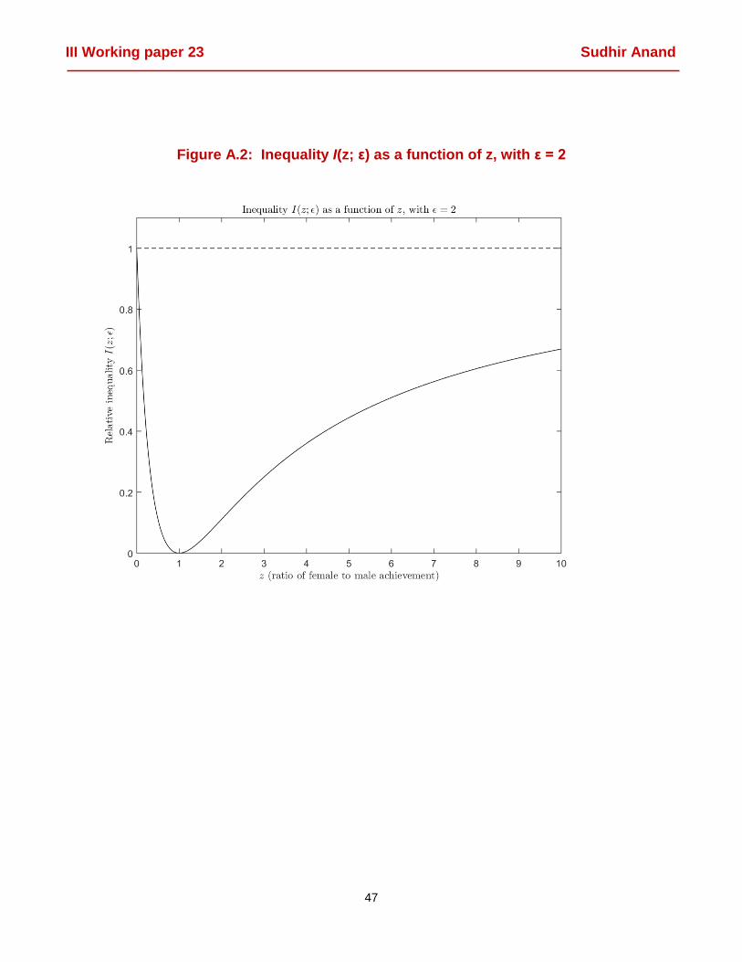
III Working paper 23 Sudhir Anand
47
Figure A.2: Inequality I(z; ε) as a function of z, with ε = 2

III Working paper 23 Sudhir Anand
48
Figure A.3: Inequality A(z) as a function of z

III Working paper 23 Sudhir Anand
49
Annex B
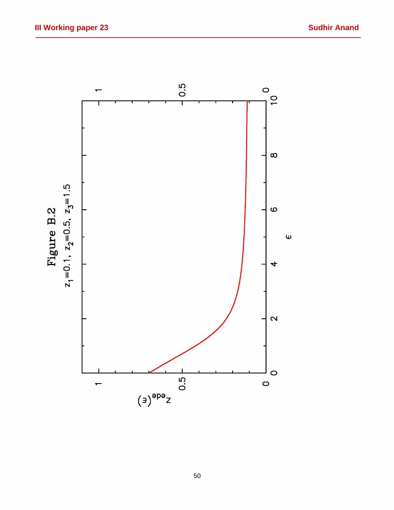
III Working paper 23 Sudhir Anand
50

III Working paper 23 Sudhir Anand
51