Recap: Reasoning Over Time

Stationary Markov models

Hidden Markov models

X2X1 X3 X4 rain sun0.7

0.7

0.3

0.3

X5X2

E1

X1 X3 X4

E2 E3 E4 E5

X E P

rain umbrella 0.9

rain no umbrella 0.1

sun umbrella 0.2

sun no umbrella 0.8This slide deck courtesy of Dan Klein at UC Berkeley

Particle Filtering Sometimes |X| is too big to use 

exact inference |X| may be too big to even store B(X) E.g. X is continuous |X|2 may be too big to do updates

Solution: approximate inference Track samples of X, not all values Samples are called particles Time per step is linear in the number 

of samples But: number needed may be large In memory: list of particles, not 

states

This is how robot localization works in practice

0.0 0.1

0.0 0.0

0.0

0.2

0.0 0.2 0.5

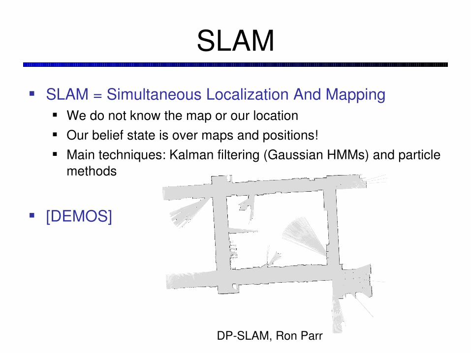
SLAM

SLAM = Simultaneous Localization And Mapping We do not know the map or our location Our belief state is over maps and positions! Main techniques: Kalman filtering (Gaussian HMMs) and particle 

methods

[DEMOS]

DP­SLAM, Ron Parr

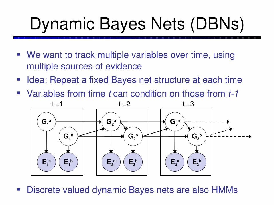
Dynamic Bayes Nets (DBNs)

We want to track multiple variables over time, using multiple sources of evidence

Idea: Repeat a fixed Bayes net structure at each time Variables from time t can condition on those from t­1

Discrete valued dynamic Bayes nets are also HMMs

G1a

E1a E1

b

G1b

G2a

E2a E2

b

G2b

t =1 t =2

G3a

E3a E3

b

G3b

t =3

Exact Inference in DBNs

Variable elimination applies to dynamic Bayes nets Procedure: “unroll” the network for T time steps, then 

eliminate variables until P(XT|e1:T) is computed

Online belief updates: Eliminate all variables from the previous time step; store factors for current time only

5

G1a

E1a E1

b

G1b

G2a

E2a E2

b

G2b

G3a

E3a E3

b

G3b

t =1 t =2 t =3

G3b

DBN Particle Filters

A particle is a complete sample for a time step Initialize: Generate prior samples for the t=1 Bayes net

Example particle: G1a = (3,3) G1

b = (5,3) 

Elapse time: Sample a successor for each particle 

Example successor: G2a = (2,3) G2

b = (6,3)

Observe: Weight each entire sample by the likelihood of the evidence conditioned on the sample Likelihood: P(E1

a |G1a ) * P(E1

b |G1b ) 

Resample: Select prior samples (tuples of values) in proportion to their likelihood 6

Decision Networks

MEU: choose the action which maximizes the expected utility given the evidence

Can directly operationalize this with decision networks Bayes nets with nodes for 

utility and actions Lets us calculate the expected 

utility for each action

New node types: Chance nodes (just like BNs) Actions (rectangles, cannot 

have parents, act as observed evidence)

Utility node (diamond, depends on action and chance nodes)

Weather

Forecast

Umbrella

U

8

Decision Networks

Action selection: Instantiate all 

evidence Set action node(s) 

each possible way Calculate posterior 

for all parents of utility node, given the evidence

Calculate expected utility for each action

Choose maximizing action

Weather

Forecast

Umbrella

U

9

Example: Decision Networks

Weather

Umbrella

U

W P(W)

sun 0.7

rain 0.3

A W U(A,W)

leave sun 100

leave rain 0

take sun 20

take rain 70

Umbrella = leave

Umbrella = take

Optimal decision = leave

Decisions as Outcome Trees

Almost exactly like expectimax / MDPs What’s changed?

11

U(t,s)

Weather Weather

take leave

{}

sun

U(t,r)

rain

U(l,s)

U(l,r)

rainsun

Evidence in Decision Networks

Find P(W|F=bad) Select for evidence

First we join P(W) and P(bad|W)

Then we normalize

Weather

Forecast

W P(W)

sun 0.7

rain 0.3

F P(F|rain)

good 0.1

bad 0.9

F P(F|sun)

good 0.8

bad 0.2

W P(W)

sun 0.7

rain 0.3

W P(F=bad|W)

sun 0.2

rain 0.9

W P(W,F=bad)

sun 0.14

rain 0.27

W P(W | F=bad)

sun 0.34

rain 0.66

12

Umbrella

U

Example: Decision Networks

Weather

Forecastbad=

Umbrella

U

A W U(A,W)

leave sun 100

leave rain 0

take sun 20

take rain 70

W P(W|F=bad)

sun 0.34

rain 0.66

Umbrella = leave

Umbrella = take

Optimal decision = take

13

Decisions as Outcome Trees

14

U(t,s)

W | {b} W | {b}

take leave

sun

U(t,r)

rain

U(l,s)

U(l,r)

rainsun

{b}

Value of Information Idea: compute value of acquiring evidence

Can be done directly from decision network

Example: buying oil drilling rights Two blocks A and B, exactly one has oil, worth k You can drill in one location Prior probabilities 0.5 each, & mutually exclusive Drilling in either A or B has EU = k/2, MEU = k/2

Question: what’s the value of information of O? Value of knowing which of A or B has oil Value is expected gain in MEU from new info Survey may say “oil in a” or “oil in b,” prob 0.5 each If we know OilLoc, MEU is k (either way) Gain in MEU from knowing OilLoc? VPI(OilLoc) = k/2 Fair price of information: k/2

OilLoc

DrillLocU

D O U

a a k

a b 0

b a 0

b b k

O P

a 1/2

b 1/2

15

Value of Information Assume we have evidence E=e.  Value if we act now:

Assume we see that E’ = e’.  Value if we act then:

BUT E’ is a random variable whose value isunknown, so we don’t know what e’ will be

Expected value if E’ is revealed and then we act:

Value of information: how much MEU goes upby revealing E’ first then acting, over acting now:

P(s | e)

{e}a

U{e, e’}a

P(s | e, e’) U

{e}P(e’ | e)

{e, e’}

VPI Example: Weather

Weather

Forecast

Umbrella

U

A W U

leave sun 100

leave rain 0

take sun 20

take rain 70

MEU with no evidence

MEU if forecast is bad

MEU if forecast is good

F P(F)

good 0.59

bad 0.41

Forecast distribution

17

VPI Properties

Nonnegative

Nonadditive – consider, e.g., obtaining Ej twice

Order­independent

18

Quick VPI Questions The soup of the day is either clam chowder or split pea, 

but you wouldn’t order either one.  What’s the value of knowing which it is?

There are two kinds of plastic forks at a picnic.  One kind is slightly sturdier.  What’s the value of knowing which?

You’re playing the lottery.  The prize will be $0 or $100.  You can play any number between 1 and 100 (chance of winning is 1%).  What is the value of knowing the winning number?

POMDPs MDPs have:

States S Actions A Transition fn P(s’|s,a) (or T(s,a,s’)) Rewards R(s,a,s’)

POMDPs add: Observations O Observation function P(o|s) (or O(s,o))

POMDPs are MDPs over beliefstates b (distributions over S)

We’ll be able to say more in a few lectures

as

s, a

s,a,s’ s

’

ab

b, a

     ob’

20

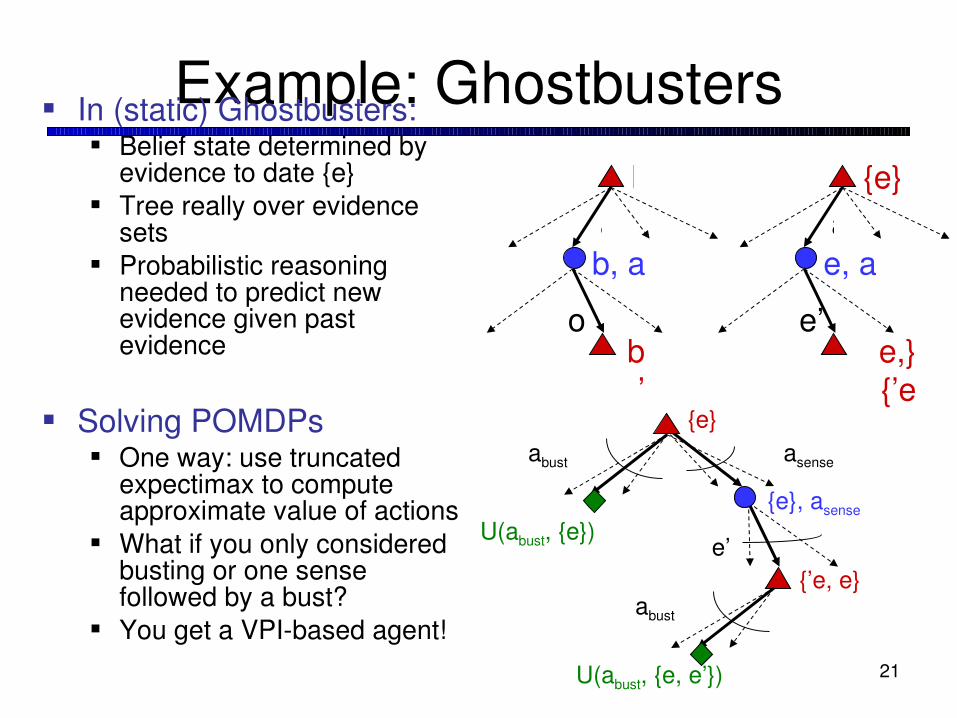
Example: Ghostbusters In (static) Ghostbusters:

Belief state determined by evidence to date {e}

Tree really over evidence sets

Probabilistic reasoning needed to predict new evidence given past evidence

Solving POMDPs One way: use truncated 

expectimax to compute approximate value of actions

What if you only considered busting or one sense followed by a bust?

You get a VPI­based agent!

a{e}

e, a

    e’e,}{’e

ab

b, a

    ob’

abust

{e}

{e}, asense

      e’{’e, e}

asense

U(abust, {e})

abust

U(abust, {e, e’}) 21

More Generally General solutions map belief 

functions to actions Can divide regions of belief space 

(set of belief functions) into policy regions (gets complex quickly)

Can build approximate policies using discretization methods

Can factor belief functions in various ways

Overall, POMDPs are very (actually PSACE­) hard

Most real problems are POMDPs, but we can rarely solve then in general!

22

VPI Example: Ghostbusters

T B G P(T,B,G)+t +b +g 0.16

+t +b ¬g 0.16

+t ¬b +g 0.24

+t ¬b ¬g 0.04

¬t +b +g 0.04

¬t +b ¬g 0.24

¬t ¬b +g 0.06

¬t ¬b ¬g 0.06

Reminder: ghost is hidden, sensors are noisy

T: Top square is redB: Bottom square is redG: Ghost is in the top

Sensor model:

P( +t | +g ) = 0.8P( +t | ¬g ) = 0.4P( +b | +g) = 0.4P( +b | ¬g ) = 0.8

Joint Distribution

[Demo]

VPI Example: Ghostbusters

T B G P(T,B,G)+t +b +g 0.16

+t +b ¬g 0.16

+t ¬b +g 0.24

+t ¬b ¬g 0.04

¬t +b +g 0.04

¬t +b ¬g 0.24

¬t ¬b +g 0.06

¬t ¬b ¬g 0.06

Utility of bust is 2, no bust is 0

Q1: What’s the value of knowing T if I know nothing?

Q1’: EP(T)[MEU(t) – MEU()]

Q2: What’s the value of knowing B if I already know that T is true (red)?

Q2’: EP(B|t)[MEU(t,b) – MEU(t)]

How low can the value of information ever be?

Joint Distribution

[Demo]

Conditioning on Action Nodes

An action node can be a parent of a chance node

Chance node conditions on the outcome of the action

Action nodes are like observed variables in a Bayes’ net, except we max over their values

25

S’

A

U

S

T(s,a,s’) R(s,a,s’)

Speech and Language Speech technologies

Automatic speech recognition (ASR) Text­to­speech synthesis (TTS) Dialog systems

Language processing technologies Machine translation

Information extraction Web search, question answering Text classification, spam filtering, etc…

Digitizing Speech

27

Speech in an Hour

Speech input is an acoustic wave form

   s             p       ee         ch           l     a          b

Graphs from Simon Arnfield’s web tutorial on speech, Sheffield:

http://www.psyc.leeds.ac.uk/research/cogn/speech/tutorial/

“l” to “a”transition:

28

Frequency gives pitch; amplitude gives volume sampling at ~8 kHz phone, ~16 kHz mic (kHz=1000 cycles/sec)

Fourier transform of wave displayed as a spectrogram darkness indicates energy at each frequency

   s             p       ee         ch           l     a          b

frequ

ency

ampl

itude

Spectral Analysis

29

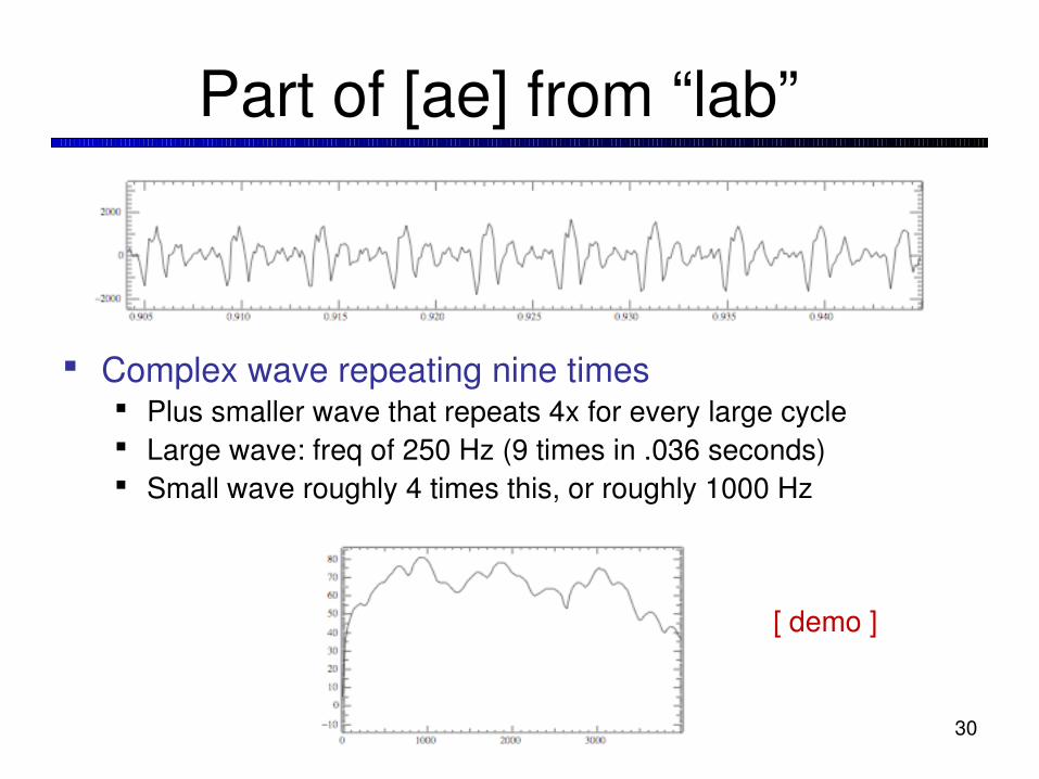
Part of [ae] from “lab”

Complex wave repeating nine times Plus smaller wave that repeats 4x for every large cycle Large wave: freq of 250 Hz (9 times in .036 seconds) Small wave roughly 4 times this, or roughly 1000 Hz

30

[ demo ]

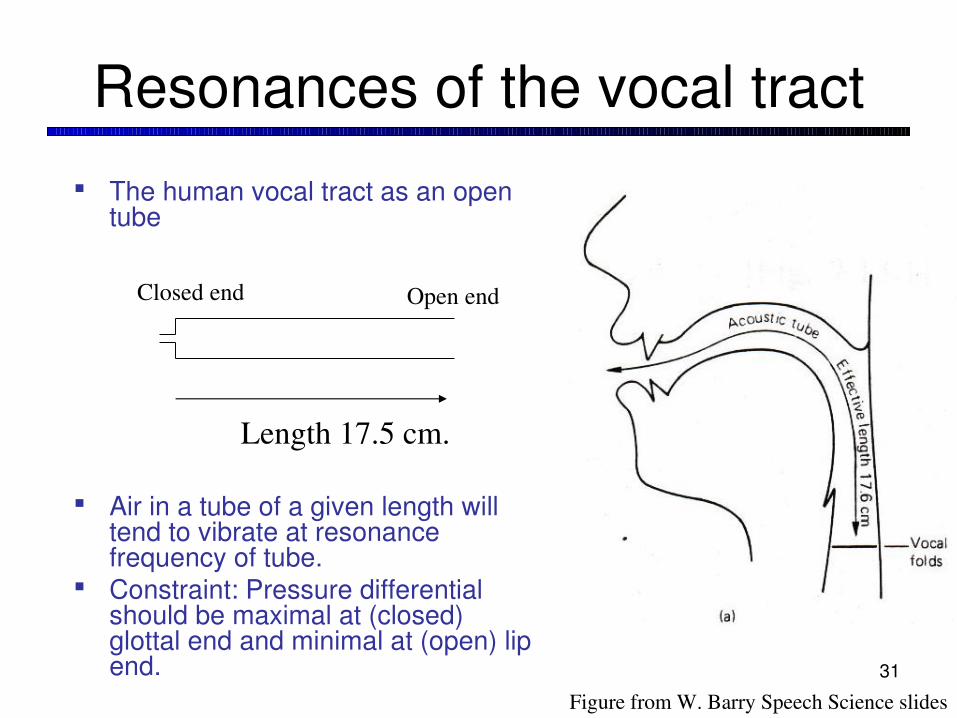
Resonances of the vocal tract

The human vocal tract as an open tube

Air in a tube of a given length will tend to vibrate at resonance frequency of tube. 

Constraint: Pressure differential should be maximal at (closed) glottal end and minimal at (open) lip end.

Closed end Open end

Length 17.5 cm.

Figure from W. Barry Speech Science slides31

FromMarkLiberman’swebsite

32

[ demo ]

Figures from Ratree Wayland

Vowel [i] sung at successively higher pitches 

A3

A4

A2

C4 (middle C)

C3

F#3

F#2

Acoustic Feature Sequence Time slices are translated into acoustic feature 

vectors (~39 real numbers per slice)

These are the observations, now we need the hidden states X

frequ

ency

……………………………………………..e12e13e14e15e16………..

34

State Space

P(E|X) encodes which acoustic vectors are appropriate for each phoneme (each kind of sound)

P(X|X’) encodes how sounds can be strung together  We will have one state for each sound in each word From some state x, can only:

Stay in the same state (e.g. speaking slowly) Move to the next position in the word At the end of the word, move to the start of the next word

We build a little state graph for each word and chain them together to form our state space X

35

HMMs for Speech

36

Transitions with Bigrams

Figure from Huang et al page 618

198015222 the first194623024 the same168504105 the following158562063 the world…14112454 the door­­­­­­­­­­­­­­­­­23135851162 the *

Trai

ning

 Cou

nts

Decoding

While there are some practical issues, finding the words given the acoustics is an HMM inference problem

We want to know which state sequence x1:T is most likely given the evidence e1:T:

From the sequence x, we can simply read off the words38

End of Part II!

Now we’re done with our unit on probabilistic reasoning

Last part of class: machine learning

39