really uncertain business cycles - nicholas bloom · uncertain business cycles 1033 figure 2.—the...

http://www.econometricsociety.org/

Econometrica, Vol. 86, No. 3 (May, 2018), 1031–1065

REALLY UNCERTAIN BUSINESS CYCLES

NICHOLAS BLOOMDept. of Economics, Stanford University

MAX FLOETOTTOMcKinsey & Company

NIR JAIMOVICHDept. of Economics, University of Zurich

ITAY SAPORTA-EKSTENDept. of Economics, Tel Aviv University and Dept. Economics, University College London

STEPHEN J. TERRYDept. of Economics, Boston University

The copyright to this Article is held by the Econometric Society. It may be downloaded, printed and re-produced only for educational or research purposes, including use in course packs. No downloading orcopying may be done for any commercial purpose without the explicit permission of the Econometric So-ciety. For such commercial purposes contact the Office of the Econometric Society (contact informationmay be found at the website http://www.econometricsociety.org or in the back cover of Econometrica).This statement must be included on all copies of this Article that are made available electronically or inany other format.


Econometrica, Vol. 86, No. 3 (May, 2018), 1031–1065

REALLY UNCERTAIN BUSINESS CYCLES

NICHOLAS BLOOMDept. of Economics, Stanford University

MAX FLOETOTTOMcKinsey & Company

NIR JAIMOVICHDept. of Economics, University of Zurich

ITAY SAPORTA-EKSTENDept. of Economics, Tel Aviv University and Dept. Economics, University College London

STEPHEN J. TERRYDept. of Economics, Boston University

We investigate the role of uncertainty in business cycles. First, we demonstrate thatmicroeconomic uncertainty rises sharply during recessions, including during the GreatRecession of 2007–2009. Second, we show that uncertainty shocks can generate dropsin gross domestic product of around 2.5% in a dynamic stochastic general equilibriummodel with heterogeneous firms. However, we also find that uncertainty shocks needto be supplemented by first-moment shocks to fit consumption over the cycle. So ourdata and simulations suggest recessions are best modelled as being driven by shockswith a negative first moment and a positive second moment. Finally, we show that in-creased uncertainty can make first-moment policies, like wage subsidies, temporarilyless effective because firms become more cautious in responding to price changes.

KEYWORDS: Uncertainty, adjustment costs, business cycles.

1. INTRODUCTION

UNCERTAINTY has received substantial attention recently. For example, the Federal OpenMarket Committee minutes repeatedly emphasize uncertainty as a key factor in the 2001and 2007–2009 recessions. This paper seeks to evaluate the role of uncertainty for busi-ness cycles in two parts. In the first part, we develop new empirical measures of uncer-tainty using detailed Census microdata from 1972–2011 and we highlight three mainresults. First, the dispersion of plant-level innovations to their total factor productivity(TFP) is strongly countercyclical, rising steeply in recessions. For example, Figure 1 showsthe dispersion of TFP shocks for a balanced panel of plants during the 2 years beforethe Great Recession (2005–2006) and 2 years during the recession (2008–2009). We find

Nicholas Bloom: [email protected] Floetotto: [email protected] Jaimovich: [email protected] Saporta-Eksten: [email protected] J. Terry: [email protected] opinions and conclusions expressed herein are those of the authors and do not necessarily represent

the views of the U.S. Census Bureau. All results have been reviewed to ensure that no confidential informationis disclosed. We thank our editor Lars Hansen, our anonymous referees, our formal discussants Sami Alpanda,Eduardo Engel, Frank Smets, Eric Swanson, and Iván Alfaro, as well as Angela Andrus at the RDC andnumerous seminar audiences for comments.

© 2018 The Econometric Society https://doi.org/10.3982/ECTA10927


mailto:[email protected]






https://doi.org/10.3982/ECTA10927

1032 BLOOM ET AL.

FIGURE 1.—The variance of establishment-level TFP shocks increased by 76% in the Great Recession.Notes: Constructed from the Census of Manufactures and the Annual Survey of Manufactures using a bal-anced panel of 15,752 establishments active in 2005–2006 and 2008–2009. TFP Shocks are defined as residualsfrom a plant-level log(TFP) AR(1) regression that also includes plant and year fixed effects. Moments ofthe distribution for non-recession (recession) years are: mean 0 (−0�166), variance 0.198 (0.349), coefficientof skewness −1�060 (−1�340) and kurtosis 15.01 (11.96). The year 2007 is omitted because according to theNBER the recession began in 12/2007, so 2007 is not a clean “before” or “during” recession year.

that plant-level TFP shocks increased in variance by 76% during the recession. Similarly,Figure 2 shows that the dispersion of output growth for these same establishments in-creased even more, rising by a striking 152% during the recession. Thus, as Figures 1 and2 suggest, recessions appear to be characterized by a negative first-moment and a positivesecond-moment shock to the establishment-level driving processes.

Our second empirical finding is that uncertainty is also strongly countercyclical at theindustry level. That is, at the Standard Industrial Classification (SIC) four-digit industrylevel, the yearly growth rate of output is negatively correlated with the dispersion of TFPshocks to establishments within the industry. Hence, both at the industry and at the ag-gregate level, periods of low growth rates of output are also characterized by increasedcross-sectional dispersion of TFP shocks.

Our third empirical finding is that for plants owned by publicly traded Compustat par-ent firms, the size of their plant-level TFP shocks is positively correlated with their par-ents’ daily stock returns. Hence, daily stock returns volatility—a popular high-frequencyfinancial measure of uncertainty that also rises in recessions—is tightly linked to the sizeof yearly plant TFP shocks.

Given this empirical evidence that uncertainty appears to rise sharply in recessions, inthe second part of the paper we build a dynamic stochastic general equilibrium (DSGE)model. Various features of the model are specified to conform as closely as possible to thestandard frictionless real business cycle (RBC) model as this greatly simplifies compari-son with existing work. We deviate from this benchmark in three ways. First, uncertaintyis time-varying, so the model includes shocks to both the level of technology (the firstmoment) and its variance (the second moment) at both the microeconomic and macroe-conomic levels. Second, there are heterogeneous firms that are subject to idiosyncraticshocks. Third, the model contains nonconvex adjustment costs in both capital and labor.

UNCERTAIN BUSINESS CYCLES 1033

FIGURE 2.—The variance of establishment-level sales growth rates increased by 152% in the Great Reces-sion. Notes: Constructed from the Census of Manufactures and the Annual Survey of Manufactures using abalanced panel of 15,752 establishments active in 2005–2006 and 2008–2009. Moments of the distribution fornon-recession (recession) years are: mean 0.026 (−0�191), variance 0.052 (0.131), coefficient of skewness 0.164(−0�330) and kurtosis 13.07 (7.66). The year 2007 is omitted because according to the NBER the recessionbegan in 12/2007, so 2007 is not a clean “before” or “during” recession year.

The nonconvexities together with time variation in uncertainty imply that firms becomemore cautious in investing and hiring when uncertainty increases.

The model is numerically solved and estimated using macro- and plant-level data via asimulated method of moments (SMM) approach. Our SMM parameter estimates suggestthat micro- and macro-uncertainty increase by around threefold during recessions.

Simulations of the model allow us to study its response to an uncertainty shock. In-creased uncertainty makes it optimal for firms to wait, leading to significant falls in hir-ing, investment, and output. In our model, overall, uncertainty shocks generate a drop ingross domestic product (GDP) of around 2.5%. Moreover, the increased uncertainty re-duces productivity growth. This reduction occurs because uncertainty reduces the degreeof reallocation in the economy since productive plants pause expanding and unproduc-tive plants pause contracting. The importance of reallocation for aggregate productivitygrowth matches empirical evidence in the United States. See, for example, Foster, Halti-wanger, and Krizan (2000, 2006), who report that reallocation broadly defined accountsfor around 50% of manufacturing and 80% of retail productivity growth in the UnitedStates.

We then build on our theoretical model to investigate the effects of uncertainty onpolicy effectiveness. We use a simple illustrative example to show how time-varying un-certainty initially dampens the effect of an expansionary policy. The key to this policyineffectiveness is that a rise in uncertainty makes firms cautious in responding to anystimulus.

Our work is related to several strands in the literature. First, we add to the extensiveliterature building on the DSGE framework that studies the role of TFP shocks in caus-ing business cycles. In this literature, recessions are generally caused by large negativetechnology shocks (e.g., King and Rebelo (1999)). The reliance on negative technologyshocks has proven to be controversial, as it suggests that recessions are times of techno-

1034 BLOOM ET AL.

logical regress. As discussed above, our work provides a rationale for at least some portionof variation in measured productivity. Countercyclical increases in uncertainty lead to afreeze in economic activity, substantially lowering productivity growth during recessions.

Second, the paper relates to the literature on investment under uncertainty. A rapidlygrowing body of work has shown that uncertainty can directly influence firm-level invest-ment and employment in the presence of adjustment costs. Recently, the literature hasstarted to focus on stochastic volatility and its impacts on the economy.1 Finally, the pa-per also builds upon a recent literature that studies the role of microeconomic rigiditiesin general equilibrium macromodels.2

The remainder of this paper is organized as follows. Section 2 discusses the empiri-cal behavior of uncertainty over the business cycle. In Section 3, we formally present theDSGE model, define the recursive equilibrium, and present our nonlinear solution al-gorithm. We discuss the estimation of parameters governing the uncertainty process inSection 4, while in Section 5, we study the impact of uncertainty shocks on the aggre-gate economy. Section 6 studies the implications for government policy in the presenceof time-varying uncertainty. Section 7 concludes. Appendixes in the Supplementary Ma-terial (Bloom, Floetotto, Jaimovich, Saporta-Eksten, and Terry (2018)) include details onthe data (Appendix A), model solution (Appendix B), estimation (Appendix C), and abenchmark representative agent model (Appendix D).

2. MEASURING UNCERTAINTY OVER THE BUSINESS CYCLE

Before presenting our empirical results, it is useful to briefly discuss what we mean bytime-varying uncertainty in the context of our model.

We assume that a firm, indexed by j, produces output in period t according to theproduction function

yj�t =Atzj�tf (kj�t� nj�t)� (1)

where kt�j and nt�j denote idiosyncratic capital and labor employed by the firm. Each firm’sproductivity is a product of two separate processes: an aggregate component, At , and anidiosyncratic component, zj�t .

We assume that the aggregate and idiosyncratic components of business conditions fol-low autoregressive (AR) processes:

log(At)= ρA log(At−1)+ σAt−1εt� (2)

log(zj�t)= ρZ log(zj�t−1)+ σZt−1εj�t � (3)

1For a focus on the firm level, see Bernanke (1983), Romer (1990), Bertola and Caballero (1994), Dixitand Pindyck (1994), Abel and Eberly (1996), Hassler (1996), and Caballero and Engel (1999). For a macro-focus, see Bloom’s (2009) partial equilibrium model with stochastic volatility, Fernandez-Villaverde, Guerron-Quintana, Rubio-Ramirez, and Uribe’s (2011) paper on uncertainty and real exchange rates, Kehrig’s (2015)paper on countercyclical productivity dispersion, Christiano, Motto, and Rostagno’s (2014), Arellano, Bai, andKehoe’s (2012), and Gilchrist, Sim, and Zakrajsek’s (2014) papers on uncertainty shocks in models with finan-cial constraints, Basu and Bundick’s (2016) paper on uncertainty shocks in a new-Keynesian model, Fernandez-Villaverde, Guerron-Quintana, Kuester, and Rubio-Ramirez’s (2015) paper on fiscal policy uncertainty, andBachmann and Bayer’s (2013, 2014) papers on microlevel uncertainty with capital adjustment costs.

2See, for example, Hopenhayn and Rogerson (1993), Thomas (2002), Veracierto (2002), Gourio andKashyap (2007), Khan and Thomas (2008, 2013), Bachmann, Caballero, and Engel (2013), House (2014),or Winberry (2016).


We allow the variance of innovations, σAt and σZt , to move over time according to two-state Markov chains, generating periods of low and high macro- and micro-uncertainty.

There are two assumptions embedded in this formulation. First, the volatility in theidiosyncratic component, zj�t , implies that productivity dispersion across firms is time-varying, while volatility in the aggregate component,At , implies that all firms are affectedby more volatile shocks. Second, given the timing assumption in (2) and (3), firms learnin advance that the distribution of shocks from which they will draw in the next period ischanging. This timing assumption captures the notion of uncertainty that firms face aboutfuture business conditions.

These two shocks are driven by different statistics. Volatility in zj�t implies that cross-sectional dispersion-based measures of firm performance (output, sales, stock market re-turns, etc.) are time-varying, while volatility in At induces higher variability in aggregatevariables like GDP growth and the Standard and Poor’s 500 index. Next we turn to ourcross-sectional and macroeconomic uncertainty measures, detailing how both appear torise in recessions.

2.1. Microeconomic Uncertainty Over the Business Cycle

In this section we present a set of results showing that shocks at the establishment-level,firm-level, and industry-level all increase in variance during recessions. In our model inSection 3 we focus on units of production, ignoring multi-establishment firms or industry-level shocks to reduce computational burden. Nevertheless, we present data at these threedifferent levels to demonstrate the generality of the increase in idiosyncratic shocks dur-ing recessions.

Our first set of measures comes from the Census panel of manufacturing establish-ments. In summary, with extensive details in Appendix A, this data set contains de-tailed output and input data on over 50,000 establishments from 1972 to 2011. We focuson the subset of 15,673 establishments with 25+ years of data to ensure that compo-sitional changes do not bias our results, generating a sample of almost half a millionestablishment–year observations.

To measure uncertainty, we first calculate establishment-level TFP (zj�t) using the stan-dard approach from Foster, Haltiwanger, and Krizan (2000). We then define TFP shocks(ej�t) as the residual from the first-order autoregressive equation for establishment-levellog TFP,

log(zj�t)= ρ log(zj�t−1)+μj + λt + ej�t� (4)

where μj is an establishment-level fixed effect (to control for permanent establishment-level differences) and λt is a year fixed effect (to control for cyclical shocks). Since thisresidual also contains plant-level demand shocks that are not controlled for by four-digitprice deflators (see Foster, Haltiwanger, and Syverson (2008)), our revenue-based mea-sure will combine both TFP and demand shocks.

Finally, we define microeconomic uncertainty, σZt−1, as the cross-sectional dispersion ofej�t calculated on a yearly basis. In Figure 3, we depict the interquartile range (IQR) of thisTFP shock within each year. As Figure 3 shows, the series exhibits a clearly countercyclicalbehavior. This is particularly striking for the recent Great Recession of 2007–2009, whichdisplays the highest value of TFP dispersion since the series began in 1972.

Table I more systematically evaluates the relationship between the dispersion of TFPshocks and recessions. In column 1, we regress the cross-sectional standard deviation(S.D.) of establishment TFP shocks on an indicator for the number of quarters in a re-cession during that year. So, for example, this variable has a value of 0.25 in 2007 as the

1036 BLOOM ET AL.

FIGURE 3.—TFP “shocks” are more dispersed in recessions. Notes: Constructed from the Census of Man-ufactures and the Annual Survey of Manufactures establishments, using establishments with 25+ years toaddress sample selection. Grey shaded columns are the share of quarters in recession within a year.

recession started in quarter IV, and values of 1 and 0.5 in 2008 and 2009, respectively, asthe recession continued until quarter II in 2009. We find a coefficient of 0.064, which ishighly significant (a t-statistic of 6.9). Given that the mean of the S.D. of establishmentTFP shocks is 0.503, a year in recession is associated with a 13% increase in the dispersionof TFP shocks. In the bottom panel, we report that this S.D. of establishment TFP shocksalso has a highly significant correlation with GDP growth of −0�45.

Our finding here of countercyclical dispersion of microlevel outcomes mirrors a rangeof other recent papers such as Bachmann and Bayer (2014) in German data, Kehrig(2015) in a similar sample of U.S. Census data, or Jurado, Ludvigson, and Ng (2014),Vavra (2014), and Berger and Vavra (2015) for different samples of U.S. firms. A num-ber of these papers build alternative theories or interpretations of such patterns in themicrodata qualitatively distinct from our own, but the core empirical regularity of coun-tercyclical microlevel dispersion is remarkably robust.

In columns 2 and 3, we examine the coefficient of skewness and kurtosis of TFP shocksover the cycle and, interestingly, find no significant correlations.3 This suggests that reces-sions can be characterized at the microeconomic level as a negative first-moment shockplus a positive second-moment shock. In column 4, we use an outlier-robust measure ofcross-sectional dispersion, which is the IQR range of TFP shocks, and again find this risessignificantly in recessions. The point estimate on recession of 0.061 implies an increase ofover 15% in the IQR of TFP shocks in a recession year.4 In column 5, as another robust-

3This lack of significant correlation was robust in a number of experiments we ran. For example, if we dropthe time trend and Census survey year controls, the result in column 1 on the standard deviation remains highlysignificant at 0.062 (0.020), while the results in columns 2 and 3 on skewness and kurtosis remain insignificantat −0�250 (0.243) and −0�771 (2.755). We also experimented with changing the establishment selection rules(keeping those with 2+ or 38+ years rather than 25+ years) and again found the results robust, as shownin Appendix Table A1. Interestingly, Guvenen, Ozkan, and Song (2014) find an increase in left-skewness forpersonal income growth during recessions, which may be absent in plant data because large negative drawslead plants to exit. Because the drop in the left tail is the key driver of recessions in our model (the “bad newsprinciple” highlighted by Bernanke (1983)), this distinction is relatively unimportant.

4While 15% is a large increase in dispersion, it still greatly understates the increase in uncertainty in reces-sion, because a large share of the dispersion of TFP is associated with measurement error. We formally address

UN

CE

RTA

INB

USIN

ESS

CY

CL

ES

1037

TABLE I

UNCERTAINTY IS HIGHER DURING RECESSIONSa

(1) (2) (3) (4) (5) (6) (7) (8)

Dependent S.D. of log(TFP) Skewness of Kurtosis of IQR of log(TFP) IQR of IQR of IQR of IQR of industrialvariable: shock log(TFP) log(TFP) shock output growth sales growth stock returns prod. growth

shock shockSample: Plants Plants Plants Plants Plants Public firms Public firms Industries

(manufact.) (manufact.) (manufact.) (manufact.) (manufact.) (all sectors) (all sectors) (manufact.)

Recession 0.064∗∗∗ −0.248 −1.334 0.061∗∗∗ 0.077∗∗∗ 0.032∗∗∗ 0.025∗∗∗ 0.044∗∗∗

(0.009) (0.191) (1.994) (0.019) (0.019) (0.007) (0.003) (0.004)

Mean of dep. var. 0.503 −1.525 20.293 0.395 0.196 0.186 0.104 0.101Corr. GDP growth −0.450∗∗∗ 0.143 0.044 −0.444∗∗∗ −0.566∗∗∗ −0.275∗∗∗ −0.297∗∗∗ −0.335∗∗∗

Frequency Annual Annual Annual Annual Annual Quarterly Monthly MonthlyYears 1972–2011 1972–2011 1972–2011 1972–2011 1972–2011 1962:1–2010:3 1960–2010 1972–2010Observations 39 39 39 39 39 191 609 455Underlying sample 461,232 461,232 461,232 461,232 461,232 320,306 931,143 70,487

aEach column reports a time-series ordinary least squares (OLS) regression point estimate (and standard error below in parentheses) of a measure of uncertainty on a recession indicator. Therecession indicator is the share of quarters in that year in a recession in columns 1–5, whether that quarter was in a recession in column 6, and whether the month was in recession in columns 7 and 8.Recessions are defined using the National Bureau of Economic Research (NBER) data. In the bottom panel we report the mean of the dependent variable and its correlation with real GDP growth. Incolumns 1–5, the sample is the population of manufacturing establishments with 25 years or more of observations in the Annual Survey of Manufactures (ASM) or Census of Manufactures (CM) surveybetween 1972 and 2009, which contains data on 15,673 establishments across 40 years of data (one more year than the 39 years of regression data since we need lagged TFP to generate a TFP shockmeasure). We include plants with 25+ years to reduce concerns over changing samples. In column 1, the dependent variable is the cross-sectional standard deviation (S.D.) of the establishment-levelshock to total factor productivity (TFP). This shock is calculated as the residual from the regression of log(TFP) at year t + 1 on its lagged value (year t), a full set of year dummies, and establishmentfixed effects. In column 2, we use the cross-sectional coefficient of skewness of the TFP shock, in column 3, the cross-sectional coefficient of kurtosis, and in column 4, the cross-sectional interquartilerange of this TFP shock as an outlier robust measure. In column 5, the dependent variable is the interquartile range of plants’ sales growth. In column 6, the dependent variable is the interquartilerange of firms’ sales growth by quarter for all public firms with 25 years (100 quarters) or more in Compustat between 1962 and 2010. In column 7, the dependent variable is the within firm-quarterinterquartile range of firms’ monthly stock returns for all public firms with 25 years (300 months) or more in Center for Research in Security Prices (CRSP) between 1960 and 2010. Finally, in column8, the dependent variable is the interquartile range of industrial production growth by month for manufacturing industries from the Federal Reserve Board’s monthly industrial production database.All regressions include a time trend and for columns 1–5 Census year dummies (for Census year and for three lags). Robust standard errors are applied in all columns to control for any potentialserial correlation. ∗∗∗ denotes 1% significance, ∗∗ denotes 5% significance, and ∗ denotes 10% significance. Results are also robust to using Newey–West corrections for the standard errors. Data areavailable at http://www.stanford.edu/~nbloom/RUBC.zip.

http://www.stanford.edu/~nbloom/RUBC.zip

1038 BLOOM ET AL.

ness test, we use plant-level output growth, rather than TFP shocks, and find a significantrise in recessions. We also run a range of other experiments on different indicators, mea-sures of TFP, and samples, and always find that dispersion rises significantly in recessions.5For example, Figure A1 plots the correlation of plant TFP rankings between consecutiveyears. This shows that during recessions these rankings churn much more, as increasedmicroeconomic variance leads plants to change their position within their industry-levelTFP rankings more rapidly.

In column 6, we use a different data set that is the sample of all Compustat firms with25+ years of data. This has the downside of being a much smaller selected sample con-taining only 2465 publicly quoted firms, but spanning all sectors of the economy, andproviding quarterly sales observations going back to 1962. We find that the quarterly dis-persion of sales growth in this Compustat sample is also significantly higher in recessions.

One important caveat when using the variance of productivity “shocks” to measure un-certainty is that the residual ej�t is a productivity shock only in the sense that it is unfore-casted by the regression equation (4), rather than unforecasted by the establishment. Weaddress this concern in two ways. First, in column 7 we examine the cross-sectional spreadof stock returns, which reflects the volatility of news about firm performance, and againfind this is countercyclical, echoing the prior results in Campbell, Lettau, Malkiel, andXu (2001). In fact, as we discuss below in Table III, we also find that establishment-levelshocks to TFP are significantly correlated to their parent’s stock returns, so that at leastpart of these establishment TFP shocks are new information to the market. Furthermore,to remove the forecastable component of stock returns, we repeated the specification incolumn 7 by first removing the quarter by firm mean of firm returns. This controls for anyquarterly factors—like size, market/book value, research and development (R&D) in-tensity, and leverage—that may influence expected stock returns (e.g., Bekaert, Hodrick,and Zhang (2012)), although of course the influence of common factors that may vary ata higher frequency within the quarter may remain. The coefficient (standard error) onrecession in these regressions is 0.019 (0.003), similar to the results obtained in column 7.

Second, we extend the TFP forecast regressions (4) to include additional observablesthat are likely to be informative about future TFP changes. Adding these in the regressionaccounts for at least some of the superior information that the establishment might haveover the econometrician, helping us to back out true shocks to TFP from the perspec-tive of the establishments. Figure 4 reports the IQR of the TFP shocks for the baselineforecast regression, as well as for three other dispersion measures, where we sequentiallyadd more variables to the forecasting regressions that are used to recover TFP shocks.First we add two extra lags in levels and polynomials of TFP, next we also include lagsand polynomials of investment, and finally we include lags and polynomials of multipleinputs including employment, energy, and materials expenditure. As is clear from the fig-ure, even when forward looking establishment choices for investment and employmentare included, the overall cyclical patterns of uncertainty are almost unchanged.

that in our SMM estimation framework. See Section 4.2 for estimates of the underlying increase in uncertaintyin recession and see Appendix C for details.

5For example, the IQR of employment growth rates has a point estimate (standard error) of 0.051 (0.012),the IQR of TFP shocks measured using an industry-by-industry forecasting equation version of (4) has a pointestimate (standard error) of 0.064 (0.019), using 2+ year samples for the S.D. of TFP shocks, we find a pointestimate (standard error) of 0.046 (0.014), and using a balanced panel of 38+ year establishments, we finda point estimate (standard error) of 0.075 (0.015). Finally, the IQR of TFP shocks measured after removingfirm–year means and then applying (4) has a point estimate (standard error) of 0.028 (0.011), so that dispersionof productivity shocks even across plants within firms rises within recessions.


FIGURE 4.—Robustness test: different measures of TFP “shocks” are all more dispersed in recessions.Notes: Constructed from the Census of Manufactures and the Annual Survey of Manufactures establishments,using establishments with 25+ years to address sample selection. Grey shaded columns are share of quarters inrecession within a year. The four lines are: Baseline: Interquartile Range of plant TFP “shocks” (as in Figure 3).Add polynomials in TFP: includes the first, second and third lags of log TFP, and their degree 5 polynomialsin the AR regression which is used to recover TFP shocks. Add investment: includes all the controls from theprevious specification plus the first, second and third lags of investment rate, and their degree 5 polynomials.Add emp, sales and materials: includes all the controls from the previous specification plus the second and thirdlags of log employment, log sales, and log materials, as well as their degree 5 polynomials.

Finally, in column 8, we examine another measure of uncertainty, which is the cross-sectional spread of industry-level output growth rates, finding again that this is stronglycountercyclical.

Hence, in summary plant-level (columns 1–5), firm-level (columns 6 and 7), andindustry-level (column 8) measures of volatility and uncertainty all appear to be stronglycountercyclical, suggesting that microeconomic uncertainty rises in recessions at all levels.

2.2. Industry Business Cycles and Uncertainty

In Table II, we report another set of results that disaggregate down to the industrylevel, finding a very similar result that uncertainty is significantly higher during periodsof slower growth. To do this, we exploit the size of our Census data set to examine thedispersion of productivity shocks within each SIC four-digit industry–year cell. The sizeof the Census data set means that it has a mean (median) of 27.1 (17) establishments perSIC four-digit industry–year cell, which enables us to examine the link between within-industry dispersion of establishment TFP shocks and industry growth.

Table II displays a series of industry panel regressions in which our dependent variableis the IQR of TFP shocks for all establishments in each industry (i)–year (t) cell. Theregression specification that we run is

IQRi�t = ai + bt + γyi�t �The explanatory variable in column (1) (yi�t) is the median growth rate of output be-tween t and t + 1 in the industry–year cell, with a full set of industry (ai) and year (bt)

1040B

LO

OM

ET

AL

.

TABLE II

UNCERTAINTY IS ALSO ROBUSTLY HIGHER AT THE INDUSTRY LEVEL DURING INDUSTRY “RECESSIONS”a

(1) (2) (3) (4) (5) (6) (7) (8) (9)

Dependent variable: IQR of establishment TFP shocks within each industry–year cellSpecification: Baseline Median IQR of Median IQR of Median IQR of IQR of Industry

industry industry industry industry industry industry industry geographicoutput output establishment establishment capital/labor capital/labor TFP spread spreadgrowth growth size size ratio ratio

Industry output growth −0.132∗∗∗ −0.142∗∗∗ −0.176∗∗∗ −0.119∗∗∗ −0.116∗∗∗ −0.111∗∗∗ −0.111∗∗∗ −0.191∗∗∗ −0.133∗∗∗

(0.021) (0.021) (0.047) (0.024) (0.022) (0.034) (0.030) (0.041) (0.028)

Interaction of industry 0.822 0.882 −0.032 −0.033 −0.197 −0.265 0.123 0.007output growth with (0.630) (0.996) (0.038) (0.026) (0.292) (0.330) (0.084) (0.122)the variable inspecification row

Years 1972–2009 1972–2009 1972–2009 1972–2009 1972–2009 1972–2009 1972–2009 1972–2009 1972–2009Observations 16,451 16,451 16,451 16,451 16,451 16,451 16,451 16,451 16,451Underlying sample 446,051 446,051 446,051 446,051 446,051 446,051 446,051 446,051 446,051

aEach column reports the results from an industry-by-year OLS panel regression, including a full set of industry and year fixed effects. The dependent variable in every column is the interquartilerange (IQR) of establishment-level TFP shocks within each SIC four-digit industry–year cell. The regression sample is the 16,451 industry–year cells of the population of manufacturing establishmentswith 25 years or more of observations in the ASM or CM survey between 1972 and 2009 (which contains 446,051 underlying establishment years of data). These industry–year cells are weighted in theregression by the number of establishment observations within that cell, with the mean and median number of establishments per industry–year cell equal to 27.1 and 17, respectively. The TFP shockis calculated as the residual from the regression of log(TFP) at year t + 1 on its lagged value (year t), a full set of year dummies, and establishment fixed effects. In column 1, the explanatory variableis the median of the establishment-level output growth in that industry–year. In columns 2–9, a second variable is also included that is an interaction of that explanatory variable with an industry-levelcharacteristic. In columns 2 and 3, this is the median and IQR of industry-level output growth, in columns 4 and 5 this is the median and IQR of industry-level establishment size in employees, incolumns 6 and 7, this is the median and IQR of industry-level capital/labor ratios, in column 8 this is the IQR of industry-level TFP levels (note the mean is zero by construction), while finally incolumn 9, this interaction is the dispersion of industry-level concentration measured using the Ellison–Glaeser dispersion index. Standard errors clustered by industry are reported in brackets belowevery point estimate. ∗∗∗ denotes 1% significance, ∗∗ denotes 5% significance, and ∗ denotes 10% significance.


fixed effects also included. Column 1 of Table II shows that the within-industry dispersionof TFP shocks is significantly higher when that industry is growing more slowly. Since theregression has a full set of year and industry dummies, this is independent of the macroe-conomic cycle. So at both the aggregate and the industry level, slowdowns in growth areassociated with increases in the cross-sectional dispersion of shocks.

This result raises the question of why the within-industry dispersion of shocks is higherduring industry slowdowns. To explore whether it is the case that industry slowdownsimpact some types of establishments differently, we proceed as follows. In columns 2–9,we run a series of regressions to check whether the increase in within-industry dispersionis larger given some particular characteristics of the industry. These are regressions of theform

IQRi�t = ai + bt + γyi�t + δyi�t ∗ xi�where xi are industry characteristics (see Appendix A for details). Specifically, in column2, we interact industry growth with the median growth rate in that industry over the fullperiod. The rationale is that perhaps faster growing industries are more countercyclical intheir dispersion? We find no relationship, suggesting long-run industry growth rates arenot linked to the increase in dispersion of establishment shocks they see in recessions.Similarly, in column 3, we interact industry growth with the dispersion of industry growthrates. Perhaps industries with a wide spread of growth rates across establishments aremore countercyclical in their dispersion? Again, we find no relationship. The rest of thetable reports similar results for the median and dispersion of plant size within each indus-try (measured by the number of employees, columns 4 and 5), the median and dispersionof capital/labor ratios (columns 6 and 7), and TFP and geographical dispersion interac-tions (columns 8 and 9). In all of these we find insignificant coefficients on the interactionof industry growth with industry characteristics.

Thus, to summarize, it appears that, first, the within-industry dispersion of establish-ment TFP shocks rises sharply when the industry growth rates slow down, and, second,perhaps surprisingly, this relationship appears to be broadly robust across all industries.

An obvious question regarding the relationship between uncertainty and the businesscycle is the direction of causality. Identifying the direction of causation is important inhighlighting the extent to which countercyclical macro-uncertainty and industry uncer-tainty is a shock driving cycles versus an endogenous mechanism amplifying cycles. A re-cent literature has suggested a number of mechanisms for uncertainty to increase en-dogenously in recessions. See, for example, the papers on information collection by VanNieuwerburgh and Veldkamp (2006), Fajgelbaum, Schaal, and Tascherau-Dumouchel(2017) or Chamley and Gale (1994), on experimentation in Bachmann and Moscarini(2011), on forecasting by Orlik and Veldkamp (2015), on policy uncertainty by Lubos andVeronesi (2013), and on search by Petrosky-Nadeau and Wasmer (2013). Our view is thatrecessions appear to be initiated by a combination of negative first- and positive second-moment shocks, with ongoing amplification and propagation from uncertainty move-ments. So the direction of causality likely goes in both directions, and while we modelthe causal impact of uncertainty in this paper, more work on the reverse (amplification)direction would also be helpful.

2.3. Are Establishment-Level TFP Shocks a Good Proxy for Uncertainty?

The evidence we have provided for countercyclical aggregate and industry-level un-certainty relies heavily on using the dispersion of establishment-level TFP shocks as a

1042 BLOOM ET AL.

measure of uncertainty. To check this, Table III compares our establishment TFP shockmeasure of uncertainty with other measures of uncertainty, primarily the volatility of dailyand monthly firm-stock returns, which have been used commonly in the prior uncertaintyliterature.6 Importantly, we note that the goal of this section is to demonstrate the cor-relation between the different measures of uncertainty. Thus, this section does not implyany direction of causation.

In column 1 of Table III, we regress the mean absolute size of the TFP shock in theplants of publicly traded firms against their parent firm’s within-year volatility of dailystock returns (plus a full set of firm and year fixed effects). The positive and highly signif-icant coefficient reveals that when plants of publicly quoted firms have large (positive ornegative) TFP shocks in any given year, their parent firms are likely to have significantlymore volatile daily stock returns over the course of that year. This is reassuring for bothour TFP shock measure of uncertainty and stock market volatility measures of uncer-tainty, because while neither measure is ideal, the fact that they are strongly correlatedsuggests that they are both proxies for an underlying measure of firm-level uncertainty. Incolumn 2, we use monthly returns rather than daily returns and find similar results, whilein column 3, following Leahy and Whited (1996), we leverage adjust the stock returns andagain find similar results.7

In column 4, we compare instead the within-year standard deviation of firm quarterlysales growth against the absolute size of their establishment TFP shocks. We find againa strikingly significant positive coefficient, showing that firms with a wider dispersion ofTFP shocks across their plants tend to have more volatile sales growth within the year.Finally, in column 5, we generate an industry-level measure of output volatility withinthe year by taking the standard deviation of monthly production growth, and we find thatthis measure is also correlated with the average absolute size of establishment-level TFPshocks within the industry in that year.

So in summary, establishment-level TFP shocks are larger when the parent firms havemore volatile stock returns and sales growth within the year, and the overall industry hasmore volatile monthly output growth within the year. This suggests that these indicatorsare all picking up some type of common movement in uncertainty.

2.4. Macroeconomic Measures of Uncertainty

The results discussed so far focus on establishing the countercyclicality of idiosyncratic(establishment, firm, and industry) uncertainty. With respect to macroeconomic uncer-tainty, existing work has documented that this measure is also countercyclical, including,for example, Schwert (1989), Campbell et al. (2001), Engle and Rangel (2008), Jurado,Ludvigson, and Ng (2014), and Stock and Watson (2012), or the survey in Bloom (2014).

Rather than repeat this evidence here, we simply include one additional empirical mea-sure of aggregate uncertainty, which is the conditional heteroskedasticity of aggregateproductivity At . This is estimated using a generalized autoregressive conditional het-eroskedasticity GARCH(1�1) estimator on the Basu, Fernald, and Kimball (2006) data

6See, for example, Leahy and Whited (1996), Schwert (1989), Bloom, Bond, and Van Reenen (2007), andPanousi and Papanikolaou (2012).

7As we did in column 7 of Table I, to remove the forecastable component of stock returns, we repeat columns1 and 3, first removing the quarter by firm mean of firm returns. After doing this the coefficient (standard error)is very similar 0.324 (0.093) for column 1 and 0.387 (0.120) for column 3, mainly because the forecastablecomponent of stock returns explains very little of the total volatility in stock returns.

UN

CE

RTA

INB

USIN

ESS

CY

CL

ES

1043

TABLE III

CROSS-SECTIONAL ESTABLISHMENT UNCERTAINTY MEASURES ARE CORRELATED WITH FIRM AND INDUSTRY TIME SERIES UNCERTAINTY MEASURESa

(1) (2) (3) (4) (5)

Dependent variable Mean of establishment absolute (TFP shock) within firm year Mean of establishment absolute (TFP shocks)within industry year

Sample Establishments (in manufacturing) with a parent firm in compustat Manufacturing industriesRegression panel dimension Firm by year Industry by yearS.D. of parent daily stock 0.317∗∗∗

returns within year (0.091)S.D. of parent monthly stock 0.275∗∗∗

returns within year (0.083)S.D. of parent daily stock returns 0.381∗∗∗

within year, leverage adjusted (0.118)S.D. of parent quarterly sales 0.134∗∗∗

growth within year (0.029)S.D. of monthly industrial 0.330∗∗∗

production within year (0.060)

Fixed effects and clustering Firm Firm Firm Firm IndustryFirms/industries 1838 1838 1838 1838 466Observations 25,302 25,302 25,302 25,302 16,406Underlying observations 172,074 172,074 172,074 172,074 446,051

aThe dependent variable is the mean of the absolute size of the TFP shock at the firm–year level (columns 1–4) and industry–year level (column 5). This TFP shock is calculated as the residualfrom the regression of log(TFP) at year t + 1 on its lagged value (year t), a full set of year dummies, and establishment fixed effects, with the absolute size generated by turning all negative valuespositive. The regression sample in columns 1–4 are the 25,302 firm–year cells of the population of manufacturing establishments with 25 years or more of observations in the ASM or CM surveybetween 1972 and 2009 that are owned by Compustat (publicly listed) firms. This covers 172,074 underlying establishment years of data. The regression sample in column 5 is the 16,406 industry–yearcells of the population of manufacturing establishments with 25 years or more of observations in the ASM or CM survey between 1972 and 2009. The explanatory variables in columns 1–3 are theannual standard deviation of the parent firm’s stock returns, which are calculated using the 260 daily values in columns 1 and 3 and the 12 monthly values in column 2. For comparability of monthly anddaily values, the coefficients and S.E. for the daily returns in columns 1 and 3 are divided by sqrt(21). The daily stock returns in column 3 are normalized by the (equity/(debt + equity)) ratio to controlfor leverage effects. In column 4, the explanatory variable is the standard deviation of the parent firm’s quarterly sales growth. Finally, in column 5, the explanatory variable is the standard deviationof the industry’s monthly industrial production data from the Federal Reserve Board. All columns have a full set of year fixed effects, with columns 1–4 also having firm fixed effects while column 5has industry fixed effects. Standard errors clustered by firm/industry are reported in brackets below every point estimate. ∗∗∗ denotes 1% significance, ∗∗ denotes 5% significance, and ∗ denotes 10%significance.

1044 BLOOM ET AL.

on quarterly TFP growth from 1972Q1 to 2010Q4. We find that conditional heteroskedas-ticity of TFP growth is strongly countercyclical, rising by 25% during recessions, which ishighly significant (a t-statistic of 6.1); this series is plotted in Appendix Figure A2.

3. THE GENERAL EQUILIBRIUM MODEL

We proceed by analyzing the quantitative impact of variation in uncertainty within aDSGE model. Specifically, we consider an economy with heterogeneous firms that usecapital and labor to produce a final good. Firms that adjust their capital stock and em-ployment incur adjustment costs. As is standard in the RBC literature, firms are subjectto an exogenous process for productivity. We assume that the productivity process hasan aggregate and an idiosyncratic component. In addition to the standard first-momentshocks considered in the literature, we allow the second moment of the innovations toproductivity to vary over time. That is, shocks to productivity can be fairly small in normaltimes, but become potentially large when uncertainty is high.

3.1. Firms

3.1.1. Technology

The economy is populated by a large number of heterogeneous firms that employ cap-ital and labor to produce a single final good. We assume that each firm operates a dimin-ishing returns to scale production function with capital and labor as the variable inputs.Specifically, a firm indexed by j produces output according to

yj�t =Atzj�tkαj�tn

νj�t� α+ ν < 1� (5)

Each firm’s productivity is a product of two separate processes: aggregate productivity,At , and an idiosyncratic component, zj�t . Both the macro- and firm-level components ofproductivity follow autoregressive processes as noted in equations (2) and (3). We allowthe variance of innovations to the productivity processes, σAt and σZt , to vary over timeaccording to a two-state Markov chain.

3.1.2. Adjustment Costs

There is a wide literature that estimates labor and capital adjustment costs (e.g.,Hayashi (1982), Nickell (1986), Caballero and Engel (1993), Caballero and Engel (1999),Ramey and Shapiro (2001), Hall (2004), Cooper and Haltiwanger (2006), Merz andYashiv (2007), and Cooper, Haltiwanger, and Willis (2015)). In what follows, we incor-porate all types of adjustment costs that have been estimated in Bloom (2009) to bestatistically significant at the 5% level. As is well known in the literature, it is the pres-ence of nonconvex adjustment costs that leads to a real options (wait-and-see effect) ofuncertainty shocks.

Capital Law of Motion. A firm’s capital stock evolves according to the standard law ofmotion

kj�t+1 = (1 − δk)kj�t + ij�t� (6)

where δk is the rate of capital depreciation and ij�t denotes investment.Capital adjustment costs are denoted by ACk, and they equal the sum of (i) a fixed

disruption cost FK for any investment/disinvestment and (ii) a partial irreversibility resaleloss for disinvestment (i.e., the resale of capital occurs at a price that is only a share (1−S)


of its purchase price). Formally,

ACk = I(|i|> 0

)y(z�A�k�n)FK + S|i|I(i < 0)� (7)

Hours Law of Motion. The law of motion for hours worked is governed by

nj�t = (1 − δn)nj�t−1 + sj�t� (8)

where sj�t denotes the net flows into hours worked and δn denotes the exogenous destruc-tion rate of hours worked (due to factors such as retirement, illness, exogenous quits,etc.).

Labor adjustment costs are denoted by ACn in total, and they equal the sum of (i) afixed disruption cost FL and (ii) a linear hiring/firing cost, which is expressed as a fractionof the aggregate wage (Hw). Formally,

ACn = I(|s|> 0

)y(z�A�k�n)FL + |s|Hw� (9)

Note that these adjustment costs in labor imply that nj�t−1 is a state variable for the firm.

3.1.3. The Firm’s Value Function

We denote by V (k�n−1� z;A�σA�σZ�μ) the value function of a firm. The seven statevariables are given by (i) a firm’s capital stock, k, (ii) a firm’s hours stock from the pre-vious period, n−1, (iii) the firm’s idiosyncratic productivity, z, (iv) aggregate productiv-ity, A, (v) the current value of macro-uncertainty, σA, (vi) the current value of micro-uncertainty, σZ , and (vii) the joint distribution of idiosyncratic productivity and firm-level capital stocks and hours worked in the last period, μ, which is defined for the spaceS =R+ ×R+ ×R+.

Denoting by primes the value of next period variables, the dynamic problem of the firmconsists of choosing investment and hours to maximize

V(k�n−1� z;A�σA�σZ�μ

)(10)

= maxi�n

⎧⎨⎩

y −w(A�σA�σZ�μ

)n− i

− ACk(k�n−1� z�k

′;A�σA�σZ�μ) − ACn(k�n−1� z�n;A�σA�σZ�μ

)+E

[m

(A�σA�σZ�μ;A′�σA′�σZ′�μ′)V (

k′� n� z′;A′�σA′�σZ′�μ′)]⎫⎬⎭

given a law of motion for the joint distribution of idiosyncratic productivity, capital, andhours,

μ′ = Γ (A�σA�σZ�μ

)� (11)

and the stochastic discount factor, m, which we discuss below in Section 3.4. The termw(A�σA�σZ�μ) denotes the wage rate in the economy; K(k�n−1� z;A�σA�σZ�μ) andNd(k�n−1� z;A�σA�σZ�μ) denote the policy rules associated with the firm’s choice ofcapital for the next period and current demand for hours worked.

3.2. Households

The economy is populated by a large number of identical households that we normalizeto a measure 1. Households choose paths of consumption, labor supply, and investment infirm shares to maximize lifetime utility. We use the measure ψ to denote the one-period

1046 BLOOM ET AL.

purchased shares in firms. The dynamic problem of the household is given by

W(A�σA�σZ�μ

) = max{C�N�ψ′}

{U(C�N)+βE[

W(A′�σA′�σZ′�μ′)]}� (12)

subject to the law of motion for μ and a sequential budget constraint

C +∫q(k′� n� z;A�σA�σZ�μ)

dψ′(k′� n� z)

≤w(A�σA�σZ�μ

)N +

∫ρ(k�n−1� z;A�σA�σZ�μ

)dμ(k�n−1� z)�

(13)

Households receive labor income as well as the sum of dividends and the resale value oftheir investments priced at ρ(k�n−1� z;A�σA�σZ�μ). With these resources the house-hold consumes and buys new shares at a price q(k′� n� z;A�σA�σZ�μ) per share of thedifferent firms in the economy. We denote by C(ψ�A�σA�σZ�μ), Ns(ψ�A�σA�σZ�μ),and Ψ ′(k′� n� z;A�σA�σZ�μ) the policy rules that determine current consumption, timeworked, and quantities of shares purchased in firms that begin the next period with acapital stock k′ and who currently employ n hours with idiosyncratic productivity z.

3.3. Recursive Competitive Equilibrium

A recursive competitive equilibrium in this economy is defined by a set of quantityfunctions {C�Ns�Ψ ′�K�Nd}, pricing functions {w�q�ρ�m}, and lifetime utility and valuefunctions {W�V }, where V and {K�Nd} are the value and policy functions, respectively,that solve (10), while W and {C�Ns�Ψ ′} are, respectively, the value and policy functionsthat solve (12). There is market clearing in asset markets

μ′(k′� n� z′) =∫ψ′(k′� n� z

)f(z′|z)dz�

the goods market

C(ψ�A�σA�σZ�μ

)=

∫ [AzkαNd

(k�n−1� z;A�σA�σZ�μ

)ν − (K


) − (1 − δk)k)

−ACk(k�K


)) − ACn(n−1�N


))]

dμ(k�n−1� z)�

and the labor market

Ns(ψ�A�σA�σZ�μ

) =∫Nd


)dμ(k�n−1� z)�

Finally, the evolution of the joint distribution of z, k, and n−1 is consistent. That is,Γ (A�σA�σZ�μ) is generated byK(k�n−1� z;A�σA�σZ�μ),Nd(k�n−1� z;A�σA�σZ�μ),and the exogenous stochastic evolution of A�z�σZ and σA, along with the appropriateintegration of firms’ optimal choices of capital and hours worked given current state vari-ables.

3.4. Sketch of the Numerical Solution

We briefly describe the solution algorithm, which heavily relies on the approach in Khanand Thomas (2008) and Bachmann, Caballero, and Engel (2013). Fuller details are laid


out in Appendix B, and the full code is available in the Supplementary Material (Bloomet al. (2018)).

The model can be simplified substantially if we combine the firm and the householdproblems into a single dynamic optimization problem. From the household problem, weget

w= −UN(C�N)

UC(C�N)� (14)

m= βUC

(C ′�N ′)

UC(C�N)� (15)

where equation (14) is the standard optimality condition for labor supply and equation(15) is the standard expression for the stochastic discount factor. We assume that themomentary utility function for the household is separable across consumption and hoursworked,

U(Ct�Nt)= C1−ηt

1 −η − θNχt

χ� (16)

implying that the wage rate is given by

wt = θNχ−1t Cη

t � (17)

We define the intertemporal price of consumption goods asp(A�σZ�σA�μ)≡UC(C�N).This then allows us to redefine the firm’s problem in terms of marginal utility, denotingthe new value function as V ≡ pV . The firm problem can then be expressed as

V(k�n−1� z;A�σA�σZ�μ

)= max

{i�n}

{p

(A�σA�σZ�μ

)(y −w(

A�σA�σZ�μ)n− i− ACk − ACn

)+βE[

V(k′� n� z′;A′�σA

′�σZ′�μ′)]

}�

(18)

To solve this problem, we employ nonlinear techniques that build upon Krusell and Smith(1998). Detailed discussion of the algorithm is provided in Appendix B, where we imple-ment a range of alternative implementations of our Krusell–Smith type algorithm. Impor-tantly, as we discuss in Appendix B, the main results remain robust across the differentalternatives we consider.

4. PARAMETER VALUES

In this section, we describe the quantitative specification of our model. To maintaincomparability with the RBC literature, we perform a standard calibration when possible(see Section 4.1 and Table IV). However, the parameters that govern the uncertainty pro-cess cannot be calibrated to match first moments in the U.S. data; neither have they beenpreviously estimated in the literature. As such, we adopt a simulated method of moments(SMM) estimation procedure to choose these values in Section 4.2. In Section 5.2.3, weexplore the sensitivity of the results to different parameter values.

1048B

LO

OM

ET

AL

.

TABLE IV

CALIBRATED MODEL PARAMETERSa

Preferences and Technologyβ 0�951/4 Annual discount factor of 95%η 1 Unit elasticity of intertemporal substitution (Khan and Thomas (2008))θ 2 Leisure preference, households spend 1/3 of time workingχ 1 Infinite Frisch elasticity of labor supply (Khan and Thomas (2008))α 0�25 CRS production, isoelastic demand with 33% markupν 0�5 CRS labor share of 2/3, capital share of 1/3ρA 0�95 Quarterly persistence of aggregate productivity (Khan and Thomas (2008))ρZ 0�95 Quarterly persistence of idiosyncratic productivity (Khan and Thomas (2008))

Adjustment Costsδk 2�6% Annual depreciation of capital stock of 10%δn 8�8% Annual labor destruction rate of 35% (Shimer (2005))FK 0 Fixed cost of changing capital stock (Bloom (2009))S 33�9% Resale loss of capital in % (Bloom (2009))FL 2�1% Fixed cost of changing hours in % of annual sales (Bloom (2009))H 1�8% Per worker hiring/firing cost in % of annual wage bill (Bloom (2009))

aThe model parameters relating to preferences, technology, and adjustment costs are calibrated as referenced above.


4.1. Calibration

Frequency and Preferences

We set the time period to equal a quarter. The household’s discount rate, β, is setto match an annual interest rate of 5%. The variable η is set equal to 1, which im-plies that the momentary utility function features an elasticity of intertemporal substi-tution of 1 (i.e., log preferences in consumption). Following Khan and Thomas (2008)and Bachmann, Caballero, and Engel (2013), we assume that χ= 1. This assumption im-plies that we do not need to forecast the wage rate in addition to the forecast of p in ourKrusell–Smith algorithm, since the household’s labor optimality condition with χ= 1 im-plies that the wage is a function of p alone. We set the parameter θ such that householdsspend about a third of their time working in the nonstochastic steady state.

Production Function, Depreciation, and Adjustment Costs

We set δk to match a 10% annual capital depreciation rate. Based on Shimer (2005),we set the annual exogenous quit rate to 35%. We set the exponents on capital and laborin the firm’s production function to be α= 0�25 and ν = 0�5, consistent with a capital costshare of 1/3 of total input costs.

As previously discussed, the existing literature provides a wide range of estimates forcapital and labor adjustment costs. We use adjustment cost parameters from Bloom(2009). The resale loss of capital amounts to 34%. The fixed cost of adjusting hours isset to 2�1% of annual sales, and the hiring and firing costs equal 1�8% of annual wages.

Aggregate and Idiosyncratic TFP Processes

Productivity, both at the aggregate and the idiosyncratic level, is determined by AR(1)processes as specified in equations (2) and (3). The serial autocorrelation parameters ρAand ρZ are set to 0.95, similar to the quarterly value used by Khan and Thomas (2008).

4.2. Estimation

The Uncertainty Process

We assume that the stochastic volatility processes, σAt and σZt , follow a two-pointMarkov chain:

σAt ∈ {σAL �σ

AH

}� where Pr

(σAt+1 = σAj |σAt = σAk

) = πσAk�j � (19)

σZt ∈ {σZL �σ

ZH

}� where Pr

(σZt+1 = σZj |σZt = σZk

) = πσZk�j � (20)

Since we cannot directly observe the stochastic process of uncertainty in the data, we pro-ceed with SMM estimation. We formally discuss in Appendix C the estimation procedureand all relevant details.

Since the empirical results in Section 2 suggested that microeconomic and macroeco-nomic uncertainty co-move through the business cycle, we assume that a single processdetermines the economy’s uncertainty regime. That is, our assumption of a single uncer-tainty process implies that whenever microeconomic uncertainty is low (or high), so ismacroeconomic uncertainty. This assumption reduces the number of parameters govern-ing the uncertainty process to six: σAL , σAH , σZL , σZH , πσL�H , and πσH�L.

As the uncertainty process has a direct impact on observable cross-sectional and ag-gregate time-series moments, it is natural that the SMM estimator minimizes the sum of

1050 BLOOM ET AL.

TABLE V

ESTIMATED UNCERTAINTY PARAMETERSa

Quantity Estimate Standard Error

σAL 0�67 (0.098) Quarterly standard deviation of macroproductivity shocks (%)σAH/σ

AL 1�6 (0.015) Macrovolatility increase in high uncertainty state

σZL 5�1 (0.807) Quarterly standard deviation of microproductivity shocks (%)σZH/σ

ZL 4�1 (0.043) Microvolatility increase in high uncertainty state

πσL�H 2�6 (0.485) Quarterly transition probability from low to high uncertainty (%)πσH�H 94�3 (16.38) Quarterly probability of remaining in high uncertainty (%)

aThe uncertainty process parameters are structurally estimated through an SMM procedure (see the main text and Appendix Cin the Supplemental Material). The estimation process targets the time-series moments of the cross-sectional interquartile range ofthe establishment-level shock to estimated productivity in the Census of Manufactures and Annual Survey of Manufactures manufac-turing sample, along with the time-series moments of estimated heteroskedasticity of the U.S. aggregate Solow residual based on aGARCH(1�1) model. Both sets of target moments from the data are computed from 1972 to 2010.

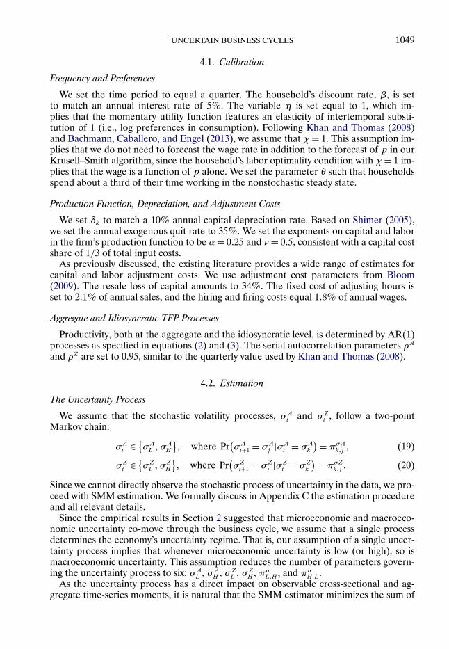
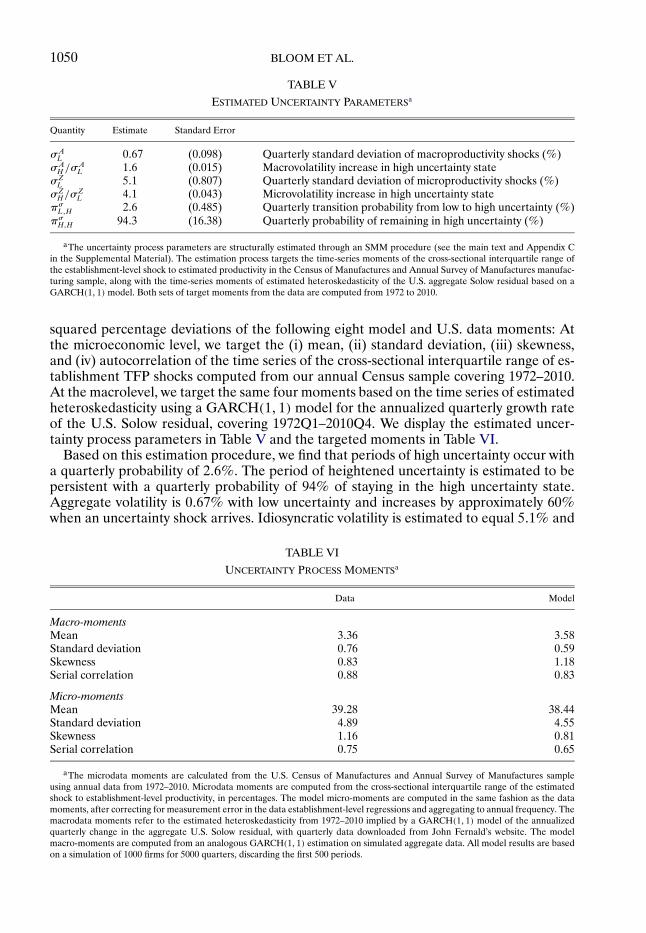
squared percentage deviations of the following eight model and U.S. data moments: Atthe microeconomic level, we target the (i) mean, (ii) standard deviation, (iii) skewness,and (iv) autocorrelation of the time series of the cross-sectional interquartile range of es-tablishment TFP shocks computed from our annual Census sample covering 1972–2010.At the macrolevel, we target the same four moments based on the time series of estimatedheteroskedasticity using a GARCH(1�1) model for the annualized quarterly growth rateof the U.S. Solow residual, covering 1972Q1–2010Q4. We display the estimated uncer-tainty process parameters in Table V and the targeted moments in Table VI.

Based on this estimation procedure, we find that periods of high uncertainty occur witha quarterly probability of 2�6%. The period of heightened uncertainty is estimated to bepersistent with a quarterly probability of 94% of staying in the high uncertainty state.Aggregate volatility is 0�67% with low uncertainty and increases by approximately 60%when an uncertainty shock arrives. Idiosyncratic volatility is estimated to equal 5�1% and

TABLE VI

UNCERTAINTY PROCESS MOMENTSa

Data Model

Macro-momentsMean 3�36 3�58Standard deviation 0�76 0�59Skewness 0�83 1�18Serial correlation 0�88 0�83

Micro-momentsMean 39�28 38�44Standard deviation 4�89 4�55Skewness 1�16 0�81Serial correlation 0�75 0�65

aThe microdata moments are calculated from the U.S. Census of Manufactures and Annual Survey of Manufactures sampleusing annual data from 1972–2010. Microdata moments are computed from the cross-sectional interquartile range of the estimatedshock to establishment-level productivity, in percentages. The model micro-moments are computed in the same fashion as the datamoments, after correcting for measurement error in the data establishment-level regressions and aggregating to annual frequency. Themacrodata moments refer to the estimated heteroskedasticity from 1972–2010 implied by a GARCH(1�1) model of the annualizedquarterly change in the aggregate U.S. Solow residual, with quarterly data downloaded from John Fernald’s website. The modelmacro-moments are computed from an analogous GARCH(1�1) estimation on simulated aggregate data. All model results are basedon a simulation of 1000 firms for 5000 quarters, discarding the first 500 periods.


it increases by approximately 310% in the heightened uncertainty state. Table V reportsthe point estimates and standard errors from the SMM estimation procedure. As thetable shows, most of these parameters are estimated precisely. However, in Section 5.2.3,we discuss the robustness of our numerical results to modification of each of these sixparameters.

It is useful at this point to explain the large estimated increase in underlying fundamen-tal microeconomic uncertainty σZt on the impact of an uncertainty shock in light of theapparently more muted fluctuations of our microeconomic uncertainty proxy in Figure 3.Although closely related and informative for one another, the two series are distinct. Cru-cially, as we discuss in detail in our estimation Appendix C, the process of constructing ourcross-sectional data proxy for microeconomic uncertainty involves time aggregation fromquarterly to annual frequency, an unavoidable temporal mismatch of the measurementof inputs and outputs within the year, as well as measurement error of productivity in theunderlying Census of Manufactures sample. In Appendix C, we demonstrate within themodel that each of these measurement steps leads to a reduction in the variability of theuncertainty proxy relative to its mean level, with the temporal mismatch between inputand output measurement, as well as measurement error itself, accounting for the bulk ofthe shift. The large increase in microeconomic uncertainty σZt , which we estimate uponimpact of an uncertainty shock, is critical for matching the behavior of measured produc-tivity shock dispersion in the data. As Table VI demonstrates, the estimated model quiteclosely captures the overall time-series properties of measured uncertainty in our data.

5. QUANTITATIVE ANALYSIS

In what follows, we explore the quantitative implications of our model. We begin bydiscussing the unconditional second moments generated by the model. We then continueby specifically studying the effects of an uncertainty shock.

5.1. Business Cycle Statistics

Table VII illustrates that the model generates second-moment statistics that resembletheir empirical counterparts in U.S. data. We simulate the model over 5000 quarters us-ing the histogram or nonstochastic simulation approach following Young (2010). We thencompute the standard set of business cycle statistics, after discarding an initial 500 quar-ters. As in the data, investment and hours co-move with output. Output and consumptionco-move, although not as much as in the data. Investment is more volatile than output,while consumption is less volatile. Given the high assumed Frisch elasticity of labor sup-ply, the model also generates a realistic volatility of hours relative to output. See Rogerson(1988), Hansen (1985), or Benhabib, Rogerson, and Wright (1991) for a discussion of un-derlying mechanisms that can generate more elastic labor supply in this class of models.Overall, we conclude that the business cycle implications of our model are consistent withthe common findings in the literature.

5.2. The Effects of an Uncertainty Shock

As has been known since at least Scarf (1959), nonconvex adjustment costs lead to Ssinvestment and hiring policy rules. Firms do not hire and invest until productivity reachesan upper threshold (the S in Ss), and do not fire and disinvest until productivity hits alower threshold (the s in Ss). This is shown for labor in Figure 5, which plots the distribu-tion of firms by their productivity/labor ratios, Az

n−1, after the micro- and macro-shocks have

1052 BLOOM ET AL.

TABLE VII

BUSINESS CYCLE STATISTICSa

Data Model

σ(x) σ(x)

σ(x) σ(y) ρ(x� y) σ(x) σ(y) ρ(x� y)

Output 1.6 1.0 1.0 2�0 1.0 1.0Investment 7.0 4.5 0.9 11�9 6.0 0.9Consumption 1.3 0.8 0.9 0�9 0.4 0.5Hours 2.0 1.3 0.9 2�4 1.2 0.8

aThe first panel contains business cycle statistics for quarterly U.S. data covering 1972Q1–2010Q4. The term σ(x) is the standarddeviation of the log variable, σ(y) is the standard deviation in log variable relative to the standard deviation of log output, and ρ(x� y)is the correlation of the log variable and log output. All business cycle data are current as of July 14, 2014. Output is real gross domesticproduct (FRED GDPC1), investment is real gross private domestic investment (GPDIC1), consumption is real personal consumptionexpenditures (PCECC96), and hours is total nonfarm business sector hours (HOANBS). The second panel contains business cyclestatistics from unconditional simulation of the estimated model, computed from a 5000-quarter simulation with the first 500 periodsdiscarded. All series are HP-filtered with smoothing parameter 1600, in logs expressed as percentages.

been drawn but before firms have adjusted. On the right is the firm-level hiring threshold(right solid line) and on the left the firing threshold (left solid line), in the case of lowuncertainty. Firms to the right of the hiring line will hire, firms to the left of the firing linewill fire, and those in the middle will be inactive for the period.

An increase in uncertainty increases the returns to inaction, shown by the increasedhiring threshold (right dotted line) and reduced firing threshold (left dotted line). Whenuncertainty is high, firms become more cautious as labor adjustment costs make it expen-

FIGURE 5.—The impact of an increase in uncertainty on the hiring and firing thresholds. Notes: The figureplots the simulated cross-sectional marginal distribution of micro-level labor inputs after productivity shockrealizations and before labor adjustment. The distribution plots a representative period with average aggregateproductivity and low uncertainty levels. The vertical hiring and firing thresholds are computed based on firmpolicy functions with average micro-level productivity realizations, taking as given the aggregate state of theeconomy with low uncertainty (solid lines) and a high uncertainty counterfactual (dotted lines).


sive to make a hiring or firing mistake. Hence, the hiring and firing thresholds move out,increasing the range of inaction. This leads to a fall in net hiring, since the mass of firmsis right-shifted due to labor attrition. A similar phenomenon occurs with capital, wherebyincreases in uncertainty reduce the amount of net investment.

5.2.1. Modelling a Pure Uncertainty Shock

To analyze the aggregate impact of uncertainty, we independently simulate 2500economies, each of 100-quarter length. The first 50 periods are simulated unconditionally,so all exogenous processes evolve normally. Then for each economy, after 50 quarters, weinsert an uncertainty shock by imposing a high uncertainty state. From the shock periodonward each economy evolves normally. To calculate the impulse response function to anuncertainty shock for any macrovariable, we first compute the average of the aggregatevariable in each period t across simulated economies. The effect of an uncertainty shockis then simply given by the percentage deviation of the average in period t from its valuein the pre-shock period.

Figure 6 depicts the impact of an uncertainty shock on output. For graphical purposes,period 0 in the figure corresponds to the pre-shock period in the above discussion, that is,quarter 50. Figure 6 displays a drop in output of just over 2.5% within one quarter. Thissignificant fall is one of the key results of this paper as it shows that uncertainty shocks canbe a quantitatively important contributor to business cycles within a general equilibriumframework. A quick recovery follows the initial decline, and output returns to normallevels within 1 year. We note that output then declines again moderately from quarters 6onward. We defer the discussion for the intuition behind this result until Section 5.2.4.

These dynamics in output arise from the dynamics in three channels: labor, capital,and the misallocation of factors of production. These are depicted in Figure 7. First, in

FIGURE 6.—The effects of an uncertainty shock. Notes: Based on independent simulations of 2500economies of 100-quarter length. We impose an uncertainty shock in the quarter labelled 1, allowing normalevolution of the economy afterwards. We plot the percent deviation of cross-economy average output from itsvalue in quarter 0.

1054 BLOOM ET AL.

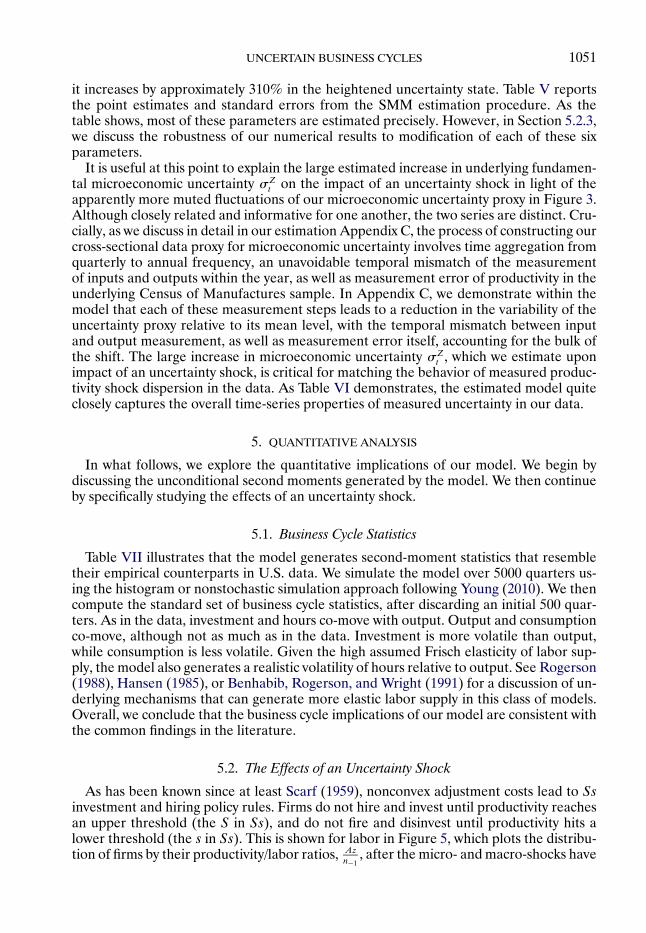
FIGURE 7.—Labor and investment drop and rebound, misallocation rises, and consumption overshootsthen falls. Notes: Based on independent simulations of 2500 economies of 100-quarter length. We impose anuncertainty shock in the quarter labelled 1, allowing normal evolution of the economy afterwards. Clockwisefrom the top left, we plot the percent deviations of cross-economy average labor, investment, consumption,and the dispersion of the marginal product of labor from their values in quarter 0.

the top-left panel, we plot the time path of hours worked. When uncertainty increases,most firms pause hiring, and hours worked begin to drop because workers are continuingto attrit from firms without being replaced. In the model, this rate of exogenous attri-tion is assumed to be constant over the cycle. This is consistent with Shimer (2005) andHall (2005), who show that around three-quarters of the movements in the volatility ofunemployment are due to job-finding rates and not to the cyclicality of the destructionrate. Similarly, in the top-right panel, we plot the time path of investment, which dropsrapidly due to the increase in uncertainty. Since investment falls but capital continues todepreciate, there is also a drop in the capital stock.

Misallocation of factor inputs—using the terminology of Hsieh and Klenow (2009)—increases in the economy in response to an uncertainty shock. In normal times, unpro-ductive firms contract and productive firms expand, helping to maintain high levels ofaggregate productivity. But when uncertainty is high, firms reduce expansion and con-traction, shutting off much of this productivity-enhancing reallocation. In the bottom-leftpanel, we plot the path of the dispersion of the marginal product of labor after an un-certainty shock. More precisely, the bottom-left panel plots the impulse response of thecross-sectional standard deviation of log( y

n). In the wake of an uncertainty shock, labor

misallocation endogenously worsens, improving only slowly. In the longer run, labor, in-vestment, misallocation, and output all start to recover to their steady state, as the uncer-tainty shock is temporary. As uncertainty falls back, firms start to hire and invest againto address their pent-up demand for labor and capital. In Figure B3 in the Supplemen-tal Material, we depict alternative measures of misallocation. As Figure B3 shows, all ofthese alternative measures point to the same result of increased misallocation followingan uncertainty shock.

In the lower-right panel of Figure 7, we plot the time profile of consumption. When theuncertainty shock occurs, consumption jumps up in the first quarter before subsequently


falling back below the mean of the ergodic distribution for several quarters. The logicbehind this initial increase in consumption is as follows. In the impact period of the un-certainty shock, that is, period 1 in Figure 7, the households understand that the degreeof misallocation has increased in the economy as the bottom-left panel demonstrates. In-creased misallocation acts as a negative first-moment shock to aggregate productivity andthus lower the expected return on savings, making immediate consumption more attrac-tive and thus leading to its first-period increase. Furthermore, this jump in consumptionis feasible since, in the impact period of the uncertainty shock, the freeze in both invest-ment and hiring reduces the resources spent on capital and adjustment costs, thus freeingup resources. After this initial jump, starting in period 2 in Figure 7, the capital stock isnow below its ergodic distribution, where we note that in the impact period of the un-certainty shock, the pre-shock aggregate capital level was fixed. This fact, together withhours worked being below their ergodic distribution and the degree of misallocation beingabove its ergodic distribution, limits the overall resources in the economy and thus limitsconsumption. In addition, the economy begins its recovery in period 2 in Figure 7, whichis manifested in investment and hiring beginning to increase relative to the values exhib-ited during the impact period of the uncertainty shock. This recovery requires resourcesto be spent on capital and adjustment costs, further reducing the available resources forconsumption. Interestingly, we note that Khan and Thomas (2013) find in their modelof credit constraints that while output, labor, and investment fall in response to a credittightening shock, in fact consumption, as in our model, also initially rises due to similargeneral equilibrium effects.

Clearly, this rise in consumption at the start of recessions is an unattractive feature ofa pure uncertainty shock model of business cycles. Several options exist, however, to tryand address this. One is to allow consumers to save in other technologies besides capi-tal, for example, in foreign assets. This is the approach Fernandez-Villaverde et al. (2011)take in modelling risk shocks in small open economies. In an open economy model, a do-mestic uncertainty shock induces agents to increase their savings abroad (capital flight).In our closed model this is not possible, but extending the model to allow a foreign sec-tor would make this feasible, although computationally more intensive. Another optionwould be to use utility functions such as those in Greenwood, Hercowitz, and Huffman(1988). Due to the complementarity between consumption and hours in such preferencestructures, they should reduce the overshoot in consumption. We do not explore theseoptions for the following two reasons. Having another investment vehicle such as foreignbond would add an additional state variable to the problem, and switching the prefer-ence structure would require us to forecast wages separately from marginal utility. Bothchanges would increase the computational burden considerably. Another option would beto model precautionary behavior from households in the wake of an uncertainty shock, asBasu and Bundick (2016) do in a new-Keynesian environment with demand-determinedoutput. Such behavior would allow for natural investment, consumption, and output co-movement, but expanding the aggregate structure of the model to account for nominalrigidities is beyond the scope of the current paper.

5.2.2. First-Moment and Second-Moment Shocks

Our quantitative results so far reveal that uncertainty shocks can contribute importantlyto recessions, but there are at least two unattractive implications of modelling an uncer-tainty shock in isolation. First, the empirical evidence in Section 2 suggests that recessionsare periods of both first- and second-moment shocks, at least to the extent that the aver-age growth rates of TFP and output decrease and their variances increase. Second, in our

1056 BLOOM ET AL.

FIGURE 8.—Adding a −2% first-moment shock increases the output fall and eliminates a consumptionovershoot. Notes: Based on independent simulations of 2500 economies of 100-quarter length. For the base-line (× symbols) we impose an uncertainty shock in the quarter labelled 1. For the uncertainty and TFP shock(� symbols), we also impose an aggregate productivity shock with average equal to −2%, allowing normal evo-lution of the economy afterwards. Clockwise from the top left, we plot the percent deviations of cross-economyaverage output, labor, consumption, and investment from their values in quarter 0.

model, uncertainty shocks are associated with an increase in consumption on impact anda reduction in disinvestment and firing (see Figures 5 and 7).

Thus, to generate an empirically more realistic simulation, we consider the combinationof an uncertainty shock and a −2% exogenous first-moment shock. See Appendix B for adiscussion of the specific numerical experiment considered here.

As Figure 8 suggests, this additional shock magnifies the drop in output, investment,and hours. The addition of the first-moment shock also leads to a fall in consumption onimpact. Given the business cycle co-movement we observe empirically, we conclude thatsimultaneous first- and second-moment shocks in the model can generate dynamics thatresemble recent U.S. recessions.

5.2.3. Robustness

In this section, we discuss the robustness of our finding to different parameterizations.We first consider the robustness of our results with respect to the estimated parametersgoverning the uncertainty process. Since the estimated values in Section 4.2 pointed to(i) a significant jump in both micro- and macro-uncertainty, (ii) a significant persistenceof the uncertainty process, and (iii) a moderately high frequency of high uncertainty,we consider experiments where we reduce the values of each of these parameters. Forconsistency, unless otherwise noted, every robustness experiment considers a reductionof 25% in the parameter value. Thus, within this set we consider (i) a reduction of themacrovolatility jump, σ

AH

σAL, from 1�6 to 1�2, (ii) a reduction of the microvolatility jump, σ

zH

σzL,

from 4�13 to 3�10, (iii) a reduction in the likelihood of transition from low uncertainty tohigh uncertainty, πσL�H , from 0�026 to 0�02, and (iv) a reduction in the uncertainty per-sistence, πσH�H , from 0�94 to 0�71. Finally, we also consider two additional experiments


FIGURE 9.—The impact of an uncertainty shock is robust to a wide range of alternative calibrations. Notes:Based on independent simulations of 2500 economies of 100-quarter length. For all simulations we impose anuncertainty shock in the quarter labelled 1, allowing normal evolution of the economy afterwards. Baseline(× symbols) is the estimated baseline path. Other paths plot responses assuming a reduction in low-uncer-tainty micro volatility (σZ

L , ◦ symbols), the high-uncertainty increase in micro volatility (σZH/σ

ZL , � symbols),

low-uncertainty macro volatility (σAL , + symbols), the high-uncertainty increase in macro volatility (σA

H/σAL , ∗

symbols), the frequency of an uncertainty shock (πσL�H , stars), the persistence of an uncertainty shock (πσH�H ,� symbols), all adjustment costs for labor and capital (� symbols). Clockwise from the top left, we plot thepercent deviations of cross-economy average output, labor, consumption, and investment from their values inquarter 0.

where (i) we lower the microvolatility baseline value, σzL, from 0�051 to 0�038 and (ii) welower macrovolatility baseline value, σAL , from 0�0067 to 0�0050. Figure 9 plots the effectsof each of these variations on output, investment, labor, and consumption. As Figure 9suggests, the results are overall robust to these changes, preserving the dynamics reportedin Figures 6–8. The one exception is the reduction in the persistence of the uncertaintyshock to 0.7 from the estimated value of 0.94. At lower levels of persistence, the impact isshort-lived. This highlights how the dynamics of the impact of uncertainty shocks are sen-sitive to the persistence of the underlying shock and is another motivation for our SMMestimation of the parameters of the uncertainty process. We note that the estimated valueof 0.94 for the autocorrelation of uncertainty may seem high. However, this potentiallyaccounts for the endogenous amplification of uncertainty from slower growth proposedby a range of other papers.

In addition to systematically plotting robustness checks to changes in the value of eachof our six estimated uncertainty process parameters, Figure 9 also plots the results fromone additional experiment in which we reduce the value of all capital and labor adjust-ment cost parameters by 25% simultaneously. The effect of an uncertainty shock changeslittle relative to our baseline, a result that reflects the fact, well known within the liter-ature on investment and adjustment costs, that the sizes of inaction regions are concavefunctions of adjustment costs. For example, see the analytical results in Dixit (1995) andAbel and Eberly (1996) that show that the size of the inaction region for investment intheir models expands to the third or fourth order in adjustment costs around zero.

1058 BLOOM ET AL.

FIGURE 10.—The impact of an uncertainty shock combines Oi–Hartman–Abel, real options and consump-tion smoothing effects. Notes: Based on independent simulations of 2500 economies of 100-quarter length.For all simulations we impose an uncertainty shock in the quarter labelled 1, allowing normal evolution of theeconomy afterwards. GE, adjustment costs (× symbols) is the baseline, and the PE responses are partial equi-librium paths with adjustment costs (+ symbols) and without adjustment costs (◦ symbols). Clockwise fromthe top left, we plot the percent deviations of cross-economy average output, labor, consumption, and invest-ment from their values in quarter 0. Note that PE economies have no consumption concept, with deviationstherefore set to 0.

5.2.4. Decomposing the Impact of Uncertainty

The next set of robustness results studies how the effects of uncertainty shocks differacross general equilibrium (GE) and partial equilibrium (PE) frameworks. To addressthis question, we plot in Figure 10 the impact of an uncertainty shock in three differenteconomies. The line with × symbols depicts again the effects of an uncertainty shockin our GE model economy, the line with + symbols depicts the same response but withPE only (all prices and wages are held constant and the consumer side of the economyis ignored), while the line with ◦ symbols depicts the effects of an uncertainty shock ina PE economy with no adjustment costs at all. Note that in the bottom-right panel inthe PE economies, consumption is not defined because there is no notion of an aggre-gate household. We therefore impose a zero response path for consumption in thosecases.

When there are no adjustment costs of any type in a PE economy, output actually in-creases following an uncertainty shock. The reason for this result is related to the Oi(1961), Hartman (1972), and Abel (1983) effect, whereby a higher variance of productiv-ity increases investment, hiring, and output because the optimal capital and labor choicesare convex in productivity.

By contrast, the addition of adjustment costs to the PE setup dramatically changes theeffect of an uncertainty shock. Now, on impact there is a fall in aggregate output. Thereason is that the increase in uncertainty moves firms’ labor and capital Ss bands out,temporarily pausing hiring and investment. If all firms pause hiring and investment, ag-gregate labor and capital drop due to labor attrition and capital depreciation. But thispause is short-lived, as once uncertainty drops back, firms start to hire and invest again.


So in the medium run, the Oi–Hartman–Abel effect dominates and output rises above itslong-run trend.

While these forces are also present in the baseline GE adjustment cost economy, thecurvature in the utility function, that is, the endogenous movement in the interest rate,moderates the rebound and overshoot. The overshoot in the PE economy requires bigmovements in investment and labor, which are feasible since consumption is not takeninto account in the PE framework. However, in the GE framework, the curvature in utilityslows down the rebound of the GE economy, generating a smoother and more persistentoutput cycle. Intriguingly, in the first period, however, GE has very little impact on outputrelative to the PE economy with adjustment cost. This is because the Ss bands have movedso far out that there is a reduced density of firms near the hiring or investment thresholdsto respond to prices. Hence, the short-run robustness of the impact of uncertainty shocksto GE suggested by Bloom (2009) seems to be present, while the medium-run sensitivityto GE highlighted by Thomas (2002) and Khan and Thomas (2003, 2008) is also present.

We are now in position to discuss the reason for the sluggish behavior of output inthe medium term after an uncertainty shock in Figure 6. First, on impact in periods 1and 2, the “real options” effect due to the uncertainty shock dominates, leading to ahiring/investment freeze, misallocation, and, thus, a significant drop in output. Later onin periods 3–5, the economy exhibits a “rebound” as the high microvolatility is realizedand some firms draw significantly higher productivity shocks than before. Firms start toreadjust and the Oi–Hartman–Abel effect leads to a recovery. During the third stagestarting in periods 6–8, output declines again.

Two factors play a role in the second fall in output. First, the level of misallocationremains high, which acts as a drag on output and is a large contributor to the slowdown ofthe recovery. The bottom-left panel of Figure 7 reveals that the cross-sectional dispersionof the marginal product of labor—a measure of labor misallocation—remains almost 10%higher in period 6 and declines only slowly as firms begin to adjust their inputs again in thewake of an uncertainty shock. Underlying misalignment of inputs and productivity at themicrolevel prevents effective use of the capital and labor stock of the aggregate economy,and meaningful input adjustment costs prevent such misallocation from resolving itselfquickly over this period.

The second factor contributing to the second more gradual decline in output is a de-clining path for investment starting around period 6. By this stage, the real options effecthas subsided in large part and the economy has a low but growing consumption path.This results in a declining path of interest rates over which it is optimal to have a de-clining investment path. These investment dynamics of the economy in the third stage ofthe response to an uncertainty shock resemble those that show up in a basic neoclassicalgrowth model as in Brock and Mirman (1972). Figure D1 in the Supplemental Materialplots the response of such an economy to a capital destruction shock. As the figure shows,consumption converges from below at a declining rate, and investment declines over thepath.

5.2.5. Laws of Motion Robustness

Our final set of robustness checks studies the impact of variations in the labor andcapital depreciation rates. In these experiments we vary one by one the capital deprecia-tion rate and the labor depreciation rate by one quarter each. The results are depicted inFigure 11. As the figure suggests, unsurprisingly reduction of the labor depreciation rateattenuates the fall in hours and thus in output but preserves the overall dynamics found inthe benchmark calibration. Changes in the capital depreciation rate do not change the fall

1060 BLOOM ET AL.

FIGURE 11.—The impact of an uncertainty shock is reduced by lower rates of capital depreciation or laborattrition. Notes: Based on independent simulations of 2500 economies of 100-quarter length. For all simu-lations we impose an uncertainty shock in the quarter labelled 1, allowing normal evolution of the economyafterwards. Baseline (× symbols) is the estimated baseline path. The two other paths plot responses assuminga 25% reduction in the capital depreciation rate (◦ symbols) and labor depreciation rate (+ symbols). Clock-wise from the top left, we plot the percent deviations of cross-economy average output, labor, consumption,and investment from their values in quarter 0.

on impact, which is driven by the behavior in labor. Later on, a lower capital depreciationrate accentuates the recovery from an uncertainty shock as it induces a strong reboundin investment leading to an increase in capital and thus in labor and output. However,we note that the more empirically relevant exercise is to increase the capital depreciationrate, since investment is increasingly shifting toward intangible areas, which have muchhigher depreciation rates. For example, the Bureau of Economic Analysis’s (BEA) migra-tion of R&D from the satellite accounts to the fixed assets tables is based on depreciationrates of around 20% or higher (Li (2012)). Thus, while the reduction in annual deprecia-tion does reduce the impact of an uncertainty shock, the empirically relevant depreciationrate in the economy is likely much higher.

6. POLICY IN THE PRESENCE OF UNCERTAINTY

In this section, we analyze the effects of stimulative policies in the presence of uncer-tainty shocks. It is important to emphasize that any such policy is not optimal within thecontext of our model, as the competitive equilibrium is Pareto optimal. Rather, we seeour policy experiments as a means to document and quantify the effects of such policiesin times of heightened uncertainty. It is also worth noting that this ignores the direct im-pact of policy on uncertainty as studied by papers such as Baker, Bloom, and Davis (2016)and Hassan, Hollander, van Lent, and Tahoun (2017).

The policy experiment we consider is a policy that attempts to temporarily stimulatehiring by reducing the effective wage paid by firms. More specifically, the policy consistsof an unanticipated 1% wage bill subsidy paid for one quarter and financed through alump-sum tax on households. We simulate this policy impulse once during an uncertaintyshock and also in an economy that is not hit by an uncertainty shock. By comparing the


FIGURE 12.—Policy is less effective in the aftermath of an uncertainty shock. Notes: Based on independentsimulations of 2500 economies of 100-quarter length. For a wage subsidy in normal times (black bar, left),we provide an unanticipated 1% wage bill subsidy to all firms in quarter 1, allowing the economy to evolvenormally thereafter. We also simulate an economy with no wage subsidy in quarter 1. The bar height is thepercentage difference between the cross-economy average subsidy and no subsidy output paths in quarter 1.For the wage subsidy with an uncertainty shock (red bar, right), we repeat the experiment but simultaneouslyimpose an uncertainty shock in quarter 1.

marginal effect in those two cases, we attempt to identify the effect of uncertainty onpolicy effectiveness.

Figure 12 depicts this experiment as it shows the net impact of the policy. That is, wefirst solve for the effects of the policy on output when it does not coincide with an uncer-tainty shock. Subtracting from this the behavior of output when there is no uncertaintyshock and no subsidy yields the net impact of the policy in the absence of an uncertaintyshock. We then solve for the policy’s effect when it does coincide with an uncertaintyshock. Similarly, subtracting from this latter experiment the behavior of output whenthere is an uncertainty shock and no subsidy, the behavior depicted in Figure 6 yieldsthe net impact of the policy in the presence of an uncertainty shock. As Figure 12 shows,the presence of uncertainty reduces the effects of the wage policy by over two-thirds onimpact. The reason is that as soon as uncertainty rises, the Ss thresholds jump out, somany firms are far away from their hiring and investment thresholds, making them lessresponsive to any policy stimulus. Our results here echo findings from the lumpy invest-ment literature on the procyclicality of the investment response to productivity shocks(e.g., Bachmann, Caballero, and Engel (2013)). In particular, we show that uncertaintyor second-moment shocks in addition to first-moment shocks can also generate move-ment in the responsiveness of the economy to shocks. Interestingly, in the context of anew-Keynesian economy with a distinct structure and policy experiment, Vavra (2014)also finds that second-moment shocks reduce the responsiveness of the economy to pol-icy.

Overall, our results highlight how uncertainty shocks lead to time-varying policy ef-fectiveness. At the instant an uncertainty shock hits, policy is not as effective relative tonormal times. Hence, uncertainty shocks not only impact the economy directly, but alsoindirectly change the response of the economy to any potential reactive stabilization pol-icy.

1062 BLOOM ET AL.

7. CONCLUSIONS

Uncertainty has received substantial attention as a potential factor in business cycles.The first part of this paper uses Census microdata to show that measured uncertainty isindeed strongly countercyclical. This is true both at the aggregate and the industry level:slower industry growth is associated with higher industry uncertainty.

The second part of the paper then builds a DSGE model with heterogeneous firms,time-varying uncertainty, and adjustment costs to quantify the impact of second-momentshocks. We find that uncertainty shocks typically lead to drops of about 2.5% in GDP,with a sharp drop, quick recovery, and then continued sluggishness in output. This sug-gests that uncertainty could play an important role in driving business cycles, either as animpulse or amplification mechanism. We also find that because uncertainty makes firmscautious, the response of the economy to stimulative policy substantially declines. Finally,both our empirical and simulation results suggest recessions are best modelled as a com-bination of a negative first-moment and a positive second-moment shock.

REFERENCES

ABEL, A. (1983): “Optimal Investment Under Uncertainty,” American Economic Review, 73, 228–233. [1058]ABEL, A. B., AND J. C. EBERLY (1996): “Optimal Investment With Costly Reversibility,” Review of Economic

Studies, 63 (4), 581–593. [1034,1057]ARELLANO, C., Y. BAI, AND P. KEHOE (2012): “Financial Markets and Fluctuations in Uncertainty,” Working

Paper, Federal Reserve Bank of Minneapolis. [1034]BACHMANN, R., AND R. BAYER (2013): ““Wait-and-See” Business Cycles?” Journal of Monetary Economics,

60 (6), 704–719. [1034](2014): “Investment Dispersion and the Business Cycle,” American Economic Review, 104 (4), 1392–

1416. [1034,1036]BACHMANN, R., AND G. MOSCARINI (2011): “Business Cycles and Endogenous Uncertainty,” Report,

Yale. [1041]BACHMANN, R., R. J. CABALLERO, AND E. M. R. A. ENGEL (2013): “Aggregate Implications of Lumpy In-

vestment: New Evidence and a DSGE Model,” American Economic Journal: Macroeconomics, 5 (4), 29–67.[1034,1046,1049,1061]

BAKER, S., N. BLOOM, AND S. DAVIS (2016): “Measuring Economic Policy Uncertainty,” Quarterly Journal ofEconomics, 131 (4), 1593–1636. [1060]

BASU, S., AND B. BUNDICK (2017): “Uncertainty Shocks in a Model of Effective Demand,” Econometrica, 85(3), 937–958. [1034,1055]

BASU, S., J. FERNALD, AND M. S. KIMBALL (2006): “Are Technology Improvements Contractionary?” Ameri-can Economic Review, 96 (5), 1418–1448. [1042]

BEKAERT, G., R. J. HODRICK, AND X. ZHANG (2012): “Aggregate Idiosyncratic Volatility,” Journal of Financialand Quantitative Analysis, 47 (6), 1155–1185. [1038]

BENHABIB, J., R. ROGERSON, AND R. WRIGHT (1991): “Homework in Macroeconomics: Household Produc-tion and Aggregate Fluctuations,” Journal of Political Economy, 99 (6), 1166–1187. [1051]

BERGER, D., AND J. VAVRA (2015): “Volatility and Pass-Through,” Working Paper. [1036]BERNANKE, B. (1983): “Irreversibility, Uncertainty and Cyclical Investment,” Quarterly Journal of Economics,

98, 85–106. [1034,1036]BERTOLA, G., AND R. J. CABALLERO (1994): “Irreversibility and Aggregate Investment,” Review of Economic

Studies, 61, 223–246. [1034]BLOOM, N. (2009): “The Impact of Uncertainty Shocks,” Econometrica, 77, 623–685. [1034,1044,1048,1049,

1059](2014): “Fluctuations in Uncertainty,” Journal of Economic Perspectives, 28 (2), 153–176. [1042]

BLOOM, N., S. BOND, AND J. VAN REENEN (2007): “Uncertainty and Investment Dynamics,” Review of Eco-nomic Studies, April, 74, 391–415. [1042]

BLOOM, N., M. FLOETOTTO, N. JAIMOVICH, I. SAPORTA-EKSTEN, AND S. J. TERRY (2018): “Supplementto ‘Really Uncertain Business Cycles’,” Econometrica Supplemental Material, 86, https://doi.org/10.3982/ECTA10927. [1034,1047]

BROCK, W., AND L. MIRMAN (1972): “Optimal Economic Growth and Uncertainty: The Discounted Case,”Journal of Economic Theory, 4 (3), 479–513. [1059]

http://www.e-publications.org/srv/ecta/linkserver/setprefs?rfe_id=urn:sici%2F0012-9682%28201805%2986%3A3%3C1031%3ARUBC%3E2.0.CO%3B2-6

http://www.e-publications.org/srv/ecta/linkserver/openurl?rft_dat=bib:1/1&rfe_id=urn:sici%2F0012-9682%28201805%2986%3A3%3C1031%3ARUBC%3E2.0.CO%3B2-6


































CABALLERO, R. J., AND E. M. R. A. ENGEL (1993): “Microeconomic Adjustment Hazards and AggregateDynamics,” Quarterly Journal of economics, 108, 359–383. [1044]

(1999): “Explaining Investment Dynamics in U.S. Manufacturing: A Generalized Ss Approach,”Econometrica, 67 (4), 783–826. [1034,1044]

CAMPBELL, J., M. LETTAU, B. MALKIEL, AND Y. XU (2001): “Have Individual Stocks Become More Volatile?An Empirical Exploration of Idiosyncratic Risk,” Journal of Finance, 56 (1), 1–43. [1038,1042]

CHAMLEY, C., AND D. GALE (1994): “Information Revelation and Strategic Delay in a Model of Investment,”Econometrica, 62 (5), 1065–1085. [1041]

CHRISTIANO, L. J., R. MOTTO, AND M. ROSTAGNO (2014): “Risk Shocks,” American Economic Review, 104(1), 27–65. [1034]

COOPER, R., J. HALTIWANGER, AND J. L. WILLIS (2015): “Dynamics of Labor Demand: Evidence From Plant-Level Observations and Aggregate Implications,” Research in Economics, 69, 37–50. [1044]

COOPER, R. W., AND J. C. HALTIWANGER (2006): “On the Nature of Capital Adjustment Costs,” Review ofEconomic Studies, 73, 611–633. [1044]

DIXIT, A. (1995): “Irreversible Investment With Uncertainty and Scale Economies,” Journal of Economic Dy-namics and Control, 19 (1–2), 327–350. [1057]

DIXIT, A. K., AND R. S. PINDYCK (1994): Investment Under Uncertainty. Princeton: Princeton UniversityPress. [1034]

ENGLE, R. F., AND J. G. RANGEL (2008): “The Spline-GARCH Model for Low-Frequency Volatility and ItsGlobal Macroeconomic Causes,” Review of Financial Studies, 21 (3), 1187–1222. [1042]

FAJGELBAUM, P. D., E. SCHAAL, AND M. TASCHEREAU-DUMOUCHEL (2017): “Uncertainty Traps,” QuarterlyJournal of Economics, 132 (4), 1641–1692. [1041]

FERNANDEZ-VILLAVERDE, J., P. GUERRÓN-QUINTANA, J. RUBIO-RAMIREZ, AND M. URIBE (2011): “RiskMatters: The Real Effects of Volatility Shocks,” The American Economic Review, 101 (6), 2530–2561. [1034,

1055]FERNANDEZ-VILLAVERDE, J., P. A. GUERRÓN-QUINTANA, K. KUESTER, AND J. RUBIO-RAMIREZ (2015): “Fis-

cal Volatility Shocks and Economic Activity,” American Economic Review, 105 (11), 3352–3384. [1034]FOSTER, L., J. HALTIWANGER, AND C. J. KRIZAN (2000): “Aggregate Productivity Growth: Lessons From

Microeconomic Evidence,” in New Developments in Productivity Analysis. NBER, University of ChicagoPress. [1033,1035]

(2006): “Market Selection, Reallocation and Restructuring in the U.S. Retail: Trade Sector in the1990s,” Review of Economics and Statistics, 88, 748–758. [1033]

FOSTER, L., J. HALTIWANGER, AND C. SYVERSON (2008): “Reallocation, Firm Turnover, and Efficiency: Se-lection on Productivity or Profitability?” American Economic Review, 98 (1), 394–425. [1035]

GILCHRIST, S., J. SIM, AND E. ZAKRAJŠEK (2014): “Uncertainty, Financial Frictions, and Investment,” WorkingPaper 20038, NBER. [1034]

GOURIO, F., AND A. K. KASHYAP (2007): “Investment Spikes: New Facts and a General Equilibrium Explo-ration,” Journal of Monetary Economics, 54, 1–22. [1034]

GREENWOOD, J., Z. HERCOWITZ, AND G. W. HUFFMAN (1988): “Investment, Capacity Utilization, and theReal Business Cycle,” American Economic Review, 78 (3), 402–417. [1055]

GUVENEN, F., S. OZKAN, AND J. SONG (2014): “The Nature of Countercyclical Income Risk,” Journal of Polit-ical Economy, 122 (3), 621–660. [1036]

HALL, R. E. (2004): “Measuring Factor Adjustment Costs,” Quarterly Journal of Economics, 119 (3), 899–927.[1044]

(2005): “Job Loss, Job Finding, and Unemployment in the U.S. Economy Over the Past Fifty Years,”NBER Macroeconomics Annual, 101–137. [1054]

HANSEN, G. D. (1985): “Indivisible Labor and the Business Cycle,” Journal of Monetary Economics, 16 (3),309–327. [1051]

HARTMAN, R. (1972): “The Effect of Price and Cost Uncertainty on Investment,” Journal of Economic Theory,5, 258–266. [1058]

HASSAN, T. A., S. HOLLANDER, L. VAN LENT, AND A. TAHOUN (2017): “Firm-Level Political Risk: Measure-ment and Effects,” Working Paper 24029, NBER. [1060]

HASSLER, J. (1996): “Variations in Risk and Fluctuations in Demand—a Theoretical Model,” Journal of Eco-nomic Dynamics and Control, 20, 1115–1143. [1034]

HAYASHI, F. (1982): “Tobin’s Marginal q and Average q: A Neoclassical Interpretation,” Econometrica, 50 (1),213–224. [1044]

HOPENHAYN, H., AND R. ROGERSON (1993): “Job Turnover and Policy Evaluation: A General EquilibriumAnalysis,” Journal of Political Economy, 101, 915–938. [1034]












http://www.e-publications.org/srv/ecta/linkserver/openurl?rft_dat=bib:33/F14&rfe_id=urn:sici%2F0012-9682%28201805%2986%3A3%3C1031%3ARUBC%3E2.0.CO%3B2-6
























http://www.e-publications.org/srv/ecta/linkserver/openurl?rft_dat=bib:33/F14&rfe_id=urn:sici%2F0012-9682%28201805%2986%3A3%3C1031%3ARUBC%3E2.0.CO%3B2-6












1064 BLOOM ET AL.

HOUSE, C. L. (2014): “Fixed Costs and Long-Lived Investments,” Journal of Monetary Economics, 68, 86–100.[1034]

HSIEH, C.-T., AND P. J. KLENOW (2009): “Misallocation and Manufacturing TFP in China and India,” QuarterlyJournal of Economics, 124 (4), 1403–1448. [1054]

JURADO, K., S. LUDVIGSON, AND S. NG (2015): “Measuring Uncertainty,” American Economic Review, 105(3), 1177–1216. [1036,1042]

KEHRIG, M. (2015): “The Cyclical Nature of the Productivity Distribution,” Working Paper. [1034,1036]KHAN, A., AND J. K. THOMAS (2003): “Nonconvex Factor Adjustment in Equilibrium Business Cycle Models:

Do Nonlinearities Matter?” Journal on Monetary Econometrica, 50, 331–360. [1059](2008): “Idiosyncratic Shocks and the Role of Nonconvexities in Plant and Aggregate Investment

Dynamics,” Econometrica, 76 (2), 395–436. [1034,1046,1048,1049,1059](2013): “Credit Shocks and Aggregate Fluctuations in an Economy With Production Heterogeneity,”

Journal of Political Economy, 121, 1055–1107. [1034,1055]KING, R. G., AND S. T. REBELO (1999): “Resuscitating Real Business Cycles,” in Handbook of Macroeconomics,

ed. by J. B. Taylor and M. Woodford. Elsevier. [1033]KRUSELL, P., AND A. A. SMITH (1998): “Income and Wealth Heterogeneity in the Macroeconomy,” Journal of

Political Economy, 106 (5), 867–896. [1047]LEAHY, J., AND T. WHITED (1996): “The Effects of Uncertainty on Investment: Some Stylized Facts,” Journal

of Money Credit and Banking, 28, 64–83. [1042]LI, W. C. Y. (2012): “Depreciation of Business R&D Capital,” BEA staff paper. [1060]LUBOS, P., AND P. VERONESI (2013): “Political Uncertainty and Risk Premia,” Journal of Financial Economics,

110, 520–545. [1041]MERZ, M., AND E. YASHIV (2007): “Labor and the Market Value of the Firm,” American Economic Review, 97

(4), 1419–1431. [1044]NICKELL, S. J. (1986): “Dynamic Models of Labor Demand,” in Handbook of Labor Economics, ed. by

O. Ashenfelter and R. Layard. Amsterdam: North-Holland. [1044]OI, W. (1961): “The Desirability of Price Instability Under Perfect Competition,” Econometrica, 29 (1), 58–64.

[1058]ORLIK, A., AND A. VELDKAMP (2015): “Understanding Uncertainty Shocks and the Role of the Black Swan,”

NYU Report. [1041]PANOUSI, V., AND D. PAPANIKOLAOU (2012): “Investment, Idiosyncratic Risk, and Ownership,” Journal of Fi-

nance, 67 (3), 1113–1148. [1042]PETROSKY-NADEAU, N., AND E. WASMER (2013): “The Cyclical Volatility of Labor Markets Under Frictional

Financial Markets,” American Economic Journal: Macroeconomics, 5 (1), 193–221. [1041]RAMEY, V. A., AND M. D. SHAPIRO (2001): “Displaced Capital: A Study of Aerospace Plant Closings,” Journal

of Political Economy, 109, 605–622. [1044]ROGERSON, R. (1988): “Indivisible Labor, Lotteries and Equilibrium,” Journal of Monetary Economics, 21 (1),

3–16. [1051]ROMER, C. (1990): “The Great Crash and the Onset of the Great Depression,” Quarterly Journal of Economics,

105, 597–624. [1034]SCARF, H. (1959): “The Optimality of Policies in the Dynamic Inventory Problem,” in Mathematical Methods

in the Social Sciences, ed. by K. J. Arrow. Stanford University Press. [1051]SCHWERT, G. W. (1989): “Why Does Stock Market Volatility Change Over Time?” Journal of Finance, 44,

1115–1153. [1042]SHIMER, R. (2005): “The Cyclical Behavior of Equilibrium Unemployment and Vacancies,” American Eco-

nomic Review, 95 (1), 25–49. [1048,1049,1054]STOCK, J. H., AND M. W. WATSON (2012): “Disentangling the Channels of the 2007–2009 Recession,” Brook-

ings Papers on Economic Activity, Spring, 81–156. [1042]THOMAS, J. K. (2002): “Is Lumpy Investment Relevant for the Business Cycle?” Journal of Political Economy,

110 (3), 508–534. [1034,1059]VAN NIEUWERBURGH, S., AND L. VELDKAMP (2006): “Learning Asymmetries in Real Business Cycles,” Jour-

nal of Monetary Economics, 53 (4), 753–772. [1041]VAVRA, J. (2014): “Inflation Dynamics and Time-Varying Uncertainty: New-Evidence and an Ss Interpreta-

tion,” Quarterly Journal of Economics, 129 (1), 215–258. [1036,1061]VERACIERTO, M. L. (2002): “Plant Level Irreversible Investment and Equilibrium Business Cycles,” American

Economic Review, 92 (1), 181–197. [1034]WINBERRY, T. (2016): “Lumpy Investment, Business Cycles, and Stimulus Policy,” Working Paper. [1034]
















































YOUNG, E. R. (2010): “Solving the Incomplete Markets Model With Aggregate Uncertainty Using the Krusell-Smith Algorithm and Non-stochastic Simulations,” Journal of Economic Dynamics and Control, 34, 36–41.[1051]

Co-editor Lars Peter Hansen handled this manuscript.

Manuscript received 17 July, 2012; final version accepted 22 January, 2018; available online 30 January, 2018.



really uncertain business cycles - nicholas bloom · uncertain business cycles 1033 figure 2.—the...

Documents