realization of digital filters - department of ee › ~hcso › ee5410_9.pdf · realization of...
TRANSCRIPT

H. C. So Page 1 Semester A 2019-2020
Realization of Digital Filters Chapter Intended Learning Outcomes: (i) Ability to implement finite impulse response (FIR) and infinite impulse response (IIR) filters using different structures in terms of block diagram and signal flow graph (ii) Ability to determine the system transfer function and difference equation given the corresponding block diagram or signal flow graph representation.

H. C. So Page 2 Semester A 2019-2020
Filter Implementation When causality is assumed, a LTI filter can be uniquely characterized by its transfer function :
(9.1)
or the corresponding difference equation:
(9.2)
where and are the system input and output

H. C. So Page 3 Semester A 2019-2020
Assuming , the output is:
(9.3)
Assigning and yields
(9.4)
Computing involves and
. That is, we need
Delay elements or storage
Multipliers
Adders (subtraction is considered as addition)

H. C. So Page 4 Semester A 2019-2020
How many storage elements are needed? How many multipliers are needed? How many adders are needed? Computations of ][ny can be arranged in different ways to give the same difference equation, which leads to different structures for realization of discrete-time LTI systems
4 basic forms of implementations, namely, direct form, canonic form, cascade form and parallel form will be described
An implementation can be represented using either a block diagram or a signal flow graph

H. C. So Page 5 Semester A 2019-2020
Block Diagram Representation
adder
multiplier
unit delay
Fig.9.1: Basic operations in block diagram
H. C. So Page 6 Semester A 2019-2020
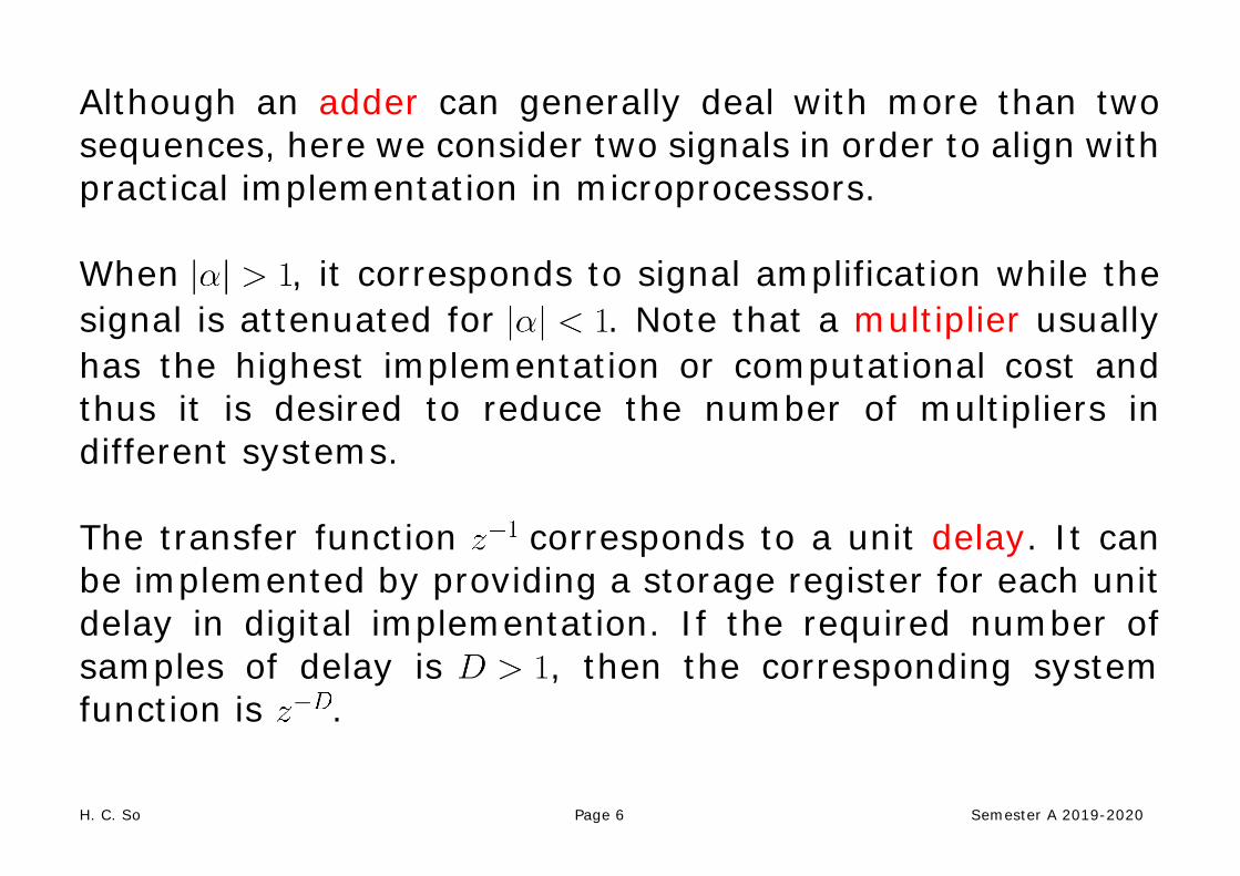
Although an adder can generally deal with more than two sequences, here we consider two signals in order to align with practical implementation in microprocessors. When , it corresponds to signal amplification while the signal is attenuated for . Note that a multiplier usually has the highest implementation or computational cost and thus it is desired to reduce the number of multipliers in different systems. The transfer function corresponds to a unit delay. It can be implemented by providing a storage register for each unit delay in digital implementation. If the required number of samples of delay is , then the corresponding system function is .
H. C. So Page 7 Semester A 2019-2020
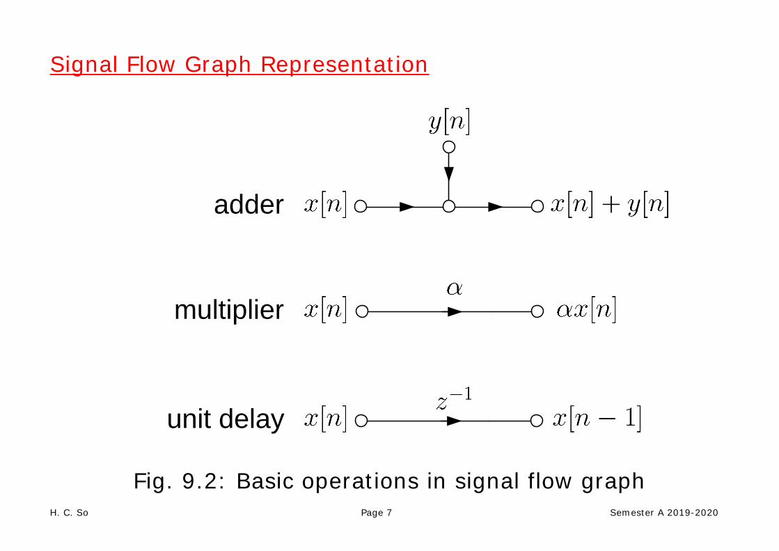
Signal Flow Graph Representation
adder
multiplier
unit delay
Fig. 9.2: Basic operations in signal flow graph

H. C. So Page 8 Semester A 2019-2020
Its basic elements are branches with directions, and nodes. That is, a signal flow graph is a set of directed branches that connect at nodes.
Signal at a node of a flow graph is equal to the sum of the signals from all branches connecting to the node.
Signal out of a branch is equal to the branch gain times the signal into the branch. Branch gain can refer to a scalar or a transfer function of corresponding to multiplication or unit delay operation, respectively. When the branch gain is unity, it is left unlabeled.
A signal flow graph provides an alternative but equivalent graphical representation to a block diagram structure
H. C. So Page 9 Semester A 2019-2020
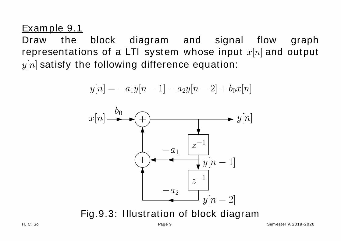
Example 9.1 Draw the block diagram and signal flow graph representations of a LTI system whose input and output
satisfy the following difference equation:
Fig.9.3: Illustration of block diagram
H. C. So Page 10 Semester A 2019-2020
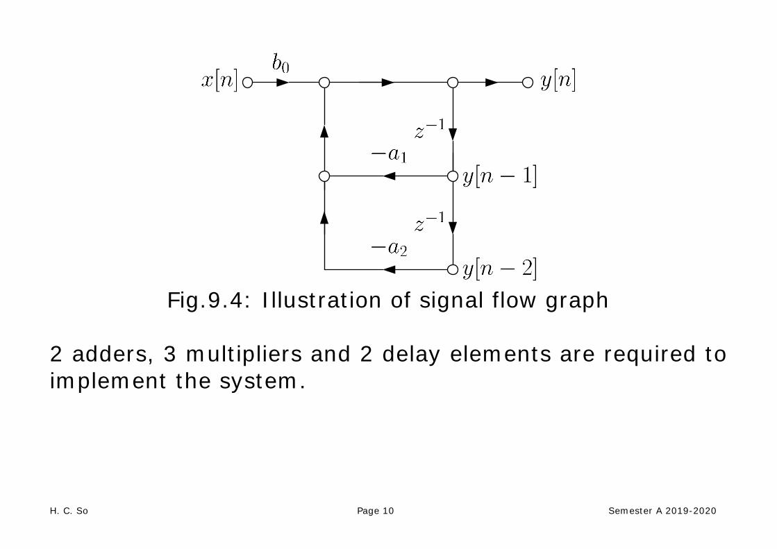
Fig.9.4: Illustration of signal flow graph
2 adders, 3 multipliers and 2 delay elements are required to implement the system.

H. C. So Page 11 Semester A 2019-2020
Structures for FIR Filter
For FIR filter, its transfer function does not contain pole. That is, setting and in (9.1) yields a FIR system:
(9.5)
while the corresponding difference equation is:
(9.6)

H. C. So Page 12 Semester A 2019-2020
1. Direct Form
Comparing (9.6) with the convolution formula of (3.20), correspond to the system impulse response : (9.7)
(9.6) can also be written as:
(9.8)
The direct form follows straightforwardly from the difference equation.

H. C. So Page 13 Semester A 2019-2020
The implementation needs memory locations for storing previous inputs of , multiplications and additions for computing each output value of .
Fig.9.5: Direct form of FIR filter

H. C. So Page 14 Semester A 2019-2020
2. Cascade Form
Expressing (9.5) as products of second-order polynomial system functions via factorization:
(9.9)
where is the largest integer contained in
. Note that when is odd, one of the will be zero. Assuming that is even, this implementation needs storage elements, multiplications and additions, for computing each output value of . Why second-order polynomial instead of first-order polynomial?

H. C. So Page 15 Semester A 2019-2020
Fig.9.6: Cascade form of FIR filter (9.10) and (9.11)

H. C. So Page 16 Semester A 2019-2020
Taking transform on (9.10) and (9.11):
(9.12) and
(9.13)
Substituting (9.13) into (9.12) yields:
(9.14) Extending (9.14) to , we finally get:
(9.15)

H. C. So Page 17 Semester A 2019-2020
To save the computational complexity, we express (9.9) as:
(9.16)
where , and ,
. That is, all are normalized to 1. Assuming that is even, (9.16) needs delay elements,
multiplications and additions, for computing each output value of
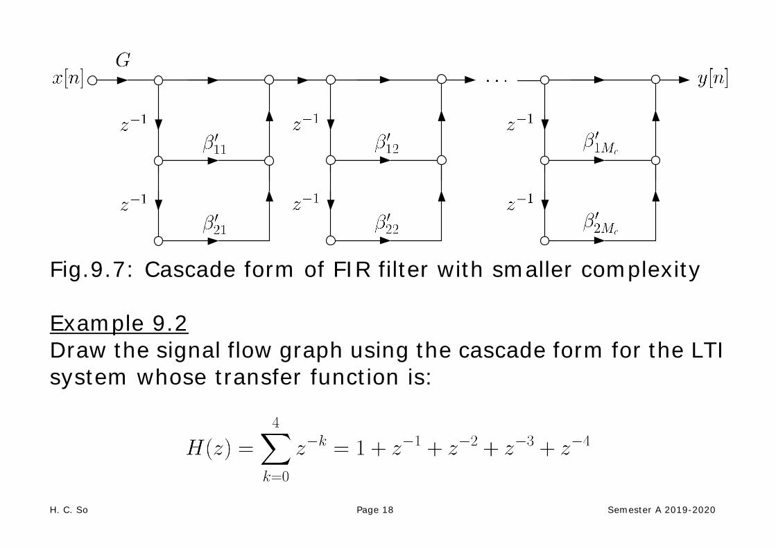
H. C. So Page 18 Semester A 2019-2020
Fig.9.7: Cascade form of FIR filter with smaller complexity Example 9.2 Draw the signal flow graph using the cascade form for the LTI system whose transfer function is:

H. C. So Page 19 Semester A 2019-2020
To factorize , we use the MATLAB command roots([1 1 1 1 1]) to solve for the roots:
0.3090 + 0.9511i 0.3090 - 0.9511i -0.8090 + 0.5878i -0.8090 - 0.5878i Hence can be factorized as
Although it can be realized with first-order sections, complex coefficients are needed, which implies higher computational cost. To guarantee real-valued coefficients, we group the sections of complex conjugates together:

H. C. So Page 20 Semester A 2019-2020
Fig.9.8: Two possible cascade forms for FIR filter

H. C. So Page 21 Semester A 2019-2020
Structures for IIR Filter
When there is at least one pole in , it corresponds to an IIR filter. The corresponding transfer function is thus:
(9.17)
Note that IIR filter is the general form of any discrete-time LTI system.
H. C. So Page 22 Semester A 2019-2020
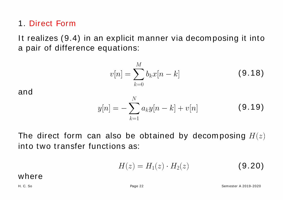
1. Direct Form
It realizes (9.4) in an explicit manner via decomposing it into a pair of difference equations:
(9.18)
and
(9.19)
The direct form can also be obtained by decomposing into two transfer functions as: (9.20) where

H. C. So Page 23 Semester A 2019-2020
(9.21)
and (9.22)
In the transform domain, we have:
(9.23)
and (9.24)

H. C. So Page 24 Semester A 2019-2020
Fig.9.9: Direct form of IIR filter

H. C. So Page 25 Semester A 2019-2020
The direct form implementation needs memory locations, multiplications and additions, for computing each output value of . 2. Canonic Form
On the other hand, we can first pass through the filter to produce an intermediate signal . The is then
passed through the system to give :
(9.25)
and
(9.26)
H. C. So Page 26 Semester A 2019-2020
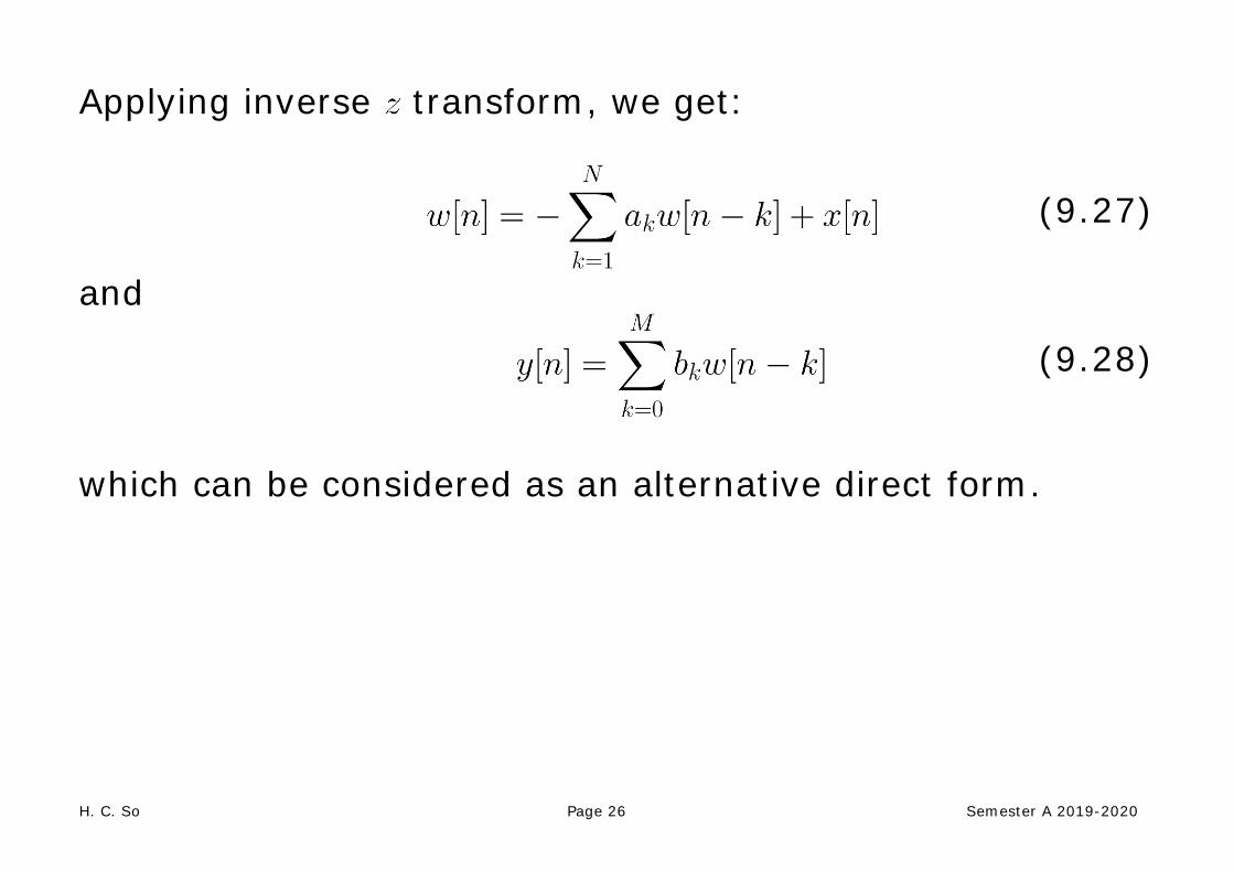
Applying inverse transform, we get:
(9.27)
and
(9.28)
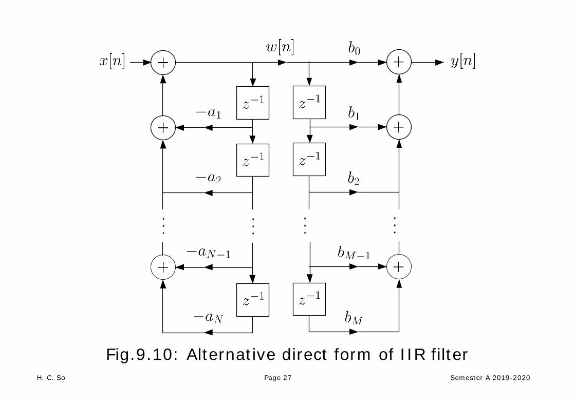
which can be considered as an alternative direct form.
H. C. So Page 27 Semester A 2019-2020
Fig.9.10: Alternative direct form of IIR filter

H. C. So Page 28 Semester A 2019-2020
Assume . Since the same signals , are stored in the two chains of
storage elements, they can be combined to reduce the memory requirement. In general, the minimum number of delay elements required is . It is called canonic form because this implementation involves the minimum number of storages.

H. C. So Page 29 Semester A 2019-2020
Fig.9.11: Canonic form of IIR filter
H. C. So Page 30 Semester A 2019-2020
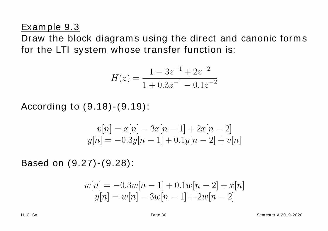
Example 9.3 Draw the block diagrams using the direct and canonic forms for the LTI system whose transfer function is:
According to (9.18)-(9.19):
Based on (9.27)-(9.28):
H. C. So Page 31 Semester A 2019-2020
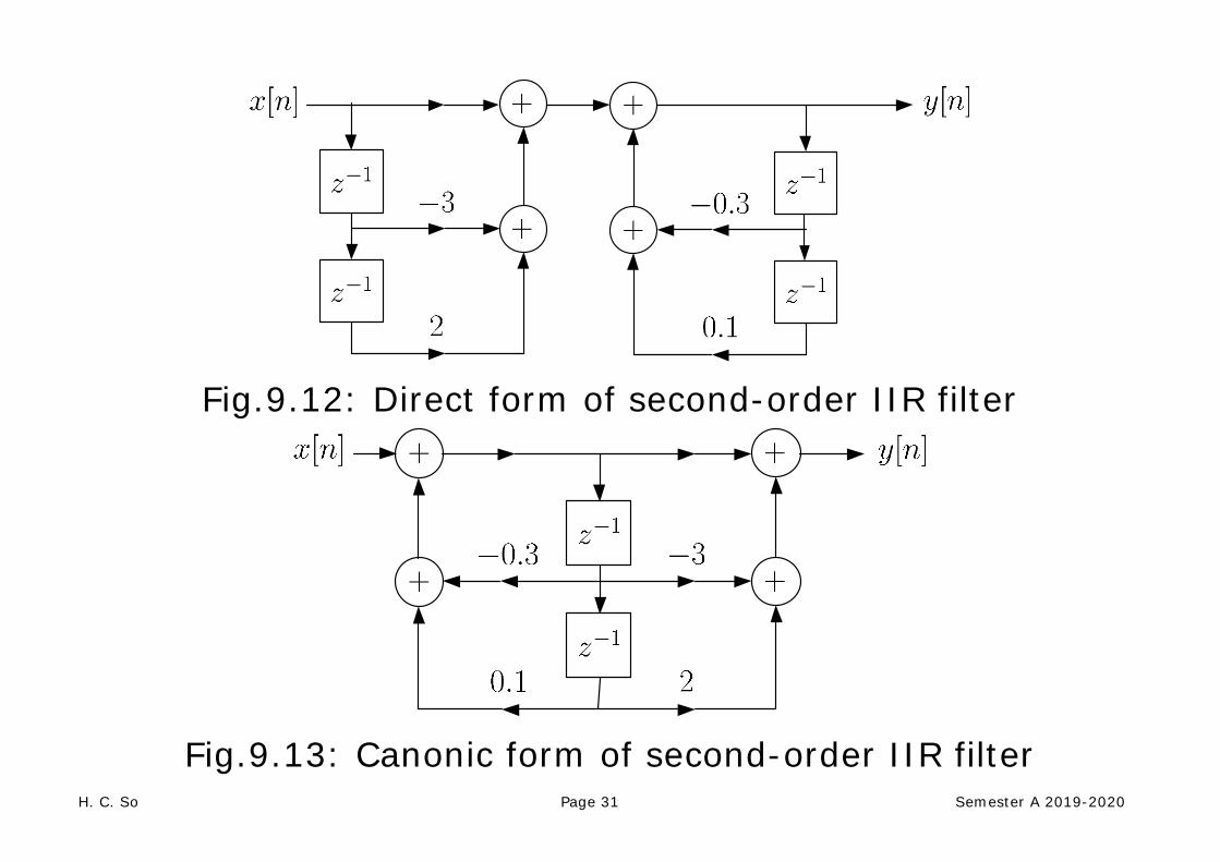
Fig.9.12: Direct form of second-order IIR filter
Fig.9.13: Canonic form of second-order IIR filter

H. C. So Page 32 Semester A 2019-2020
3. Cascade Form
We factorize the numerator and denominator polynomials in terms of second-order polynomial system functions as:
(9.29)
Without loss of generality, it is assumed that so that
. Note that when or is odd, one of the or will be zero.
H. C. So Page 33 Semester A 2019-2020
Each second-order subsystem
(9.30)
can be realized in either the direct or canonic form. Nevertheless, the canonic form is preferred because it requires the minimum number of delay elements. In IIR filter implementation, we can group the numerator and denominator of (9.30) in different ways, leading to different pole and zero combinations in each of the second-order sections. For example, there are four possible cascade realizations for a fourth-order IIR filter with .
H. C. So Page 34 Semester A 2019-2020

H. C. So Page 35 Semester A 2019-2020
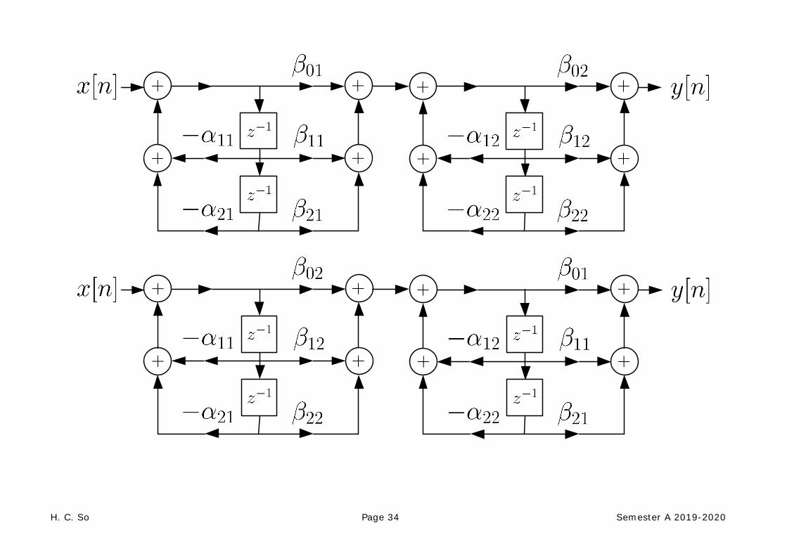
Fig.9.14: 4 possible cascade realizations for 4th-order IIR filter

H. C. So Page 36 Semester A 2019-2020
To save the computational complexity, we express (9.29) as
(9.31)
where , and ,
. Assuming that is even with , the cascade implementation of (9.31) needs or delay elements,
multiplications and additions, for computing each . That is, its memory and computational requirements are
equal to those of the direct or canonic form.

H. C. So Page 37 Semester A 2019-2020
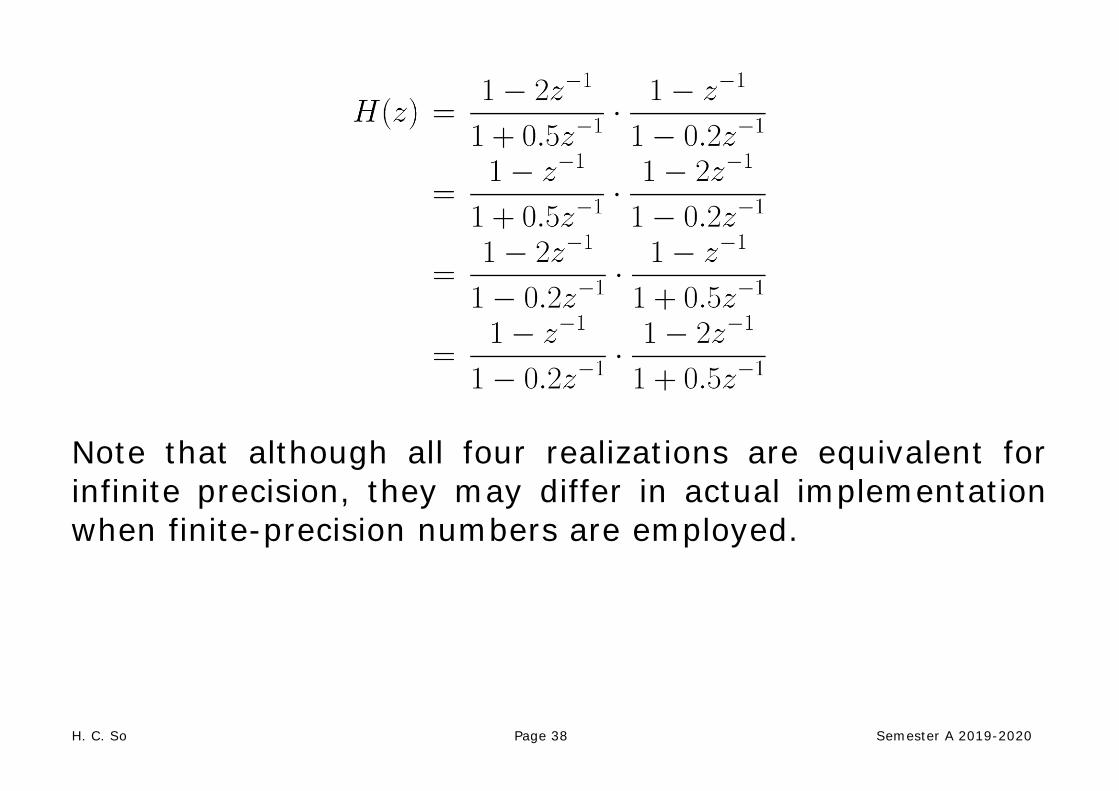
Example 9.4 Draw the signal flow graph using the cascade form with first-order sections for the LTI system whose transfer function is:
For each first-order section, canonic form is assumed. Solving the quadratic equations of the numerator and denominator polynomials, we can factorize as:
There are four possible cascade forms for :
H. C. So Page 38 Semester A 2019-2020
Note that although all four realizations are equivalent for infinite precision, they may differ in actual implementation when finite-precision numbers are employed.

H. C. So Page 39 Semester A 2019-2020
Fig.9.15: 4 possible cascade realizations with 1st-order sections
H. C. So Page 40 Semester A 2019-2020
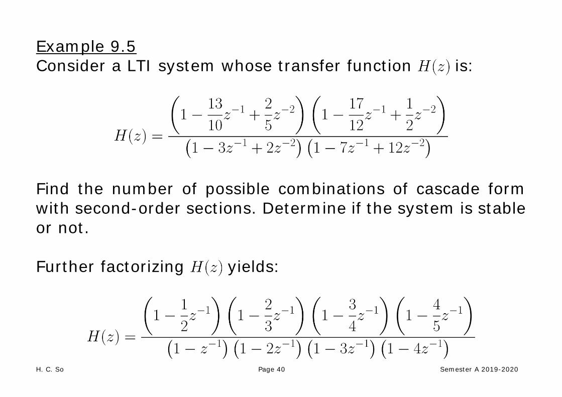
Example 9.5 Consider a LTI system whose transfer function is:
Find the number of possible combinations of cascade form with second-order sections. Determine if the system is stable or not. Further factorizing yields:

H. C. So Page 41 Semester A 2019-2020
For the numerator polynomials, there are 3 grouping possibilities in terms of second-order sections as follows:
There are also 3 grouping possibilities for the denominator:
H. C. So Page 42 Semester A 2019-2020
Each fourth-order IIR filter can be realized in four possible cascade forms. As a result, the number of possible cascade form combinations with second-order sections for is
. When implementing a filter, causality is always assumed because it is impossible to realize a noncausal system where the output depends on future input. It is clear that the region of convergence (ROC) for causal is . Since the ROC does not include the unit circle, the system is not stable. In summary, a causal system is stable when all poles are inside the unit circle.

H. C. So Page 43 Semester A 2019-2020
4. Parallel Form
The idea of the parallel form is similar to the partial fraction expansion of transform:
(9.32)
where . But now we use second-order sections in order to ensure all , , and are real. Note that when , the first summation term in (9.32) will not be included.
H. C. So Page 44 Semester A 2019-2020
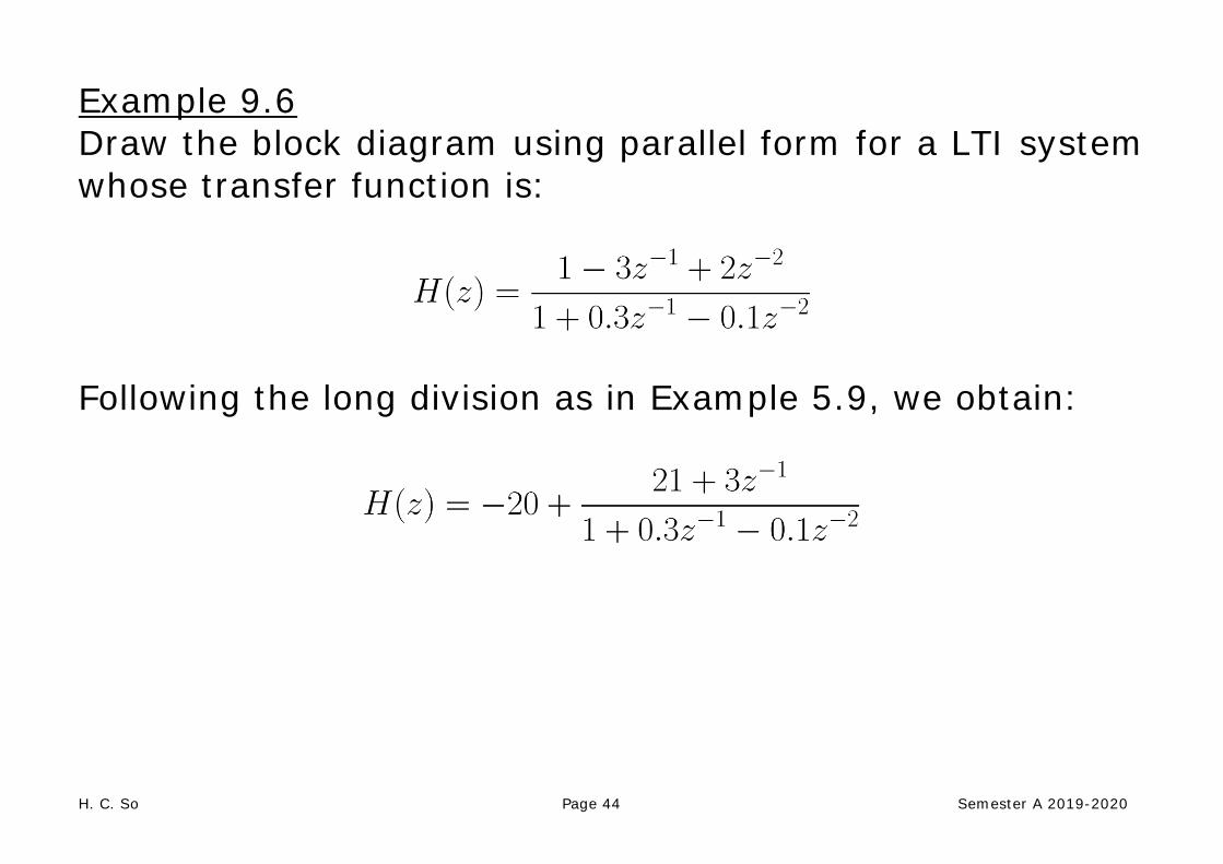
Example 9.6 Draw the block diagram using parallel form for a LTI system whose transfer function is:
Following the long division as in Example 5.9, we obtain:

H. C. So Page 45 Semester A 2019-2020
Fig.9.16: Parallel form with second-order section
As the poles of are real, we can also express in terms of first-order sections as:

H. C. So Page 46 Semester A 2019-2020
Fig.9.17: Parallel form with first-order sections

H. C. So Page 47 Semester A 2019-2020
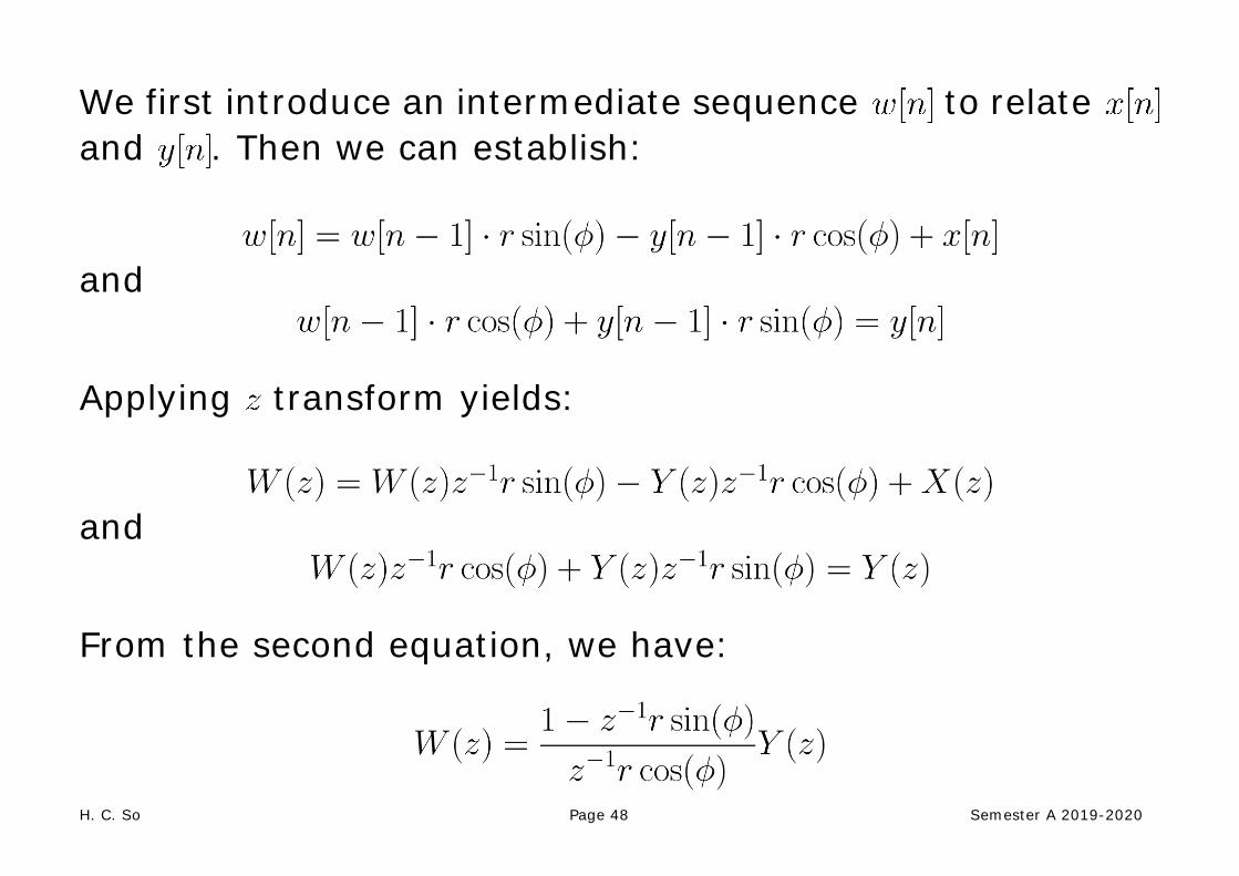
Example 9.7 Determine the transfer function and the difference equation which relates and for
Fig.9.18: LTI system parameterized by and
H. C. So Page 48 Semester A 2019-2020
We first introduce an intermediate sequence to relate and . Then we can establish:
and
Applying transform yields:
and
From the second equation, we have:

H. C. So Page 49 Semester A 2019-2020
Substituting it into the first equation, we finally have:
Taking the inverse transform gives:

H. C. So Page 50 Semester A 2019-2020
Comparison of Different Structures
The major factors that affect our choice of a specific realization are computational complexity, memory requirement, and finite word-length effects. Assuming that
is even with :
Structure Multiplication Addition Register Direct form Cascade form
Table 9.1: FIR filter structure comparison
Structure Multiplication Addition Register Direct form Canonic form Cascade form Parallel form
Table 9.2: IIR filter structure comparison

H. C. So Page 51 Semester A 2019-2020
Computations of the direct form can be reduced if the FIR filter coefficients are symmetric or anti-symmetric.
When the filter coefficients are expressed using infinite precision numbers, all realizations are same. However, in practice, they are processed in registers which have finite word-lengths. In the presence of quantization errors, the cascade and parallel realizations are more robust than the direct and canonic forms, that is, they have frequency responses closer to the desired responses.
FIR filters are less sensitive than IIR filters to finite word-length effects.
For a feasible system, it should be causal and stable.
In cascade and parallel realizations of IIR filters, system stability can be easily monitored by checking pole locations.