REALIZABLE PRODUCT LINE DESIGN OPTIMIZATION:

COORDINATING MARKETING AND ENGINEERING MODELS VIA

ANALYTICAL TARGET CASCADING

Jeremy J. Michalek

Fred M. Feinberg

Feray Adiguzel

Peter Ebbes

Panos Y. Papalambros Under review at Marketing Science. Please do not quote or distribute without prior consent. Fred Feinberg (feinf@umich.edu), Feray Adiguzel (adiguzel@bus.umich.edu) and Peter Ebbes (pebbes@bus.umich.edu), University of Michigan Business School; Jeremy Michalek (michalek@umich.edu) and Panos Papalambros (pyp@umich.edu), Department of Mechanical Engineering, University of Michigan. The authors wish to thank Jin Gyo Kim, Peter Lenk, Laura Stojan, Michel Wedel and Carolyn Yoon for their help and comments, and to acknowledge the sponsorship of the Rackham Antilium interdisciplinary project, the Reconfigurable Manufacturing Systems Engineering Research Center and the Business School, all at the University of Michigan.

1

REALIZABLE PRODUCT LINE DESIGN OPTIMIZATION:

COORDINATING MARKETING AND ENGINEERING MODELS VIA

ANALYTICAL TARGET CASCADING

ABSTRACT

We present a novel modeling and solution methodology for the product line optimization problem. Our approach formally coordinates performance models from engineering design with consumer preference models from marketing to reach joint solutions that achieve both technical and market feasibility. The methodology, based on the analytical target cascading (ATC) formulation for hierarchical systems optimization, offers rigorous integration of a number of separate modeling disciplines – conjoint analysis for preference elicitation, a Hierarchical Bayesian (HB) account of consumer heterogeneity, and physical-geometric product design models – allowing them to intercommunicate effectively. These methods are known to work well in isolation, and their joint convergence properties are assured under ATC. We show how ATC, in concert with HB conjoint, allows efficient gradient-based search of the product characteristic space relative to a posterior profit-based objective function, while ensuring technical feasibility of the product line.

The proposed methodology is illustrated through the design of a real product line, for dial-readout scales, based on a full parametric representation for products in the line and web-collected conjoint choice data. Some results of interest to both marketers and engineers are: (1) Product lines deemed as “optimal” through marketing analysis alone may not be achievable by any feasible engineering design; (2) allowing ATC to coordinate marketing and engineering models produces joint solutions superior to those using a disjoint sequential approach; and (3) for product optimization, heterogeneity matters: the form used to represent consumer heterogeneity has a substantial impact on the design (and profitability) of the resulting product line, even when designing a single product. The intrinsic modularity afforded by ATC allows ready application of alternative techniques from the choice modeling and engineering design literatures, opening new avenues for modelers and practitioners.

KEYWORDS: Product Design; Discrete Choice; Product Lines; Analytical Target Cascading; Hierarchical Bayes; Conjoint Analysis; Constrained Optimization; Design Optimization.

2

1. INTRODUCTION

It is a truism bordering on cliché that producers sell not merely isolated products, but product

lines. As such, each producer competes against both itself (cannibalization) and rivals, and must determine

how to do so effectively. The academic community has developed an array of techniques to select sets of

products that, considered jointly, optimize a given objective function, typically total profit for the line.

Marketing approaches to what has become known as the product line selection problem (Green

and Krieger 1985; McBride and Zufryden 1988) or product line design problem (Dobson and Kalish 1988;

Kohli and Sukumar 1990) have been many and varied. Certain commonalities, however, can be noted

across them: Elicitation of consumer preferences; an econometric model for mapping preferences onto

product characteristics; an explicit demand or objective function; and, linking these, an optimization

method. Searching the space of product characteristics exhaustively is often prohibitive (certain variants

are known to be NP-hard), so prior research has been devoted primarily to efficient, scalable optimization

algorithms (Chen and Hausman 2000; Steiner and Hruschka 2002). Each of the components of this body of

work is sufficiently well-developed to consider it a mature methodology, deployable when market and

product characteristics are well understood.

In the engineering community, design decision-making models typically involve maximizing a set

of performance objectives to meet a set of exogenously determined product characteristic targets subject to

technical feasibility constraints. Recently, researchers in the engineering community have begun to study

optimal product line design in the context of models of producer objectives (Li and Azarm, 2002);

however, the bulk of such efforts in engineering focus on the study of product commonality and platforms

(Simpson, 2004).

In the real world of product development, marketers and engineers face the continual challenge of

having to conform to one another’s constraints. Marketers, including those in the academic community,

predicate their methods and models on an understanding of “product characteristic space”: the

characteristics, and levels of those characteristics, which can be manipulated to attract consumers and

generate profit. In contrast, design engineers work in the “design space,” selecting values for detailed,

technical design variables in order to achieve desired target product characteristics. If engineering is

unable to design and produce a feasible product that is sufficiently close to the targets identified in the

marketing analysis, additional rounds of measurement, design and intercommunication must be

undertaken. It has been amply documented in the product development literature that this back-and-forth

passing is costly, time-consuming and, most importantly, can lead to sub-optimal final designs (Griffin and

Hauser, 1992; Krishnan and Ulrich, 2001). How this might be rectified in formal product line design

models remains an open question, and it is this question we seek to answer.

3

Creating a formal system for product line optimization must allow marketing and engineering

design models to “speak to” one another in a well-defined, efficient, and convergent manner. One

historical obstacle to achieving this objective is differences in control variables: Marketing makes use of

primary research methods, for example questionnaires and focus groups, to infer what consumers want;

that is, consumer preferences are taken as primitives. A typical approach (elaborated later in detail) is to

view products as “bundles of attributes” (McAlister 1982) and use measured consumer preferences to

locate “sweet spots” in the space of consumer-defined product characteristics. Engineers, however, do not

optimize over product characteristics themselves, but instead manipulate physically embodied design

variables to achieve performance goals. For example, what may be conveyed to a consumer as “sturdy” or

“durable” must be translated into the set of technical specifications (loading conditions, allowable

deflections, yield strength) over which engineers have control through manipulation of the design (metal

thickness, spring tension, etc.), subject to inviolable physical and geometric constraints. The interaction

between these two perspectives is largely absent from the marketing literature on product line

optimization, and formalizing this interaction is among the main contributions of the methodology

introduced in this article.

One might question why firms don’t simply integrate marketing decision-making with engineering

design and production from the outset. The conclusion of the extant literature on the topic is that there are

non-trivial impediments to such integration (e.g., Griffin, 1997; Wind and Mahajan, 1997). Hauser (2001)

highlights the difficulty of coordinating resources and agents across functional areas, each with

idiosyncratic notions of “success”, and he suggests a set of metrics for that purpose. Our goal is less one of

measurement than pragmatism: embedding marketing and engineering product line design models into a

deployable formal framework that admits of real consumer choice data and can be reliably optimized.

We present a novel approach to the product line optimization problem, one which formally links

marketing and engineering product design submodels in order to ensure feasibility of the product line

while pursuing producer objectives with respect to customer preferences. Our approach calls on proven

strengths of the models in both disciplines best suited to intercommunication and joint optimization. From

marketing, we employ Hierarchical Bayesian (HB) methods and choice-based conjoint analysis to build

data-driven discrete choice models of demand using a general representation of consumer preference

heterogeneity and capitalizing on Monte Carlo techniques. From engineering design, we utilize

engineering performance design optimization models and adapt the analytical target cascading (ATC)

methodology, developed for complex systems optimization through coordination of hierarchically

decomposed system and subsystem models (Kim et al., 2003a). ATC has proven convergence properties

and a record of successful application in automotive (Kim et al., 2003b) and architectural (Choudhary

2004) contexts. ATC coordination of existing marketing methods, such as conjoint analysis, discrete

4

choice analysis and demand forecasting, with engineering performance design optimization models allows

optimal product line designs to emerge without tedious, human-mediated iterations between marketing and

engineering design submodels, producing joint optima that are superior to those arising from independent

marketing and engineering design optimization.

We proceed by outlining key concepts and reviewing the relevant methods and literature from

both marketing and engineering product design. Because we anticipate an audience with widely varied

backgrounds and interests, this review is particularly inclusive and integrative. We then introduce ATC to

formally link models from the two disciplines and describe how to construct several alternative models of

demand for use within the ATC methodology. Finally, we demonstrate how a full product line might be

devised for a durable product of moderate complexity: a standard dial-readout bathroom scale.

1.1 Key Concepts

Throughout our development, several ideas will be called on consistently. The first is common in

engineering, though less so in marketing, namely, that many design problems cannot be cured solely by

capital. Simply put, some designs are physically infeasible, given current technology and a particular

product topology, and so not all desirable combinations of product characteristics may be attainable.

Among the advantages offered by the forthcoming method is that conjoint studies can be run as if such

infeasible combinations of product characteristics didn’t exist; ATC can be used post hoc not merely to

avoid deeming them optimal, but to navigate the design space around them successfully.

The second idea is that the interrelations among even simple engineering design variables can be

sufficiently complex as to prevent practical description when mapped to the domain of consumer-oriented

product characteristics. For example, in the dial-readout scale case study presented later, an increase in

weight capacity can be achieved by changing lever or pivot dimensions or by changing spring or pinion

properties, each of which affects other product characteristics in different ways. As such, the feasible

region of the product characteristic space may be difficult to describe mathematically, even if the feasible

region in the design space is relatively simple. Pre-restricting conjoint experiments only to feasible

combinations of product characteristics in a continuous space is often a practical impossibility; however,

the methodology presented here can optimize product characteristics while ensuring engineering design

feasibility without the need to explicitly map physical constraints on the design variables into the product

characteristic space.

A third idea is a linchpin of marketing theory and practice: Heterogeneity matters. However, in

contrast to some recent findings suggesting that one can be agnostic about the form of heterogeneity, so

long as it is reasonably general and not overly parsimonious (Wedel et al., 1999; Andrews, Ainslie and

5

Currim, 2002; Andrews, Ansari and Currim, 2002), our results indicate that the particular form of

heterogeneity is critical in product line optimization. Use of an aggregate or a discrete mixture model for

demand – aside from representing observed choices less ably – results in product line solutions differing

from those arising from a more general mixture model allowing for continuous within-class heterogeneity.

While one might assume that a homogeneous model is sufficient for design of a single product, we find

that even single-product solutions depend critically on heterogeneity correction.

The final idea is a mainstay of research on product design across different functional areas:

Iterative communication is crucial (Brown and Eisenhardt, 1995; Leenders and Wierenga, 2002). Design

submodels from marketing and engineering design must feed into one another, allowing an iterative path to

joint convergence. Our empirical application will suggest that a disjoint scenario, in which engineering

design optimization simply follows targets obtained through marketing line optimization, produces inferior

results to those afforded by the intrinsically iterative ATC-based approach.

A key to understanding the ATC approach is that it is, at base, a method for coordinating various

models; in our case, those models are drawn from engineering and marketing. As such, it is not intended to

reinvent the basic models in marketing and engineering developed over many decades, but rather to allow

them to intercommunicate without reconstructing them from the ground up. ATC “advocates” that

members of an interdisciplinary team bring the best their own modeling traditions can offer, allowing the

formal framework to coordinate them towards a jointly satisfactory optimum.

1.2 Marketing Literature

Among the core distinctions in Kaul and Rao’s (1995) comprehensive review of the marketing

product optimization literature is that between marketing positioning models, which concern abstract

perceptual attributes, and marketing design models, which set optimal levels of measurable product

characteristics. We will retain this distinction between attributes as perceived subjective qualities and

characteristics as measured objective quantities: “high-readability” is an attribute, “1.75 inch numbers” a

characteristic. We will focus on characteristics to as great an extent possible, as these can be affected

directly through design decisions, and we leave the incorporation of psychophysical mappings to

perceptual attributes as future work.

The product line optimization literature in marketing is largely concerned with setting product

characteristic and price levels to maximize profit, sales or share. This is typically accomplished by

coupling formal methods of non-linear and discrete optimization with value/utility measurement

techniques such as conjoint analysis. Among the earliest work in this vein was Zufryden (1977), who

applied integer programming to optimal design, and Green and Krieger (1985), who subsequently showed

6

how to extend existing single product design optimization heuristics to entire lines. The general product

line optimization problem was rendered into what might be called its current form by Dobson and Kalish

(1988) and by McBride and Zufryden (1988), who considered a known set of related or substitute products

and asked how their characteristics can be optimally set by a monopolist to maximize some criterion of

interest, ordinarily line profit. A great deal of subsequent research sought computationally efficient

algorithms to pinpoint the “best” product (or set of products) from all available candidates, usually via

dynamic programming (Kohli and Sukumar, 1990; Dobson and Kalish, 1993). Among the most recent

methods is that of Steiner and Hruschka (2002) who adopt genetic algorithms to efficiently locate near-

optimal product line designs.

A mainstay of product line optimization research is conjoint analysis (Green and Rao, 1971;

Louviere, 1988; Kaul and Rao 1995), the dominant approach to measuring “consumer value systems” by

applying efficient statistical experimental design techniques to survey design. Conjoint is ubiquitous in

marketing theory and practice, and has been used in the design of thousands of products across the world

(Wittink and Cattin, 1989; Wittink et al., 1994). Much recent work focuses on the accurate representation

of consumer heterogeneity, with a growing consensus in favor of Hierarchical Bayes (HB) formulations

(Lenk et al., 1996; Allenby and Rossi, 2003), which we adopt here.

Like Chen and Hausman (2000), we invoke a number of assumptions to focus on product line

optimization issues; specifically: that the total potential market size can be (exogenously) determined; that

each customer purchases either zero or one product from the line; that a customer’s purchase decision is

not overtly influenced by those of other customers; and that production can be scaled up or down as

needed to suit demand. Our formulation is well-suited to stable, durable goods categories, which comprise

the majority of line optimization decisions. It is arguably less appropriate for rapidly-developing product

classes (e.g., high-tech products), contexts lacking models to describe technical/engineering design

tradeoffs, or those where aggregate demand is erratic. Unlike Chen and Hausman (2000) or other prior

research in the area, we invoke only mild parametric assumptions about how to represent consumer

preferences. Indeed, one of the main attractions of our approach is a fully Bayesian account of a most

general form of preference heterogeneity and a method for line optimization conditional upon it. And,

unlike prior work in marketing, we provide a framework for dealing with technologically “unachievable”

product combinations, treating them as an integral part of the modeling formulation.

Steiner and Hruschka (2002) classify profit optimization methods into “one step” and “two step”

types. The former optimize directly over product lines as described by part-worth values and an objective

(profit) function; the latter, to reduce combinatorial complexity, first reduce of the full set of potential

products before optimizing. Generally speaking, culling the full set to “promising candidates” is non-

trivial, and we follow Kohli and Sukumar (1990), searching the entire product space without prior

7

restrictions or processing. However, we mitigate the discrete nature imposed by the form of conjoint data

(characteristics discretized into levels) via individual-level spline interpolation. While the resulting “profit

surface” can be complex, it is locally smooth and continuous, allowing for efficient gradient-based

nonlinear programming algorithms and ensuring that ATC will converge (Michelena et al. 2003; Michalek

and Papalambros 2005), typically in a reasonable amount of time.

1.3 Engineering Design Literature

By contrast to the marketing literature, the bulk of the engineering design literature relevant to

product line design focuses on the study of product commonality and product platforms (Simpson, 2004;

Kokkolaras et al., 2002). There exists a rich and well-developed literature on design optimization, which

focuses on setting design variables to achieve desired product characteristic targets (typically maximizing

performance) for a single product subject to physical constraints (see Papalambros and Wilde 2000 for a

comprehensive overview). When optimizing over multiple conflicting objectives, a Pareto set of non-

dominated solutions exists, and unambiguous selection of a single design from that set requires expression

of preferences in the tradeoffs among objectives. Research in multiobjective optimization offers methods

to explore this set and choose tradeoff points, typically based on designer intuition.

Recently, frameworks have been proposed in the engineering design community (e.g., Hazelrigg,

1988, Georgiopoulos, 2003) that attempt to resolve technical tradeoffs via formal models of how the firm’s

financial objectives are affected by engineering design decisions and uncertainty in those decisions. A

number of variants and implementations of the basic framework have been proposed (for example,

Marston and Mistree, 1998; Wassenaar and Chen, 2003). In particular, Li and Azarm (2000, 2002) propose

a two-step approach, first generating a set of designs that are Pareto-optimal in performance and then

selecting a product line from that set based on a “first choice” model of demand using stochastic

algorithms. This sequential approach can be effective for product line design cases where preferences for

product characteristics are strictly monotonic across the consumer population (e.g., fuel economy,

reliability, etc.) because in these cases the same Pareto set is relevant to all consumers, and individuals

differ only in their preferred tradeoff among the competing performance objectives. In our example, dial-

readout scales, no such universal Pareto set exists because different consumers have different ideal points

for size, shape, and other valued attributes.

Another area of engineering design research, Multidisciplinary Design Optimization (MDO),

offers a host of methods for decomposing complex engineering systems involving multiple simulations

into subproblems and coordinating solutions to the subproblems in order to make solving the overall

system more manageable, reliable, or efficient (Balling and Sobieski, 1994). MDO methods have been

applied primarily to coordinate engineering models in aerospace design; however, Gu et al. (2002) used

8

the Collaborative Optimization (CO) technique to propose a framework for decomposing and coordinating

separate marketing and engineering models for the design of a single product. In our approach, by contrast,

a hierarchy of product planning and engineering design models are coordinated to design a product line

using ATC, which is proven to converge to joint solutions for arbitrarily large hierarchies (Michelena et

al., 2003; Michalek and Papalambros, 2005). Also unlike prior approaches in engineering design, we

develop explicit econometric models of consumer preference distributions and consequent a heterogeneous

mixture model of demand conditional on actual survey choice data.

1.4 Outline of Proposed Methodology

The proposed product line design methodology entails three stages: First, consumers choose

among products in a conjoint setting; second, heterogeneous demand models are estimated, with

preference coefficients interpolated using splines; and third, ATC coordinates optimization over the space

of feasible product designs to yield optimal feasible product characteristics. The first two stages are viewed

as preprocessing for the ATC model, as shown schematically in Fig. 1 with symbols rigorously defined

later in the text. We proceed by defining the ATC methodology in Section 2, conditional on a model to

predict demand; next we describe three alternative discrete choice demand model specifications in Section

3; and finally, we demonstrate the methodology with an application to dial-readout scales in Section 4 and

discuss results in Section 5.

2. ATC COORDINATION OF MARKETING AND ENGINEERING MODELS

The ATC-based methodology presented here calls on established modeling traditions in

engineering design and marketing. It is innovative in terms of formally coordinating them and does not

seek to “reinvent the wheel” in either case. Indeed, this modularity is among its chief strengths.

ATC was conceived as a broad platform for large-scale engineering systems optimization. By

viewing a system as a decomposable hierarchy of interrelated subsystems, ATC allows each subsystem to

be modeled and optimized separately, coordinated, and then iteratively re-optimized (Kim 2001). ATC

requires a mathematical model of each subsystem, and the modeler’s task is to organize the various

subsystem models into a hierarchy, where each element in the hierarchy represents a (sub)system that is

optimized to match targets passed from the parent (super)system while setting targets that are attainable by

subsystem child elements. For example, a personal computer could be decomposed into systems such as

motherboard, power supply, and magneto-optical drives; the motherboard could be decomposed into

subsystems such as the processor, memory and expansion slots; and so on. Although we study a relatively

simple durable product, ATC has been applied to very complex products, including automotive systems

(Kim et al., 2002, 2003b), architectural systems (Choudhary 2004), and product families (Kokkolaras et

9

al., 2002), as well as to coordinating marketing and engineering models to design a single product for a

homogeneous market (Michalek et al., 2005). It is known that, using a formal iterative process called a

coordination strategy, ATC will converge to the same solution as the non-decomposed problem

(Michelena et al., 2003; Michalek and Papalambros, 2005) – in this case, the single combined optimization

problem statement including all marketing and engineering variables and functions. In practice, the non-

decomposed problem is typically far more difficult to solve, sometimes impossibly so because it often

suffers from high dimensionality and scaling difficulties and it requires modeler expertise in all areas. In

such cases, ATC provides a practicable methodology for optimizing the complex hierarchical systems

typically encountered in engineering product design.

The key idea behind our application of ATC is taking the joint marketing-engineering design

problem and (formally) decomposing it into interrelated subproblems, which can then intercommunicate

and algorithmically iterate. In general, ATC can accommodate an arbitrarily large hierarchy of marketing

and engineering subproblem elements, where parent elements set targets for child elements. For example,

the engineering design subproblem could be decomposed into a set of systems, subsystems, and

components (Kim, 2001), or the marketing subproblem could be decomposed into separate subproblems,

say, for pricing, product, positioning, packaging, and promotion. However, in this article we present only

the base case where a single “marketing subproblem” that plans the product line is coordinated with a set

of “engineering design subproblems,” one for each product in the line. An informal depiction of this

process appears in Figure 2: The marketing subproblem involves determining price and (target) product

characteristics for the full product line to maximize a known objective function, which can be profit or

some other measure of interest to the firm, without deviating too much from the feasible design achieved

by engineering, while each “engineering design subproblem” requires determining a feasible design – one

conforming to known constraints – that hews as closely as possible to product characteristic targets set in

the marketing subproblem. Decomposition into the ATC structure can be even more important in the

product line case than in the single product case explored by Michalek et al. (2004) because including

engineering models for the design of multiple products in a single optimization statement creates a high-

dimensional, highly constrained space, whereas with ATC decomposition of the line, the space of each

engineering subproblem (each product design) remains unchanged as new products are added to the line.

The marketing product planning subproblem differs from that in typical marketing applications in

one critical way: Supposedly “optimal” product characteristics and price must be associated with a product

that can be achieved by a feasible engineering design. The engineering design subproblems differ from

those in typical engineering design applications in that no arbitrary weights need be assigned to specify

multiobjective optimization tradeoffs in each of the engineering design subproblems: Instead, they are

resolved by iteratively optimizing to meet product characteristic targets set by marketing. It is the interplay

10

of minimizing deviations between target and achieved characteristics while pursuing a management goal

(profit maximization) that ATC formalizes through iteration. It bears especial mention that iteration

between groups of real people – as opposed to mathematical subproblems – entails substantial fiscal and

opportunity costs, both of which ATC helps avoid.

The chief organizational benefit of ATC is that it segregates models by discipline: Marketers can

build submodels based on, say, conjoint analysis and new product demand forecasting, engineers can

formulate models for product design and production, and other functional groups can focus on what they

know how to do well. No functional area need become an expert in modeling the others, since ATC

coordinates models with well-defined interfaces. The following sections lay out the engineering design and

marketing design subproblems explicitly, and a nomenclature table is provided at the end of this article to

summarize the notation.

2.1 ATC Marketing Subproblem

The marketing subproblem objective is to maximize profit Π with respect to the price pj and the vector of

real-valued product characteristic targets zMj for each product j in the product line j = 1,2,...,J while

minimizing deviation from the characteristics of the feasible design achieved by engineering zEj. Here the

vectors of product characteristics z represent objective, measurable aspects of the product observed by the

customer and resulting from engineering design decisions. Although firms can specify arbitrarily

sophisticated profit functions based on their experience, internal accounting and historical demand, we

eschew obfuscation by adopting a simple profit (Π) formulation – revenue minus cost – so that

( )( )V I1

Jj j j jj

p c q c=

Π = − −∑ , (1)

where pj is the (retail) price of product j, cVj is the unit variable cost of product j, cI

j is the investment cost

for product j, which represents all costs of setting up a manufacturing line for product j, and qj is quantity

of product j sold (demand), which is a function of the product characteristics zMj′ and price pj′ of all

products j′ = 1,2,...,J. We presume that product commonalities enabling investment cost sharing and

improving economies of scale do not exist, so each new product design requires new manufacturing

investment. In general, cVj and cI

j can be considered functions of market conditions or engineering

decisions, although for clarity we take them as constants. Given a demand model to calculate qj as a

function of the vector of (target) product characteristics zMj and price pj for all products j in the line, which

will be developed in the next section, the profit function is fully defined; however, the objective function

also involves minimizing deviation from the characteristics of the feasible design achieved by engineering

zEj, which are held constant while solving the marketing subproblem. This deviation for each product j is

11

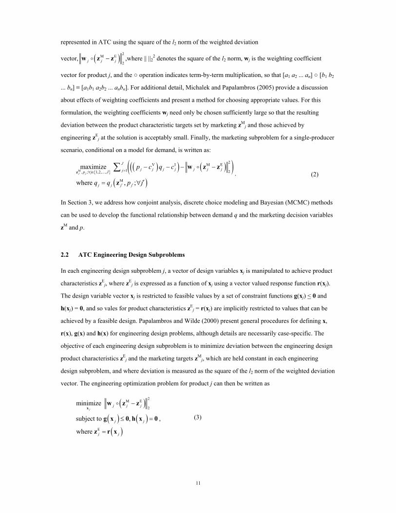
represented in ATC using the square of the l2 norm of the weighted deviation

vector, ( ) 2M E

2j j j−w z z ,where || ||22 denotes the square of the l2 norm, wj is the weighting coefficient

vector for product j, and the operation indicates term-by-term multiplication, so that [a1 a2 ... an] [b1 b2

... bn] ≡ [a1b1 a2b2 ... anbn]. For additional detail, Michalek and Papalambros (2005) provide a discussion

about effects of weighting coefficients and present a method for choosing appropriate values. For this

formulation, the weighting coefficients wj need only be chosen sufficiently large so that the resulting

deviation between the product characteristic targets set by marketing zMj and those achieved by

engineering zEj at the solution is acceptably small. Finally, the marketing subproblem for a single-producer

scenario, conditional on a model for demand, is written as:

( )( ) ( )( )

( )M

2V I M E1 2, ; 1,2, ,

M

maximize

where , ;j j

Jj j j j j j jjp j J

j j j j

p c q c

q q p j

=∀ ∈

′ ′

− − − −

′= ∀

∑z

w z z

z

… . (2)

In Section 3, we address how conjoint analysis, discrete choice modeling and Bayesian (MCMC) methods

can be used to develop the functional relationship between demand q and the marketing decision variables

zM and p.

2.2 ATC Engineering Design Subproblems

In each engineering design subproblem j, a vector of design variables xj is manipulated to achieve product

characteristics zEj, where zE

j is expressed as a function of xj using a vector valued response function r(xj).

The design variable vector xj is restricted to feasible values by a set of constraint functions g(xj) < 0 and

h(xj) = 0, and so vales for product characteristics zEj = r(xj) are implicitly restricted to values that can be

achieved by a feasible design. Papalambros and Wilde (2000) present general procedures for defining x,

r(x), g(x) and h(x) for engineering design problems, although details are necessarily case-specific. The

objective of each engineering design subproblem is to minimize deviation between the engineering design

product characteristics zEj and the marketing targets zM

j, which are held constant in each engineering

design subproblem, and where deviation is measured as the square of the l2 norm of the weighted deviation

vector. The engineering optimization problem for product j can then be written as

( )( ) ( )( )

2M E

2

E

minimize

subject to ,

where

jj j j

j j

j j

−

≤ =

=

xw z z

g x 0 h x 0

z r x

, (3)

12

2.3 Complete ATC Formulation

Figure 3 conveys a mathematical description of the concepts in Figure 2, showing the flow of the ATC-

based product line optimization model for a single producer, where the number of products in the line J is

determined through a parametric study: i.e., J is held fixed during optimization, separate optimization

solutions are found for each value of J = 1,2,..., and the value of J that produces the solution with the

highest profit is selected. In the marketing product planning subproblem (Eq.(2)) vectors of characteristic

targets zMj and price pj are chosen for each product j in order to maximize profit Π (i.e., revenue minus

cost), as defined in Eq.(1). This is achieved while minimizing the deviation between the product

characteristic targets set by marketing zMj and those achieved by each engineering design zE

j. The demand

model, which will be developed in the next section, is left as a generic function in Eq.(2) and Figure 3. In

each engineering design subproblem (Eq.(3)), design variables xj are chosen to minimize the deviation

between characteristics achieved by the design zEj and targets set by marketing zM

j subject to engineering

design constraints g(x) and h(x).

3. MODELS OF PRODUCT DEMAND

This section outlines the models used to predict demand for each product as a function of the

product characteristics and prices of all products in the producer’s product line. Extra detail and

clarification is provided for methods that are well known in the marketing community but unfamiliar to the

engineering design community (see Michalek (2005) for a more detailed discussion). First, conjoint

analysis and discrete choice models are briefly reviewed. Then three different discrete choice demand

model specifications are presented. The three models differ in their assumptions about the form of the

stochastic error terms and the representation of heterogeneity. Finally, spline interpolation is invoked to

estimate utility for products with intermediate characteristic values, and a market potential is invoked to

predict demand using the choice model.

3.1 Conjoint Choice Data Collection

Conjoint analysis has a long history as a method for inferring stated consumer preferences by

applying efficient experimental design techniques to the design of surveys. Green and Krieger (1996)

concluded that, of extant methods, choice-based conjoint analysis is the best method for the extraction of

individual-level consumer preferences, and we adopt it for our application. We stress that, for the purposes

of using ATC in real design problems, we are agnostic about the specific conjoint methodology applied,

and present here a “generic” version, albeit using a sophisticated account of consumer preference

heterogeneity, as we discuss later in full. Unfamiliar readers are referred to the excellent summary articles

13

of Green and Srinivasan (1990), Green, Wind and Rao (1998) or Bohl’s (1997) comprehensive conjoint

analysis database.

In our choice-based conjoint survey, the respondent is presented with a series of questions or

“choice sets” t = 1,2,...,T. In each choice set t, the respondent is presented a set of product alternatives

j∈Jt including the option to not choose any of the product alternatives: the “no choice” option. Each choice

set contains hypothetical product (dial readout scale) profiles with the price and product characteristics of

each product set to one of the discrete levels shown in Table 1. The characteristic and price levels of the

product alternatives in each choice set are chosen to be balanced and to collect data efficiently (as per

Kuhfeld 2003, who provides a comprehensive overview). The resulting data are the observed choices that

each respondent makes in each choice set: Φijt, where Φijt = 1 if respondent i chooses alternative j in choice

set t, and Φijt = 0 otherwise. These data Φijt are then used to estimate the parameters of the demand

model for the marketing subproblem, as illustrated in Figure 1.

3.2 Discrete Choice and Random Utility Models

As is typical in marketing and economics, we adopt a utility framework (Train, 2003) for total line

demand. Many of the previous product line optimization formulations (e.g., Dobson and Kalish, 1988;

McBride and Zufryden, 1988; Li and Azarm, 2002) adopt a “first-choice” model of demand, where utility

is written as a deterministic function of the product and consumer characteristics, and the product with the

highest utility is presumed to be chosen deterministically. Here we instead adopt a random utility model

where the utility of each product to each consumer is assumed to depend on the product’s characteristics,

the consumer’s idiosyncratic preferences for those characteristics (estimated from choice data), and a

random error component. Demand follows from the sum of the probabilities for each individual choosing

each alternative. The use of a random utility model avoids the discontinuities intrinsic to the “first choice”

model and is important for generalizing the product design space to a continuous space so that efficient

gradient-based nonlinear programming optimization algorithms can be called upon.

Throughout, we refer to a set of representative individual consumers (or groups thereof) i = 1, 2,

..., I and a set of product alternatives j = 1, 2, ..., J. Individuals i are assumed to derive from each

product j some utility value uij that is composed of a deterministic component vij, which is a function of the

observable aspects of the choice scenario, and an unobservable random error component ε ij, so that uij = vij

+ ε ij . It is assumed that each individual will choose the alternative that gives rise to the highest utility, i.e.,

alternative j is chosen by individual i if uij > uij′ for all j′≠ j. The probability, Pij, that alternative j is chosen

by individual i on a particular occasion depends on the assumed error (εij) distribution. Two such

distributions are used in essentially all choice modeling work: normal and double exponential, resulting in

14

the logit and probit models, respectively. It is well-known (Amemiya 1985) that very large samples are

required to distinguish results produced by the logit and probit specifications. Each offers advantages: The

normal distribution is expedient for Bayesian computation, due to conjugacy properties; the double

exponential distribution allows a closed-form expression for Pij, which is precise and computationally

efficient for optimization.

The deterministic component of utility, vij, can be rendered as a function of observables such as

price and product characteristics, or even consumer covariates, etc. Here we limit our purview to price and

product characteristics, elements under joint marketing and engineering control. As a practical matter,

some rule is required to map characteristics into vij. Recent econometric work explores non-parametric

representations for individual-level (Kalyanam and Shively, 1998; Kim et al., 2005) or latent utility

functions (Andrews, Ainslie and Currim, 2002). In order to take full advantage of conjoint experimental

design techniques for data collection, we discretize each characteristic ζ of the real-valued characteristic

vector zMj into a set of discrete levels ω = 1, 2, ... Ωζ and adopt a main-effects model of the discrete

product characteristic levels (conjoint part-worths). It is important to account for possible non-linearities

with respect to the underlying continuous variables, and we accomplish this via spline interpolation for

intermediate values; details of this procedure are provided below. The deterministic utility νij that

individual i derives from product j is therefore written as

0 1ij i jv ζ

ζω ζωζ ωβ δΖ Ω

= ==∑ ∑ , (4)

where the binary dummy δjζω = 1 indicates alternative j possesses characteristic ζ at level ω, and βiζω is the

part-worth coefficient of characteristic ζ at level ω for individual i, estimated from the conjoint choice data

Φ. To clarify notation, in δjζω the elements of the product characteristic vector zMj are enumerated ζ = 1,

2, ... Z, and price p is included in δjζω and labeled as element ζ = 0. Note that each product characteristic ζ

is either intrinsically discrete or is discretized into Ωζ levels, ω = 1, 2, ... Ωζ . Discrete levels are used to

avoid presumptions of linearity with respect to the underlying continuous variables (e.g., a $1 price

decrease cannot be presumed to have the same effect for a $10 product and a $100 one, and preferences for

values of product characteristics cannot, in general, be assumed monotonic). Use of the main-effects

model assumes that interaction effects are negligible, as is common practice in many conjoint

applications; however, more advanced models can be used if the modeler has reason to believe that

interaction effects may be important (Louviere et al., 2000).

In using choice models, one must account for the real possibility that none of the presented

alternatives is deemed acceptable; this is accomplished through an “outside good” or “no choice option”.

This outside good is included throughout our empirical application, and it plays the vital role of ensuring

15

that the total demand for a set of undesirable or overly expensive products will be low (see Haaijer,

Kamakura and Wedel, 2001). In the absence of an outside good, consumers are forced to choose from the

inside goods, and demand depends only on differences in offered product characteristics (cf. Berry, 1994).

Throughout, we index “no choice” as alternative 0, with error εi0 and attraction value vi0 for individual i,

where v is normalized to zero (vi0 = 0; ∀i) for identification purposes.

For purposes of comparison, we present three demand models that arise from different

specifications in each of the following elements: (1) heterogeneity in the part-worth coefficients β over the

population, and (2) the distributional form of the stochastic error components of utility εij.

3.2.1 A simple homogenous specification

In the simple homogeneous case, all individuals are presumed to belong to the same segment (i.e.,

they are all presumed to have the same preference coefficientsβζω, and therefore the same deterministic

component of utility vj for a given product), so the consumer segment index i drops out. If, the stochastic

error terms εij are taken to be independent and identically distributed across products and to follow the

“extreme value” (or “double exponential”) distribution (i.e., Pr(εij<α) = -exp(-exp(-α))), then the choice

probability Pjt for product j in choice set t is given by the well-known logit expression:

j

j

t

v

jt v

j

ePe ′

′∈

=∑ I

, (5)

where vj is defined in Eq.(4), and the parameters βζω are estimated from the conjoint choice data Φ using

maximum likelihood techniques. An important shortcoming here is the assumption of homogenous

consumer preferences, which is unrealistic (Leeflang et al., 2000) when consumers differ

systematically in behavior and preferences. Failure to correctly model this heterogeneity leads to

biased parameter estimates and, consequently, suboptimal product line designs; we illustrate this

phenomenon in our empirical study. In particular, the independence from irrelevant alternatives (IIA)

property arising from the assumption of independently and identically distributed errors across

alternatives implies that the model will tend to underestimate the degree to which two highly similar

objects compete with one another (Train, 2003). This makes the homogeneous model unsuitable for

product line optimization because solutions contain duplicate products. In the following sections we

present two other models that allow for more complex patterns for heterogeneity.

16

3.2.2 A discrete mixture heterogeneity specification

The limitations of the homogeneity restriction can be addressed via the well-known discrete

mixture or latent class model (Kamakura and Russell 1989). Here we presume that there exists a fixed

number of consumer segments B, where each segment b = 1,2,...,B contains sb fraction of the population,

and individuals in segment b have identical preferences βbζω, but preferences differ between segments. The

deterministic component of utility vbj derived from product j by a member of segment b is given by Eq.(4)

using the within-segment preferences βbζω. Given an i.i.d extreme value error distribution for the error

terms ε, the unconditional choice probability Pjt of choosing product j from choice set t is now the

weighted sum:

1

bj

bj

t

vB

jt b vbj

eP se ′=

′∈

⎛ ⎞⎜ ⎟=⎜ ⎟⎝ ⎠

∑ ∑ I

, (6)

The discrete mixture model is also readily estimated from the conjoint choice data Φ using maximum

likelihood techniques (with respect to the β and sb terms). Model selection (to choose among different

values of B) can be achieved through standard measures as BIC (Kadane and Lazar, 2004).

The discrete mixture model also helps address the IIA problem, which is well-known to be

exacerbated, particularly in choice-based conjoint (CBC) models, when heterogeneity is not adequately

accounted for (Orme, 1998). Nevertheless, it is often argued that the finite mixture representation of

heterogeneity is too restrictive: an artificial partitioning into homogeneous segments (Leeflang et al., 2000;

Rossi and Allenby 2003). In particular, the IIA problem still exists within-segment, and optimal product

line solutions may contain duplicate products. If preferences are instead presumed to be continuously

distributed, results depend critically on the chosen distribution specification (Nevo, 2000; Kim et al.,

2004). In the following section we describe a model that combines both discrete and continuous

heterogeneity to approximate a wide variety of heterogeneity “shapes”.

3.2.3 A normal mixture heterogeneity specification

The heterogeneous probit model presented here includes several past conjoint choice models as

special cases (McCulloch and Rossi, 1994; Haaijer, 1999). We adopt a specification consisting of a

mixture of continuous distributions, allowing for correlated part-worth values within each mixing

component, and we explicitly test whether the correlation terms are statistically warranted (note that these

correlations are between model β coefficients, not unobserved ε error terms, which is a separate issue).

Formally, individual part-worth coefficient vectors βi, containing the elements βiζω for individual i, are

assumed to be drawn from a mixture of multivariate normal distributions, so that

17

( )1~ ,B

b b bbs N

=∑β θ Λ , (7)

where sb is the fraction of the market in “segment” (or mixing component) b. Here θb is the vector of

means for βi, and Λb is a full-variance covariance matrix (against which we can check for diagonality).

This allows for a very flexible representation, with both discrete and continuous heterogeneity (Lenk and

DeSarbo 2000). In addition, potential IIA problems are mitigated by appropriate heterogeneity correction

in that the multivariate distribution on βi has a non-diagonal covariance matrix, which serves to reduce the

impact of IIA (Nevo, 2000; or for an alternative account, see Haaijer et al. 1998).

Although the individual-level part-worth parameters βiζω for the previous models could be

obtained by maximum likelihood techniques, such an approach is impractical for the “continuous”

heterogeneity representations in this section. We instead turn to Hierarchical Bayes methods, and estimate

model parameters via Markov chain Monte Carlo (MCMC) techniques (Andrews, Ainslie, and Currim,

2002) 1. Allenby and Rossi (2003) persuasively argue for the superiority of HB-based methods over

alternative approaches to heterogeneity correction. If error terms εij are normally distributed and are

independent across individuals, alternatives and choice sets, choice probabilities Pij are described by the

probit model, which offers certain attractive conjugacy properties in a Bayesian setting, but does not yield

probabilities in closed form 2. Estimation of this particular form of probit model is facilitated through data

augmentation. The latent variables uij enable straightforward application of MCMC techniques when βi

comes from a single normal distribution. Conditionally on these latent values, the formulation is simply a

Bayesian linear model (Lenk et al. 1996, McCulloch and Rossi, 1994). Incorporation of the mixture of

normals instead of a single normal, however, does not complicate matters when a conjugate Dirichlet prior

is used for sb, because the full conditionals are also ordered Dirichlet (Lenk and DeSarbo 2000). Given

conjugate priors, the full conditional distributions can be readily derived for all model parameters (e.g.,

Rossi and McCulloch 1994, Lenk and DeSarbo 2000). Specifically, the following MCMC scheme is used:

Draw sequentially from , , , , ,ijt i b b i bu sϕΞ Ξ Ξ Ξ Ξ Ξβ θ Λ ,

where Ξ is notational shorthand for all previously sampled quantities, i.e.,uijt, βi, θb, Λb ϕi, sb, plus the

observed choice data, Φijt. Under this scheme, uijt are drawn from a truncated normal distribution; βi’s

are drawn from subject-specific multivariate normal distributions; θb is drawn form a multivariate normal

distribution; Λb is drawn from an Inverse Wishart distribution; and segment probabilities sb are drawn from

1 We are indebted to Peter Lenk for sharing both his GAUSS code and expertise.

2 As discussed above, here we use normal errors and the consequent probit model for Pj. It is in any case typically possible to post-process MCMC draws to convert between estimates obtained through various error specifications, using auxiliary Metropolis steps.

18

an ordered Dirichlet distribution. The variable ϕi is used only within the MCMC chain to draw the group

membership of individual i at each iteration, conditional on the other parameters, so that ϕi∈1,2,...,B.

We use estimates from a classical mixture of probits as starting values, and the Gibbs sampler is iterated

until a stationary posterior is obtained. To mitigate autocorrelation, we thin by retaining every 10th draw,

after a burn-in of 50,000 iterations. Convergence was examined through iteration plots. Posterior marginals

revealed no systematic convergence problems.

In order to choose among the different number of mixture components B in the mixture

representation for βi, we use the Deviance Information Criterion (DIC) statistic proposed by Spiegelhalter

et al. (1998). This method is particularly suited to complex hierarchical (Bayesian) models in which the

number of parameters is “not clearly defined” (Spiegelhalter et al. 2002). In contrast to classical methods

like AIC or BIC, the DIC statistic determines the “effective number of parameters” entailed by the model

specification itself, and so eschews calculations based on the number of parameters or observations,

likelihoods, and particular penalty functions. DIC is readily computed from standard MCMC output, and

Spiegelhalter et al. (1998) find it to perform particularly well across a variety of hierarchical models.

The model put forth thus far yields several sets of quantities, and it is helpful to take stock of them

in non-technical terms. For each survey respondent, the model offers a set of draws from (the posterior

distribution of) that respondent’s coefficients βiζω. One could then use this information for inferences about

that particular individual, or the specific set of individuals used to calibrate the model. We take a Bayesian

perspective and focus instead on parameters of the hierarchical model alone, sb, θb, Λb, which describe

the mixture distribution. These parameters can be thought of as generating the individual-level βi values,

and so are the appropriate quantities for inference and prediction.3 It is important to realize that these are

not known with certainty (i.e., sb, θb, and Λb are themselves random variables), and they possess a jointly-

specified posterior. It is this posterior over which we wish to optimize within the ATC framework. To do

so, we must integrate over the posterior choice surface arising from the MCMC chain for these

parameters.

3.3 Spline Interpolation Conditional on Generated Coefficients

The part-worth coefficient values βiζω represent individual-level preferences for each characteristic

at each discrete level used in the conjoint study. Optimizing over presumably continuously-valued product

characteristics and price requires interpolation to intermediate values. Natural cubic splines have a number

3 We generate, and optimize over, this posterior surface as follows: When the chain has stabilized, we generate new values of

βi as the chain continues to run and thin them to reduce serial correlations; specifically, we generate 10000 values and retain every 10th. The resulting set of 1000 βi draws is used to represent the population (the posterior surface) throughout the optimization. Accuracy can be enhanced if need be by generating additional βi values (although we saw

19

of desirable interpolation properties vis-à-vis optimization, particularly so near endpoints (De Boor, 2001).

We interpolate for the deterministic component of utility as a function of continuous-valued product

characteristics zj and price pj using natural cubic spline functions Ψiζ fit through the discrete levels ω =

1,2,...,Ωζ of the discrete part-worth coefficients βiζω for each individual i and each product characteristic

(plus price) ζ . Indexing characteristics as ζ = 1,…, Ζ and price as ζ = 0, the interpolated value of the

observable component of utility is

( ) ( )M0 0 1

ˆ , ,ij i i j i i jv pω ζ ζωζ ζβ βΖ

== Ψ + Ψ∑ z , (8)

where <z M j>ζ indicates the ζth element of the vector z M

j. These interpolated ijv give rise, through the

random utility specification, to expected individual choice probabilities Pij, which are summed across

individuals to generate total expected market share, as described below. It is important to realize that the

ATC methodology requires only that demand be rendered as a function of price and product characteristics

and does not hinge on a particular functional specification for this relationship. The demand surface

emerging from this entire procedure is complex, and may possess local minima.

3.4 Assessing Demand

Calculating demand involves multiplying the (unconditional) probability that a randomly selected

individual will choose product j by the market potential S. Market potential is assumed to be exogenously

determined through pre-market forecasting techniques (see Lilien et al., 1992); we take it as a given, as its

value has no effect on relative shares. To illustrate, under the logit model, demand for product j is given by

ˆ

ˆ

0

ij

ij

vi

j J vij

s eq Se ′

′=

⎛ ⎞⎜ ⎟=⎜ ⎟⎝ ⎠

∑∑

, (9)

where ijv is calculated in Eq.(8) using the spline functions derived from part-worth values. For the simple

homogeneous case, there is only one “individual” i, and si = 1. For the discrete mixture case, i indexes the

latent classes (segments), so that i = 1,2,...,B, and si is the size of segment i. For the mixture-of-normals

heterogeneity case, i refers to the draws taken from the MCMC chain, so that i = 1,2,...,ID, where ID is

the number of draws, and si = 1/ID. For a particular case, Eq.(9) can be used to specify demand in Figure 3

for ATC product line optimization coordination.4

no improvements in our empirical application by doing so). Details about the MCMC sampler, including all full conditionals, are available from the authors upon request.

4 The probit model entails Gaussian errors, so that choice probabilities must be calculated using numerical methods. In our applications, we use several such methods – quasi Monte Carlo, various types of quadrature, and a logit-based approximation (as per Amemiya, 1985) which allows direct application of Eq.(9) – finding near perfect agreement.

20

4. APPLICATION

The proof of the proposed methodology lies in its ability to design a real product line. Here, we

apply the methodology to design a line of dial-readout bathroom scales. While the methodology can be

used for durables of any type, so long as they are in a fairly stable market, scales possess several features

which make them attractive for purposes of illustration. In particular, consumers are highly familiar with

their attributes and prices, and dial-readout scales are straightforward enough that one can readily specify a

succinct list of design variables and a set of physical and geometrical constraints they need obey.

The line design problem we solve here is analogous to that of Michalek et al. (2005), who applied

ATC to optimizing a single product for a homogeneous market using logit-based demand, a far simpler

scenario. As we will show, even when a firm seeks to enter the market with a single product – a rarity

in durable product categories – the presumption of homogeneity is troublesome. ATC has not,

however, been applied before to product groups, heterogeneous markets, or in concert with Bayesian

methods. We next turn to both the marketing planning and engineering design subproblems, after which

they are formally linked via ATC.

4.1 Marketing Subproblem

To measure and predict consumer preferences, marketers must discern which aspects

(characteristics, price) of a product are most important, and which values of those characteristics are

particularly appealing. Manufacturers typically have a trove of primary data on the topic, and we presume

that they can avail of it. For example, a major scale manufacturer5 put a great deal of information at our

disposal regarding appropriate product characteristics and levels. Several of these, like color or type of

padding, were not only primarily aesthetic, but could be swapped post-production without affecting the

basic design choices addressed by the engineering design submodel; these were therefore not part of our

experimental design. Because the experiment was conducted on the web, it was crucial to convey the

nature of information prevalent in on-line product profiles. Perhaps most important was that product

characteristics be objective and tangible so that they may be objectively related to engineering design

decisions. As such, rich descriptive epithets (“attractive case”) were avoided in favor of product

dimensions and exact schematics.

Based on these considerations, five product characteristics z = [z1, z2, z3, z4, z5]T emerged as most

salient: weight capacity (z1), aspect ratio (z2), platform area (z3), tick mark gap (z4), and number size (z5), in

addition to price (p). For the conjoint study, the range of values for each characteristic was captured by

five (discrete) levels (ω = 1, 2, 3, 4, 5; Ωζ =5 ∀ζ) for the discretized conjoint dummy variables δjζω in

5 This report was proprietary.

21

Eq.(4), chosen to span at least 90% of the observed ranges for 32 sample dial-readout scales sold across

several popular web sites. Characteristics such as brand name or logo, which could be strong preference

drivers but are not central to product design decision-making, were deliberately avoided.

Respondents (n = 184) were solicited through business and engineering classes at a large

Midwestern university, as well as by internet newsgroup announcements, and entered into a sweepstakes

for ten prizes in amounts of $25 - $100. Each respondent made choices from 50 consecutive sets, identical

across respondents, each with three options (plus “no choice”), implemented through a web browser. Such

a large number of choices was deemed prudent for this study, given our emphasis on measuring individual-

level preferences. This generic (unlabeled) choice-based conjoint survey design was generated with SAS

(see the %choiceff macro in Kuhfeld 2003 for details). The task was designed to accord closely with those

at e-shopping sites, so that all scales in a choice set were presented both pictorially and using an

accompanying list of product characteristics and price. A close-up of the dial was included to allow visual

assessment of the tick mark gap and number size. A sample choice set from the survey is provided in

Figure 4.

Note that it is not necessary, nor practical, to pre-restrict choice sets to include only “engineering

feasible” products. The goal of the conjoint task is the effective and unbiased measurement of consumer

preference drivers. Disallowing infeasible characteristic level combinations is handled seamlessly through

ATC, via coordination with the engineering design submodel. The demand/profit function requires

(exogenous) estimates of several quantities, which are based here on manufacturer and publicly-available

figures: cost cVj = $3 per unit, cI

j = $3 million for initial investment and market size S = 5 million, the

approximate yearly US dial-readout scale market. Being completely exogenous, these values are easily

altered, The entire marketing subproblem is formulated as in Eq.(2), with the demand model specified in

Eq.(8) and Eq.(9) using functions constructed through the part-worth coefficients β obtained from the

conjoint choice data Φ.

4.2 Engineering Design Subproblems

The engineering design submodel was derived through reverse engineering. To ensure that the

engineering design model is not overly reliant on any one particular manufacturer’s instantiation, three

scales of overtly differing construction, purchased through a local retailer, were disassembled. It was

immediately apparent that, despite outward differences, the scales operated on identical principles.

Comparing across the three allows one to determine the important functional components as well as how

they relate to, depend upon, and constrain one another. Figure 5a depicts these components within one of

the scales; Figure 5b lists the resulting design variables for the engineering design submodel and their

correspondence to the physical parts in the disassembled scale.

22

It is possible to summarize the workings of dial-readout scales, as per Figure 5a, as follows. When

a user steps on the scale’s cover (B), his or her weight is translated via levers (A) to the coil spring (C). The

vertical motion of the spring, which is displaced vertically in proportion to the applied weight, is

transferred by a pivot lever (D) to linear horizontal motion of the gear rack (E), which in turn is translated

by pinion gear (F) to rotation of the dial (G). The process is, in short, a sequence of fairly simple

amplifications and translations from vertical to horizontal and linear to angular motion.

It is important to realize that a common product topology (and consequent engineering design

model) does not imply that the products themselves are identical. That is, the design space does not map

one-to-one with characteristics communicated to consumers. This comes about because the engineering

design model specifies some product characteristics as functions of interactions between design variables.

To take one example, weight capacity (z1) can be achieved by adjusting the relative values of the pivot

lever dimensions (x10, x11), lever lengths (x1+x2, x3+x4), spring constant (x6), force placement (x1, x3), joint

position (x5) and pinion gear pitch diameter (x9), as described in the appendix. The resulting “iso-weight-

capacity” surface is highly non-linear, but the key point is that an infinite number of design solutions can

appear equivalent in terms of what can be conveyed about them to consumers; that is, multiple designs

may exhibit identical product characteristics. A manager could enact any number of criteria post hoc to

choose from among such a continuum, or detailed cost data and preferences for commonality could drive

selection of a single engineering design among the set of possibilities, although we do not pursue such

strategies here.

A critical part of any design optimization process is nailing down the common product topology

(or set of topologies): This is what makes it possible to parametrically represent the space of design

alternatives through a known, fixed, finite set of design variables. The parametric representation may not

be unique, having numerous equivalent renderings, much like a statistical model can be parameterized in

many substantively equivalent ways. We found that the design space for this type of scale could be

completely represented with 14 positive, real-valued, continuous variables shown in Figure 5b. The choice

of a set of design variables to represent the space of designs depends, of course, on which variables are

under the designer’s control and are relevant to the product characteristics under study (see Papalambros

and Wilde, 2000 for a discussion on creating design optimization models). In order to complete the

engineering design model, a number of other exogenously-measured fixed parameters y – such as the gap

between the base and cover and the internal thickness of the scale itself – must be specified; there are 13

such quantities, and they appear in Table 2.

The engineering design submodel is completed via constraint functions and response functions;

together, they offer a portrait of which products will prove possible to construct and how design variables

map onto marketing-relevant quantities. A complete list of all eight constraint functions g(x) and five

23

response functions r(x), and how they were derived, appears in the Appendix (see Figure 5, Table 1 and

Table 2 for definitions). It is helpful to examine an example of each to convey their flavor. Constraint

functions restrict the values of design variables (x) to ensure that they correspond to a feasible design. For

example, the length of the rack (E), in its extended position, is determined by the sum of four variables

(x7+y9+x11+x8), and this maximum length must fit lengthwise inside the scale body (x13-2y1). This yields a

simple linear constraint: x7+y9+x11+x8 < x13-2y1. Response functions calculate product characteristics (z) as

functions of the design variables (x). A simple example is the platform area (z3), which can be calculated as

the length (x13) times the width (x14) of the platform. As we will consistently emphasize, while any one of

these constraints is relatively easy to conceptualize or even visualize, taken as a set they are most

decidedly not. The complexity of the “infeasible hull” grows precipitously with the number of design

variables required to specify the product.

The vector function r(x) maps design variables x onto product characteristics z, allowing product

characteristics to be calculated for any design. These design variables x can only take on feasible values,

according to the constraint functions g(x). Any resultant product characteristic combinations z = r(x) are

therefore also restricted to feasible values, without further calculation or mediation. Finally, as shown in

Figure 3, a copy of the engineering model is constructed for each product j, where the response functions r

and constraint functions g are given in the Appendix, and no equality constraints h exist in this example.

This completes the engineering design model.6 While the specifics of such a model necessarily

differ across various product types, the method by which the model was developed is general. Indeed, a

key strength of the ATC-based methodology is its ability to seamlessly incorporate the sorts of detailed

design models commonly built up by engineers.

5. RESULTS

There are two main components to the approach advocated here: econometric, for the extraction of

decomposed individual-level preferences and generation of the preference splines, and optimization-based,

for the determination of the best number of products and their positionings conditional on the preference

splines. We look at these in turn.

5.1 Demand Model Results

Table 3 lists DIC results for the normal mixture model and BIC results for the discrete mixture

and homogeneous models as well as classical log-likelihood values for reference. The latent class model

identified by BIC consists of seven segments, while the mixture model with a diagonally-restricted

6 All programs and data used in this article, including the fully-specified marketing and engineering design submodels, is

available in the research section of http://removed_for_review, or from the authors directly.

24

covariance matrix identified by DIC has three mixing components, and the full-covariance mixture model

has two. It is apparent that: (1) continuous heterogeneity (normal mixure) alone is superior7 to discrete

heterogeneity (latent class) alone, up through a fairly large number of segments (as per Allenby and Rossi

2003); (2) a correlated (random) coefficients specification for the normal mixture is superior to an

uncorrelated one; and (3) more than one segment in the normal mixture model is supported. In short, the

most general specification fares best, and each of its attributes – correlated coefficients, and both discrete

and continuous heterogeneity – is useful in accurately representing consumer preferences. In the following

sections, we will refer primarily to this full model, calling on others peripherally for comparison purposes.

For illustration and a “reality check” we briefly examine the posterior means of part-worth

coefficient vectors, βi (note that mean β values are generated from a mixture distribution, and do not

correspond to model parameters directly, but to weighted averages of them). The resulting splines are

shown graphically in Figure 6, along with analogous splines for the discrete mixture and homogeneous

cases; recall that for identification purposes these values are scaled so that the sum in each set of

characteristics is zero, making for easier visual comparison. In each of the six attribute spline graphs the

heterogeneous model is most “arched” or highly sloped, suggesting the presence of some consumers with

relatively strong preference differentials across attribute levels (it should be borne in mind that part-worth

values have a nonlinear mapping onto choice probabilities, and hence demand, so an “averaged part-

worth” is only a rough guide to comparing across heterogeneity specifications).

Although it is not our main focus here, a number of trends are apparent across these mean

estimated coefficient values. Unsurprisingly, price appears to exert the strongest influence, and is

decisively downward-sloping (this is true of the posterior means for each of the n = 184 original

participants). One might have expected similarly monotonic preferences for number size and weight

capacity, but this is only true for the former; apparently, too high a capacity was viewed as “suboptimal”

by the respondents, on average. Note that these β values reflect pure consumer preference, and not any sort

of constraint resulting from infeasible designs, which can only arise from the engineering design

submodel. Preferences for the other three variables (platform area, aspect ratio (i.e., shape) and interval

mark gap) all have interior maxima. We collected a variety of demographic and descriptive data (vision

correction, gender, height, weight, weight control regimen, prior scale purchase behavior), and found no

systematic relationships between these data and conjoint-based preference patterns, although we note that

none of the participants’ self-reported weights was high enough to require an especially large weight

capacity.

7 We informally compare the classical homogeneous, latent class and Bayesian continuous heterogeneity representations

using classical LL values (calculated at the posterior mode for the Bayesian models). These differences are dramatically in favor of the continuous heterogeneity specifications, far more so than can be attributed to posterior uncertainty (as captured by DIC).

25

5.2 Product Line Optimization Results

Conditional on the generated splines arising from the HB conjoint estimates (using the full normal

mixture model), the engineering design and marketing subproblems are solved iteratively until

convergence. Optimization was carried out in MATLAB, with each subproblem solved using the

sequential quadratic programming method (Papalambros and Wilde 2000), an efficient gradient-based

algorithm. The ATC system is solved for a fixed product line size J, and a parametric study is performed to

determine the value of J that produces the most profitable overall product line (i.e., separate solutions are

found for cases J = 1,2,..., and the solution that produces the highest profit is chosen). As is typical, local

optima are generated; global optima can only arise using multi-start. Figure 7 shows the best resulting

profit across several local minima found using ten runs with random starting points for each case J =

1,2,...,7. It is clear that a product line with four products is most profitable, and Table 4 details this

solution.

Note that several of the resulting scale designs are bounded by active engineering design

constraints; this is necessary to ensure that the scale is physically tenable, e.g., that the dial, spring plate

and levers fit in the case. Note as well that all the scales in the line lie well within the range available

through online retailers, although resulting prices migrate to the upper end of the range due to the single-

producer scenario. Looking across the table, and considering primarily marketing attributes, we might term

the resulting products “large square scale” (27.4% of the market), “large-number portrait scale” (21.0%),

“small, low capacity landscape scale” (18.6%) and “high-priced, middle-of-the-road” scale (11.3%).

In the following sections we demonstrate the effectiveness of ATC coordination by comparing

results to an alternative disjoint approach, and we explore the effect of heterogeneity representations on

product line solutions.

5.2.1 Effectiveness of ATC Coordination

A major contribution of the methodology presented here is to provide rigorous coordination

between marketing and engineering models in order to find a joint product line solution that is optimal

under consideration of both customer preferences and engineering feasibility. To demonstrate the

importance of this coordination, the ATC solution was compared to the solution obtained through a

disjoint sequential approach, which has previously been referred to as analytical target setting (Cooper et

al., 2003). In the disjoint scenario, marketing sets price and product characteristic targets based on

consumer preference data without engineering feasibility information (the marketing subproblem) and

passes these targets to engineering design teams. Each engineering team then design a feasible product that

meets its targets as closely as possible (the engineering subproblem) without further iteration, leaving price

as the only marketing variable that can be changed post-design.

26

In this disjoint scenario, marketing produces a plan for a line of four scales with a predicted

market share of 83.4% and resulting profit of $81.2 million. There is no guarantee that these products will

be feasible, as they are based on consumer preferences alone. In the disjoint case, these (unachievable)

targets are passed to engineering teams who each design a feasible product to achieve product

characteristics as close as possible to the targets requested by marketing without further iteration. The

resulting products differ significantly from the initial plan and so have characteristics less preferred by

consumers, resulting in 70.5% market share and $67.9 million profit: 16% less than marketing’s original

(unachievable) prediction. If ATC is instead used to iteratively coordinate marketing profit and preferences

with engineering performance and feasibility, the resulting joint solution is a line of four different

products, resulting in 78.2% market share and $72.4 million profit. In this case, coordination resulted in a

feasible product line with 6% higher profitability than that resulting from disjoint decision-making.

It is worth noting that in this case the original marketing plan and the ATC coordinated solution

both contain four products in the line, but, in general, these two cases need not yield lines of the same size,

and in many cases marketing will have a tendency to overestimate the optimal line size J because of an

overoptimistic assessment about how much “coverage” of the product characteristic space is possible.

Also, in this disjoint scenario marketing “leads” by developing the original plan and engineering design

“follows” by attempting to meet product characteristic targets. The reverse situation, where engineering

“leads”, is possible when all consumers have monotonic preferences for product characteristics (e.g.: fuel

economy and performance for a vehicle) by first having engineering design a set of Pareto optimal

products and then allowing marketing to pick a line from that set of products (Li and Azarm, 2002).

However, in this example, preferences for characteristics are non-monotonic, so no such common Pareto

set exists, and without preference information, engineering has no well-defined optimization objective.

5.2.2 Heterogeneity Representation

The methodology presented here has several independent components, and it is worth considering

whether any of these might be simplified or sidestepped entirely, with little change in substantive (e.g.,

profit) outcome. Specifically, it is instructive to consider whether simpler forms of heterogeneity might

have sufficed for optimal line design. The simple homogeneous demand model is ill-suited for generating

product lines, as the IIA property leads to lines with duplicate products. So, we compare the discrete

mixture (latent class) model with the normal mixture model. Because the discrete mixture model is

natively supported in many statistical packages, it might prove convenient for line optimization. Though fit

statistics (Table 3) alone argue that the discrete mixture model is dramatically inferior to the normal

mixture specification, this does not necessarily mean that, conditional on the resulting estimates, the

resulting optimal line will be dramatically inferior.

27

Table 5 lists a comparison between the resulting profitability (evaluated post hoc with the full

normal mixture model) of the best locally-optimal solutions found using the discrete (7 segment) and

continuous (2 segment, “non-diagonal”) mixture demand models over ten runs with random starting points

for each value of J. Not only do these cases result in different product line solutions (a line of six products

under the discrete mixture model vs. four under the normal mixture model), but the former suffers a profit

decrement of 18.4%8. Furthermore, because the discrete mixture specification models all individuals

within a segment as having identical preferences, the remaining within-segment IIA property can result in

solutions with very nearly duplicate products, such as the one shown in Table 5. Such solutions are

artifacts of the econometric model and may be difficult to interpret for managerial use. For example,

simply taking the solution resulting from the model and eliminating product duplicates will not, in general,

produce a locally optimal solution in the reduced space. Furthermore, the within-segment homogeneity of

preferences results in a profit surface containing pronounced local minima, which impedes the

optimization process and makes global search difficult. Thus, even a relatively sophisticated heterogeneity

representation can offer very different, and potentially sub-optimal, product line results.

While it may be unsurprising that simpler heterogeneity representations can lead to suboptimal

product lines, it less obvious whether a homogeneous model is sufficient for the design of a single product.

Our analysis strongly suggests that it is not. Table 5 lists single-product solutions under the three demand

model scenarios. Although in this case the more restrictive models do a fairly good job predicting some

“optimal” product characteristics, this is not so for price, which is notably exaggerated (relative to the

normal mixture model), resulting in a loss of 7% market share using the discrete mixture model and 14%

using the homogeneous one. These results make sense because continuous heterogeneity allows for some

consumer’s being highly price sensitive, so that a single price need be lower to avoid losing them entirely.

It had not initially been anticipated, based on any prior literature of which we are aware, that that this

would be the case when only a single product is being produced. The issue of how heterogeneity

specification affects contingent optimization results is worthy of further study on its own.

6. CONCLUSIONS

Product-producing firms work to plan and design lines of products that best suit their market and

profitability goals. Different functional entities within the firm can interpret this imperative

idiosyncratically: suiting consumer needs for marketers, maximizing performance under technological

constraints for engineers. Considered independently, these goals often lead to conflict, both in practice and

with respect to optimization models in each discipline, and disjoint sequential “throw it over the wall”

approaches to resolving the conflict can lead to suboptimal decision-making.

8 The profit of the line generated under the discrete mixture model was evaluated for profitability post hoc using the normal

28

In this article, we introduced a methodology based on ATC that iteratively coordinates models

from each discipline to arrive at joint optima for a marketplace-viable, technologically-feasible product

line. The decomposition and coordination approach offered by ATC allows such joint solutions to be

achieved while maintaining disciplinary modeling focus and relieving the need for a single modeler to

become an expert in all areas. For example, marketers need not explicitly enumerate the set of attainable

product characteristic combinations or constrain survey design to these combinations. Likewise,

engineering designers need not develop artificial representations to describe tradeoff preferences among

competing performance objectives or deal directly with differences in preference points across the

population of users. Instead, the methodology presented offers a rigorous definition of the interaction

between the two modeling scopes, and modelers in each discipline can focus on issues relevant to their

expertise. The iteration of these decision-models then acts to reduce the need for more costly human

iteration.

The ATC-based analysis presented here offers a number of concrete conclusions for the product

studied. More research is warranted to determine the extent to which these carry over to other types of

products. Nevertheless, several “main points” emerged:

Consideration of engineering feasibility during marketing product planning can lead to significantly different designs, with different characteristics, than those obtained through a pure marketing analysis. ATC allows only feasible product lines by iteratively coordinating marketing product characteristic targets with actual product characteristics achieved by a feasible engineering design, and this coordination can significantly improve the profitability of the resulting product line.

In product design optimization, the form of heterogeneity matters: The normal mixture model HB approach was far superior at representing the underlying preferences than the homogenous and discrete mixture representations, and use of a more restrictive model can lead to different solutions with significant reductions in profitability.

Multiple products are more profitable and better able to satisfy preferences in a heterogeneous market than single products, unless fixed costs are prohibitive. Further, a single product optimized for an (incorrectly presumed) homogeneous market can differ from one optimized for a heterogeneous market.

Importantly, our results do not advocate four different consumer products – there are clearly far more in the market – but four different product designs: Other elements (e.g., color, packaging) can be altered on the fly independently from the engineering design.

A strength of the ATC formulation is its intrinsic modularity: Each component can be readily modified

without having to mathematically re-tool the entire system. Incorporating other forms of heterogeneity, for

mixture model, which better represents the observed choice data.

29

example, will affect only the demand model, and changing the product topology model or including

multiple product topologies is also straightforward, as one must adjust only the engineering design

submodel. ATC can also accommodate more complex hierarchies to organize decision-making in

marketing or engineering, readily scaling to large problems such as automobile production, where

numerous systems and subsystems interact. While we chose relatively simple cost and profit models for

our illustration, with several important qualities specified exogenously, individual models can be altered

with any number of well-known refinements. For example, we intend to report in the future on a model

integrating detailed manufacturing planning models and coordinating them with cost and production

volume targets set by marketing. A number of relevant constructs could serve to provide other useful

extensions to the model presented here, and we discuss several of these below.

First, the account we give here is “normative”, in that certain economic and technological forces

are not modeled directly. A number of forces can affect the normative account of line optimization arising

from conjoint and various operations research-based search methods. Kekre and Srinivasan (1990) suggest

that, whereas manufacturing seeks to limit product line depth to smooth production flow, marketing seeks

to satisfy as many consumer segments as practicable. Villas-Boas (2004) shows that, because retailers

control the channel and ultimate product targeting, manufacturers may need to increase line length to help

appropriately segment the market. In our approach, as in that of nearly all prior research in the area,

retailers play a limited direct role, and various communication costs are considered known and stable.

Second, several other studies have incorporated elements to which we have assigned a peripheral

role. Among the most prominent of these is likely competitive reaction. Under the single-producer scenario

presented here, optimal pricing is significantly higher than in a competitive scenario. A pioneering study in

this regard is Kadiyali, Vilcassim and Chintagunta (1996), who adopted a “new empirical industrial

organization” approach to determine optimal policies for competitive line pricing. The structure and depth

of a product line affects the equity of its brands or the line itself (Randall, Ulrich and Reibstein 1998), and

Draganska and Jain (2005) examine product line length arising from this sort of endogenous system. Here,

we consider the conjoint data to describe the market “as is” and seek to design a profit-maximizing line of

products. It would be worthwhile to extend the proposed modeling framework to allow for likely market

restructuring arising from endogenous introduction.

A last possibility is that markets can expand or contract as a function of a product line’s depth or

composition, over and above the simple outside good methodology used here. Bayus and Putsis (1999), for

example, outline strategic and cost-based consequences of various complex market factors on product line

composition. Shugan and Desiraju (2001) consider the effects of new variants within and deletions from a

product line, finding that it is often optimal to decrease prices on an entire line when costs fall

30

disproportionately for higher-quality products. In this article, as is traditional in product line optimization

models, we take lines to be stable across the planning horizon.

In closing, several maxims are relevant for both the marketing and engineering design / production

communities. First, although engineers are keenly aware, at every step of their work, of real, inviolable

constraints, marketers tend to work to find desirable product characteristic targets for exploring new

markets. A tacit belief is that most, if not all, design constraints can be vanquished by ingenuity or

sufficient capital. While this is sometimes true, often it is not. ATC encodes non-negotiable technological

infeasibilities directly into its conceptual foundations. As such, marketers using their own models within

an overarching ATC formulation can gain a gut feel for what will work, and what will not, in terms of

actual, deliverable products, to supplement their intuitive understanding of the consumer marketplace. The

flip side is that engineers can come to terms with the “consumer space”, every bit as real as the geometry

and physics underlying their own models, and resolve tradeoffs among competing performance goals

through coordination with marketing. Second, while it may appear simple to specify which product

characteristic combinations cannot co-exist, in practice it is often impractical: This infeasible hull can

snake through the product characteristic space in ways difficult to visualize or translate into meaningful

consumer terms. ATC frees marketers from considering such issues when collecting consumer

preferences; iterative coordination readily avoids infeasible product line configurations implicitly. Third,

heterogeneity matters: it must be accounted for in sufficient generality.

Finally, the question arises of whether ATC, this newcomer to the modeler’s toolbox, can be

trusted alongside mainstays like conjoint analysis and discrete choice modeling. Although the best verdict

is that of posterity, ATC is proven, for a broad class of problems, to converge to joint optimality across its

various subsystems. As such, it can literally guarantee better profitability – or sales, or consumer surplus,

or indeed any quantity of managerial interest – than one could arrive at by optimizing the engineering

design and marketing submodels sequentially. With its scalability, relatively low computational overhead,

and ability to key into a wide variety of extant modeling techniques, we hope to see ATC widely adopted

as a cross-disciplinary platform for the design of complex products and product lines.

31

7. NOMENCLATURE: 2

2⋅ Square of the l2 norm of a vector

Element-by-element multiplication of vectors

b Mixture component index for mixture model

B Number of mixture components

Ic Investment cost

Vc Product variable cost per product

g Vector function of engineering design inequality constraints

h Vector function of engineering design equality constraints

i Consumer index

I Number of individual consumers

DI Number of individual consumer draws from the Bayesian mixture model

j Product index

J Number of products in the product line

tJ Set of products in choice set t

jp Price of product j

ijtP Probability that individual i chooses product j from choice set t

jq Demand for product j

r Engineering design response function

S Size of the market

is Percentage of the market represented by individual or group i

t Choice set index for conjoint survey

T Total number of choice sets in the conjoint survey

iju Utility of alternative j for individual i

ijv Observable component of utility of product j for individual i

0iv Utility of the outside good for individual i

jw Weighting coefficient vector for product characteristic consistency of product j

jx Engineering design variable vector for product j

y Vector of engineering model parameters

Mjz Vector of product characteristic targets set by

marketing for product j

Ejz Vector of product characteristics achieved by

the engineering design of product j

jζωδ Product characteristic / price level dummy variable: 1 if characteristic ζ of product j is set to level ω, 0 otherwise.

iζωβ Part-worth coefficient for consumer segment i for attribute ζ at level ω

iβ Part-worth coefficient vector compiling βiζω for all ζ and ω

ijε Random error coefficient for individual i with respect to product j

ζ Index of product characteristics = 1,2,....,Z. ζ=0 refers to price.

Ζ Number of product characteristics

bθ Mean value vector for mixture component b

bΛ Covariance matrix for mixture component b

Ξ Aggregation vector of all parameters in the Bayesian model

Π Profit

iϕ Group membership of individual i in MCMC chain

ijtΦ Binary dummy variable indicating observed choice of individual i with respect to alternative j on choice occasion t

iζΨ Spline function of beta for individual i and product characteristic/price ζ

ω Product characteristic level index = 1,2,...,Ωζ for product characteristic ζ

ζΩ Number of discrete levels for product characteristic ζ

APPENDIX:

We present concise descriptions of each of the engineering design constraint and response functions,

as per the product schematic of Figure 5b. Constraint functions g(x) rely on geometric-physical

relationships to ensure feasibility for the design variable vector x. Response functions r(x) calculate

product characteristics z in terms of design variables x. These relationships are derived using standard

static force and moment balancing (Hibbeler, 1993) assuming all scale components other than the

spring can be considered rigid. The resulting eight constraints and five response functions appear

below.

Description of Physical Relationships Constraint Function

Dial (G) diameter x12 must fit inside base widthwise, where base width equals cover width x14 less gap y1 between cover and base on both sides 12 14 12x x y≤ −

Dial (G) must fit lengthwise inside scale base (x13-2y1) with sufficient room for spring plate (x7+y9)

12 13 1 7 92x x y x y≤ − − −

Length of short levers (x4+x5) must fit inside base lengthwise (x13-2y1) ( )4 5 13 12x x x y+ ≤ −

Position along long lever of short lever joint x5 must be within bounds of long lever length x2

5 2x x≤

When fully extended, end of rack E (x7+y9+x11+x8) must fit inside scale body lengthwise (x13-2y1)

7 9 11 8 13 12x y x x x y+ + + ≤ −

Length x8 of rack (E) must be long enough to span space between pivot lever (D) and pinion (F)

( ) 128 13 1 7 7 9 102

2xx x y y x y x⎛ ⎞≥ − − + − − −⎜ ⎟

⎝ ⎠

Lever length (x1+x2) is limited by width of scale body (x14-2y1) [Pythagorean Theorem]

22 2 14 1

1 2 13 1 72( ) ( 2 )

2x yx x x y x −⎛ ⎞+ ≤ − − + ⎜ ⎟

⎝ ⎠

For stability, long levers must be long enough (x1+x2) to attach to top edge of base at a minimum distance y13 from centerline ( ) ( )2 2 2

1 2 13 1 7 132x x x y x y+ ≥ − − +

Description of Physical Relationships Response Function

Weight capacity z1 is a function of position of cover force on long (x1) and short (x3) levers, length of long (x1+x2) and short (x3+x4) levers, position of joint x5, dimensions of pivot (x10 and x11), pitch diameter of pinion x9 and spring constant x6

( )( )( ) ( )( )

6 9 10 1 2 3 41

11 1 3 4 3 1 5

4 x x x x x x xz

x x x x x x xπ + +

=+ + +

Aspect ratio is length of cover divided by its width 13

214

xzx

=

Area of scale cover is length times width 3 13 14z x x=

Arc length of gap between 1-lb interval tick marks is proportional to dial diameter x12 and inversely proportional to weight capacity z1

124

1

xzz

π=

Number length is calculated trigonometrically in terms of dial diameter x12 and weight capacity z1, based on fixed span of numbers along tick marks y10, positioning of numbers on dial y11, and aspect ratio (length / width) of rectangular space allocated for number y12

11 1210

15

11

12 1

2 tan2

21 tan

y x yz

zy

y z

π

π

⎛ ⎞⎛ ⎞ ⎛ ⎞−⎜ ⎟⎜ ⎟ ⎜ ⎟⎝ ⎠⎝ ⎠⎝ ⎠=

⎛ ⎞⎛ ⎞+⎜ ⎟⎜ ⎟

⎝ ⎠⎝ ⎠

33

REFERENCES Allenby, Greg M. and Peter E. Rossi (2003), “Perspectives Based on 10 Years of HB in Marketing Research,”

Sawtooth Software Conference Proceedings, forthcoming.

Amemiya, T. (1985), Advanced Econometrics, Harvard University Press, Cambridge.

Andrews, R.L., A. Ainslie and I.S. Currim (2002) “An Empirical Comparison of Logit Choice Models with Discrete Versus Continuous Representations of Heterogeneity,” J. Marketing Research, 39, 479-487.

Andrews, R.L., A. Ansari and I.S. Currim (2002) “Hierarchical Bayes versus Finite Mixture Conjoint Analysis Models: A Comparison of Fit, Prediction, and Partworth Recovery,” J. Marketing Research, 39(1), 87-98.

Balling, R.J. and Sobieszczanski-Sobieski (1994) “Optimization of Coupled Systems: A Critical Overview of Approaches,” Proceedings of the 5th AIAA/NASA/USAF/ISSMO Symposium on Multidisciplinary Analysis and Optimization, AIAA-94-4330-CP, Panama City, p753-773.

Bayus, B., and W. Putsis (1999) “Product proliferation: an empirical analysis of product line determinants and market outcomes”. Marketing Science 18(2): 137-53

Berry, Steven (1994), “Estimating Discrete Choice Models of Product Differentiation,” RAND Journal of Economics, 25, 242–262.

Bohl, Patrick (1997), “Conjoint Literature Database CLD,” University of Mainz, Germany, at http://www.uni-mainz.de/~bohlp/cld.html

Brown, Shona L. and Kathleen M. Eisenhardt (1995) “Product Development: Past Research, Present Findings, and Future Directions,” Academy of Management Review, 20 (April), 343-378.

Chen, K. D. and Hausman W. H. (2000). “Technical note: Mathematical properties of the optimal product line selection problem using choice-based conjoint analysis.” Management Science, Vol. 46(2), 327-332.

Choudhary, R. (2004) A Hierarchical Optimization Framework for Simulation-Based Architectural Design, PhD Dissertation, University of Michigan, 2004.

Cooper, A.B., P. Georgiopoulos, H.M. Kim and P.Y. Papalambros (2003) “Analytical Target Setting: An Enterprise Context in Optimal Product Design,” Proceedings of the 2003 ASME Design Automation Conference, DAC-48734, Chicago, Illinois, USA, September 2-6.

De Boor (2001), A Practical Guide to Splines (revised ed.), Springer, New York.

Dobson, G. and Kalish, S. (1988). “Positioning and pricing a product line.” Marketing Science, Vol. 7(2), 107-125.

Dobson, G. and Kalish, S. (1993). “Heuristics for pricing and positioning a product-line using conjoint and cost data.” Management Science, Vol. 39(2), 160-175.

Draganska, M. and Jain, D. (2005), “Product Line Length as a Competitive Tool,” Journal of Economics and Management Strategy, 14(1), 1-28.

34

Georgiopoulos, P. (2003), Enterprise-wide Product Design: Linking Optimal Design Decisions to the Theory of the Firm, D.Eng. Dissertation, Program in Manufacturing, University of Michigan, Ann Arbor.

Green, P. E. and Krieger, A. M. (1985). “Models and heuristics for product line selection.” Marketing Science, Vol. 4, 1-19.

Green, P. E. and Krieger, A. M. (1987). “A consumer-based approach to designing product line extensions.” J. Product Innovation Management, Vol. 4, 21-32.

Green, P. E. and Krieger, A. M. (1996). “Individualized hybrid models for conjoint analysis.” Management Science, Vol. 42(6), 850-867.

Green, P. E. and Rao, V. R. (1971). “Conjoint measurement for quantifying judgmental data.” J. Marketing Research, Vol. 8. 355-363.

Green, Paul E. and V. Srinivasan (1990) “Conjoint Analysis in Marketing: New Developments with Implications for Research and Practice,” J. Marketing, 54(4), 3-19.

Green, Paul E., J. Wind and V. R. Rao (1998), “Conjoint Analysis: Methods and Applications,” in Handbook of Technology Management, R. Duff (ed.). Boca Raton, FL: CRC Press, 1998

Griffin, Abbie (1997) “The Effect of Project and Process Characteristics on Product Development Cycle Time,” J. Marketing Research, 34 (February), 24-35.

Griffin, Abbie and John R. Hauser (1992) “Patterns of Communication among Marketing, Engineering and Manufacturing – A Comparison between Two New Product Teams,” Management Science, 38 (March), 360-373.

Gu, X., J.E. Renaud, L.M. Ashe, S.M. Batill, A.S. Budhiraja, and L.J.Krajewski (2002) “Decision- Based Collaborative Optimization” J. Mechanical Design, 124, 1-13.

Haaijer, R. (1999), “Modeling Conjoint Choice Experiments with the Probit Model,” Labyrint Publications. Available at http://www.ub.rug.nl/eldoc/dis/eco/m.e.haaijer/.

Haaijer, R., Kamakura, W. and Wedel, M. (2001), “The ‘no-choice’ Alternative in Conjoint Choice Experiments,” International Journal of Marketing Research, Vol. 43(1), 93-106.

Haaijer, R., M. Wedel, M. Vriens and T.J. Wansbeek (1998), “Utility covariances and context effects in conjoint MNP models,” Marketing Science, 17, 236-252.

Hauser, John R. (2001) “Metrics Thermostat,” J. Product Innovation Management, 18(3), 134-153.

Hazelrigg, G.A. (1988) “A Framework for Decision-Based Engineering Design” ASME Journal of Mechanical Design, 120, 653-658.

Hibbeler, R.C. (1993) Statics and Mechanics of Materials, Macmillan Publishing, New York, 1993.

Huber, J., and K. Train (2001), “On the Similarity of Classical and Bayesian Estimates of Individual Mean Partworths,” Marketing Letters, 12(3), 257-267.

Kadane J.B. and N.A. Lazar (2004), “Methods and Criteria for Model Selection,” J. American Statistical Association, 99, 279-290.

35

Kadiyali, Vrinda, Naufel Vilcassim, and Pradeep Chintagunta (1996), “Empirical Analysis of Competitive Product Line Pricing Decisions: Lead, Follow or Move Together?” J. Business, 9, 459-87.

Kalyanam, K. and T.S. Shively (1998), “Estimating Irregular Pricing Effects: A Stochastic Spline Approach,” J. Marketing Research, 35, 16-29.

Kamakura, W.A. and G.J. Russell (1989), “A Probabilistic Choice Model for Market Segmentation and Elasticity Structure,” J. Marketing Research, Vol. 26, 379-390.

Kaul, Anil and Vithala Rao (1995) “Research for Product Positioning and Design Decisions: An Integrative Review” International Journal of Research in Marketing, 12, 293-320.

Kekre, S. and K. Srinivasan (1990) “Broader product line: A necessity to achieve success?,” Management Science, 36, 10, 1216-1231.

Kim, H.M., N.F. Michelena, P.Y. Papalambros, and T. Jiang (2003a), “Target Cascading in Optimal System Design,” ASME Journal of Mechanical Design, 125, 481-489.

Kim, H.M., D.G. Rideout, P.Y. Papalambros, and J.L. Stein, (2003b) “Analytical Target Cascading in Automotive Design,” ASME Journal of Mechanical Design, 125 481-489.

Kim, J.G., U. Menzefricke and F.M. Feinberg (2004), “Assessing Heterogeneity in Discrete Choice Models Using a Dirichlet Process Prior,” Rev. Marketing Science, 2(1).

Kim, J.G., U. Menzefricke and F.M. Feinberg (2005), “Capturing Heterogeneous Nonlinear Utilities: A Bayesian Spline Approach,” Management Science, forthcoming.

Kohli, R., Sukumar, R. (1990) “Heuristics for Product-Line Design Using Conjoint Analysis,” Management Science, Vol. 36, No. 12, 1464- 1478.

Kokkolaras, M., R. Fellini, H.M. Kim, N. Michelena, and P. Papalambros (2002) “Extension of the Target Cascading Formulation to the Design of Product Families,” J. Structural and Multidisciplinary Optimization, 14(4), 293-301.

Krishnan, V. and K. Ulrich (2001) “Product Development Decisions: A Review of the Literature” Management Science, 47(1), 1-21.

Kuhfeld, Warren F. (2003), “Conjoint Analysis,” SAS Institute Publications, available at http://support.sas.com/techsup/tnote/tnote_stat.html.

Leeflang, P.S.H, D.R. Wittink, M. Wedel, and P.A. Naert (2000), Building Models for Marketing Decisions, Dordrecht/Boston: Kluwer Academic Publishers.

Leenders, Mark A.A.M. and Berend Wierenga (2002), “The Effectiveness of Different Mechanisms For Integrating Marketing and R&D,” J. Product Innovation Management, 19(4), 305-317.

Lenk, P. and DeSarbo W.S. (2000), “Bayesian Inference for Finite Mixtures of Generalized Linear Models with Random Effects,” Psychometrika, 65(1), 93-119.

Lenk, P., DeSarbo W.S., Green P.E. and Young M.R. (1996), “Hierarchical Bayes Conjoint Analysis: Recovery of Partworth Heterogeneity from Reduced Experimental Designs, Marketing Science, 15, 2, 173-191.

36

Li, H. and S. Azarm (2000) “Product Design Selection Under Uncertainty and with Competitive Advantage” ASME Journal of Mechanical Design, 122, 411-418.

Li, H. and S. Azarm (2002) “An approach for product line design selection under uncertainty and competition,” ASME Journal of Mechanical Design, 124, 385-392.

Lilien, G., P. Kotler and S. Moorthy (1992). Marketing Models. Chapter 10, Englewood Cliffs: Prentice-Hall.

Louviere, J. J., D. Hensher, and J. Swait (2000) Stated Choice Methods: Analysis and Application Cambridge University Press, UK.

Louviere, J. J. (1988) Analyzing decision making: Metric conjoint analysis. Newbury Park, CA: Sage Publications, Inc.

Marton, M. and F. Mistree (1998) “An Implementation of Expected Utility Theory in Decision Based Design,” Proceedings of the 1998 ASME DETC, DTM-5670, 1-11.

McAlister, Leigh (1982), “A Dynamic Attribute Satiation Model of Variety-Seeking Behavior,” J. Consumer Research, 9 (September), 141-150.

McBride, R. D., Zufryden, F. S. (1988): “An Integer Programming Approach to the Optimal Product Line Selection Problem,” Marketing Science, Vol. 7, No. 2, 126-140.

McCulloch, R.E. and Rossi P.E. (1994), “Exact Likelihood Analysis of the Multinomial Probit Model,” J. Econometrics, 64, 207-240.

Michalek, J. (2005) Preference Coordination in Engineering Design Decision-Making, Ph.D. Dissertation, Department of Mechanical Engineering, University of Michigan.

Michalek, J. and P.Y. Papalambros (2005) “A Weighting Update Method for Achieving User-Specified Inconsistency Tolerances in Analytical Target Cascading,” to appear in the ASME Journal of Mechanical Design.

Michalek, J.J., F.M. Feinberg and P.Y. Papalambros (2005) “Linking Marketing and Engineering Product Design Decisions via Analytical Target Cascading,” J. Product Innovation Management, 22(1), 42-62.

Michelena, N., H. Park, and P. Papalambros (2003) “Convergence Properties of Analytical Target Cascading,” AIAA Journal, 41(5), 897-905.

Nevo, A. (2000), “Mergers with Differentiated Products: The Case of the Ready-to-Eat Cereal Industry.” RAND Journal of Economics, 31, 395-421.

Orme, Bryan K. (1998), “The Benefits of Accounting for Respondent Heterogeneity in Choice Modeling,” Sawtooth Software, Inc. [www. sawtoothsoftware. com/download/techpap/benefits. pdf]

Papalambros and Wilde (2000), Principles of Optimal Design: Modeling and Computation, 2nd ed., Cambridge Univ. Press, New York.

Rossi, Peter E. and Greg M. Allenby (2003) “Bayesian Statistics and Marketing,” Marketing Science, 22, 304-328.

37

Randall, T., K. Ulrich, and D. Reibstein (1998), “Brand Equity and Vertical Product Line Extent.” Marketing Science, 17(4), 356-370.

Shugan, S. M. and Desiraju, R. (2001), “Retail Product-line Pricing Strategy when Costs and Products Change,” J. Retailing, 77(1).

Simpson, T. (2004) “Product Platform Design and Customization: Status and Promise,” Artificial Intelligence for Engineering Design, Analysis and Manufacturing v18 n1.

Spiegelhalter, D.J., Best N.G., and Carlin B.P. (1998), “Bayesian Deviance, the effective Number of Parameters, and the Comparison of Arbitrarily Complex Models,” technical report, Division of Biostatistics, University of Minnesota .

Spiegelhalter, D.J., Best N.G., Carlin B.P. and Linde van der A. (2002), “Bayesian Measures of Model Complexity and Fit,” J. Royal Statistical Society, Series B, 64, 583-640.

Steiner, W. and Hruschka, H. (2002), “A Probabilistic One-Step Approach to the Optimal Product Line Design Problem Using Conjoint and Cost Data,” Review of Marketing Science, Working Paper 441.

Train, Kenneth E. (2003), Discrete Choice Methods with Simulation, Cambridge University Press.

Villas-Boas (2004) “Communication Strategies and Product Line Design”, Marketing Science, 23, 304-316..

Wassenaar and Chen (2003) “An Approach to Decision-Based Design,” ASME Journal of Mechanical Design, v125, 490-497.

Wedel, M. and Kamakura, W. A. (2000), Market Segmentation: Conceptual and Methodological Foundations. 2nd Edition, Boston: Kluwer.

Wedel, M., Kamakura, W., Arora, N., Bemmaor, A., Chiang, J., Elrod, T., Johnson, R., Lenk, P., Neslin, S., and Poulsen, C. S. (1999), “Discrete and Continuous Representations of Unobserved Heterogeneity in Choice Modeling,” Marketing Letters, 10, 219-232.

Wind, Jerry and Vijay Mahajan (1997) “Issues and Opportunities in New Product Development: An Introduction to the Special Issue” J. Marketing Research, 34, 1-12.

Wittink, Dick R. and Philippe Cattin (1989), “Commercial Use of Conjoint Analysis: An Update,” J. Marketing, 91-96.

Wittink, Dick. R., Marco Vriens, and Wim (1994) “Commercial Use of Conjoint Analysis in Europe: Results and Critical Reflections,” International Journal of Research in Marketing, 11, 41-52.

Zufryden, F. S. (1977). “A conjoint-measurement-based approach for optimal new product design and product positioning.” A. D. Shocker, ed. Analytical Approaches to Product and Market Planning. Marketing Science Institute, Cambridge, MA, 100–114.