real-valued genetic algorithms 6.1 introductionevolutionary algorithms mimic the optimization...

Chapter 6: Real-Valued Genetic Algorithms

1

CHAPTER 6 REAL-VALUED GENETIC ALGORITHMS

6.1 Introduction Gradient-based algorithms have some weaknesses relative to engineering optimization. Specifically, it is difficult to use gradient-based algorithms for optimization problems with: 1) discrete-valued design variables 2) multiple local minima, maxima, and saddle points 3) non-differentiable objectives and constraints 4) analysis programs which crash for some designs In recent years, several kinds algorithms have emerged for dealing with the above characteristics. One such family is referred to as “evolutionary algorithms.” Evolutionary algorithms mimic the optimization process in nature as it optimizes biological species in order to maximize survival of the fittest. One type of evolutionary algorithm is the genetic algorithm. In the last chapter we looked at genetic algorithms which code variables as binary strings. In this chapter we will extend these ideas to real-valued genetic algorithms. I express my appreciation to Professor Richard J. Balling of the Civil and Environmental Engineering Department at BYU for allowing me to use this chapter.

6.2 Genetic Algorithms: Representation

6.2.1 Chromosomes and Genes In order to apply a genetic algorithm to a particular optimization problem, one must first devise a representation. A representation involves representing candidate designs as chromosomes. The simplest representation is a value representation where the chromosome consists of the values of the design variables placed side by side. For example, suppose we have 6 discrete design variables whose values are integer values ranging from 1 to 5 corresponding to 5 different cross-sectional shapes for each of 6 members. Suppose we also have 4 continuous design variables whose values are real numbers ranging from 3.000 to 9.000 representing vertical coordinates of each of 4 joints. A possible chromosome is shown in Fig. 6.1:

Fig. 6.1: Chromosome for a Candidate Design

The chromosome in Fig. 6.1 consists of ten genes, one for each design variable. The value of each gene is the value of the corresponding design variable. Thus, a chromosome represents a particular design since values are specified for each of the design variables.

4 3 1 3 2 5 3.572 6.594 5.893 8.157


2

Another possible representation is the binary representation. In this representation, multiple genes may be used to represent each design variable. The value of each gene is either zero or one. Consider the case of a discrete design variable whose value is an integer ranging from 1 to 5. We would need three binary genes to represent this design variable, and we would have to set up a correspondence between the gene values and the discrete values of the design variable such as the following: gene values design variable value 0 0 0 1 0 0 1 2 0 1 0 3 0 1 1 4 1 0 0 5 1 0 1 1 1 1 0 2 1 1 1 3

In this case, note that there is bias in the representation since the discrete values 1, 2, and 3 occur twice as often as the discrete values 4 and 5. Consider the case of a continuous design variable whose value is a real number ranging from 3.000 to 9.000. The number of genes used to represent this design variable in a binary representation will dictate the precision of the representation. For example, if three genes are used, we may get the following correspondence between the gene values and equally-spaced continuous values of the design variable: gene values design variable value 0 0 0 3.000 0 0 1 3.857 0 1 0 4.714 0 1 1 5.571 1 0 0 6.429 1 0 1 7.286 1 1 0 8.143 1 1 1 9.000

Note that the precision of this representation is 857.012000.3000.9

3 =-- .

Historically, the binary representation was used in the first genetic algorithms rather than the value representation. However, the value representation avoids the problems of bias for discrete design variables and limited precision for continuous design variables. It is also easy to implement since it is not necessary to make conversions between gene values and design variable values.


3

6.2.2 Generations Genetic algorithms work with generations of designs. The designer specifies the generation size N, which is the number of designs in each generation. The genetic algorithm begins with a starting generation of randomly generated designs. This is accomplished by randomly generating the values of the genes of the N chromosomes in the starting generation. From the starting generation, the genetic algorithm creates the second generation, and then the third generation, and so forth until a specified M = number of generations has been created.

6.3 Fitness The genetic algorithm requires that a fitness function be evaluated for every chromosome in the current generation. The fitness is a single number indicating the quality of the design represented by the chromosome. To evaluate the fitness, each design must be analyzed to evaluate the objective f (minimized) and constraints 0gi £ (i = 1 to m). If there are no constraints, the fitness is simply the value of the objective f. When constraints exist, the objective and constraint values must be combined into a single fitness value. We begin by defining the feasibility of a design: ( )1 2max 0, , ,..., mg g g g= (6.1) Note that the design is infeasible if g > 0 and feasible if g = 0. We assume that in (6.1) the constraints are properly scaled. One possible definition of fitness involves a user-specified positive penalty parameter P: fitness = *f P g+ (6.2) The fitness given by (6.2) is minimized rather than maximized as in biological evolution. If the penalty parameter P in (6.2) is relatively small, then some infeasible designs will be more fit than some feasible designs. This will not be the case if P is a large value. An alternative to the penalty approach to fitness is the segregation approach. This approach does not require a user-specified parameter:

max

if 0 if 0 feas

f gfitness

f g g=ì

= í+ >î

(6.3)

In (6.3), max

feasf is the maximum value of f for all feasible designs in the generation (designs with g = 0). The fitness given by (6.3) is minimized. The segregation approach guarantees that the fitness of feasible designs in the generation is always better (lower) than the fitness of infeasible designs.

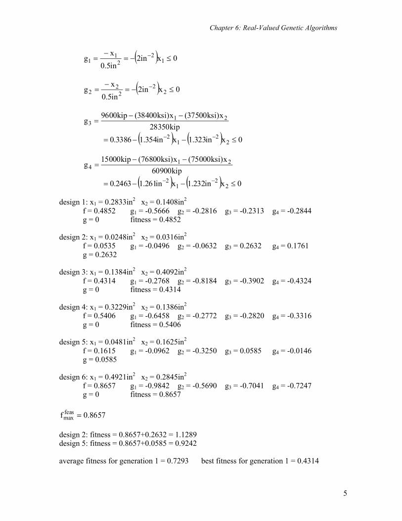
6.3.1 Example 1 The three-bar truss in Fig. 6.2 has two design variables: x1 = cross-sectional area of members AB and AD, and x2 = cross-sectional area of member AC. Suppose each design variable


4

ranges from 0.0 to 0.5 and is represented by a single continuous value gene. The starting generation consists of the following six chromosomes. 1) 0.2833, 0.1408 2) 0.0248, 0.0316 3) 0.1384, 0.4092 4) 0.3229, 0.1386 5) 0.0481, 0.1625 6) 0.4921, 0.2845 The problem is the same as in a previous example where the objective and constraints are: f = (100in)x1+(40in)x2

0xg 11 £-= 0xg 22 £-=

0x)ksi37500(x)ksi38400(kip9600g 213 £--= 0x)ksi75000(x)ksi76800(kip15000g 214 £--= Scale the objective and constraints by their respective values at x1 = x2 = 0.5in2. Then evaluate the segregation fitness of the starting generation. Calculate the average and best fitness for the generation.

Fig. 6.2 The three-bar truss

Solution Evaluating the objective and constraints at x1 = x2 = 0.5in2 gives:

f = 70in3 g1 = 0.5in2 g2 = 0.5in2 g3 = 28350kip g4 = 60900kip

The scaled objective and constraints are:

f = ( ) ( ) 221

23

21 xin571.0xin429.1in70(40in)x(100in)x -- +=

+

30 in 30 in

40 in

A

B C D

20 kip


5

( ) 0xin2in5.0xg 1

221

1 £-=-

= -

( ) 0xin2in5.0xg 2

222

2 £-=-

= -

kip28350

x)ksi37500(x)ksi38400(kip9600g 213

--=

( ) ( ) 0xin323.1xin354.13386.0 22

12 £--= --

kip60900

x)ksi75000(x)ksi76800(kip15000g 214

--=

( ) ( ) 0xin232.1xin261.12463.0 22

12 £--= --

design 1: x1 = 0.2833in2 x2 = 0.1408in2 f = 0.4852 g1 = -0.5666 g2 = -0.2816 g3 = -0.2313 g4 = -0.2844 g = 0 fitness = 0.4852 design 2: x1 = 0.0248in2 x2 = 0.0316in2 f = 0.0535 g1 = -0.0496 g2 = -0.0632 g3 = 0.2632 g4 = 0.1761 g = 0.2632 design 3: x1 = 0.1384in2 x2 = 0.4092in2 f = 0.4314 g1 = -0.2768 g2 = -0.8184 g3 = -0.3902 g4 = -0.4324 g = 0 fitness = 0.4314 design 4: x1 = 0.3229in2 x2 = 0.1386in2 f = 0.5406 g1 = -0.6458 g2 = -0.2772 g3 = -0.2820 g4 = -0.3316 g = 0 fitness = 0.5406 design 5: x1 = 0.0481in2 x2 = 0.1625in2 f = 0.1615 g1 = -0.0962 g2 = -0.3250 g3 = 0.0585 g4 = -0.0146 g = 0.0585 design 6: x1 = 0.4921in2 x2 = 0.2845in2 f = 0.8657 g1 = -0.9842 g2 = -0.5690 g3 = -0.7041 g4 = -0.7247 g = 0 fitness = 0.8657

8657.0f feasmax = design 2: fitness = 0.8657+0.2632 = 1.1289 design 5: fitness = 0.8657+0.0585 = 0.9242 average fitness for generation 1 = 0.7293 best fitness for generation 1 = 0.4314


6

6.4 Genetic Algorithms: New Generations The genetic algorithm goes through a four-step process to create a new generation from the current generation: 1) selection 2) crossover 3) mutation 4) elitism

6.4.1 Selection In this step, we select two designs from the current generation to be the mother design and the father design. Selection is based on fitness. The probability of being selected as mother or father should be greatest for those designs with the best fitness. We will mention two popular selection processes. The first selection process is known as tournament selection. With tournament selection, the user specifies a tournament size. Suppose our tournament size is three. We randomly select three designs from the current generation, and the most fit of the three becomes the mother design. Then we randomly select three more designs from the current generation, and the most fit of the three becomes the father design. One may vary the fitness pressure by changing the tournament size. The greater the tournament size, the greater the fitness pressure. In the extreme case where the tournament size is equal to the generation size, the most fit design in the current generation would always be selected as both the mother and father. At the other extreme where the tournament size is one, fitness is completely ignored in the random selection of the mother and father. The second selection process is known as roulette-wheel selection. In roulette-wheel selection, the continuous interval from zero to one is divided into subintervals, one for each design in the current generation. If we assume fitness is positive and minimized, then the lengths of the subintervals are proportional to (1/fitness)g. Thus, the longest subintervals correspond to the most fit designs in the current generation. The greater the roulette exponent, g, the greater the fitness pressure in roulette-wheel selection. A random number between zero and one is generated, and the design corresponding to the subinterval containing the random number becomes the mother design. Another random number between zero and one is generated, and the design corresponding to the subinterval containing the random number becomes the father design.

6.4.2 Crossover After selecting the mother and father designs from the current generation, two children designs are created for the next generation by the crossover process. First, we must determine whether or not crossover should occur. A crossover probability is specified by the user. A random number between zero and one is generated, and if it is less than the crossover probability, crossover is performed. Otherwise, the mother and father designs, without modification, become the two children designs. There are several different ways to perform crossover. One of the earliest crossover methods developed for genetic algorithms is single-


7

point crossover. Fig. 6.3 shows the chromosomes for a mother design and a father design. Each chromosome has n = 10 binary genes:

Fig. 6.3: Single-Point Crossover

With single-point crossover, we randomly generate an integer i from 1 to n known as the crossover point, where n is the number of genes in the chromosome. We then cut the mother and father chromosomes after gene i, and swap the tail portions of the chromosomes. In Fig. 6.3, i = 7. The first child is identical to the mother before the crossover point, and identical to the father after the crossover point. The second child is identical to the father before the crossover point, and identical to the mother after the crossover point. Another crossover method is uniform crossover. With uniform crossover, a random number r between zero and one is generated for each of the n genes. For a particular gene, if x1 is the value from the mother design and x2 is the value from the father design, then the values y1 and y2 for the children designs are:

if r £ 0.5 y1 = x2 y2 = x1 (6.4) if r > 0.5 y1 = x1 y2 = x2

The goal of crossover is to generate two new children designs that inherit many of the characteristics of the fit parent designs. However, this goal may not be achieved when the binary representation is used. Suppose the last four genes in the chromosomes in Fig. 6.3 represent a single discrete design variable whose value is equal to the base ten value of the last four genes. For the mother design, binary values of 1000 give a design variable value of 8, and for the father design, binary values of 0111 give a design variable value of 7. For the first child design, binary values of 1111 give a design variable value of 15, and for the second child, binary values of 0000 give a design variable value of 0. Thus, the parents have close values of 8 and 7, while the children have values that are very different from the parents of 15 and 0. This is known as the Hamming cliff problem of the binary representation. With a value representation, a single gene would have been used for this design variable, and

1 0 0 1 1 0 1 0 0 0

1 1 1 0 1 0 0 1 1 1

1 0 0 1 1 0 1 1 1 1

1 1 1 0 1 0 0 0 0 0

crossover point

mother

father

first child

second child


8

the parent values of 7 and 8 would have been inherited by the children with either single point or uniform crossover. Blend crossover is similar to uniform crossover since it is also performed gene by gene. Blend crossover makes it possible for children designs to receive random values anywhere in the interval between the mother value and the father value. Thus, we generate a random number between zero and one for a particular gene. If x1 is the mother value and x2 is the father value, then the children values y1 and y2 are:

y1 = (r)x1 + (1-r)x2 (6.5)

y2 = (1-r)x1 + (r)x2 It is possible to transition between uniform and blend crossover with a user-specified crossover parameter h:

y1 = (a)x1 + (1-a)x2 (6.6)

y2 = (1-a)x1 + (a)x2

where:

if r £ 0.5 2)r2(a/1 h

=

(6.7)

if r > 0.5 2)r22(1a/1 h-

-=

Note that if h = 1, then a = r and (6.6) becomes (6.5), giving blend crossover. If h = 0, then in the limit a = 0 for r £ 0.5 and a = 1 for r > 0.5, and (6.6) becomes (6.4), giving uniform crossover. In the limit as h goes to ¥ , a goes to 0.5 and (6.7) becomes y1 = y2 = (x1+x2)/2, which we may call average crossover.

6.4.3 Mutation The next step for creating the new generation is mutation. A mutation probability is specified by the user. The mutation probability is generally much lower than the crossover probability. The mutation process is performed for each gene of the first child design and for each gene of the second child design. The mutation process is very simple. One generates a random number between zero and one. If the random number is less than the mutation probability, the gene is randomly changed to another value. Otherwise, the gene is left alone. Since the mutation probability is low, the majority of genes are left alone. Mutation makes it possible to occasionally introduce diversity into the population of designs. If all possible values are equally probable for the mutated gene, the mutation is said to be uniform mutation. It may be desirable to start out with uniform mutation in the starting generation, but as one approaches the later generations one may wish to favor values near the current value of the gene. We will refer to such mutation as dynamic mutation. Let x be the


9

current value of the gene. Let r be a random number between xmin and xmax, which are the minimum and maximum possible values of x, respectively. Let the current generation number be j, and let M be the total number of generations. The parameter b is a user-supplied mutation parameter. The new value of the gene is: if r £ x a-a --+= 1

minminmin )xx()xr(xy (6.8) if r > x a-a ---= 1

maxmaxmax )xx()rx(xy where

b

÷øö

çèæ --=aM1j1 (6.9)

In Fig. 6.4, we plot the value of y as a function of r for various values of the uniformity exponent a. Note that if a = 1, then y = r, which is uniform mutation. For values of a less than one, the mutated gene value favors values near x. The bias increases as a decreases. In fact if a = 0, then y = x, which means that the gene is not mutated at all.

Fig. 6.4: Dynamic Mutation

In Fig. 6.5, we plot the uniformity exponent a versus the mutation parameter b and the generation number j. Note that if b = 0, then a = 1, and the mutation is uniform for all generations. If b > 0, then a = 1 for the starting generation (j = 1) and decreases to near zero in the final generation, giving dynamic mutation.

xmin

xmin

xmax

xmax

r x

x

y

a = 1

a = 0.5

a = 0.25

a = 0


10

Fig. 6.5: Uniformity Exponent a

6.4.4 Elitism The selection, crossover, and mutation processes produce two new children designs for the new generation. These processes are repeated again and again to create more and more children until the number of designs in the new generation reaches the specified generation size. The final step that must be performed on this new generation is elitism. This step is necessary to guarantee that the best designs survive from generation to generation. One may think of elitism as the rite of passage for children designs to qualify as future parents. The new generation is combined with the previous generation to produce a combined generation of 2N designs, where N is the generation size. The combined generation is sorted by fitness, and the N most fit designs survive as the next parent generation. Thus, children must compete with their parents to survive to the next generation.

6.4.5 Summary Note that there are many algorithm parameters in a genetic algorithm including: generation size, number of generations, penalty parameter, tournament size, roulette exponent, crossover probability, crossover parameter, mutation probability, and mutation parameter. Furthermore, there are choices between value and binary representation, penalty and segregation fitness, tournament and roulette-wheel selection, single-point, uniform, and blend crossover, and uniform and dynamic mutation. Thus, there is no single genetic algorithm that is best for all applications. One must tailor the genetic algorithm to a specific application by numerical experimentation. Genetic algorithms are far superior to random trial-and-error search. This is because they are based on the fundamental ideas of fitness pressure, inheritance, and diversity. Children designs inherit characteristics from the best designs in the preceding generation selected according to fitness pressure. Nevertheless, diversity is maintained via the randomness in the starting generation, and the randomness in the selection, crossover, and mutation processes.

1

0 M

j

1

a

b = 1

b = 1/2

b = 2

b = 0


11

Research has shown that genetic algorithms can achieve remarkable results rather quickly for problems with huge combinatorial search spaces. Unlike gradient-based algorithms, it is not possible to develop conditions of optimality for genetic algorithms. Nevertheless, for many optimization problems, genetic algorithms are the only game in town. They are tailor-made to handle discrete-valued design variables. They also work well on ground-structure problems where constraints are deleted when their associated members are deleted, since constraints need not be differentiable or continuous. Analysis program crashes can be handled in genetic algorithms by assigning poor fitness to the associated designs and continuing onward. Genetic algorithms can find all optima including the global optimum if multiple optima exist. Genetic algorithms are conceptually much simpler than gradient-based algorithms. Their only drawback is that they require many executions of the analysis program. This problem will diminish as computer speeds increase, especially since the analysis program may be executed in parallel for all designs in a particular generation.

6.4.6 Example 2 Perform selection and crossover on the starting generation from Example 1. Use tournament selection with a tournament size of two, and blend crossover according to (6.5) with a crossover probability of 0.6. Use the following random number sequence: 0.5292 0.0436 0.2949 0.0411 0.9116 0.7869 0.3775 0.8691 0.1562 0.5616 0.8135 0.4158 0.7223 0.3062 0.1357 0.5625 0.2974 0.6033 Solution

=+ ))6(5292.0(truncate1 design 4 fitness = 0.5406


mother = design 1



father = design 1

since mother and father are the same, no crossover needed

child 1 = child 2 = 0.2833, 0.1408



12


mother = design 6



father = design 3

0.1562 < 0.6 ==> perform crossover

( 5616.0 )0.4921 + (1- 5616.0 )0.1384 = 0.3370 (1- 5616.0 )0.4921 + ( 5616.0 )0.1384 = 0.2935

(0.8135) 0.2845+ (1-0.8135) 0.4092 = 0.3078 (1-0.8135) 0.2845+ (0.8135) 0.4092 = 0.3859

child 3 = 0.3370, 0.3078

child 4 = 0.2935, 0.3859



mother = design 3



father = design 1

0.5625 < 0.6 ==> perform crossover

(0.2974) 0.1384+ (1-0.2974) 0.2833= 0.2402 (1-0.2974) 0.1384+ (0.2974) 0.2833= 0.1815

(0.6033) 0.4092+ (1-0.6033) 0.1408 = 0.3027 (1-0.6033) 0.4092+ (0.6033) 0.1408 = 0.2473

child 5 = 0.2402, 0.3027

child 6 = 0.1815, 0.2473


13

6.4.7 Example 3 Perform mutation on the problem in Examples 1 and 2. Use a mutation probability of 10%, and perform dynamic mutation according to (6.8) and (6.9) with a mutation parameter of b = 5. Assume that this is the second of 10 generations. Use the following random number sequence: 0.2252 0.7413 0.5135 0.8383 0.4788 0.1916 0.4445 0.8220 0.2062 0.0403 0.5252 0.3216 0.8673 Solution

child 1, gene 1: 0.2252 > 0.1 ==> no mutation


child 1 = 0.2833, 0.1408



child 2 = 0.2833, 0.1408



child 3 = 0.3370, 0.3078



child 4 = 0.2935, 0.3859


child 5, gene 2: 0.0403 > 0.1 ==> mutate!!!

5905.0101215=÷

øö

çèæ --=a

xmin = 0.0 xmax = 0.5 x = 0.3027 (child 5, gene 2 from Example 2)

Generate random number y between xmin and xmax.


14

y = xmin + 0.5252(xmax - xmin) = 0.2626 < x

a-a --+= 1minminmin )xx()xy(xz = 0.2783

child 5 = 0.2402, 0.2783



child 6 = 0.1815, 0.2473

6.4.8 Example 4 Determine the segregation fitness for each of the 6 child chromosomes in Example 3. Then perform the elitism step to create the second generation. Calculate the average and best fitness of the second generation and compare to the average and best fitness of the starting generation. Solution Recall the formulas for the scaled objective and constraints from Example 3(?): f = ( ) ( ) 22

12 xin571.0xin429.1 -- +

( ) 0xin2g 12

1 £-= -

( ) 0xin2g 22

2 £-= -

g3 ( ) ( ) 0xin323.1xin354.13386.0 22

12 £--= --

g4 ( ) ( ) 0xin232.1xin261.12463.0 22

12 £--= --

child 1: x1 = 0.2833in2 x2 = 0.1408in2

f = 0.4852 g1 = -0.5666 g2 = -0.2816 g3 = -0.2313 g4 = -0.2844

g = 0 fitness = 0.4852

child 2: x1 = 0.2833in2 x2 = 0.1408in2

f = 0.4852 g1 = -0.5666 g2 = -0.2816 g3 = -0.2313 g4 = -0.2844

g = 0 fitness = 0.4852

child 3: x1 = 0.3370in2 x2 = 0.3078in2


15

f = 0.6573 g1 = -0.6740 g2 = -0.6156 g3 = -0.5249 g4 = -0.5579

g = 0 fitness = 0.6573

child 4: x1 = 0.2935in2 x2 = 0.3859in2

f = 0.6398 g1 = -0.5870 g2 = -0.7718 g3 = -0.5693 g4 = -0.5992

g = 0 fitness = 0.6398

child 5: x1 = 0.2402in2 x2 = 0.2783in2

f = 0.5022 g1 = -0.4804 g2 = -0.5566 g3 = -0.3548 g4 = -0.3995

g = 0 fitness = 0.5022

child 6: x1 = 0.1815in2 x2 = 0.2473in2

f = 0.4006 g1 = -0.3630 g2 = -0.4946 g3 = -0.2343 g4 = -0.2872

g = 0 fitness = 0.4006

Parent generation: design 1: 0.2833, 0.1408 fitness = 0.4852 design 2: 0.0248, 0.0316 fitness = 1.1289 design 3: 0.1384, 0.4092 fitness = 0.4314 design 4: 0.3229, 0.1386 fitness = 0.5406 design 5: 0.0481, 0.1625 fitness = 0.9242 design 6: 0.4921, 0.2845 fitness = 0.8657

Child generation:

child 1: 0.2833, 0.1408 fitness = 0.4852 child 2: 0.2833, 0.1408 fitness = 0.4852 child 3: 0.3370, 0.3078 fitness = 0.6573 child 4: 0.2935, 0.3859 fitness = 0.6398 child 5: 0.2402, 0.2783 fitness = 0.5022 child 6: 0.1815, 0.2473 fitness = 0.4006

Generation 2:

design 1: 0.1815, 0.2473 fitness = 0.4006 design 2: 0.1384, 0.4092 fitness = 0.4314 design 3: 0.2833, 0.1408 fitness = 0.4852 design 4: 0.2833, 0.1408 fitness = 0.4852 design 5: 0.2833, 0.1408 fitness = 0.4852 design 6: 0.2402, 0.2783 fitness = 0.5022

average fitness for generation 2 = 0.4650 best fitness for generation 2 = 0.4006 This is significantly better than the starting generation.


16

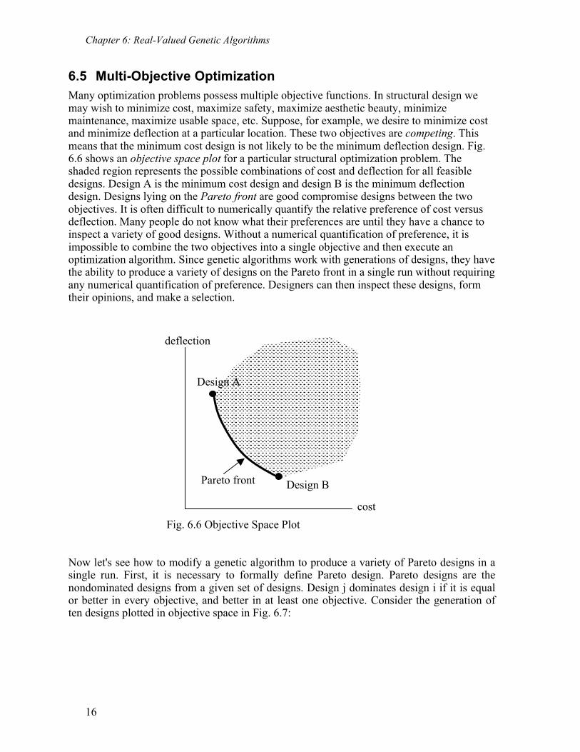
6.5 Multi-Objective Optimization Many optimization problems possess multiple objective functions. In structural design we may wish to minimize cost, maximize safety, maximize aesthetic beauty, minimize maintenance, maximize usable space, etc. Suppose, for example, we desire to minimize cost and minimize deflection at a particular location. These two objectives are competing. This means that the minimum cost design is not likely to be the minimum deflection design. Fig. 6.6 shows an objective space plot for a particular structural optimization problem. The shaded region represents the possible combinations of cost and deflection for all feasible designs. Design A is the minimum cost design and design B is the minimum deflection design. Designs lying on the Pareto front are good compromise designs between the two objectives. It is often difficult to numerically quantify the relative preference of cost versus deflection. Many people do not know what their preferences are until they have a chance to inspect a variety of good designs. Without a numerical quantification of preference, it is impossible to combine the two objectives into a single objective and then execute an optimization algorithm. Since genetic algorithms work with generations of designs, they have the ability to produce a variety of designs on the Pareto front in a single run without requiring any numerical quantification of preference. Designers can then inspect these designs, form their opinions, and make a selection.

Fig. 6.6 Objective Space Plot

Now let's see how to modify a genetic algorithm to produce a variety of Pareto designs in a single run. First, it is necessary to formally define Pareto design. Pareto designs are the nondominated designs from a given set of designs. Design j dominates design i if it is equal or better in every objective, and better in at least one objective. Consider the generation of ten designs plotted in objective space in Fig. 6.7:

Design A

Design B

deflection

cost

Pareto front


17

Fig. 6.7: A Generation of Ten Designs

Design H dominates design D because it has lower values in both objectives. Design B dominates design D because it has a lower value of cost and an equal value of deflection. There are no designs that dominate designs A, B, H, of J. These four designs are the Pareto designs for this particular set of ten designs. It is our goal that the genetic algorithm converges to the Pareto designs for the set of all possible designs. We do this by modifying the fitness function. We will examine three different fitness functions for multi-objective optimization. The first fitness function is called the scoring fitness function. For a particular design i in a particular generation, the scoring fitness is equal to one plus the number of designs that dominate design i. We minimize this fitness function. For example, in Fig. 6.7, the scoring fitness of design D is 3 since it is dominated by designs B and H. The scoring fitness of design F is 10 since it is dominated by all other designs. Note that the scoring fitness of the Pareto designs is one since they are nondominated. Another fitness function for multi-objective optimization is the ranking fitness function. This fitness function is also minimized. To begin, the Pareto designs in the generation are identified and assigned a rank of one. Thus, designs A, B, H, and J in Fig. 6.7 are assigned a rank of one. These designs are temporarily deleted, and the Pareto designs of the remaining set are identified and assigned a rank of two. Thus, designs C, D, and I in Fig. 6.7 are assigned a rank of two. These designs are temporarily deleted, and the Pareto designs of the remaining set are identified and assigned a rank of three. Thus, designs E and G in Fig. 6.7 are assigned a rank of three. This procedure continues until all designs in the generation have been assigned a rank. Thus, design F in Fig. 6.7 is assigned a rank of four. The ranking fitness differs from the scoring fitness. In Fig. 6.7, designs C and D have the same rank but they have different scores (design C has a score of 2 and design D has a score of 3).

A

deflection

cost

B

C

D

E F

G

I H

J


18

Note that since all Pareto designs in a particular generation have ranks and scores of one, they are all regarded as equally fit. Thus, there is nothing to prevent clustering on the Pareto front. Indeed, numerical experiments have shown that genetic algorithms with scoring or ranking fitness will often converge to a single design on the Pareto front. We also observe that the scoring and ranking fitness functions are discontinuous functions of the objective values. An infinitesimal change in the value of an objective may cause the ranking or scoring fitness to jump to another integer value. The third multi-objective fitness function we will consider is the maximin fitness function. We derive this fitness function directly from the definition of dominance. Let us assume that the designs in a particular generation are distinct in objective space, and that the n objectives are minimized. Let j

kf value= of the k’th objective for design i. Design j dominates design i if:

i jk kf f³ for 1 tok n= (6.10)

Equation (6.10) is equivalent to:

min( ) 0i jk kkf f- ³ (6.11)

Thus, design i is a dominated design if:

( )max min( ) 0i jk kkj if f

¹- ³

(6.12) The maximin fitness of design i is:

( )max min( ) 0i jk kkj if f

¹- ³ (6.13)

The maximin fitness is minimized. The maximin fitness of Pareto designs will be less than zero, while the maximin fitness of dominated designs will be greater than or equal to zero. The maximin fitness of all Pareto designs is not the same. The more isolated a design is on the Pareto front, the more negative its maximin fitness will be. On the other hand, two designs that are infinitesimally close to each other on the Pareto front will have maximin fitnesses that are negative and near zero. Thus, the maximin fitness function avoids clustering. Furthermore, the maximin fitness is a continuous function of the objective values.

6.5.1 Example 5 Consider an optimization problem with two design variables, x1 and x2, no constraints, and two objectives:

211 xx10f -= 1

22 x

x1f

+=

A particular generation in a genetic algorithm consists of the following six designs:


19

design 1 x1=1 x2=1 design 4 x1=1 x2=0



Calculate the objective values for these designs and make an objective space plot of this generation. Solution

91)1(10f11 =-= 2111f 12 =

+=

28)1(10f 21 =-= 9181f 22 =

+=

1555)7(10f 31 =-= 87551f 32 =

+=

100)1(10f 41 =-= 1101f 42 =

+=

1317)3(10f 51 =-= 63171f 52 =

+=

911)2(10f 61 =-= 62111f 62 =

+=

Fig. 6.8

6.5.2 Example 6 Determine the scoring fitness and ranking fitness for the designs in Example 5.

f1

f2

1

2 3

4

5 6


20

Solution

Scoring Fitness:

Designs 2, 1, and 4 are not dominated by any other designs. Their score is 1.

Design 6 is dominated by design 1. Its score is 2.

Design 5 is dominated by designs 1, 4, and 6. Its score is 4.

Design 3 is dominated by designs 1, 4, 6, and 5. Its score is 5.

Ranking Fitness:

Designs 2, 1, and 4 have a rank of 1.

Design 6 has a rank of 2.



6.5.3 Example 7 Determine the maximin fitness for the designs in Example 5.

Solution

design 1: ( ) ( ) ( )( ) ( ) ÷÷

ø

öççè

æ----

------62 ,99min,62 ,139min

,12 ,109min,82 ,159min,92 ,29minmax

( ) ( ) ( ) ( ) ( )( )4,0min,4,4min,1,1min,6,6min,7,7minmax -------=

( )4,4,1,6,7max -----=

1-=

design 2: ( ) ( ) ( )( ) ( ) ÷÷

ø

öççè

æ----

------69 ,92min,69 ,132min

,19 ,102min,89 ,152min,29 ,92minmax

( ) ( ) ( ) ( ) ( )( )3,7min,3,11min,8,8min,1,13min,7,7minmax -----=

( )7,11,8,13,7max -----=

7-=


21

design 3: ( ) ( ) ( )( ) ( ) ÷÷

ø

öççè

æ----

------68 ,915min,68 ,1315min

,18 ,1015min,98 ,215min,28 ,915minmax

( ) ( ) ( ) ( ) ( )( )2,6min,2,2min,7,5min,1,13min,6,6minmax -=

( )2,2,5,1,6max -=

6=

design 4: ( ) ( ) ( )( ) ( ) ÷÷

ø

öççè

æ----

------61 ,910min,61 ,1310min

,81 ,1510min,91 ,210min,21 ,910minmax

( ) ( ) ( ) ( ) ( )( )5,1min,5,3min,7,5min,8,8min,1,1minmax -------=

( )5,5,7,8,1max -----=

1-=

design 5: ( ) ( ) ( )( ) ( ) ÷÷

ø

öççè

æ----

------66 ,913min,16 ,1013min

,86 ,1513min,96 ,213min,26 ,913minmax

( ) ( ) ( ) ( ) ( )( )0,4min,5,3min,2,2min,3,11min,4,4minmax ---=

( )0,3,2,3,4max --=

4=

design 6: ( ) ( ) ( )( ) ( ) ÷÷

ø

öççè

æ----

------66 ,139min,16 ,109min

,86 ,159min,96 ,29min,26 ,99minmax

( ) ( ) ( ) ( ) ( )( )0,4min,5,1min,2,6min,3,7min,4,0minmax -----=

( )4,1,6,3,0max ----=

0=

Note that design 2 is more fit than designs 1 and 4 even though all three are Pareto designs

(negative fitness). This is because designs 1 and 4 are clustered.

real-valued genetic algorithms 6.1 introductionevolutionary algorithms mimic the optimization...

Documents