real-time road traffic fusion and prediction with gps and
TRANSCRIPT
Real-Time Road Traffic Fusion and Predictionwith GPS and Fixed-Sensor Data
Wei Shen@WalmartLabs, Walmart eCommerce
San Bruno, CA 94066 USAEmail: [email protected]
Laura WynterIBM Watson Research Center
Yorktown Heights, NY 10598 USAEmail: [email protected]
Abstract—GPS devices offer new opportunities forshort-term traffic prediction, especially in arterial roadnetworks where traditional fixed-location sensors aresparse or unavailable. However, GPS data is often sparseboth temporally and spatially. On its own, it is ofteninsufficient for real-time traffic prediction. Hence, weconsider the fusion of two types of data for the purposeof real-time traffic fusion and prediction: GPS data thatis provided as point speeds, rather than trajectories, aswell as (non real-time) traffic data such as is availablefrom fixed sensors.
I. INTRODUCTION
Real-time road traffic data fusion is an importantcomponent of modern traffic management and infor-mation systems. Reliable prediction of near-term trafficconditions in road networks allows traffic managementagencies to generate proactive traffic operation strate-gies to alleviate congestion and allows both publicagencies and private companies to provide accuratetravel time estimates to road users.
In the past two decades, much research effort hasbeen invested in developing accurate and robust trafficprediction models. The modeling approaches can beclassified into parametric methods and non-parametricmethods. The former category relies primarily onstatistical techniques, including historical average andsmoothing techniques [1], [2], autoregressive movingaverage models [3]–[8], and Kalman filter algorithms[9], [10]. The main non-parametric approaches pub-lished to date include non-parametric regression [11]–[13] and artificial neural networks (ANN) [14]–[19].See [20] for a somewhat dated review of differenttraffic prediction models.
The above approaches have been designed in gen-eral for traffic prediction based on fixed-location datasources such as inductive loops, roadside radar sensors,and traffic cameras. When using fixed-location sensordata only, taking into account spatial and temporalcorrelations of traffic flow can be done in a straight-forward manner. For example, traffic measurements on
neighboring links can be used to formulate a univariateor mutlivariate linear/nonlinear prediction model.
While fixed-location traffic sensors are commonlyavailable on expressways and other major roadways,real-time traffic data using fixed-location sensors is farless ubiquitous on urban networks. The proliferationof GPS devices in fleets of vehicles, passenger cars inthe form of in-vehicle navigation systems, and morerecently from applications on smart phones, has ledto an increasing emphasis on using GPS data for theidentification of traffic speeds on the roads. Someproducts exist in the marketplace to determine traffic“color maps” for GPS-enabled mobile phones equippedwith dedicated applications that transmit periodicallylocations to a server. Such traffic estimation is relatedto the traffic prediction problem that we are interestedin but is different in two important ways. On the onehand, we are interested in quantitative traffic predictionthat produces a set of future speeds on the variousroad links, rather than the types of ranges producedfor use on “color maps”. Secondly, we are interestedin going beyond real-time traffic estimation to futuretraffic prediction, which in general requires more datathan the real-time estimation problem.
There are two major issues in using GPS data fortraffic prediction. First, disclosing detailed vehiculartrajectory data is always associated with privacy andsecurity concerns. Even if trajectory data is broad-casted in an anonymous manner, it is still possibleto identify individuals from the trajectory data [21].Hence, in some cases, GPS measurements are sampledat random times/locations/devices so that vehiculartrajectories cannot be inferred. One example of suchan approach is the Virtual Trip Line proposed by [22],which is essentially a spatial trigger for GPS devicesto collect and report measurements when pre-definedvirtual lines in the network are crossed. The datacollection procedure for our study is similar in natureto the idea of Virtual Trip Line. The only difference isthat sampling is performed on devices rather than on
1468
locations. More specifically, for each given interval,only a sampled collection of GPS devices report theirlocation and speed information. The second challengeis that traditional traffic prediction methods which arebased on reliable traffic observations from fixed loca-tions are usually inapplicable in this context. Indeed,the proportion of vehicles who disclose their locationor speed information to any given application provideris typically very low and hence the amount of real-timeand historical data on each road link is insufficient forstandard traffic prediction approaches to apply.
The method presented in this paper is based onthe approach developed for such a problem as partof the 2010 IEEE International Conference on DataMining (ICDM) TomTom Traffic Prediction Contestfor Intelligent GPS Navigation. The authors were partof the team which placed second worldwide in thatcontest. The remainder of this paper is structured asfollows. Section 2 introduces the problem setting andthe data used for developing our approach. Section3 describes the hybrid method developed. Section 4presents the prediction performance of the proposedmethod on the test data set, and Section 5 concludesthe paper by summarizing the major findings.
II. PROBLEM SETTING AND DATA
The traffic prediction problem investigated in thispaper is as follows: Suppose that GPS data is availablefrom a sampling of drivers at random points on a roadnetwork. Suppose further that trajectory data cannotbe gathered, as is the case with numerous smartphoneapplications that sample user locations and speeds atseparate points in time far enough apart to be unableto redraw the users’ paths. This is done primarily toprotect the users’ privacy as part of an opt-in approachto the application. Since the data is available onlyto the particular application provider, the subset ofthe population available to the provider is limited. Inaddition, given the sampling that the provider agreesto do to protect users’ privacy, the available populationis reduced further still.
Because of the sparsity of available signals on all ofthe urban road links at all points in time, a secondarysource of data is useful. Specifically, we make use of aset of additional information on average travel speedsfor the links of interest, which may have been obtainedfrom other sources but not available as a fixed-sensor-based real-time data feed. We term this data source as“historical” because in our setting they are availablefor the training data but not as part of the testing dataset. Below is just one out of many examples of such a“historical” data source. The GPS device/smart phoneservice provider sends out probe vehicles or removable
speed sensors to measure the actual space-mean speedon the critical links periodically (say one week perquarter) for validation and calibration purpose. To saveresource, such measuring procedure can rotate over thelinks of interests and do not need to be performedsimultaneously.
The goal, as stated previously, is to perform near-term prediction of traffic speeds on selected road links.
The specific data used in this paper was obtainedas part of the 2010 IEEE ICDM Traffic Predictioncompetition. In this case, the GPS data was generatedby a traffic simulation program rather than from liveusers. The simulator, called the Traffic SimulationFramework (TSF), was developed at the Universityof Warsaw, and is based on the well-known Nagel-Schreckenberg’s cellular automata traffic flow models[23]. The functionality of TSF was described in detailin [24].
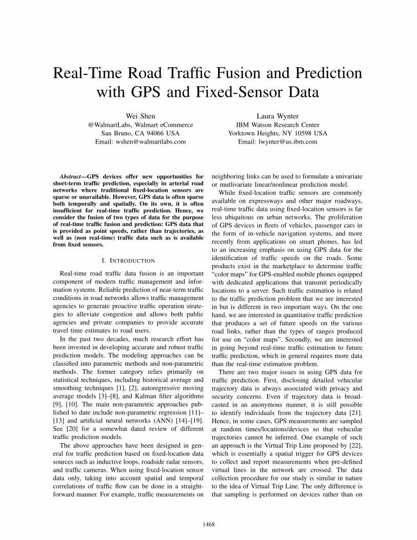
Traffic simulation was performed for the networkof Warsaw, Poland (Figure 1), and contains in all18716 nodes and 35170 links. Among the links, 8631are classified as major roads, and 100 are furthertermed “critical” links. Our goal was to perform trafficprediction on the 100 critical links.
Critical road segments
Major Road
Minor road
Fig. 1. Network of Warsaw, Poland.
The simulation was run for essentially 500simulation-hours, thereby representing 50 10-hour day-time periods on similar days, such as 10 weeks’ worthof five-day weeks, during the daytime hours. Thatdata was considered to be historical data to be usedfor training. An additional set of data of the samequantity was generated and was used as testing data.However, for each hour of the testing data set, onlyGPS information of the first 30 minutes of each of the500 hours was revealed. In terms of simulated sampledGPS data, 1% of the vehicles simulated were sampledduring each 10-second interval and the instantaneousspeed and location recorded.
1469
Each GPS record contains a timestamp, latitude andlongitude, and the instantaneous speed of the sampledvehicle. Before any prediction model can be applied, aprocedure is needed to map GPS location to the roadsegments on the network. Since GPS data are generallynoisy, the reported coordinates may not necessarily fallprecisely on any link. Map-matching algorithms [25],[26] are therefore needed to accurately approximatethe location of the GPS points on the links. Since thesimulated traffic data was less noisy, we were able toemploy the built-in spatial join function in ArcGIS forthe map matching function; specifically, each GPS datapoint was associated with the closest link within a 20-meter radius. If no such link is found, the GPS datapoint was discarded. To reduce computational time,only major links were included as candidate links formatching. The map-matching procedure was performedfor the GPS data points of both the training and testdata sets. Roughly 80% of the GPS points were ableto be map-matched of the approximately 280,000 GPSpoints provided during an average training hour.
As the secondary source of average-case data, 6-minute (harmonic) average speeds were provided forall of the 100 critical links for each hour of the trainingdata. No average-case speed information was availablefor the testing data to reflect the fact that such datais not typically available on the links in question as areal-time feed.
As part of the IEEE ICDM competition, the ob-jective was to perform two traffic speed predictionson the full set of 100 critical links: a 6-minute-aheadprediction and a 30-minute-ahead prediction, in bothcases with the speeds being harmonic averages of thepreceding 6 minutes.
Suppose the speed estimate for a link during any6-min interval is regarded as missing only if no GPSsample points fall on the link during the correspondingtime interval. In the training data, the overall missingdata percentage is 76.94% on the major links and68.24% on the 100 critical links. In fact, 22 of the100 critical links have no GPS records at all in any ofthe training data history.
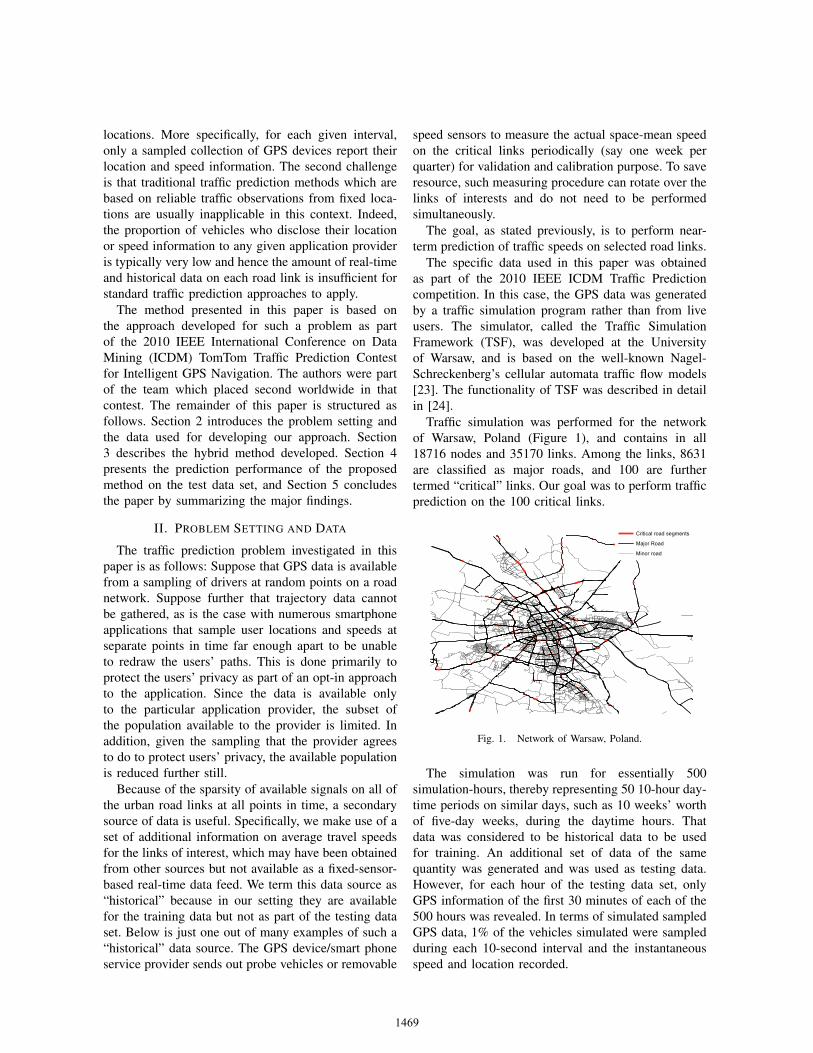
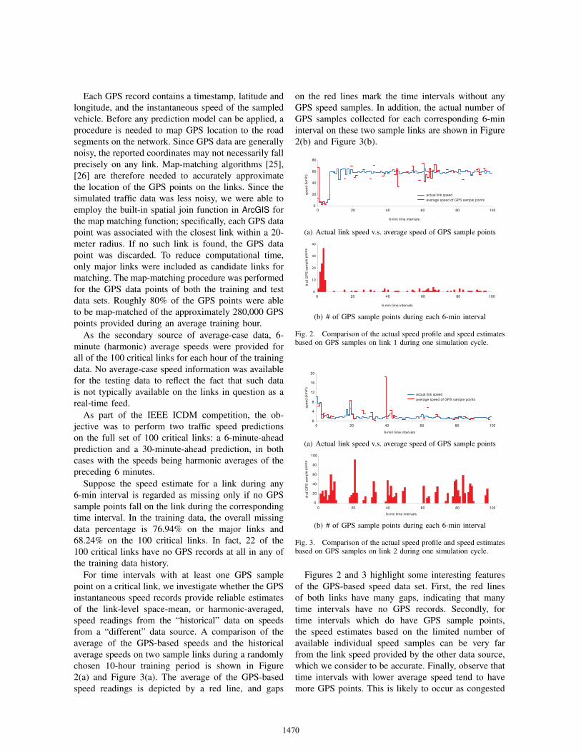
For time intervals with at least one GPS samplepoint on a critical link, we investigate whether the GPSinstantaneous speed records provide reliable estimatesof the link-level space-mean, or harmonic-averaged,speed readings from the “historical” data on speedsfrom a “different” data source. A comparison of theaverage of the GPS-based speeds and the historicalaverage speeds on two sample links during a randomlychosen 10-hour training period is shown in Figure2(a) and Figure 3(a). The average of the GPS-basedspeed readings is depicted by a red line, and gaps
on the red lines mark the time intervals without anyGPS speed samples. In addition, the actual number ofGPS samples collected for each corresponding 6-mininterval on these two sample links are shown in Figure2(b) and Figure 3(b).
0
20
40
60
80
0 20 40 60 80 100
6-min time intervals
sp
ee
d (
km
/h)
actual link speed
average speed of GPS sample points
(a) Actual link speed v.s. average speed of GPS sample points
0
10
20
30
40
0 20 40 60 80 100
6-min time intervals#
of G
PS
sa
mp
le p
oin
ts
(b) # of GPS sample points during each 6-min interval
Fig. 2. Comparison of the actual speed profile and speed estimatesbased on GPS samples on link 1 during one simulation cycle.
0
4
8
12
16
20
0 20 40 60 80 100
actual link speed
average speed of GPS sample points
sp
ee
d (
km
/h)
6-min time intervals
(a) Actual link speed v.s. average speed of GPS sample points
0
20
40
60
80
100
0 20 40 60 80 100
# o
f G
PS
sa
mp
le p
oin
ts
6-min time intervals
(b) # of GPS sample points during each 6-min interval
Fig. 3. Comparison of the actual speed profile and speed estimatesbased on GPS samples on link 2 during one simulation cycle.
Figures 2 and 3 highlight some interesting featuresof the GPS-based speed data set. First, the red linesof both links have many gaps, indicating that manytime intervals have no GPS records. Secondly, fortime intervals which do have GPS sample points,the speed estimates based on the limited number ofavailable individual speed samples can be very farfrom the link speed provided by the other data source,which we consider to be accurate. Finally, observe thattime intervals with lower average speed tend to havemore GPS points. This is likely to occur as congested
1470
links usually accommodate more vehicles at any pointin time, and hence are likely to contain more GPSsamples.
III. METHODOLOGY
A straightforward approach for traffic predictionbased on GPS data is to construct good estimates oflink speed for each time interval on each link, based onits corresponding GPS speed samples, and treat them asfixed location observations. Then any number of trafficprediction approaches could be used on the aggregateddata.
The question is whether this method is feasible withsuch a low sampling rate (i.e., 1%). Figures 2 and 3imply that such a method will not fare well due to theunreliable nature of the sampled GPS speed data. Assuch, averaging the values does not tend to replicateobserved speeds from other data sources.
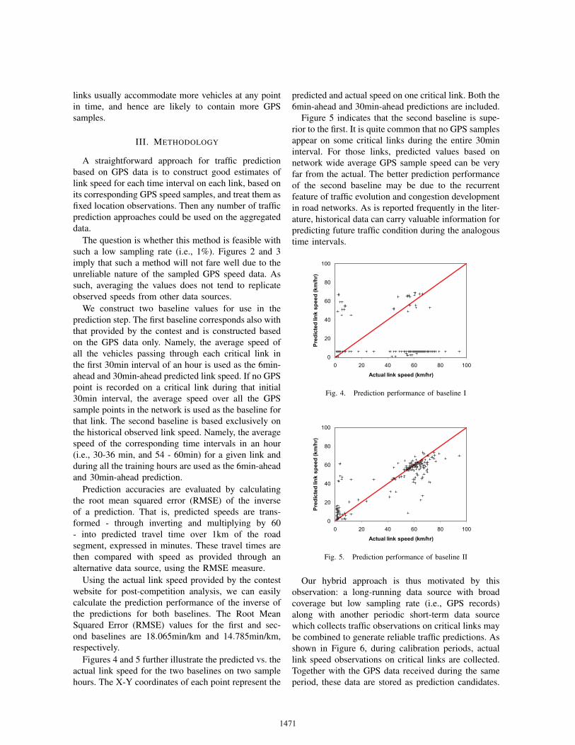
We construct two baseline values for use in theprediction step. The first baseline corresponds also withthat provided by the contest and is constructed basedon the GPS data only. Namely, the average speed ofall the vehicles passing through each critical link inthe first 30min interval of an hour is used as the 6min-ahead and 30min-ahead predicted link speed. If no GPSpoint is recorded on a critical link during that initial30min interval, the average speed over all the GPSsample points in the network is used as the baseline forthat link. The second baseline is based exclusively onthe historical observed link speed. Namely, the averagespeed of the corresponding time intervals in an hour(i.e., 30-36 min, and 54 - 60min) for a given link andduring all the training hours are used as the 6min-aheadand 30min-ahead prediction.
Prediction accuracies are evaluated by calculatingthe root mean squared error (RMSE) of the inverseof a prediction. That is, predicted speeds are trans-formed - through inverting and multiplying by 60- into predicted travel time over 1km of the roadsegment, expressed in minutes. These travel times arethen compared with speed as provided through analternative data source, using the RMSE measure.
Using the actual link speed provided by the contestwebsite for post-competition analysis, we can easilycalculate the prediction performance of the inverse ofthe predictions for both baselines. The Root MeanSquared Error (RMSE) values for the first and sec-ond baselines are 18.065min/km and 14.785min/km,respectively.
Figures 4 and 5 further illustrate the predicted vs. theactual link speed for the two baselines on two samplehours. The X-Y coordinates of each point represent the
predicted and actual speed on one critical link. Both the6min-ahead and 30min-ahead predictions are included.
Figure 5 indicates that the second baseline is supe-rior to the first. It is quite common that no GPS samplesappear on some critical links during the entire 30mininterval. For those links, predicted values based onnetwork wide average GPS sample speed can be veryfar from the actual. The better prediction performanceof the second baseline may be due to the recurrentfeature of traffic evolution and congestion developmentin road networks. As is reported frequently in the liter-ature, historical data can carry valuable information forpredicting future traffic condition during the analogoustime intervals.
0
20
40
60
80
100
0 20 40 60 80 100
Pre
dic
ted
lin
k s
pe
ed
(k
m/h
r)
Actual link speed (km/hr)
Fig. 4. Prediction performance of baseline I
0
20
40
60
80
100
0 20 40 60 80 100
Pre
dic
ted
lin
k s
pe
ed
(k
m/h
r)
Actual link speed (km/hr)
Fig. 5. Prediction performance of baseline II
Our hybrid approach is thus motivated by thisobservation: a long-running data source with broadcoverage but low sampling rate (i.e., GPS records)along with another periodic short-term data sourcewhich collects traffic observations on critical links maybe combined to generate reliable traffic predictions. Asshown in Figure 6, during calibration periods, actuallink speed observations on critical links are collected.Together with the GPS data received during the sameperiod, these data are stored as prediction candidates.
1471
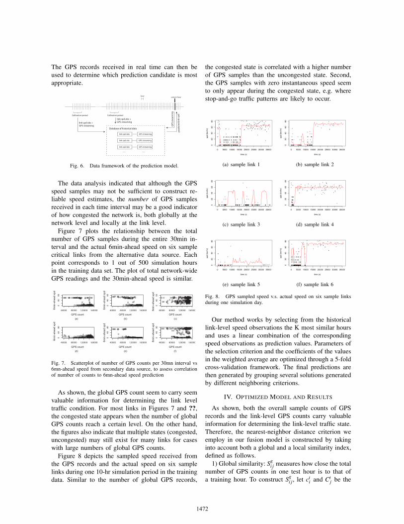
The GPS records received in real time can then beused to determine which prediction candidate is mostappropriate.
hourcurrent hour
Database of historical data
Calibration period
Calibration period
GP
S s
tre
am
ing
pre
dic
ted
lin
k s
pd
link spd obs +
GPS streaming
link spd obs +
GPS streaming
link spd obs GPS streaming
link spd obs GPS streaming
link spd obs GPS streaming
...... ......
Fig. 6. Data framework of the prediction model.
The data analysis indicated that although the GPSspeed samples may not be sufficient to construct re-liable speed estimates, the number of GPS samplesreceived in each time interval may be a good indicatorof how congested the network is, both globally at thenetwork level and locally at the link level.
Figure 7 plots the relationship between the totalnumber of GPS samples during the entire 30min in-terval and the actual 6min-ahead speed on six samplecritical links from the alternative data source. Eachpoint corresponds to 1 out of 500 simulation hoursin the training data set. The plot of total network-wideGPS readings and the 30min-ahead speed is similar.
40000 80000 120000 160000
040
80
40000 80000 120000 160000
040
80
40000 80000 120000 160000
040
80
40000 80000 120000 160000
040
80
40000 80000 120000 160000
040
80
40000 80000 120000 160000
040
80
GPS count GPS count GPS count
6m
in-a
he
ad
sp
d
6m
in-a
he
ad
sp
d
6m
in-a
he
ad
sp
d
(a) (b) (c)
GPS count GPS count GPS count
(d) (e) (f)
6m
in-a
he
ad
sp
d
6m
in-a
he
ad
sp
d
6m
in-a
he
ad
sp
d
Fig. 7. Scatterplot of number of GPS counts per 30mn interval vs6mn-ahead speed from secondary data source, to assess correlationof number of counts to 6mn-ahead speed prediction
As shown, the global GPS count seem to carry seemvaluable information for determining the link leveltraffic condition. For most links in Figures 7 and ??,the congested state appears when the number of globalGPS counts reach a certain level. On the other hand,the figures also indicate that multiple states (congested,uncongested) may still exist for many links for caseswith large numbers of global GPS counts.
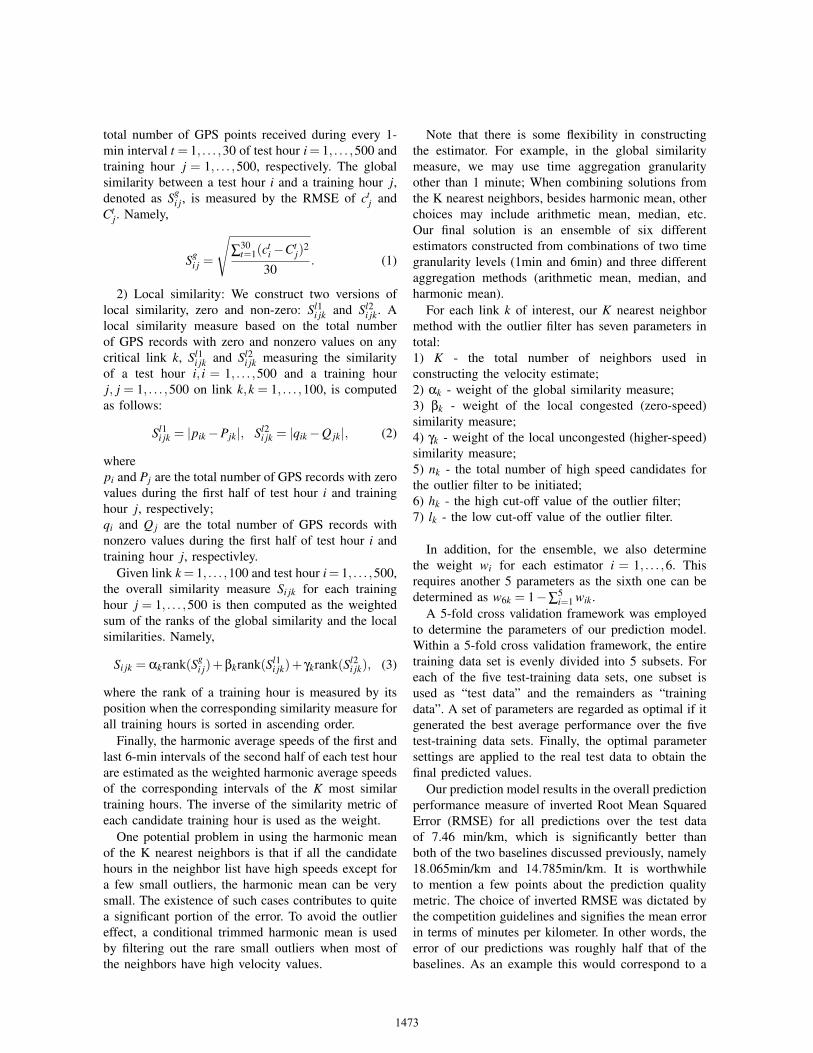
Figure 8 depicts the sampled speed received fromthe GPS records and the actual speed on six samplelinks during one 10-hr simulation period in the trainingdata. Similar to the number of global GPS records,
the congested state is correlated with a higher numberof GPS samples than the uncongested state. Second,the GPS samples with zero instantaneous speed seemto only appear during the congested state, e.g. wherestop-and-go traffic patterns are likely to occur.
0 5000 10000 15000 20000 25000 30000 35000
020
40
60
80
time (s)
sp
d (
km
/hr) *
*
*
*
*
*
*
*
*
*
**
*****
*
******
**
*********
*
*
*
********
*
*
*
*******
*
*
*
**************
*
*
*
***************
*
**
************************
*
*
*************
*
**********
**
*****
*
******************
*
********
*
****
*
****************
*
*
*
*
*******
*
**
**
**
******
**
*
******
*
**
*
*
***********************
*
*
*
*
****
*
*
*
***
**
*
**********
*
*
*******
*
****
**
********
*
*
********
*
****
**
*******
*
*******
*
** ******
**
*******
**
*********
*
****
*
******
***
*******
*
*******
*
*******
*
******
*
**
**
***
*
*
*
***********
*
**
*
**
**
*
*
**************
*
***********************
*
*
*
*******
*
*
*******
*
*****
**
*******************
*
*******
*
***
*
*****
***
*
*
****
*
********
*
*
*
**
********
*
*
*
*
*******
**
***
*
*
*******
*
*****
**
*****
***
**********
*
**
*******
*
**
*
******
***
*
*
*
*******
*
********
*
**
*
**
*
******
*
*
*
*******
*
*
*
**
*
***
*
**
**
*
***
*
* * *
**
*
*
***
*
*
*
**
*
**
****
***
*
*
****
**
*
*
**
*
*
***
**
*
*
*
*
*
*
***
*
*
*
*
*
***
**
*
****
**
*
*
***
*
**
*
**
(a) sample link 1
0 5000 10000 15000 20000 25000 30000 35000
020
40
60
80
time (s)
sp
d (
km
/hr)
**********
*
*
*
******
**
*
*******
*
*********************************
*
****** ********
*
***************** *******
*
*********************************
*
******
*
*
***********
*
*
*
**************
*
***
***
*
*******
*
*
*********************
*
********
*
********
*
*
********
*
**
*
*************
****
**************
*
*********
*
*******
**
*
*
**
*
***
(b) sample link 2
0 5000 10000 15000 20000 25000 30000 350000
20
40
60
80
time (s)
spd (
km
/hr)
********** ********
*
*
*********
*
***********************
*
******** *************** ********
*
** *****************
*
*** *****************
*
************
*
*******
*
*******
*
*******************************
*
************ ******
*
********** *************** **************** *** ****** ****
(c) sample link 3
0 5000 10000 15000 20000 25000 30000 35000
020
40
60
80
time (s)
spd (
km
/hr) *
**
**
*
******
*
**********
**
*
**
*******************
*
*
*
*
**
*
*
**********************
***
*
*
*
********
*
*
*
*
**
**
**
*
**
*
* ***
*
*
***
*
*
**
*
*
*
*
*
**
*
*
*
**
***
*** ***
*
*
*
*
**
*
*
*
***
*
**
(d) sample link 4
0 5000 10000 15000 20000 25000 30000 35000
020
40
60
80
time (s)
spd (
km
/hr)
*
********
*
**
*
************************
*
*************** **************** *
*
********
*
***************
*
***
*
* **
(e) sample link 5
0 5000 10000 15000 20000 25000 30000 35000
020
40
60
80
time (s)
spd (
km
/hr)
*
**
**
**
*********
*
**
*
***
******
*
*
*
***
*
* *
*
******
*
********
*
**********************
*
*********
*
**************************
*
***********
**
*
*
*********************
*
********
*
**
**
*******
*
**************
*
*
*
*
*
*
**********
*
**
*
**
*********
*
**************
*
***********************
**
*
*
*
************
*
***
*
*
*
*
**********
*
*
*
************
*
*
****
*
***************
**
**********************
*
*
******************
*
**
*
*
*
**********
*
***************
*
*******
*
*******
*
*
*
***
***
**************
*
*
********
*
*
*
**
*
*
* **
*
* *
*** **
*
**
*
*
**
* *
*
**
(f) sample link 6
Fig. 8. GPS sampled speed v.s. actual speed on six sample linksduring one simulation day.
Our method works by selecting from the historicallink-level speed observations the K most similar hoursand uses a linear combination of the correspondingspeed observations as prediction values. Parameters ofthe selection criterion and the coefficients of the valuesin the weighted average are optimized through a 5-foldcross-validation framework. The final predictions arethen generated by grouping several solutions generatedby different neighboring criterions.
IV. OPTIMIZED MODEL AND RESULTS
As shown, both the overall sample counts of GPSrecords and the link-level GPS counts carry valuableinformation for determining the link-level traffic state.Therefore, the nearest-neighbor distance criterion weemploy in our fusion model is constructed by takinginto account both a global and a local similarity index,defined as follows.
1) Global similarity: Sgi j measures how close the total
number of GPS counts in one test hour is to that ofa training hour. To construct Sg
i j, let cti and Ct
j be the
1472
total number of GPS points received during every 1-min interval t = 1, . . . ,30 of test hour i = 1, . . . ,500 andtraining hour j = 1, . . . ,500, respectively. The globalsimilarity between a test hour i and a training hour j,denoted as Sg
i j, is measured by the RMSE of ctj and
Ctj. Namely,
Sgi j =
√∑
30t=1(c
ti−Ct
j)2
30. (1)
2) Local similarity: We construct two versions oflocal similarity, zero and non-zero: Sl1
i jk and Sl2i jk. A
local similarity measure based on the total numberof GPS records with zero and nonzero values on anycritical link k, Sl1
i jk and Sl2i jk measuring the similarity
of a test hour i, i = 1, . . . ,500 and a training hourj, j = 1, . . . ,500 on link k,k = 1, . . . ,100, is computedas follows:
Sl1i jk = |pik−Pjk|, Sl2
i jk = |qik−Q jk|, (2)
wherepi and Pj are the total number of GPS records with zerovalues during the first half of test hour i and traininghour j, respectively;qi and Q j are the total number of GPS records withnonzero values during the first half of test hour i andtraining hour j, respectivley.
Given link k = 1, . . . ,100 and test hour i = 1, . . . ,500,the overall similarity measure Si jk for each traininghour j = 1, . . . ,500 is then computed as the weightedsum of the ranks of the global similarity and the localsimilarities. Namely,
Si jk = αkrank(Sgi j)+βkrank(Sl1
i jk)+ γkrank(Sl2i jk), (3)
where the rank of a training hour is measured by itsposition when the corresponding similarity measure forall training hours is sorted in ascending order.
Finally, the harmonic average speeds of the first andlast 6-min intervals of the second half of each test hourare estimated as the weighted harmonic average speedsof the corresponding intervals of the K most similartraining hours. The inverse of the similarity metric ofeach candidate training hour is used as the weight.
One potential problem in using the harmonic meanof the K nearest neighbors is that if all the candidatehours in the neighbor list have high speeds except fora few small outliers, the harmonic mean can be verysmall. The existence of such cases contributes to quitea significant portion of the error. To avoid the outliereffect, a conditional trimmed harmonic mean is usedby filtering out the rare small outliers when most ofthe neighbors have high velocity values.
Note that there is some flexibility in constructingthe estimator. For example, in the global similaritymeasure, we may use time aggregation granularityother than 1 minute; When combining solutions fromthe K nearest neighbors, besides harmonic mean, otherchoices may include arithmetic mean, median, etc.Our final solution is an ensemble of six differentestimators constructed from combinations of two timegranularity levels (1min and 6min) and three differentaggregation methods (arithmetic mean, median, andharmonic mean).
For each link k of interest, our K nearest neighbormethod with the outlier filter has seven parameters intotal:1) K - the total number of neighbors used inconstructing the velocity estimate;2) αk - weight of the global similarity measure;3) βk - weight of the local congested (zero-speed)similarity measure;4) γk - weight of the local uncongested (higher-speed)similarity measure;5) nk - the total number of high speed candidates forthe outlier filter to be initiated;6) hk - the high cut-off value of the outlier filter;7) lk - the low cut-off value of the outlier filter.
In addition, for the ensemble, we also determinethe weight wi for each estimator i = 1, . . . ,6. Thisrequires another 5 parameters as the sixth one can bedetermined as w6k = 1−∑
5i=1 wik.
A 5-fold cross validation framework was employedto determine the parameters of our prediction model.Within a 5-fold cross validation framework, the entiretraining data set is evenly divided into 5 subsets. Foreach of the five test-training data sets, one subset isused as “test data” and the remainders as “trainingdata”. A set of parameters are regarded as optimal if itgenerated the best average performance over the fivetest-training data sets. Finally, the optimal parametersettings are applied to the real test data to obtain thefinal predicted values.
Our prediction model results in the overall predictionperformance measure of inverted Root Mean SquaredError (RMSE) for all predictions over the test dataof 7.46 min/km, which is significantly better thanboth of the two baselines discussed previously, namely18.065min/km and 14.785min/km. It is worthwhileto mention a few points about the prediction qualitymetric. The choice of inverted RMSE was dictated bythe competition guidelines and signifies the mean errorin terms of minutes per kilometer. In other words, theerror of our predictions was roughly half that of thebaselines. As an example this would correspond to a
1473

mean error of 4.6 kph for an average speed of 40 kph,or roughly 10% error in that case, and the baselineerror of 14 min/km representing an error of 9 kph forspeeds of 40 kph, and hence a 20% error.
Firstly, we examine overall prediction performanceover the full set of test hours and the full set of criticallinks. Specifically, illustrations in Figure 9 depict theRMSE error of inverted predictions by test hours,for both the 6min-ahead and 30min-ahead predictions.Figures 9(a) and 9(b) provide the exact RMSE errorvalues for all the 500 test hours and contrast the errorof our method with that of baseline II, while Figure 10presents the RMSE error of our method in histograms.
0.000
5.000
10.000
15.000
20.000
25.000
1 51 101 151 201 251 301 351 401 451
RM
SE
(m
in/k
m)
Test hour
Our solution Baseline II
(a) RMSE values of 6min-ahead prediction
0
5
10
15
20
25
1 51 101 151 201 251 301 351 401 451
RM
SE
(m
in/k
m)
Test hour
Our solution Baseline II
(b) RMSE values of 30min-ahead prediction
Fig. 9. Overall comparison of prediction performance between ourmethod and baseline II. by test hours.
RMSE (min/km)
Fre
quency
4 6 8 10 12
050
100
150
Fig. 10. Histogram of overall 6mn-ahead prediction performance,by test hours.
As shown, our prediction model provides muchbetter performance than baseline II in almost all thetest hours. The RMSE error values are in general
lower by a large margin (approximately 7 min/km)and are less volatile. Similar patterns can be seen forboth the 6min-ahead and 30min-ahead predictions. Theoverall performance of 6min-ahead prediction (RMSE= 7.30 min/km) is slightly better than that of 30min-ahead prediction (RMSE = 8.23 min/km), which canbe expected as prediction far into the future is usuallymore difficult to make.
Another comparison of the prediction performancebetween our method and baseline II is provided inFigure 11. This time, RMSE error values are evaluatedby link, averaged over all test hours, instead of by testhours averaged over all links. As shown, the varianceof RMSE over links is much higher than the varianceof RMSE over test hours. Furthermore, our solutionis able to significantly improve the prediction perfor-mance beyond that of baseline II, especially for thoselinks with very high RMSE error values in baselineII. We also notice that a large portion of links havevery small RMSE error values in both our solution andbaseline II; these are links which are either congestedor uncongested all the time. Hence, it is those linkswith varying conditions which are better predicted byour method than by the baseline.
0
10
20
30
40
50
60
1 11 21 31 41 51 61 71 81 91
RM
SE
(m
in/k
m)
Link id
Our solution Baseline II
Fig. 11. Overall comparison of prediction performance in RMSEby links for 6mn-ahead prediction.
V. CONCLUSION
This paper proposes an approach for traffic predic-tion using GPS data with low sampling rates, wheretypical prediction models based on fixed-location databreak down, in conjunction with limited speed dataas obtained from fixed data sources, but unavailable inreal-time. We propose a hybrid approach that combinesthese data sources in a novel manner.
Main observations from our results are that speeddata as obtained from sampled, isolated (i.e. non-trajectory-based) GPS readings can be oscillatory andhence unreliable as surrogates for observed speedseither in raw form or averaged over multiple suchreadings. On the other hand, data obtained from moretraditional, e.g. fixed, sensors can provide a stabilizingelement to the real-time GPS-based speed information.
1474
In our case, we used the global level(e.g., subre-gions, the entire network, etc.) and the local level(e.g., the link of interest, links in geographic proximityto the link of interest, etc.) GPS count informationtogether with categorical speed information from real-time GPS readings primarily to identify traffic state(congested or uncongested), and used the speed datafrom alternate sources to determine the likely speedsgiven the real-time estimated state. Relying on datamining techniques, such a hybrid approach is capableof producing much more reliable predictions thanmethods solely based on GPS data.
As far as future work, one may wish to explorewhether further improvements can be obtained from afiner categorization of the GPS speed readings and/orfrom the incorporation of information from other linksin geographic proximity to the prediction links. Al-ternatively, an in-depth exploration of the optimalfrequency and time span for calibration periods wouldbe of use. Finally, in future studies, it would likely bevaluable to make use of other information such as dayof week, time of day, weather, etc.
ACKNOWLEDGMENT
The authors thank Jingrui He, Yiannis Kamarianakis,and Rick Lawrence for useful discussions.
REFERENCES
[1] Smith, B. L. and M. J. Demetsky. Traffic flow forecasting:comparison of modelling approaches. Journal of Transporta-tion Engineering, vol. 123, no. 4, 1997, pp. 261–266.
[2] Williams, B. M., P. Durvasula, and D. E. Brown. Urbantraffic flow prediction: application of seasonal autoregressiveintegrated moving average and exponential smoothing models.Transportation Research Record, vol. 1644, 1998, pp. 132–144.
[3] Ahmed, M. S. and A. R. Cook. Analysis of freeway traffictime-series data by using Box-Jenkins techniques. Transporta-tion Research Board, vol. 722, 1979, pp. 1–9.
[4] Levin, M. and Y.-D. Tsao. On forecasting freeway occupanciesand volumes. Transportation Research Record, vol. 773, 1980,pp. 47–49.
[5] Al-Deek, H., S. Ishak, and M. Wang. A new short-term trafficprediction and incident detection system on I-4, vol. I. FinalResearch Report. Tech. rep., Transportation Systems Insti-tute(TSI), Department of Civil and Environmental Engineering,University of Central Florida, 2001.
[6] Smith, B. L., B. M. Williams, and R. K. Oswalsd. Comparisonof parametric and nonparametric models for traffic flow fore-casting. Transportation Research Part C, vol. 10, 2002, pp.303–321.
[7] Kamarianakis, Y. and P. Prastacos. Forecasting traffic flowconditions in an urban network: comparison of multivariateand univariate approaches. Transportation Research Record,vol. 1858, 2003, pp. 74–84.
[8] Min, W. and L. Wynter. Real-time road traffic prediction withspatio-temporal correlations. Transportation Research Part C,vol. 19, 2011, pp. 606–616.
[9] Okutani, I. and Y. J. Stephanedes. Dynamic prediction oftraffic volume through Kalman filtering theory. TransportationResearch Part B, vol. 18, 1984, pp. 1–11.
[10] Guo, J. and B. M. Williams. Real-time short-term traffic speedlevel forecasting and uncertainty quantification using layeredkalman fiters. Transportation Research Record, vol. 2175,2010, pp. 28–37.
[11] Smith, B. L. and M. J. Demetsky. Multiple-interval freewaytraffic flow forecasting. Transportation Research Record, vol.1554, 1996, pp. 136–141.
[12] Clark, S. Traffic prediction using multivariate nonparametricregression. Journal of Transportation Engineering, vol. 129,2003, pp. 161–168.
[13] Huang, S. and A. W. Sadek. A novel forecasting approachinspired by human memory: The example of short-term trafficvolume forecasting. Transportation Research Part C, vol. 17,2009, pp. 510–525.
[14] Clark, S. D., M. S. Dougherty, and H. R. Kirby. The use ofneural networks and time series models for short-term trafficforecasting: a comparative study. Proceedings of the PTRC21st Summer Annual Meeting, 1993.
[15] Vythoulkas, P. C. Alternative approaches to short-term trafficforecasting for use in driver information systems. In Trans-portation and Traffic Theory, Proceedings of the 12th Interna-tional Symposium on Traffic Flow Theory and Transportation.Berkeley, CA, July 1993.
[16] Yun, S.-Y., S. Namkoong, J.-H. Rho, S.-W. Shin, and J.-U.Choi. A performance evaluation of neural network models intraffic volume forecasting. Mathematical Computer Modelling,vol. 27, 1998, pp. 293–310.
[17] van Lint, J., S. Hoogendoorn, and H. van Zuylen. Accuratefreeway travel time prediction with state-space neural networksunder missing data. Transportation Research Part C, vol. 13,2005, pp. 347–369.
[18] Vlahogianni, E., M. G. Karlaftis, and J. C. Golias. Optimizedand meta-optimized neural networks for short-term traffic flowprediction: A genetic approach. Transportation Research PartC, vol. 13, 2005, pp. 211–234.
[19] Khosravi, A., E. Mazloumi, S. Nahavandi, D. Creighton, andJ. Van Lint. A genetic algorithm-based method for improvingquality of travel time prediction intervals (in press). Trans-portation Research Part C, 2011.
[20] Vlahogianni, E., J. C. Golias, and M. G. Karlaftis. Short-term traffic forecasting: Overview of objectives and methods.Transport Reviews, vol. 24, 2004, pp. 533–557.
[21] Hoh, B., M. Gruteser, H. Xiong, and A. Alrabady. Enhancingsecurity and privacy in traffic-monitoring systems. IEEEPervasive Computing, vol. 5, 2006, pp. 38–46.
[22] Hoh, B., M. Gruteser, R. Herring, J. Ban, D. Work, J. C.Herrera, and A. Bayen. Virtual trip lines for distributed privacy-preserving traffic monitoring. In The Six Annual InternationalConference on Mobile Systems, Applications and Services(MobiSys 2008). Breckenridge, U.S.A., June 2008.
[23] Nagel, K. and M. Schreckenberg. A cellular automaton modelfor freeway traffic. Journal de Physique I, vol. 2, 1992, pp.2221–2229.
[24] Gora, P. Traffic Simulation Framework - a cellular automaton-based tool for simulating and investigating real city traffic.Recent Advances in Intelligent Information Systems, Warsaw,2009, pp. 642–653.
[25] Greenfeld, J. Matching GPS observations to locations on adigital map. In Proceedings of the 81st Annual Meeting of theTransportation Research Board. Washington D.C., 2002.
[26] Alt, H., A. Efrat, G. Rote, and C. Wenk. Matching planarmaps. Journal of Algorithms, vol. 49, 2003, pp. 262 – 283.
1475