Real Time PhysicsReal Time Physicswww.matthiasmueller.info/realtimephysics

yy

Matthias Müller Doug James Jos Stam Nils ThuereyMatthias Müller Doug James

Cornell University

Jos Stam Nils Thuerey

ScheduleSchedule• 8:30 Introduction, Matthias Müller

• 8:45 Deformable Objects, Matthias Müller

• 9:30 Multimodal Physics and User InteractionDoug James

• 10:15 Break

• 10:30 Fluids, Nils Thuerey

• 11:15 Unified Solver, Jos Stam

• 12:00 Q & A

Real Time DemosReal Time Demos

Before Real Time PhysicsBefore Real Time Physicsyy

• My Ph.d. thesis:y– Find 3d shape of dense polymer systems

!BIOSYM molecular_data 4@molecule POLYCARB_B0

CARB_1:C C cp C1/1.5 C5/1.5 HCCARB_1:HC H hc CCARB_1:C1 C cp C/1.5 C2/1.5 H1

!BIOSYM archivePBC=OFF

C 3.313660622 -2.504962206 -11.698267937HC 2.429594755 -2.005253792 -12.065854073C1 4.420852184 -1.754677892 -11.284504890_

CARB_1:H1 H hc C1CARB_1:C2 C cp C1/1.5 C3/1.5 C7CARB_1:C3 C cp C2/1.5 C4/1.5 H3CARB_1:H3 H hc C3CARB_1:C4 C cp C3/1.5 C5/1.5 H4CARB_1:H4 H hc C4......

H1 4.390906811 -0.676178515 -11.332902908C2 5.566863537 -2.402448654 -10.808005333C3 5.605681896 -3.800502777 -10.745265961H3 6.489747524 -4.300211430 -10.377680779C4 4.498489857 -4.550786972 -11.159029007H4 4.528435707 -5.629286766 -11.110631943......

Meeting Real Time PhysicsMeeting Real Time Physicsg yg y

• Post doc at MIT (1999-2001)– Plan: Parallelization of packing algorithms

– Prof had left MIT before I arrived!

• Change of research focus– Computer graphics lab on same floor

– Real-time physics needed for aReal time physics needed for avirtual sculptor

B C tler et alB.Cutler et al.

19991999

• Among my literature search:– D. James et al., ArtDefo, Accurate Real Time

Deformable Objects, Siggraph 1999

– J.Stam, Stable Fluids, Siggraph 1999

• They brought physics brought to life!They brought physics brought to life!

• My assignment: make this real-time:– J. O‘Brien at al., Graphical Modeling and Animation of

Brittle Fracture, Siggraph 1999

ArtDefoArtDefo

• Boundary element method

• Haptic interaction

Doug JamesDoug Jamesgg• CV

– 2001: PhD in applied mathematics, University of British Columbia

– 2002: Assistant prof, Carnegie Mellon University

– 2006: Associate prof, Cornell Universtiy

– National Science Foundation CAREER award

• Research interests– Physically based animation

– Haptic force feedback rendering

– Reduced-order modeling

Stable FluidsStable Fluids

• Semi-Lagrangian advection

• Equation splitting

Jos StamJos Stam• CV

– PhD in computer science, University of Toronto

– Postdoc in Paris and Helsinki

– Senior research scientist at Alias|Wavefront, now Autodesk

– SIGGRAPH Technical Achievement Award

• Research interests– Natural phenomena

– Physics based simulation

– Rendering and surface modeling

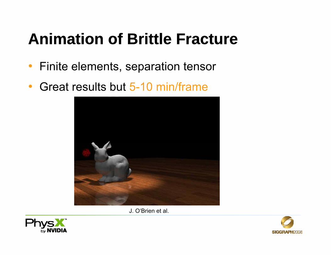
Animation of Brittle FractureAnimation of Brittle Fracture• Finite elements, separation tensor

• Great results but 5-10 min/frame

J. O‘Brien et al.

Real-Time Fracture of Stiff MaterialsReal-Time Fracture of Stiff Materials• Hybrid rigid body – static FEM

• Not quite as realistic but 30 fps

M.Müller et al. Eurographics CAS 2001

Deformables and WaterDeformables and Water

• Post doc with ETH computer graphics lab

2003 Video by D Charypar2004

FEM base deformables SPH fluids2003, Video by D.Charypar2004

NovodeX - AGEIANovodeX - AGEIA• 2003 NovodeX as ETH spin-off

• 2004 Acquisition by AGEIA

• 2007 Nils Thuerey AGEIA post docy p

Nils ThuereyNils Thuereyyy

• CV– 2007: PhD in computer science from University Erlangen

– 2007: Post doc with AGEIA

– 2008: Post doc with ETH

• Research interests– Lattice-Boltzmann based fluid simulation

– Real-time height field fluid simulationg

– Fluid Control

Offline PhysicsOffline Physicsyy• Applications

– Special effects in movies and commercials

• Typical setup– Millions of particles / triangles / tetrahedra / grid cells

– Expensive photorealistic rendering

– Impressive high quality results

– Seconds up to hours per frame

• Characteristics– Predictable re-run possible no interactionPredictable, re run possible, no interaction

Real Time PhysicsReal Time Physicsyy• Applications

I t ti t– Interactive systems

– Virtual surgery simulators („respectable“, „scientific“)

G ( t t bl b t t i 99%)– Games (not so respectable but true in 99%)

• Requirements– Fast, 40-60 fps of which physics only gets a small fraction

– Stable in any possible, non-predictable situation

• Challenge: – Approach offline results while meeting all requirements!Approach offline results while meeting all requirements!

From Offline to Real TimeFrom Offline to Real Time

• Resolution reduction– Blobby and coarse look

– Details disappear

• Use specialized real time techniques!– Physics low-res, appearance hi-res (shader effects)y , pp ( )

– Reduction of dimension from 3d to 2d (height field fluids, BEM)

– Level of detail (LOD)( )

– No equation solving, procedural animation for specific effects

Deformable ObjectsDeformable ObjectsDeformable ObjectsDeformable Objects

Examples of Deformable ObjectsExamples of Deformable Objectsp jp j

• 1d: Ropes hair• 1d: Ropes, hair

• 2d: Cloth, clothing

• 3d: Fat tires organs• 3d: Fat, tires, organs

DimensionalityDimensionalityyy

• Every real object is 3d

• Approximated object with lower dimentional models ifpossible

• Dimension reduction substantially saves simulation time

Mass Spring SystemsMass Spring Systemsass Sp g Syste sass Sp g Syste s

Mass Spring MeshesMass Spring Meshesp gp g

• Rope: chainRope: chain– Additional springs for bending

and torsional resistance needed

• Cloth: triangle mesh

S ft b d t t h d l h

– Additional springs for bendingrestistance needed

• Soft body: tetrahedral mesh

Mass Spring PhysicsMass Spring Physicsp g yp g y• Mass point: mass m, position x, velocity v

f -f

x m v

• Springs: xi xj

l0

⎥⎥⎦

⎤

⎢⎢⎣

⎡

−

−⋅−+−−

−

−=

ij

ijijdoijs

ij

ij klkxxxx

vvxxxxxx

f )()(

0

⎥⎦⎢⎣ ijij

• Scalars ks, kd, stretching, damping coefficients

Time IntegrationTime Integrationgg

• Newton:vxfv

==

&

& m/vx =

1 ),,,(1+ Δ+= ∑ tj

tj

ti

ti

ti

ti t vxvxfvv• Explicit Euler:

11 ++ Δ+=

∑t

it

it

i

jjjii

iii

t

m

vxx

• Assumes velocity and force constant within Δt

• Correct would be:

dttttttt

t∫Δ+

+=Δ+ )()()( vxx

• Correct would be:

t

Explicit Euler IssuesExplicit Euler Issuespp

• Accuracy– Better with higher order schemes e.g. Runge Kutta

– Not critical in real time environments

Δt2f/m• Stability Δt f/m– Overshooting

Big issue in– Big issue in real time systems!

Implicit IntegrationImplicit Integrationp gp g

• Use values of next time step on the right11111 ),,,(1 +++++ Δ+= ∑

j

tj

tj

ti

ti

i

ti

ti m

t vxvxfvv

• Intuitively

11 ++ Δ+= ti

ti

ti tvxx

• Intuitively– Don‘t extrapolate blindly

– Arrive at a physical configuration

Implicit Integration IssuesImplicit Integration Issuesp gp g

• Unconditionally stable (for any Δt)!

• Have to solve system of equations for velocities– n mass points, 3n unknownsp ,

– Non linear when the forces are non-linear in the positions as with springs

– Linearize forces at each time step (Newton-Raphson)

• Slow → Take large time stepsg p

• Temproal details disappear, numerical damping

Position Based DynamicsPosition Based Dynamicsos t o ased y a csos t o ased y a cs

Force Based UpdateForce Based Updatepp

penetration causes velocities changeforces change

• Reaction lag

penetration causes forces

velocities change positions

forces change velocities

• Reaction lag

• Small ks → squashy system

• Large ks → stiff system, overshooting

Position Based UpdatePosition Based Updatepp

penetration move objects so that

• Controlled position change

penetration detection only

move objects so that they do not penetrate update velocities!

• Controlled position change

• Only as much as needed → no overshooting

• Velocity update needed to get 2nd order system!

Position Based IntegrationPosition Based IntegrationggInit all xi

0, vi0

LLooppi = xi

t + Δt·vit // prediction

x t+1 = modify p // position correctionxi = modify pi // position correctionui = [xi

t+1 – xit] /Δt // velocity update

vit+1 = modify ui // velocity correction

• Explicit Verlet related

i y i yEnd loop

• Explicit, Verlet related

• If correction done by a solver → semi implicit

Position CorrectionPosition Correction• Move vertices out of other objects

• Move vertices such that constraints are satisfied

• Example: Particle on circlep

prediction

correctionnew velocity

Velocity CorrectionVelocity Correctionyy• External forces: vt = ut + Δt·g/m

• Internal damping

• Friction

• Restitutioncorrected

l it

collision correction

prediction

restitutionfriction

velocity

collision correction

Internal Distance ConstraintInternal Distance Constraint

( ) 21021

11

xxxxx −−−−=Δ lwΔx2 ( )

21021

211 xx −+ ww

( ) 21021

22

xxxxx −−−+=Δ lw

m1

m2l0Δx1

ii mw /1=

( )21

02121

2 xx −+ wwm1

• Conservation of momentum

• Stiffness: scale corrections by k ∈ [0..1]

• Easy to tune but effect dependent on time step!

General Internal ConstraintGeneral Internal Constraint• Define constraint via scalar function:

02121 ),( lCstretch −−= xxxx

[ ] 01413124321 6)()()(),,,( vCvolume −−⋅−×−= xxxxxxxxxx

C=0 ∇C∇C

Rigid body modes

General Position CorrectionGeneral Position Correction

• Correction along gradient),...,( 1 nii Cws

ixxx x∇−=Δ

• Correction along gradient

C )(

• Scalar s tells us how far to go

∑ ∇=

j nj

n

CwCs 2

1

1

),...,(),...,(

xxxx

x

Shape Matching IdeaShape Matching Ideap gp g

• Optimally matchd f d ithundeformed with

deformed shape

O l ll t l ti pi

Δxi

• Only allow translationand rotation

Gl b l ti

pi

• Global correction, no propagation needed

• No mesh needed!• No mesh needed!

Shape MatchingShape Matchingp gp g• Let xi be the undeformed vertex positions

• The optimal translation is

cmcm xpt −= ∑∑∑∑ ==i

iii

icmi

iii

icm mmmm / and / xxppwhere

• The optimal linear transformation is 11

))(())((−

⎟⎠

⎞⎜⎝

⎛−−⎟

⎠

⎞⎜⎝

⎛−−= ∑∑ T

cmicmii

iT

cmicmii

i mm xxxxxxppA

• The optimal rotation R is the rotational part of A(use polar decomposition)

2d Shape Matching Demo2d Shape Matching Demop gp g

Working with Points and EdgesWorking with Points and Edgesg gg g• No notion of volume or area

– Spring stiffness (N/m) not related to 3d stiffness (N/m2)

• Volumetric behavior dependent on– Tesselation of volume

– Hand tune spring stiffnesses

• Often OK in real time environments– Evenly tesselated physics meshesEvenly tesselated physics meshes

– Fixed time step

Co-Rotated Finite ElementsCo-Rotated Finite ElementsCo otated te e e tsCo otated te e e ts

Continuum Mechanics on one SlideContinuum Mechanics on one Slide

• Body as continuous set of points p(x)Body as continuous set of points

• Deformation continuous function p(x)

Elasticit theor ields f ( ) from ( )

p(x)

• Elasticity theory yields felast(x) from p(x)

• PDE of motion (Newton): x

),(),(),( ttt extelasttt xfxfxp +=ρ

• Solve for p(x t)• Solve for p(x,t)

• Analytical solution only for very simple problems

Finite Element Method on one SlideFinite Element Method on one Slide• Represent body by set of finite elements (tetrahedra)

• Represent continuous p(x) by vectors pi on verticesx3 p3 p1p1

x0

x1x2

p2

p0

• pi induce simple continuous p(x) within each element

• Continuous elasticity theory yields forces at vertices

Hyper SpringHyper Springyp p gyp p g• Vertex forces depend on displacements of all 4 vertices

)(][ ffff

• Tetrahedron acts like a hyper spring

),,,,,,,(],,,[ 321032103210 xxxxppppffff tetraF=

• Tetrahedron acts like a hyper spring

• Compare to: [f0, f1] = Fspring(p0,p1,l0)

• Given Ftetra () -blackbox, simulate as mass spring system

• Ftetra () is non linear, expensive

LinearizationLinearization• Linearization Ftetra () of yields

000

⎥⎥⎤

⎢⎢⎡

−−

⎥⎥⎤

⎢⎢⎡

xpxp

ff

1212

33

22

11

3

2

1 , ×∈

⎥⎥⎥

⎦⎢⎢⎢

⎣ −−

=

⎥⎥⎥

⎦⎢⎢⎢

⎣

RK

xpxpxp

K

fff

333 ⎦⎣⎦⎣ p

• K depends on x0, x1, x2, x3 and can be pre-computed(see class notes for how to compute)

• Much faster to evaluate

Linearization ArtifactLinearization Artifact

• Linearization only valid close to fthe point of linearization

f

x p

linearized non-linear

Corotational FormulationCorotational Formulation

• Only rotations problematic, translations OK

• Extract rotation: RK(RTp-x)

p-xRf

RT

K(RTp-x)RTp-xp

Rotational PartRotational Part

• Modified force computation

⎟⎟⎟⎞

⎜⎜⎜⎛

⎥⎥⎤

⎢⎢⎡

⎥⎥⎤

⎢⎢⎡

⎥⎥⎤

⎢⎢⎡

⎥⎥⎤

⎢⎢⎡

1

0

1

0

1

0

xx

pRpR

K00R0000R

ff

T

T

⎟⎟⎟

⎠⎜⎜⎜

⎝⎥⎥⎥

⎦⎢⎢⎢

⎣

−

⎥⎥⎥⎥

⎦⎢⎢⎢⎢

⎣⎥⎥⎥

⎦⎢⎢⎢

⎣

=

⎥⎥⎥

⎦⎢⎢⎢

⎣ 3

2

3

2

1

3

2

xx

pRpR

K

R0000R00

ff

T

T

• Transformation matrix1

030201030201 ],,][,,[ −−−−−−−= xxxxxxppppppA 030201030201 ],,][,,[ pppppp

• Rotation via polar decomposition of A

AdvantagesAdvantagesgg

• Matrix K can still be precomputed

• Artifacts removed

• Faster force computation in explicit• Faster force computation in explicit formulation

• Implicit time integration yields linear system→ no Newton-Raphson solver neededp

FEM DemoFEM Demo

ConclusionsConclusions

• Trade-off speed, accuracy, stability

• Choose method accordingly

• Stability most important in real time systems• Stability most important in real time systems– Non predictable situations

– No time step adaptions

– No roll backs

• Remaining choice: accuracy vs. speed

Cloth in GamesCloth in Games

Mesh GenerationMesh Generation

• Input – Graphical triangle surface mesh

– Extreme case: Triangle soupg p

• Output– Input independent tesselation

– User specify resolution (LOD)

– Equally sized elements (stability, spatial hashing)

Surface CreationSurface Creation

• Input triangle mesh

• Each triangle adds densityto a regular gridto a egu a g d

• Extract iso surface using marching cubesg

• Optional: Keep largest connected mesh onlyy

• Quadric simplification

Tetrahedra CreationTetrahedra Creation• Delaunay

Tetrahedralization onTetrahedralization on vertices of surface mesh

• Triangles of surface meshTriangles of surface meshare used for clippingtetrahedra (if necessary)

• Graphical mesh is movedalong with tetra meshusing barycentric coords